Article

Pattern of Turbidity Change in the Middle Reaches of the Yarlung Zangbo River, Southern Tibetan Plateau, from 2007 to 2017

1
Department of Geography, The University of Tennessee, Knoxville, TN 37996, USA
2
State Key Laboratory of Urban and Regional Ecology, Research Center for Eco-Environmental Sciences, Chinese Academy of Sciences, Beijing 100085, China
3
Department of Electrical Engineering and Computer Science, The University of Tennessee, Knoxville, TN 37996, USA
4
Key Laboratory of Digital Earth Science, Aerospace Information Research Institute, Chinese Academy of Sciences, Beijing 100094, China
*
Author to whom correspondence should be addressed.
Submission received: 13 November 2020 / Revised: 30 December 2020 / Accepted: 5 January 2021 / Published: 7 January 2021

Abstract

:
Turbidity is an important indicator of riverine conditions, especially in a fragile environment such as the Tibetan Plateau. Remote sensing, with the advantages of large-scale observations, has been widely applied to monitor turbidity change in lakes and rivers; however, few studies have focused on turbidity change of rivers on the Tibetan Plateau. We investigated the pattern of turbidity change in the middle reaches of the Yarlung Zangbo River, southern Tibetan Plateau, based on multispectral satellite imagery and in situ measurements. We developed empirical models from in situ measured water leaving reflectance and turbidity, and applied the best performed s-curve models on satellite imagery from Sentinel-2, Landsat 8, and Landsat 5 to derive turbidity change in 2007–2017. Our results revealed an overall decreasing spatial trend from the upper to lower streams. Seasonal variations were observed with high turbidity from July to September and low turbidity from October to May. Annual turbidity showed a temporally slightly declining trend from 2007 to 2017. The pattern of turbidity change is affected by the confluence of tributaries and the changes in precipitation and vegetation along the river. These findings provide important insights into the responses of riverine turbidity to climate and environmental changes on the Tibetan Plateau.

Graphical Abstract

1. Introduction

Climate change has had significant impacts on the high-altitude and fragile environment of the Tibetan Plateau in recent decades [1]. Permafrost degradation [2], glacier melting, and desertification [3] have been accelerated, affecting the water environment of the plateau [4]. As one of the main water resources, rivers are facing severe challenges on the Tibetan Plateau due to climate and environmental changes, as well as the increasing demand of qualified water for human lives and socioeconomic development [5].
Turbidity is an important indicator of water quality and hydrological conditions of rivers. As a measure of water transparency, turbidity is associated with the concentration of total suspended sediments and other impurities in the water [6]. It is commonly monitored by field measurement and hydrological station observations, which are usually time-consuming and only limited to discrete sites. With the advantage of broad coverage and low costs, remote sensing provides an alternative way to monitor turbidity at various spatial and temporal scales [7]. The integration of in situ measurements and remote sensing data allows for a coherent quantification of turbidity changes, especially in remote alpine regions.
Remote sensing imagery has been used to derive turbidity based on a variety of empirical, semiempirical, and analytical models [8,9]. The common strategy of these models is to establish the relationships between turbidity and image reflectance based on the calibration of in situ measurement of water samples [10]. Simple linear models have been found to be effective and robust for turbidity estimation [11]. However, when suspended sediments increase to high concentrations (>50 mg/L), the relationship between turbidity and image reflectance becomes nonlinear and the sensitive wavelength shifted from visible (VIS) bands to longer wavelength near-infrared bands (NIR) [12,13]. Exponential relationships have been used to derive the turbidity of water with high concentrations (>50 mg/L) of suspended sediments [14,15]. Studies suggested that the red band reflectance has the best performance in terms of retrieving turbidity from multispectral satellite imagery, including Medium Resolution Imaging Spectrometer (MERIS), Thematic Mapper (TM), Enhanced Thematic Mapper Plus (ETM+), Moderate Resolution Imaging Spectroradiometer (MODIS), High-resolution Visible and medium InfraRed (HRVIR), and Advanced Visible and Near Infrared Radiometer (AVNIR) [16,17,18]. Laboratory experiments also demonstrated that suspended particulate matter (SPM) has the highest sensitivity to the reflectance of 550–650 nm [19,20]. Based on established models, satellite imagery has been applied to monitor seasonal and long-term turbidity changes [21,22]. Turbidity has been found as a robust indicator for several water quality components, including total suspended sediments, Chlorophyll-a (Chi-a), Total Phosphate (TP), and Total Nitrogen (TN) [23]. The distribution pattern of turbidity is affected by rainfall, runoff, and spring tides [22]. These studies, however, are mostly site-specific and it is hard to extend the relationships established from these studies to different water bodies.
The Yarlung Zangbo River (YZR) is the largest river on the Tibetan Plateau [24]. It provides a freshwater supply to Tibetan people [25] and acts as an important corridor to transfer moisture from the Indian Ocean to the Tibetan Plateau [26]. As the upper reaches of an international river (Brahmaputra River) flowing from China to India and Bangladesh, the YZR plays an essential role in water consumption and environment conservation in this region [27,28]. The YZR basin is the economic and cultural center of the Tibetan Autonomous Region, China, occupied by over half of the Tibetan population [29]. However, the water environment in the YZR is fragile and vulnerable to climate change and human interventions [27,30]. It is important to monitor turbidity change of the YZR because it is critical to the socioeconomic development and ecological stability in this region. Water quality of the YZR was first reported in 1982, focusing on major ions [31]. Recent studies investigated the distributions and concentrations of mercury (Hg) [26], total phosphorus (TP) [27], metal elements [29], major chemical compositions [32], and suspended sediments [6,30,33]. However, most these studies only relied on the scattered observations from gauging stations. The temporal and large-scale spatial characteristics of turbidity change are still poorly known due to the difficulties to conduct field survey on the remote, high altitude, and harsh environment of the YZR [4]. Given its uniqueness, the empirical remote sensing models developed from other lakes and rivers are likely not suitable for turbidity monitoring of the YZR. There is an urgent need to develop suitable remote sensing-based turbidity models to support environment conservation and resource management in this region.
In the work reported here, we investigated the spatial and temporal pattern of turbidity change in the YZR based on Landsat and Sentinel-2 imagery and examined the impacts of climate and environmental factors on this pattern. Specifically, we first investigated the relationships between turbidity and spectral signatures of in situ collected water samples to develop empirical models for turbidity monitoring. Then, we derived the spatial and temporal patterns of turbidity changes in the middle reaches of the YZR from 2007 to 2017 based on Sentinel-2, Landsat 5, and Landsat 8 imagery. Finally, we explored the effects of tributaries, precipitations, and vegetations on turbidity change in this area. This work provides important insights into the responses of riverine turbidity to climate and environmental changes on the Tibetan Plateau.

2. Materials and Methods
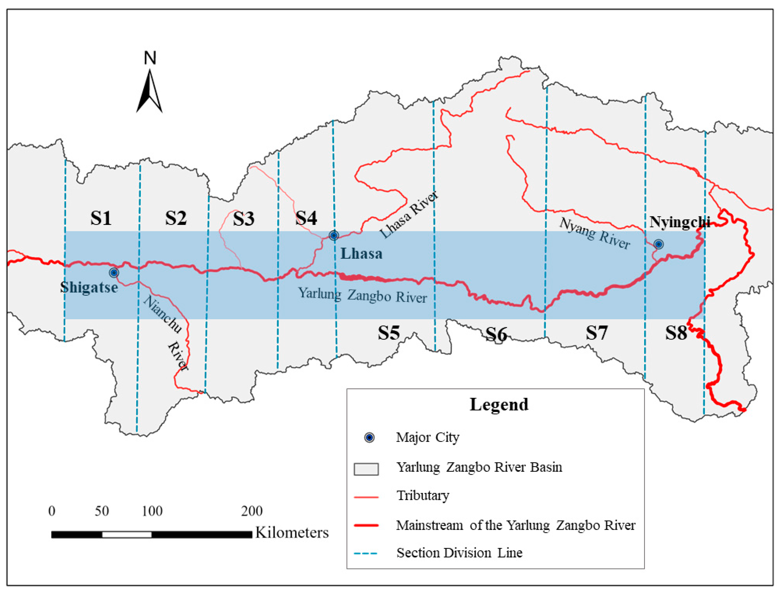
2.1. Study Area

The YZR is one of the highest rivers in the world, flowing from west to east along the valleys of the southern Tibetan Plateau [6]. It originates from the Gyima Yangzo Glacier on the southeast of Mount Kailash, northern Himalayas, with a length of about 2057 km and a drainage area of approximately 240,480 km2 [34]. The YZR is the largest river on the Tibetan Plateau with an average elevation of ~4600 m (ranging from 147 to over 7000 m) above sea level [35]. As elevation descends from west to east, vegetation gradually changes from cold desert, to arid steppe, deciduous scrub, and ultimately to conifer and rhododendron forest [36]. Fed by both snowfall and rainfall, the YZR have perennial flow throughout the year [29]. The river transports a large amount of sediments from the Himalayas and the Tibetan Plateau to the Indian Ocean. It is also a natural corridor for the South Asian Monsoon, transferring airmass and moisture from the Indian Ocean to the Tibetan Plateau [32].
Our study focuses on the middle reaches of the YZR from Lizicun in Zhongba County, Shigatse, to Pei in Mainling County, Nyingchi (Figure 1). This area is characterized by broad intermontane valley basins. The climate is a temperate plateau climate with relatively abundant moisture from the monsoon [37]. Precipitation mainly occurs from June to September during the wet season with an annual average of 300–600 mm [34,38,39]. The type of precipitation is mainly rainfall from May to October and snowfall for the remaining months [40]. The annual mean temperature is −0.44 °C with an annual maximum temperature of 6.84 °C in summer and minimum temperature of −6.92 °C in winter. With the continuous drop in elevation, it becomes warmer and wetter from upper to lower streams in this YZR section [35]. Three main tributaries, Nianchu River, Lhasa River, and Nyang River, flow into the middle reaches of YZR. Three cities of Shigatse, Lhasa, and Nyingchi are located close to the confluences of these three tributaries, respectively. Accounting for only 5% of the total area and 10% of the cultivated area, the YZR basin is the principal agricultural region of the Tibetan Automatic Region, producing more than half of the total agricultural production and feeding more than half (about 1.5 million) of the residents [41]. It is challenging to maintain a harmonious human–environment relationship in this area due to the fragile environment and continuously increased human demands.

2.2. Datasets

2.2.1. In Situ Measurement

To develop accurate turbidity models, we collected water samples and measured water-leaving reflectance at 40 sites along the middle reaches of YZR in September 2016 (Figure 1). Although sampling was limited by inaccessible streams with high flow velocity or steep riverbanks, we tried to sample representative water environments, including streams before and after confluences of major tributaries, and streams of different widths. The sampling sites were distributed in four regions: mainstream near the confluence of Lhasa River (included the widest stream section of the YZR), mainstream near the confluence of Nyang River, and the two tributaries of Lhasa River and Nyang River (Figure 1b,c).
Water samples were collected away from the riverbanks and stored properly in polypropylene bottles. Water sample analysis was conducted in the State Environment Protection Key Laboratory of Ecological Effects and Risk Assessment of Chemicals, Chinese Research Academy of Environmental Sciences [42]. Water turbidity was measured by spectrophotometry (UNICO WFZ UV-2800HA) with Nephelometric Turbidity Units (NTUs). The measurement procedure was detailed in article [43].
Water-leaving reflectance was measured by the Analytical Spectral Devices (ASDs) FieldSpec® 3 field portable spectrometer (Malvern Panalytical, Malvern, UK). This spectrometer has a wavelength ranging from 350 to 2500 nm with a sampling interval of 1.4 nm for the range of 350–1000 nm and 2 nm for the range of 1001–2500 nm [44]. The ASD spectroradiometer was calibrated for each sampling site to adjust the light conditions before taking the measurement. We measured the spectrums from the reference board and river water surface for each sampling site. The measurement was taken with a vertical downward view at a 30 cm height above the surface under clear-sky conditions. The reference board was placed on a flat surface near each measured site. Ten spectral measurements were taken consecutively and averaged to minimize the random errors from the surrounding environment. Water bodies are weak radiators with lower reflectances than other land cover types. The mixed spectrums from turbid water, river bottom, and adjacent land surfaces were complicated due to varied stream width, depth, and velocity [45,46]. To reduce the effects of the reflection from the river bottom and surrounding objects, in addition to the use of reference white boards for calibration, we measured water-leaving radiance as far away from the riverbanks as possible. We also avoided the locations with visible river bottoms and mitigated the effects of the surrounding environments in the field survey.
Water-leaving reflectance was calculated for each sampling site based on the paired digital numbers recorded by ASD for the reference white board and water surface, respectively. The equation for the calculation is [47]:
Ref water = DN water DN reference × Ref reference
where Ref water is the water-leaving reflectance; DN water and DN reference are the ASD-recorded digital numbers from the water surface and reference board, respectively; Ref reference is the reflectance from the reference board (0.994 in this study).
We plotted the spectral curve to examine the derived water-leaving reflectance for each sample site. The spectral curves of four sample sites have abnormal fluctuations due to the unstable power supply for the ASD [44]. We removed these four measurements and used the water-leaving reflectance measurements from the remaining 36 sample sites and their corresponding water turbidities for further analysis. The reflections become noisy at >950 nm due to the strong absorption by water. We therefore only used the visible to near-infrared spectrum (350–900 nm) for the analysis.
To make the reflectance derived from the in situ measurements comparable to the reflectance recorded on satellite imagery, we integrated the equivalent spectral channels of each sensor from the field-measured continuous water-leaving spectral curves based on Equation (2) [48]:
ρ ( λ ) R S = λ min λ max ρ ( λ i ) f ( λ i ) d λ λ min λ max f ( λ i ) d λ
where λ is the central wavelength of a satellite sensor, [ λ min , λ max ] is the range of the spectral channel, ρ ( λ i ) is the measured water-leaving reflectance at λ i , f ( λ i ) is the spectral response function of the sensor, and ρ ( λ ) R S is the derived remote sensing reflectance at the band λ .

2.2.2. Remote Sensing Imagery

Multispectral images from Landsat and Sentinel programs were used to monitor turbidity changes in the YZR. Landsat has collected high-quality and global coverage imagery since the 1970s. It provides a useful collection of satellite imagery for long-term monitoring of earth surface changes, including inland water bodies [21,22,23]. Landsat 5 was launched in 1984 and decommissioned in 2013. It carried two sensors—Multispectral Scanner System (MSS) and Thematic Mapper (TM). Landsat 8 has been operating since 2013 with two sensors of the Operational Land Imager (OLI) and the Thermal Infrared Sensor (TIRS). Sentinel-2 was launched in 2015 with the Multispectral Instrument (MSI) sensor on board. Compared to Landsat, it has the advantages of higher revisit time, finer spatial resolution, and more spectral bands. Similar spectral bands between Sentinel-2 and Landsat images enable data combination for long-term monitoring studies. The Sentinel-2 MSI also includes unique bands with narrow band widths at the red edge and near-infrared wavelengths to refine water turbidity monitoring. Table 1 lists main technical specifications of the bands for the Landsat and Sentinel-2 images used in this study.
We manually selected 406 scenes of cloud-free and clear images of the study area, including 227 Landsat 5 TM images in 2007–2011, 119 Landsat 8 OLI images in 2013–2017, and 60 Sentinel-2 MSI images in 2016–2017. Landsat images were downloaded from Earth Explorer [49] and Sentinel-2 images were downloaded from Copernicus Open Access Hub [50]. No clear images were available in 2012, making it a gap year. Table 2 lists the number of images used in this study.
The downloaded images were Level-1 products, organized as tiled and radiometrically and geometrically corrected Top-Of-Atmosphere (TOA) digital numbers. Sentinel-2 images were processed by the Sentinel-2 toolbox on the Sentinel Application Platform (SNAP), which is developed by European Space Agency (ESA) for visualizing, analyzing, and processing the Sentinel-2 datasets [51]. Sen2Cor is the atmospheric correction tool provided in SNAP [52]. We first conducted the atmospheric correction of the Sentinel-2 images by Sen2Cor version 2.8 and resampled all bands to the same resolution of 10 m. Atmospheric correction of Landsat images were conducted by Quick Atmospheric Correction (QUAC) model on ENVI image analysis software (the leading software for image processing and analysis solutions), which works well for Landsat imagery in inland water studies [53]. All images were then converted to Bottom-Of-Atmosphere (BOA) reflectance and water pixels were extracted based on the Modified Normalized Difference Water Index (MNDWI) from all corrected images [54,55]. The thresholds for water pixel extraction were determined by visual interpretation.
Note that atmospheric radiance and radiance scattered after interacting with the surrounding land surfaces account for a majority of signals received by satellite sensors at water pixels. This is known as an adjacency effect, one of the major factors affecting the quality of remotely sensed imagery [32]. We therefore used the internal parameters and specific designed algorithms of the satellite products to correct the images before developing turbidity models. We also applied a 3*3 filter to remove the potential noises caused by surrounding environments.

2.2.3. Auxiliary Data

We downloaded precipitation and Normalized Difference Vegetation Index (NDVI) data to investigate their impacts on turbidity change. The monthly precipitation data were downloaded from National Tibetan Plateau Data Center [56]. This dataset is formatted as NetCDF with a spatial resolution of 1 km from Jan 1901 to Dec 2017. We converted and extracted the monthly precipitation in our study area using ArcGIS Pro 2.4. The NDVI data were archived as annual NDVI products on Google Earth, composited using Landsat 5 and 8 images with a spatial resolution of 30 m [57,58]. We extracted the mean NDVI data for each stream section using Google Earth Engine Code Editor.

2.3. Turbidity Models

Turbidity models were developed based on the correlations between in situ measured turbidity and water-leaving reflectance. We evenly selected 12 out of the 36 paired in situ measurements of water turbidity and water-leaving reflectance based on the turbidity levels for model validation. The remaining 24 paired measurements were used for model development. Turbidity models were developed separately for different sensors (Landsat 5 TM, Landsat 8 OLI, and Sentinel-2 MSI) to avoid the uncertainties caused by their band differences.
We first evaluated the sensitivity of each sensor band before developing the turbidity models. Pearson’s correlation coefficient was calculated between integrated reflectance of each band and measured turbidity. We also used band ratios in the correlation analysis to reduce the effects of bidirectional reflectance variations and environmental interference [12]. The highly correlated band reflectance or band ratios were then selected to develop the regression models for turbidity using different satellite images. We compared eight regression models listed in Table 3 to determine the most suitable model in the YZR.
We used the coefficient of determination (R2), root-mean-square deviation (RMS), relative error (RE), and mean relative error (MRE) to evaluate the performance of each model. R2 measured how well the regression model described the observed data [59]. RMS measured the averaged difference between the predicted and observed turbidity values, while RE and MRE measured the relative difference between the predicted and observed turbidity values [60]. These parameters were calculated by Equations (3)–(6), respectively,
R 2 = 1 i = 1 n ( x obs , i x mod , i ) 2 i = 1 n ( x obs , i x ¯ obs ) 2
RMS = i = 1 n ( x mod , i x obs , i ) 2 n
RE = | x mod , i x obs , i x obs , i | × 100 %
MRE = 1 n | x mod , i x obs , i x obs , i | × 100 %
where n is the number of samples, x obs , i is the observed turbidity of i-th sample, x ¯ obs is the observed mean turbidity, and x mod , i is the predicted turbidity of i-th sample. We preferred to adopt the models with high R2 values and low RMSs and MREs for further analysis. All statistical analyses were conducted by SPSS 23 [61] and R 3.5.2 [62].

2.4. Turbidity Pattern Analysis

We divided the whole stream into 8 sections to examine the pattern of turbidity changes (Figure 2). These sections include two upper stream sections (S1, S2), four middle stream sections (S3, S4, S5, S6), and two lower stream sections (S7, S8). S5 is the widest section of the river. For each satellite image, the mean turbidity was calculated by averaging the turbidity values of all water pixels in each section. The two tributaries, Lhasa River and Nyang River, flow into the YZR at S3–S4 and S7–S8, respectively. The turbidity values of the two tributaries were also derived using the same models and averaged for each tributary to investigate the effect of tributary confluence on spatial turbidity patterns. We did not include the Nianchu River in the analysis due to the lack of in situ measurements. We collected in situ measurements from both Lhasa and Nyang rivers and these measurements were also used for model development and validation (Figure 1).
A previous study showed that the influences of vegetation on water quality are prominent within 200 me of the river channel, while the impacts are sharply decreased where the distance is >300 m away from the river [63]. We therefore created a buffer zone of 200 m on both sides to the YZR to extract the mean NDVI for each river section. Monthly mean precipitation was extracted along each river section. We used Pearson correlation coefficients to quantify the impacts of tributary confluence, precipitation, and NDVI on turbidity changes.

3. Results

3.1. Turbidity and Spectral Signatures of the YZR

Figure 3 illustrates the turbidity values of the water samples collected in different regions of the YZR. The results indicate that the turbidity levels of the mainstream are higher than those of the tributaries. Along the mainstreams, the turbidity levels in the upper section near the Lhasa River are higher than those in the lower section near the Nyang River. The turbidity levels of Lhasa River are also higher than those in the Nyang River.
In situ collected water-leaving reflectance varies at different turbidity levels. Figure 4 illustrates the spectral curves of different turbidity values measured in the field. Most of the spectral curves are bimodal from 350 to 950 nm. The water-leaving reflectances are lower than 20%, indicating the sampled water absorbs and transmits most radiance reaching river surface and reflects <20% back to the atmosphere. The water reflects more visible light than infrared radiation and the highest reflectance occurs from 580 to 720 nm. The other relatively weak and narrow reflection peak occurs near 810 nm. As turbidity increases, the overall reflectance elevates, and the main reflectance peak becomes wider. Distinct differences caused by turbidity occur around 550–700 nm and 800–850 nm, making green, red, and near-infrared the suitable bands to quantify turbidity. These bands have also been implemented to retrieve turbidity information in other studies [12,21,64].

3.2. Turbidity Models

We examined the correlations between turbidity of water samples and spectral indices of an equivalent sensor’s reflectance derived from measured water-leaving reflectance. Spectral indices include single band reflectance, band ratios, and normalized difference indices similar to the format of NDVI. As listed in Table 4, the correlation coefficients between the spectral indices and measured turbidity range from −0.023 (of green band) to 0.761 (of red/green band ratio). The correlations between turbidity and single band reflectance are not statistically significant. In contrast, most correlations for band ratios are statistically significant. Normalized difference indices also provide significant correlations but the coefficients are lower than those of band ratios. The red/green band ratio has the highest correlation coefficient with turbidity.
Table 5 lists the correlations between turbidity and spectral indices of the narrow bands of Sentinel-2 MSI images. The ratios of the blue, green, and red bands perform better than the single band. Correlation coefficients of red edge/green band ratios and turbidity are relatively higher than other spectral indices. Nonetheless, the correlation coefficient between the red/green band ratio and turbidity is still the highest (Table 4 and Table 5). Therefore, the red/green band ratio was selected to develop the turbidity models.
We explored various regression models to predict turbidity using the red/green band ratio. Table 6 lists the performances of the eight regression models for different sensors based on 24 model development samples. We noticed that the MREs are not as good as expected. Taking the models for Sentinel-2 MSI imagery as examples, the R2 values range from 0.563 to 0.766, indicating these regression models can explain 56.3–76.6% of the variances between turbidity and the red/green band ratio. Although these models could explain more than half of the observed variances, the MRE values range from 0.488 to 1.309, indicating the average errors predicted by these models vary from 48.8% to 130.9% of the observed turbidity values. We further examined the relative errors of each sample to investigate the model performances at different turbidity levels.
Figure 5 illustrates the relative errors of each sample for different models. It seems that high relative error occurs when turbidity is low, especially at 5 NTU. The highest relative error at 5 NTU is caused by negative predictions from the linear, logarithmic, and inverse model, indicating these models are not robust for predicting turbidity at a large range. Another two peaks of relative errors occur at 15 and 25 NTU, respectively. The relative error decreases as turbidity increases, while no obvious trend exists when turbidity is >30 NTU. We compared the MRE values for all model development samples and samples of turbidity >30 NTU (Table 7). The MRE value decreases from 1.3 to 0.48 for all samples and to 0.2–0.3 for the samples with turbidity of >30 NTU. The linear, logarithmic, inverse, quadratic, and cubic models provide higher MRE values for all samples and relatively lower MREs for higher turbidity samples, indicating that these models may be more reliable for samples with turbidities of >30 NTU. Other models, including power, s-curve, and exponential models, do not show large deviations of MRE for different turbidity levels.
We prefer to adopt the turbidity model with a high R2, low RMS, and low MRE for different turbidity levels since turbidity varies at a wide range in the YZR. The exponential, power, and s-curve models show relatively higher R2 (>0.75) and lower overall MRE (<0.5) values and provide small MRE deviations at different turbidity levels. The s-curve model exhibits the lowest RMS and MRE values for higher turbidity samples of >30 NTU (Table 6 and Table 7). Therefore, we selected the s-curve model for turbidity monitoring in the YZR based on the red/green band ratio.
We also validated the fitted s-curve models based on the 12 validation samples. The RMS values of these validation samples are lower than those of the model development samples and the MRE values of the samples with turbidities of > 30 NTU are lower than 0.2, suggesting that the average estimation accuracy is more than 80% for these samples. These results validated the good performance of the fitted s-curve models, especially for samples with turbidities of >30 NTU (Table 8). We also draw the scatter plots between the measured and estimated turbidity values to check the performance of the s-curve models (Figure 6). Most model-predicted and field-measured turbidity values are scattered along the y = x line, indicating relatively good performances. Exceptions occur when the measured turbidity values are around 10 and 150 NTU; at these values the models tend to slightly overestimate the low turbidity values and underestimate the high turbidity values. Given the good performances for both modelling and validation samples, we used the three fitted s-curve models for Landsat 5 TM, Landsat 8 OLI, and Sentinel-2 MSI images to estimate the turbidity in the YZR, respectively.

3.3. Turbidity Patterns

We calculated the red/green band ratio of the preprocessed 406 satellite images from Landsat 5 TM, Landsat 8 OLI, and Sentinel-2 MSI, and derived turbidity values based on the s-curve models described in Section 3.2. The turbidity values were then averaged for each stream section to evaluate the spatial and temporal changes. The turbidity values derived from images acquired in the same month in a year were also averaged to derive the monthly turbidity value. We analyzed the temporal turbidity variations at all eight sections, but just illustrated the results at S2, S4, S5, and S7 in figures due to the similar turbidity patterns of some adjacent sections. The upper section was represented by S2. The middle section was represented by S4. The widest section was S5. The lower section was represented by S7.

3.3.1. Spatial Pattern of Turbidity Change in the YZR

The average turbidity shows an overall downstream decreasing trend from upper to lower stream sections in the YZR (Figure 7). Turbidity is relatively high at S1 close to Shigatse where the Nianchu River joins the YZR. It decreases before the confluence of the Lhasa River (S3) and increases after the tributary joins (S4). Relatively high turbidity occurs at the upper stream of S1 and the widest section of S5. Turbidity decreased again from S5 to S7 and the confluence of another tributary, Nyang River, caused a slight increase in turbidity from S7 to S8.

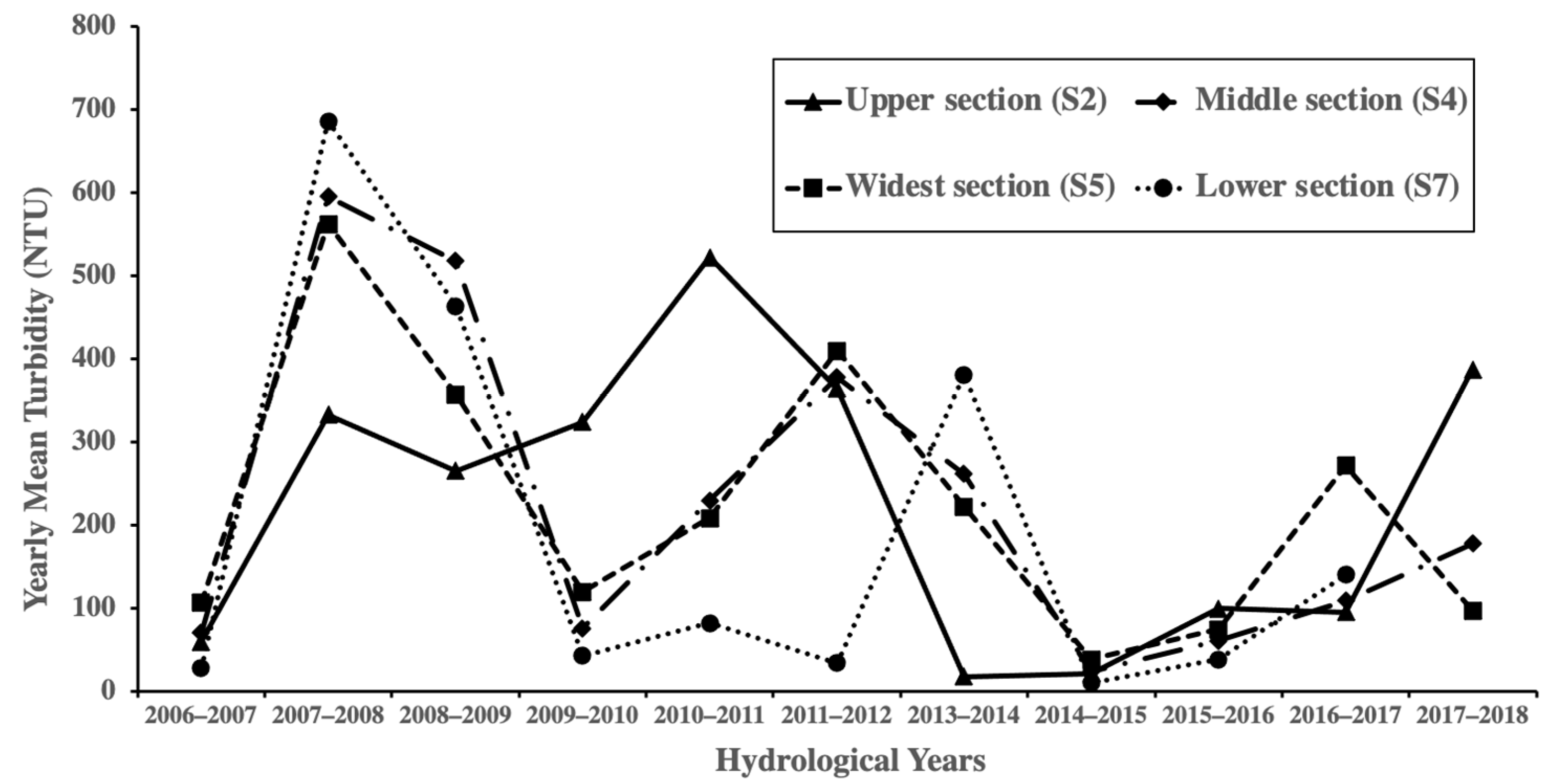
3.3.2. Temporal Pattern of Turbidity Change in the YZR

Our results show both seasonal and annual changes in turbidity in the middle reaches of the YZR from 2007 to 2017. In terms of seasonal change, turbidity is much higher from June to September than the other months (Figure 8). Turbidity stays relatively stable from January to May, then starts to increase from June to September. It reaches the peak in July or August and decreases from October to December. It then remains a relatively low level similar to the months before June. This seasonal pattern was observed in all sections in the middle reaches of the YZR.
Considering the seasonal variations in turbidity, we evaluated the annual turbidity changes based on the hydrological year that starts from the first day of the dry season (1 October) and ends at the last day of the next wet season (30 September). A slightly declining trend in turbidity was observed from 2007 to 2017 (Figure 9). The annual turbidity changes presented similar variations for the middle, widest, and lower sections where turbidity reached the first peak in the hydrological years of 2007–2009 and another peak in 2011–2014. The turbidity values at the upper section were relatively higher in 2010–2011 and 2017–2018 hydrological years.

3.4. Turbidity Change with Environmental Factors

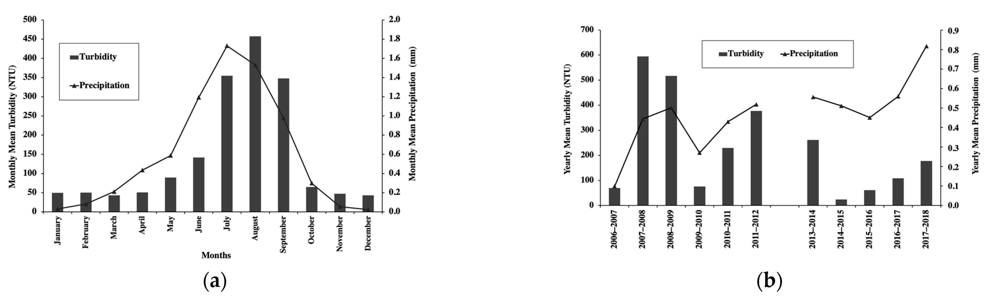
3.4.1. Turbidity Change with Precipitation

Precipitation is an important factor affecting river turbidity. More precipitation increase the amount and velocity of the runoff that erodes and transports more sediments into the river, increasing the turbidity [65]. The impact of precipitation is especially apparent in the dry and less-vegetated areas [66]. We compared the temporal and spatial change of turbidity with precipitations in Figure 10 and Figure 11. Seasonal and interannual changes of turbidity demonstrate similar patterns to those of precipitation. High turbidity and precipitation both occur during the summer from June to September (Figure 10a). The “wetter” hydrological year with high precipitation (2007–2008, 2008–2009, 2011–2012, 2013–2014) experienced high turbidity levels while the “drier” hydrological year with low precipitation (2006–2007, 2009–2010, 2015–2016) experienced low turbidity levels (Figure 10b).
Spatially, we also observed different temporal patterns between turbidity and precipitation at different sections (Figure 11). In the upper to middle sections from S1 to S5, turbidity shows the same trend as precipitation, slightly decreasing from S1 to S3 then increasing to S5. In the lower sections from S6 to S7, turbidity decrease regardless of the increasing precipitation. Compared with the upper and middle sections, precipitation is much higher in lower sections, although turbidity values are relatively lower.

3.4.2. Turbidity Changes with Normalized Difference Vegetation Index (NDVI)

Vegetation mitigates turbidity in rivers by preventing soil erosion and absorbing pollutants [63]. As a proxy of vegetation cover, the mean annual NDVI within a 200 m buffer zone along each section was extracted and examined with turbidity change. Spatially, NDVI is the lowest in the middle section and the highest in the lower section (Figure 12). Temporally, the lower section experienced relatively large NDVI variations with a decreasing trend from 2007 to 2017, while the NDVIs of other sections slightly increased with minor fluctuations from 2008 to 2017 (Figure 12). However, turbidity change does not agree well with the NDVI change. In the upper, middle, and widest sections, several high turbidity values occurred during low NDVI years (2008, 2011, 2013). In contrast, high turbidity values occurred during the high NDVI years in the lower section.

4. Discussion

4.1. Turbidity Models

We evaluated a set of regression models based on the red/green band ratio of satellite imagery to monitor turbidity patterns in the YZR. The model performance was evaluated based on both model development and validation samples. Studies suggest that algorithms based on single band or band ratios associated with red band generally produce satisfactory results when deriving the concentration of total suspended sediments in inland waters [67]. The particulate scattering in red wavelength prohibits the overwhelming influence from phytoplankton pigments and allows for the extraction of nonpigment components in water [67]. A near-infrared band was also applied in water sediment and turbidity monitoring but it is more suitable for high-turbidity waters [12,19]. Our results indicated that the red/green band ratio is sufficient to derive turbidity in the YZR and the inclusion of the NIR band does not improve the model significantly. This is probably due to the relatively clean water in the YZR compared to contaminated urban waters [28].
We selected the s-curve model for deriving turbidity from time-series remote sensing images. The comparison with other regression models indicates the s-curve model fits the observed data well and is more robust for different turbidity levels (Table 7). The linear model cannot describe the complex interactions between water-leaving reflectance and turbidity. The linear, logarithmic, and inverse models would also produce meaningless negative turbidity predictions. Both exponential and power models face the issues of infinite growth of turbidity with increasing reflectance, although they provide relatively high R2 and low MRE values. The infinite growth of turbidity is unrealistic due to the spectral saturation of remote sensors. The s-curve model uses the upper and lower asymptotes to define the growth curve. It is therefore more reasonable for turbidity estimation in the YZR where extreme clean or turbid water might occur in different climate and environmental conditions.
The optical complexity of water, atmospheric correction, and adjacency effects are the major challenges in inland water remote sensing [68]. Unlike waters in the developed urban regions, the YZR has not experienced severe eutrophic and pollutant issues, mitigating the complexity of optical properties in monitoring turbidity. However, the radiometric noises from atmosphere, riverbed, and surrounding environments must be removed properly to estimate turbidity in the YZR. In this study, water-leaving reflectance was calculated based on measured reflectance of the reference board in the field survey to remove the radiance from the surrounding environment. We also conducted atmospheric correction and filter processes on remote sensing images. The adopted atmospheric correction methods are proven to be suitable for studying inland water quality and reliable when no auxiliary atmospheric measurements are available [53,69]. Despite these challenges, the turbidity models developed in this study provides a significant improvement for turbidity monitoring in the YZR at a large temporal and spatial scale. Our derived turbidity patterns from remote sensing imagery agree well with the gauge station-based research in terms of the spatial, seasonal, and annual changing patterns [6,26,27,33].

4.2. Effects of Tributaries

The spatial pattern of turbidity change in the middle reaches of the YZR indicates that the confluence of major tributaries increases the turbidity in the mainstreams. Figure 13 illustrates the changes in Pearson’s correlation coefficients between the turbidity values in the tributary and mainstream sections. The correlation coefficients are positive and increase after the confluence of Lhasa River and Nyang River, indicating that high turbidity in the mainstream usually occurs after the confluence of high turbidity tributaries. The correlation between the turbidity in Lhasa River and the mainstream becomes much higher and statistically significant after the confluence at S4. It seems that the turbidity at S5 is still affected by the influence of Lhasa River. The impact of Lhasa River starts to weaken or disappears at S6 and beyond. Turbidity in Nyang River is not significantly correlated with the turbidity in the mainstream based on the Pearson’s correlation and we only observed that the coefficient slightly increases after the confluence in S8.
Lhasa River is the largest tributary of the YZR [70] and contributes approximately 20% of the sediment to the middle section of the YZR [33]. Flowing through Lhasa, the largest city on the Tibetan Plateau, turbidity of the river increases 13% before and after the city [32]. In contrast, Nyang River has been reported as one of the “cleanest” and most dilute rivers on the Tibetan Plateau [32]. This difference was observed in our field measurements. Turbidity of the in situ collected water samples indicate that the turbidity levels in Lhasa River are high with large variations, close to the turbidity levels of the mainstreams, whereas Nyang River is clean with relatively low turbidity (Figure 3). Therefore, the confluence of Lhasa River makes more contribution to the turbidity of the middle section of the YZR, while the impact of Nyang River on the mainstream turbidity is minor.

4.3. Effects of Precipitations

We analyzed the correlation between turbidity and precipitation change and observed that the monthly average turbidity changes have an approximately one-month lag behind the changes in precipitation. As illustrated in Figure 10a, monthly precipitation begins to increase in April and reaches the peak in July, while monthly turbidity tends to increase in May and peaks in August. The correlation analysis indicated that turbidity is positively related to precipitation at different months, but the correlations are much higher compared to the precipitation of one month earlier in S2, S3, S5, and S6 (Table 9). The time-lag effect is also observed in the vegetation growth in the YZR [71]. The monthly NDVI is mostly affected by precipitation 0–1 months earlier due to the fact that the vegetation cover of upper and middle sections of the YZR are mainly herbs and scrubs with a lag period of approximately 25 days in NDVI [72]. It indicates that the growth of these vegetations also affects water turbidity of the upper and middle sections in the YZR.
In the lower sections of S7 and S8, turbidity is not as closely correlated to precipitation as it is in the upper sections. Turbidity in these sections also shows a different spatial changing pattern from other sections (Figure 11). This can be explained by the relatively wetter climate and denser vegetation cover in these sections, which may reduce the sensitivity of turbidity to precipitation.
We also evaluated the effects of precipitation in terms of wet–dry and snowfall–rainfall periods. A year in the middle reaches of the YZR can be divided into either rainfall (May to October) and snowfall periods (November to April), or wet (June to September) and dry periods (October to May) [28,40]. Figure 14 illustrates the correlations between turbidity and precipitation in these periods. Higher coefficients in the wet period indicates that the correlations between turbidity and precipitation are stronger in the wet period. It seems that the impact of precipitation is more distinctive for the rainfall periods. In most stream sections (S1, S2, S4, S5 and S6), turbidity changes are positively correlated with precipitation during the rainfall periods (Pearson’s coefficients >0.5). During snowfall periods, however, the turbidity values are weakly correlated with the snowfall with negative correlations. The erosivity of the snowmelt runoff is lower than the rainfall erosivity and soil erosion in the snowfall period accounts for only 5.9% of the annual soil erosion in the YZR [40]. This suggests that turbidity is affected by the precipitation type: rainfall increases the turbidity because it erodes and brings more sediments into the river, whereas snowfall slightly decreases the turbidity because snowfall protects the slope and bank from erosion during the snowfall period.

4.4. Effects of Vegetations

Figure 15 shows Pearson’s correlation coefficients between turbidity and NDVIs. Turbidity is negatively correlated with NDVI in the upper and middle sections (S1, S3, S4, S5), while there are almost no correlations in the lower sections (S6, S7). This pattern suggests that higher vegetation coverage tends to reduce turbidity in the upper and middle sections or vice versa, especially at the middle section (S3). NDVI in the lowest section (S8), however, shows a slight positive correlation with turbidity. This positive correlation may be affected by the overall declining trends in both NDVI and turbidity from 2007 to 2017 at this section (Figure 9 and Figure 12). Considering the spatial and temporal variations of NDVI in this area, the correlations between NDVI and turbidity are significant in the sections where the vegetation coverages are relatively low, but minor where vegetation coverages are high. Vegetation in the riverine area can reduce water turbidity, but it plays more important roles in less vegetated areas than densely vegetated regions [73].
Reports show that NDVI has been increasing since 2014 due to afforestation in the middle reach of the YZR [30]. In 2014, a large afforestation project was launched to reduce the soil and water loss in this area. The sediment yield in the middle reach of the YZR has been reported to be reduced by >80% owing to the effective soil erosion control in this project [30]. We also observed a sharp decline of turbidity in 2014 at all sections and turbidity has stayed at relatively low levels since 2014 (Figure 9). However, our results show that NDVI within a 200 m stream buffer does not have significant impacts on turbidity change in several sections (S1, S2, S5, S6, S7, S8). This is different from the other studies showing that the declining trend in turbidity from 2014 was caused by afforestation in this area. One potential reason is that a 200 m buffer might not be suitable for evaluating the effects of vegetation at the regional scale. A previous study showed that the regions within 200 m of riverbanks were the key regions for natural vegetation to influence river water quality [63]. However, this conclusion was drawn based on the observations from a small study scale. More work is needed to quantify the impact of NDVI on turbidity in the YZR.

5. Conclusions

This paper demonstrates the potential of using multispectral satellite imagery to monitor long-term turbidity changes for the alpine rivers on the Tibetan Plateau. We presented a remote sensing-based study on turbidity change in the middle reaches of the YZR from 2007 to 2017 using Landsat 5, Landsat 8, and Sentinel-2 imagery. We developed empirical models based on in situ measured water-leaving reflectance and turbidity. Turbidity patterns for large temporal and spatial scales were derived from remote sensing images using the developed models. We also compared turbidity changes with precipitation and NDVI to investigate the potential influencing factors of turbidity change in the YZR. The main conclusions include:
(1)
The reflectance ratio of the red and green bands is identified as the most sensitive spectral signature based on the in situ measurements. The s-curve model has the best performance for turbidity estimation in the YZR due to its relatively higher R2, lower RMS and MRE values, and robustness at different turbidity levels;
(2)
Turbidity tends to decrease from the upper to the lower sections and the high turbidity occurs in the upper section and the widest section of the YZR. Seasonal variations are observed with relatively high turbidity from July to September and low turbidity from October to the next May. Turbidity fluctuates over years with a slightly temporal declining trend from 2007 to 2017;
(3)
The spatial turbidity change is affected by the confluence of major tributaries that bring additional sediments to the mainstream. Lhasa River has more significant impacts on the mainstream turbidity than Nyang River due to its high turbidity levels;
(4)
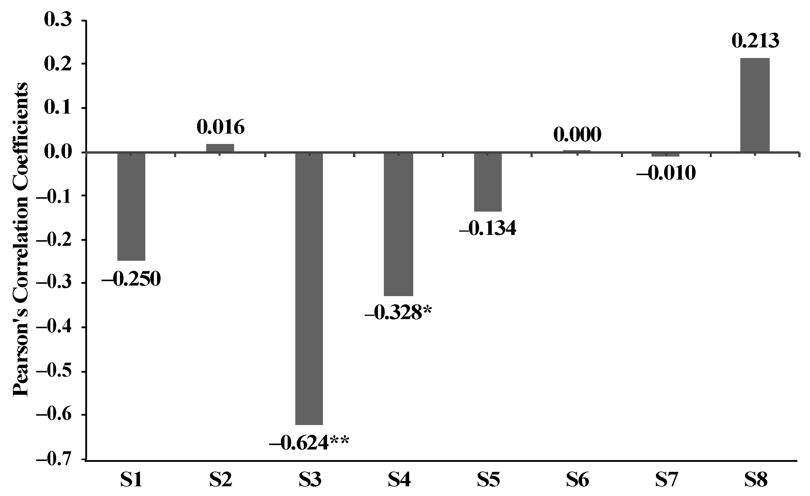
Precipitation is an important factor influencing the turbidity of the YZR, especially in the upper and middle sections. We found a lag of approximately one month for the effect of precipitation on turbidity. We also found the impact of precipitation type on turbidity change. Rainfall shows a positive correlation with turbidity in most stream sections. Snowfall, on the other hand, presents a slightly negative correlation with turbidity;
(5)
Vegetation plays a vital role in reducing turbidity at the upper and middle sections where vegetation coverage is limited.
Atmospheric correction and the removal of adjacency effects are critical but challenging for remote sensing-based turbidity monitoring of rivers on the Tibetan Plateau. Our study demonstrated that river turbidity could be derived successfully by the incorporation of measured reference radiance in the field and by careful atmospheric correction and water pixel extraction. Future study is recommended to optimize the time and locations of the in situ sampling collection with the consideration of stream types, accessibility, seasonal variation, and weather conditions to refine the turbidity models for different remote sensors. It is also worth exploring inherent optical properties and advanced models to develop more robust and generalized models and conducting additional hydrological analysis to understand the driving mechanisms in turbidity variations of the alpine rivers.

Author Contributions

M.S. and S.W. conceived and designed the method and the experiments. M.S., S.W., and Y.M. conducted the field experiments and investigations. M.S., Y.L., and M.T. performed data processing and analysis. M.S. wrote the original manuscript and Y.L. revised the manuscript. Y.L. conducted the project administration and funding acquisition. All authors have read and agreed to the published version of the manuscript.

Funding

This research was funded by a Summer Graduate Research Assistantship at the University of Tennessee. Funding for open access to this research was provided by the University of Tennessee’s Open Publishing Support Fund.

Data Availability Statement

The remote sensing data used in this study are openly available. The Landsat 5 and Landsat 8 imagery can be downloaded here: https://earthexplorer.usgs.gov/. The Sentinel-2 imagery can be downloaded here: https://scihub.copernicus.eu/dhus/#/home. The in situ measured data presented in this study are available on request from the authors.

Acknowledgments

The authors thank Youfa You, Weihua Liu and Jingshu Zhang, who helped with data collection and preprocessing. We also want to thank Haidong Li for providing valuable suggestions on the analysis of vegetation impacts. The Sentinel-2 images were provided by the European Space Agency Copernicus Open Access Hub and the Landsat series images were provided by the USGS Earth Resources Observation and Science Center. We are grateful to the two anonymous reviewers who provided helpful comments and suggestions to improve the manuscript.

Conflicts of Interest

The authors declare no conflict of interest.

References

  1. Li, J.; Fang, X.; Ma, H.; Zhu, J.; Pan, B.; Chen, H. Geomorphological and environmental evolution in the upper reaches of the Yellow River during the late Cenozoic. Sci. China Ser. D Earth Sci. 1996, 39, 380–390. [Google Scholar]
  2. Li, Y.; Liao, J.; Guo, H.; Liu, Z.; Shen, G. Patterns and potential drivers of dramatic changes in Tibetan lakes, 1972–2010. PLoS ONE 2014, 9, e111890. [Google Scholar] [CrossRef] [PubMed] [Green Version]
  3. Liao, C.; Liu, B.; Xu, Y.; Li, Y.; Li, H. Effect of topography and protecting barriers on revegetation of sandy land, Southern Tibetan Plateau. Sci. Rep. 2019, 9, 1–10. [Google Scholar] [CrossRef] [PubMed]
  4. Zhang, G.; Xie, H.; Kang, S.; Yi, D.; Ackley, S.F. Monitoring lake level changes on the Tibetan Plateau using ICESat altimetry data (2003–2009). Remote Sens. Environ. 2011, 115, 1733–1742. [Google Scholar] [CrossRef]
  5. Li, H.; Li, Y.; Gao, Y.; Zou, C.; Yan, S.; Gao, J. Human impact on vegetation dynamics around Lhasa, southern Tibetan plateau, China. Sustainability 2016, 8, 1146. [Google Scholar] [CrossRef] [Green Version]
  6. Zeng, C.; Zhang, F.; Lu, X.; Wang, G.; Gong, T. Improving sediment load estimations: The case of the Yarlung Zangbo River (the upper Brahmaputra, Tibet Plateau). Catena 2018, 160, 201–211. [Google Scholar] [CrossRef]
  7. Song, C.; Huang, B.; Ke, L.; Richards, K.S. Remote sensing of alpine lake water environment changes on the Tibetan Plateau and surroundings: A review. ISPRS J. Photogramm. Remote Sens. 2014, 92, 26–37. [Google Scholar] [CrossRef]
  8. Philpot, W.; Klemas, V. Remote Sensing of Coastal Pollutants Using Multispectral Data. In Proceedings of the Annual William T. Pecora Memorial Symposium on Remote Sensing, Sioux Falls, SD, USA, 10–15 January 1979. [Google Scholar]
  9. Ruhl, C.; Schoellhamer, D.; Stumpf, R.; Lindsay, C. Combined use of remote sensing and continuous monitoring to analyse the variability of suspended-sediment concentrations in San Francisco Bay, California. Estuar. Coast. Shelf Sci. 2001, 53, 801–812. [Google Scholar] [CrossRef]
  10. Shafique, N.A.; Fulk, F.; Autrey, B.C.; Flotemersch, J. Hyperspectral remote sensing of water quality parameters for large rivers in the Ohio River basin. In Proceedings of the First Interagency Conference on Research in the Watershed, Benson, AZ, USA, 27–30 October 2003; pp. 216–221. [Google Scholar]
  11. Fraser, R. Multispectral remote sensing of turbidity among Nebraska Sand Hills lakes. Int. J. Remote Sens. 1998, 19, 3011–3016. [Google Scholar] [CrossRef]
  12. Yu, X.; Lee, Z.; Shen, F.; Wang, M.; Wei, J.; Jiang, L.; Shang, Z. An empirical algorithm to seamlessly retrieve the concentration of suspended particulate matter from water color across ocean to turbid river mouths. Remote Sens. Environ. 2019, 235, 111491. [Google Scholar] [CrossRef]
  13. Liu, Y.; Islam, M.A.; Gao, J. Quantification of shallow water quality parameters by means of remote sensing. Prog. Phys. Geogr. 2003, 27, 24–43. [Google Scholar] [CrossRef]
  14. Kilham, N.E.; Roberts, D.; Singer, M.B. Remote sensing of suspended sediment concentration during turbid flood conditions on the Feather River, California—A modeling approach. Water Resour. Res. 2012, 48. [Google Scholar] [CrossRef] [Green Version]
  15. Petus, C.; Chust, G.; Gohin, F.; Doxaran, D.; Froidefond, J.-M.; Sagarminaga, Y. Estimating turbidity and total suspended matter in the Adour River plume (South Bay of Biscay) using MODIS 250-m imagery. Cont. Shelf Res. 2010, 30, 379–392. [Google Scholar] [CrossRef] [Green Version]
  16. Güttler, F.N.; Niculescu, S.; Gohin, F. Turbidity retrieval and monitoring of Danube Delta waters using multi-sensor optical remote sensing data: An integrated view from the delta plain lakes to the western–northwestern Black Sea coastal zone. Remote Sens. Environ. 2013, 132, 86–101. [Google Scholar] [CrossRef] [Green Version]
  17. Kallio, K.; Attila, J.; Härmä, P.; Koponen, S.; Pulliainen, J.; Hyytiäinen, U.-M.; Pyhälahti, T. Landsat ETM+ images in the estimation of seasonal lake water quality in boreal river basins. Environ. Manag. 2008, 42, 511–522. [Google Scholar] [CrossRef] [PubMed]
  18. Chen, Z.; Hu, C.; Muller-Karger, F. Monitoring turbidity in Tampa Bay using MODIS/Aqua 250-m imagery. Remote Sens. Environ. 2007, 109, 207–220. [Google Scholar] [CrossRef]
  19. Shen, F.; Suhyb Salama, M.; Zhou, Y.-X.; Li, J.-F.; Su, Z.; Kuang, D.-B. Remote-sensing reflectance characteristics of highly turbid estuarine waters—A comparative experiment of the Yangtze River and the Yellow River. Int. J. Remote Sens. 2010, 31, 2639–2654. [Google Scholar] [CrossRef]
  20. Doxaran, D.; Froidefond, J.-M.; Lavender, S.; Castaing, P. Spectral signature of highly turbid waters: Application with SPOT data to quantify suspended particulate matter concentrations. Remote Sens. Environ. 2002, 81, 149–161. [Google Scholar] [CrossRef]
  21. Gholizadeh, M.; Melesse, A. Study on spatiotemporal variability of water quality parameters in Florida Bay using remote sensing. J. Remote Sens. GIS 2017, 6, 1–11. [Google Scholar] [CrossRef]
  22. Hellweger, F.; Schlosser, P.; Lall, U.; Weissel, J. Use of satellite imagery for water quality studies in New York Harbor. Estuar. Coast. Shelf Sci. 2004, 61, 437–448. [Google Scholar] [CrossRef]
  23. Chen, S.; Fang, L.; Zhang, L.; Huang, W. Remote sensing of turbidity in seawater intrusion reaches of Pearl River Estuary–A case study in Modaomen water way, China. Estuar. Coast. Shelf Sci. 2009, 82, 119–127. [Google Scholar] [CrossRef]
  24. Qiu, J. China: The third pole. Nature 2008, 454, 393–396. [Google Scholar] [CrossRef] [PubMed] [Green Version]
  25. Mingyue, H.; Linjuan, P.; Dingzhi, Z.; Linghua, Q. Spatial interpolation of meteorological variables in yarlung zangbo river basin. J. Beijing Norm. Univ. (Nat. Sci.) 2012, 48, 449–452. [Google Scholar]
  26. Zheng, W.; Kang, S.; Feng, X.; Zhang, Q.; Li, C. Mercury speciation and spatial distribution in surface waters of the Yarlung Zangbo River, Tibet. Chin. Sci. Bull. 2010, 55, 2697–2703. [Google Scholar] [CrossRef]
  27. Nan, S.; Li, J.; Zhang, L.; An, R.; Pu, X.; Huang, W. Distribution Characteristics of Phosphorus in the Yarlung Zangbo River Basin. Water 2018, 10, 913. [Google Scholar] [CrossRef] [Green Version]
  28. Huang, X.; Sillanpää, M.; Gjessing, E.; Peräniemi, S.; Vogt, R. Water quality in the southern Tibetan Plateau: Chemical evaluation of the Yarlung Tsangpo (Brahmaputra). River Res. Appl. 2011, 27, 113–121. [Google Scholar] [CrossRef]
  29. Huang, X.; Sillanpää, M.; Duo, B.; Gjessing, E.T. Water quality in the Tibetan Plateau: Metal contents of four selected rivers. Environ. Pollut. 2008, 156, 270–277. [Google Scholar] [CrossRef]
  30. Huang, Z.; Lin, B.; Sun, J.; Luozhu, N.; Da, P.; Dawa, J. Suspended Sediment Transport Responses to Increasing Human Activities in a High-Altitude River: A Case Study in a Typical Sub-Catchment of the Yarlung Tsangpo River. Water 2020, 12, 952. [Google Scholar] [CrossRef] [Green Version]
  31. Ming-Hui, H.; Stallard, R.; Edmond, J. Major ion chemistry of some large Chinese rivers. Nature 1982, 298, 550–553. [Google Scholar] [CrossRef]
  32. Huang, X.; Sillanpää, M.; Gjessing, E.T.; Vogt, R.D. Water quality in the Tibetan Plateau: Major ions and trace elements in the headwaters of four major Asian rivers. Sci. Total Environ. 2009, 407, 6242–6254. [Google Scholar] [CrossRef]
  33. Shi, X.; Zhang, F.; Lu, X.; Wang, Z.; Gong, T.; Wang, G.; Zhang, H. Spatiotemporal variations of suspended sediment transport in the upstream and midstream of the Yarlung Tsangpo River (the upper Brahmaputra), China. Earth Surf. Process. Landf. 2018, 43, 432–443. [Google Scholar] [CrossRef]
  34. Zhang, Y.; Sillanpää, M.; Li, C.; Guo, J.; Qu, B.; Kang, S. River water quality across the Himalayan regions: Elemental concentrations in headwaters of Yarlung Tsangbo, Indus and Ganges River. Environ. Earth Sci. 2015, 73, 4151–4163. [Google Scholar] [CrossRef]
  35. Li, H.; Li, Y.; Shen, W.; Li, Y.; Lin, J.; Lu, X.; Xu, X.; Jiang, J. Elevation-dependent vegetation greening of the Yarlung Zangbo River basin in the southern Tibetan Plateau, 1999–2013. Remote Sens. 2015, 7, 16672–16687. [Google Scholar] [CrossRef] [Green Version]
  36. Chettri, N.; Tsering, K.; Shrestha, A.; Sharma, E. Ecological vulnerability to climate change in the mountains: A case study from the Eastern Himalaya. In Floristic Diversity in Himalaya Hotspot Region; Bishen Singh Mahendra Pal Singh: Dehra Dun, India, 2018. [Google Scholar]
  37. Zhong, L.; Ma, Y.; Fu, Y.; Pan, X.; Hu, W.; Su, Z.; Salama, M.S.; Feng, L. Assessment of soil water deficit for the middle reaches of Yarlung-Zangbo River from optical and passive microwave images. Remote Sens. Environ. 2014, 142, 1–8. [Google Scholar] [CrossRef]
  38. Liu, Z.; Tian, L.; Yao, T. Variations of δ~(18)O in Precipitation of the Yarlung Zangbo River Basin. Acta Geogr. Sin. Chin. Ed. 2007, 62, 517. [Google Scholar]
  39. Wang, X.; Zhong, X.; Liu, S.; Liu, J.; Wang, Z.; Li, M. Regional assessment of environmental vulnerability in the Tibetan Plateau: Development and application of a new method. J. Arid Environ. 2008, 72, 1929–1939. [Google Scholar] [CrossRef]
  40. Wang, L.; Zhang, F.; Fu, S.; Shi, X.; Chen, Y.; Jagirani, M.D.; Zeng, C. Assessment of soil erosion risk and its response to climate change in the mid-Yarlung Tsangpo River region. Environ. Sci. Pollut. Res. 2020, 27, 607–621. [Google Scholar] [CrossRef]
  41. Wei, X.-H.; Yang, P.; Dong, G.-R. Agricultural development and farmland desertification in middle “One River and Its Two Branches” River basin of Tibet. J. Desert Res. 2004, 24, 196–200. [Google Scholar]
  42. Chinese Research Academy of Environmental Sciences. State Environment Protection Key Laboratory of Ecological Effects and Risk Assessment of Chemicals. Available online: http://www.craes.cn/en/ (accessed on 30 December 2020).
  43. Kitchener, B.G.; Wainwright, J.; Parsons, A.J. A review of the principles of turbidity measurement. Prog. Phys. Geogr. 2017, 41, 620–642. [Google Scholar] [CrossRef] [Green Version]
  44. Spectroradiometer, H. User’s Guide Version 4.05; Analytical Spectral Devices: Boulder, CO, USA, 2005. [Google Scholar]
  45. Sivasankar, T.; Borah, S.B.; Das, R.; Raju, P. An Investigation on Sudden Change in Water Quality of Brahmaputra River Using Remote Sensing and GIS. Natl. Acad. Sci. Lett. 2020, 43, 619–623. [Google Scholar] [CrossRef]
  46. Salama, M.; Dekker, A.; Su, Z.; Mannaerts, C.; Verhoef, W. Deriving inherent optical properties and associated inversion-uncertainties in the Dutch Lakes. Hydrol. Earth Syst. Sci. 2009, 13, 1113. [Google Scholar] [CrossRef] [Green Version]
  47. Thiemann, S.; Kaufmann, H. Determination of chlorophyll content and trophic state of lakes using field spectrometer and IRS-1C satellite data in the Mecklenburg Lake District, Germany. Remote Sens. Environ. 2000, 73, 227–235. [Google Scholar] [CrossRef]
  48. Huang, W.; Huang, J.; Wang, X.; Wang, F.; Shi, J. Comparability of red/near-infrared reflectance and NDVI based on the spectral response function between MODIS and 30 other satellite sensors using rice canopy spectra. Sensors 2013, 13, 16023–16050. [Google Scholar] [CrossRef] [PubMed]
  49. USGS. EarthExplorer. Available online: https://earthexplorer.usgs.gov/ (accessed on 30 December 2020).
  50. European Space Agency. Copernicus Open Access Hub. Available online: https://scihub.copernicus.eu/dhus/#/home (accessed on 30 December 2020).
  51. Gascon, F.; Ramoino, F. Sentinel-2 Data Exploitation with ESA’s Sentinel-2 Toolbox. In Proceedings of the 19th European Geosciences Union (EGU) General Assembly 2017, Vienna, Austria, 23–28 April 2017. [Google Scholar]
  52. Louis, J.; Debaecker, V.; Pflug, B.; Main-Knorn, M.; Bieniarz, J.; Mueller-Wilm, U.; Cadau, E.; Gascon, F. Sentinel-2 Sen2Cor: L2A processor for users. In Proceedings of the Proceedings Living Planet Symposium 2016, Prague, Czech Republic, 9–13 May 2016; pp. 1–8. [Google Scholar]
  53. Vibhute, A.D.; Kale, K.; Dhumal, R.K.; Mehrotra, S. Hyperspectral imaging data atmospheric correction challenges and solutions using QUAC and FLAASH algorithms. In Proceedings of the 2015 International Conference on Man and Machine Interfacing (MAMI), Bhubaneswar, India, 17–19 December 2015; pp. 1–6. [Google Scholar]
  54. Singh, K.V.; Setia, R.; Sahoo, S.; Prasad, A.; Pateriya, B. Evaluation of NDWI and MNDWI for assessment of waterlogging by integrating digital elevation model and groundwater level. Geocarto Int. 2015, 30, 650–661. [Google Scholar] [CrossRef]
  55. Xu, H. Modification of normalised difference water index (NDWI) to enhance open water features in remotely sensed imagery. Int. J. Remote Sens. 2006, 27, 3025–3033. [Google Scholar] [CrossRef]
  56. Peng, S.; Ding, Y.; Liu, W.; Li, Z. 1 km monthly temperature and precipitation dataset for China from 1901 to 2017. Earth Syst. Sci. Data 2019, 11, 1931–1946. [Google Scholar] [CrossRef] [Green Version]
  57. Google Earth Engine. Landsat 8 Collection 1 Tier 1 Annual NDVI Composite. 1 January 2013–1 January 2021. Available online: https://explorer.earthengine.google.com/#detail/LANDSAT%2FLC08%2FC01%2FT1_ANNUAL_NDVI (accessed on 6 January 2021).
  58. Google Earth Engine. Landsat 5 TM Collection 1 Tier 1 Annual NDVI Composite. 1 January 1984–1 January 2013. Available online: https://explorer.earthengine.google.com/#detail/LANDSAT%2FLT05%2FC01%2FT1_ANNUAL_NDVI (accessed on 6 January 2021).
  59. Abyaneh, H.Z. Evaluation of multivariate linear regression and artificial neural networks in prediction of water quality parameters. J. Environ. Health Sci. Eng. 2014, 12, 40. [Google Scholar] [CrossRef] [Green Version]
  60. Schneider, A.; Hommel, G.; Blettner, M. Linear regression analysis: Part 14 of a series on evaluation of scientific publications. Dtsch. Ärzteblatt Int. 2010, 107, 776. [Google Scholar]
  61. IBM. SPSS 23.0. Available online: https://www.ibm.com/support/pages/downloading-ibm-spss-statistics-23 (accessed on 30 December 2020).
  62. R 3.5.2. Available online: https://cran.r-project.org/bin/windows/base/old/3.5.2/ (accessed on 30 December 2020).
  63. Dai, X.; Zhou, Y.; Ma, W.; Zhou, L. Influence of spatial variation in land-use patterns and topography on water quality of the rivers inflowing to Fuxian Lake, a large deep lake in the plateau of southwestern China. Ecol. Eng. 2017, 99, 417–428. [Google Scholar] [CrossRef]
  64. Bonansea, M.; Rodriguez, M.C.; Pinotti, L.; Ferrero, S. Using multi-temporal Landsat imagery and linear mixed models for assessing water quality parameters in Río Tercero reservoir (Argentina). Remote Sens. Environ. 2015, 158, 28–41. [Google Scholar] [CrossRef]
  65. Du, J.; Shi, C.-x. Modeling and analysis of effects of precipitation and vegetation coverage on runoff and sediment yield in Jinsha River Basin. Water Sci. Eng. 2013, 6, 44–58. [Google Scholar]
  66. Langbein, W.B.; Schumm, S.A. Yield of sediment in relation to mean annual precipitation. EosTrans. Am. Geophys. Union 1958, 39, 1076–1084. [Google Scholar] [CrossRef] [Green Version]
  67. Matthews, M.W. A current review of empirical procedures of remote sensing in inland and near-coastal transitional waters. Int. J. Remote Sens. 2011, 32, 6855–6899. [Google Scholar] [CrossRef]
  68. Palmer, S.C.; Kutser, T.; Hunter, P.D. Remote Sensing of Inland Waters: Challenges, Progress and Future Directions. Remote Sens. Environ. 2015, 157, 1–8. [Google Scholar] [CrossRef] [Green Version]
  69. Kuhn, C.; de Matos Valerio, A.; Ward, N.; Loken, L.; Sawakuchi, H.O.; Kampel, M.; Richey, J.; Stadler, P.; Crawford, J.; Striegl, R. Performance of Landsat-8 and Sentinel-2 surface reflectance products for river remote sensing retrievals of chlorophyll-a and turbidity. Remote Sens. Environ. 2019, 224, 104–118. [Google Scholar] [CrossRef] [Green Version]
  70. Sha, Y.; Li, W.; Fan, J.; Cheng, G. Determining critical support discharge of a riverhead and river network analysis: Case studies of Lhasa River and Nyangqu River. Chin. Geogr. Sci. 2016, 26, 456–465. [Google Scholar] [CrossRef] [Green Version]
  71. Guo, B.; Jiang, L.; Ge, D.; Shang, M. Driving mechanism of vegetation coverage change in the Yarlung Zangbo River Basin under the stress of global warming. J. Trop. Subtrop. Bot. 2017, 25, 209–217. [Google Scholar]
  72. Bing, C.Y.H.L.X.; Jun, S.P. Variation in ndvi driven by climate factors across china, 1983–1992. Acta Phytoecol. Sin. 2001, 25, 716–720. [Google Scholar]
  73. Gao, G.; Zhang, J.; Liu, Y.; Ning, Z.; Fu, B.; Sivapalan, M. Spatio-temporal patterns of the effects of precipitation variability and land use/cover changes on long-term changes in sediment yield in the Loess Plateau, China. Hydrol. Earth Syst. Sci. 2017, 21, 4363–4378. [Google Scholar] [CrossRef] [Green Version]
Figure 1. The location of study area and the sample sites of in situ measurements. (a) Location and the elevation map of the Yarlung Zangbo River Basin in China; (b) sample sites near the confluence of Lhasa River; (c) sample sites near the confluence of Nyang River.
Remotesensing 13 00182 g001
Figure 2. Division of the stream sections. The blue shaded region illustrates the middle reaches of the Yarlung Zangbo River (YZR) in this study that were further divided into eight sections from S1 to S8 by the blue dash lines.
Remotesensing 13 00182 g002
Figure 3. Boxplots of water sample turbidity in different regions.
Remotesensing 13 00182 g003
Figure 4. Spectral curves of water samples with different turbidity values in the YZR. The measured turbidity values were marked for each spectral curve.
Remotesensing 13 00182 g004
Figure 5. Relative errors of modeling samples.
Remotesensing 13 00182 g005
Figure 6. Scatter plots of measured and estimated turbidity values based on the s-curve models. Left panels (a,c,e) are for the model development (n = 24) and right panels (b,d,f) for the validation (n = 12). (a,b) are s-curve models for Sentinel-2 MSI images, (c,d) for Landsat 8 OLI, and (e,f) for Landsat 5 TM, respectively.
Remotesensing 13 00182 g006
Figure 7. Spatial pattern of turbidity changes along the middle reaches of the YZR.
Remotesensing 13 00182 g007
Figure 8. Seasonal changes of turbidity in the middle reaches of the YZR.
Remotesensing 13 00182 g008
Figure 9. Annual changes of turbidity in the middle reaches of the YZR.
Remotesensing 13 00182 g009
Figure 10. Temporal turbidity changes with precipitation. (a) Seasonal change of monthly mean turbidity and precipitation. (b) Interannual change of yearly mean turbidity and precipitation.
Remotesensing 13 00182 g010
Figure 11. Spatial change of multiyear average turbidity and precipitation at different sections.
Remotesensing 13 00182 g011
Figure 12. Annual Normalized Difference Vegetation Index (NDVI) and turbidity change in different sections.
Remotesensing 13 00182 g012
Figure 13. Pearson’s correlation between the turbidity values in the tributaries and the mainstream. The numbers on each shaded box are Pearson’s correlation coefficients. ** marks the significant correlation at the 0.01 level (2-tailed) and * marks the significant correlation at the 0.05 level (2-tailed).
Remotesensing 13 00182 g013
Figure 14. Correlation between turbidity and precipitation in specific periods.
Remotesensing 13 00182 g014
Figure 15. Correlation between turbidity and annual NDVIs. * means that the correlation is significant at the 0.05 level (2-tailed). ** means that correlation is significant at the 0.01 level (2-tailed).
Remotesensing 13 00182 g015
Table 1. Main technical specifications of the optical satellite images used in this study.
SensorBandsSpatial Resolution
Landsat 5, Thematic Mapper (TM)Band 1 Blue (450–520 nm), Band 2 Green (520–600 nm), Band 3 Red (630–690 nm), Band 4 NIR (760–900 nm)30 m
Landsat 8, Operational Land Imager (OLI)Band 2 Blue (450–515 nm), Band 3 Green (525–600 nm), Band 4 Red (630–680 nm), Band 5 NIR (845–885 nm)30 m
Sentinel-2, Multispectral Instrument (MSI)Band 2 Blue (459–525 nm), Band 3 Green (542–578 nm), Band 4 Red (649–680 nm), Band 8 NIR (779–885 nm)10 m
Band 5 Red Edge (697–712 nm), Band 6 Red Edge (733–748 nm), Band 7 Red Edge (773–793 nm), Band 8a NIR (854–875 nm)20 m
NIR: Near Infrared.
Table 2. Number of selected images.
SensorsLandsat 5 TMLandsat 8 OLISentinel-2 MSI
Year200720082009201020112013201420152016201720162017
January82878/424142
February25878/432253
March77713/033402
April738641213202
May424231100224
June114130200102
July120000000103
August100122002101
September111253010202
October144231241233
November099943546646
December0105906545548
Total334658474317252226292238
/: No images available. 0: No clear and cloud-free images.
Table 3. Regression models used for deriving turbidity.
Model FormatsEquationDescription
LinearY = b + a × XLinear model grows at a constant rate.
LogarithmicY = b + a × ln(X)Logarithmic model grows very rapidly followed by slower growth to infinity.
InverseY = b + a/XInverse function is also known as reciprocal function. Its vertical asymptote is x = 0 and horizonal asymptote is y = b.
QuadraticY = b + a1 × X + a2 × X2The graph of a univariate quadratic function is a parabola which opens upwards when a1 is positive and is symmetric at x = −a2/(2 × a1).
CubicY = b + a1 × X + a2 × X2 + a3 × X3Cubic model delineates polynomial growth at the 3rd order.
Exponentialln(Y) = ln(b) + a × XExponential growth passes through (0, b) and keeps increasing to infinity.
Powerln(Y) = ln(b) + a × ln(X)Power curve passes through (0,0) and (1, b). As the power increases, the graphs flatten somewhat near the origin and become steeper away from the origin.
S-curveln(Y) = b + a/XS-curve model is a sigmoid function with an “S”-shape like the logistic model. It first grows slowly, then moderately and finally slowly approaches an asymptote.
a, b are parameters to be estimated.
Table 4. Pearson’s correlation between measured turbidity and spectral indices of visible and near-infrared reflectance.
Landsat 5 TMLandsat 8 OLISentinel-2 MSI
Blue−0.145−0.151−0.132
Green−0.023−0.040−0.042
Red0.1100.1020.120
NIR0.2080.1870.212
NIR/Blue0.669 **0.591 **0.667 **
NIR/Green0.548 **0.459 **0.575 **
NIR/Red0.413 *0.2920.417 *
Red/Blue0.696 **0.697 **0.704 *
Red/Green0.761 **0.759 **0.759 **
Green/Blue0.733 **0.719 **0.710 **
(NIR − Blue)/(NIR + Blue)0.650 **0.623 **0.687 **
(NIR − Green)/(NIR + Green)0.550 **0.485 **0.571 **
(NIR − Red)/(NIR + Red)0.445 *0.339 *0.335 *
(Red − Blue)/(Red + Blue)0.690 **0.692 **0.699 **
(Red − Green)/(Red + Green)0.727 **0.716 **0.708
(Green − Blue)/(Green + Blue)0.708 **0.704 **0.712 **
*: Correlation is significant at the 0.05 level (2-tailed). **: Correlation is significant at the 0.01 level (2-tailed). Blue: Band 1 for Thematic Mapper (TM), Band 2 for Operational Land Imager (OLI), and Band 2 for Multispectral Imager (MSI). Green: Band 2 for TM, Band 3 for OLI, and Band 3 for MSI. Red: Band 3 for TM, Band 4 for OLI, and Band 4 for MSI. NIR: Near-infrared band. Band 4 for TM, Band 5 for OLI, and Band 8 for MSI.
Table 5. Pearson’s correlation between measured turbidity and spectral indices of narrow bands of Sentinel-2 MSI imagery.
Red Edge1
(Band 5)
Red Edge2
(Band 6)
Red Edge3
(Band 7)
Near-Infrared
(Band 8a)
Single band0.1380.2340.2450.187
Band ratio with Blue band (Band 2)0.667 **0.665 **0.654 **0.460 *
Band ratio with Green band (Band 3)0.737 **0.740 **0.729 **0.569 **
Band ratio with Red band (Band 4)0.335 *0.540 **0.539 **0.263
*: Correlation is significant at the 0.05 level (2-tailed); **: Correlation is significant at the 0.01 level (2-tailed).
Table 6. The performances of turbidity models for different sensors.
SensorsModel FormatsEquations 1R2RMSMRE
Sentinel-2 MSILinearY = −303.725 + 409.219 × X0.62234.7560.992
LogarithmicY = 105.062 + 352.143 × ln(X)0.59635.9201.134
InverseY = 399.117 − 295.022/X0.56337.3491.309
QuadraticY= 337.271 − 1051.336 × X + 818.009 × X20.66132.9200.679
CubicY = 35.391 − 385.724*X2 + 435.681*X30.66132.9100.731
Exponentialln(Y) = −5.298 + 9.814 × X0.76440.4060.497
Powerln(Y) = 4.528 + 8.638 × ln(X)0.76636.0910.488
S-curveln(Y) = 11.918 − 7.4/X0.75734.5500.498
Landsat 8 OLILinearY = −346.292 + (445.641 × X)0.60935.3181.031
LogarithmicY = 99.470 + (391.316 × ln(X))0.58236.5201.171
InverseY = 434.836 + (−335.683/X)0.54937.9331.338
QuadraticY = 535.137 + (−1517.783 × X) + (1078.271 × X2)0.66132.8900.630
CubicY = 253.884 + (−558.206 × X) + (0 × X2) + (399.496 × X3)0.66132.8810.667
Exponentialln(Y) = ln(0.002) + (10.798 × X)0.76539.7050.489
Powerln(Y) = ln(81.066) + (9.687 × ln(X))0.76335.8730.485
S-curveln(Y) = 12.886 + (−8.488/X)0.75134.6260.504
Landsat 5 TMLinearY = −379.185 + (483.082 × X)0.61035.2811.024
LogarithmicY = 103.605 + (426.526 × ln(X))0.58736.2961.145
InverseY = 472.612 + (−369.664/X)0.56037.4871.289
QuadraticY = 637.447 + (−1778.314 × X) + (1242.904 × X2)0.65733.0940.651
CubicY = 114.834 + (0 × X) + (−754.652 × X2) + (741.251 × X3)0.65733.0740.700
Exponentialln(Y) = ln(0.001) + (11.676 × X)0.76239.3110.494
Powerln(Y) = ln(89.525 + (10.507 × ln(X))0.76236.0650.487
S-curveln(Y) = 13.77 + (−9.28/X)0.75434.7500.494
1: X is the reflectance ratio between the equivalent red and green bands. For TM, X equals to Band 3/Band 2. For OLI, X equals to Band 4/Band 3. For MSI, X equals to Band 4/Band 3. Y is the in situ measured turbidity (NTU).
Table 7. Mean relative error (MRE) of different turbidity groups (taking Sentinel-2 models as an example.).
Model FormatsMRE (Overall)MRE (Turbidity >30 NTU)
Linear0.9920.221
Logarithmic1.1340.222
Inverse1.3090.221
Quadratic0.6790.219
Cubic0.7310.217
Exponential0.4970.28
Power0.4880.251
S-Curve0.4980.233
Table 8. Validation of the s-curve models.
SensorsSentinel-2 MSILandsat 8 OLILandsat 5 TM
MRE (All validation samples)2.7452.7142.741
MRE (Validation samples of turbidity > 30 NTU)0.1890.1920.193
RMS10.77611.07411.055
Table 9. Correlation coefficients of turbidity and precipitation.
Turbidity~ PrecipitationTurbidity~
Precipitation One Month Earlier
S10.865 **0.843 **
S20.790 **0.851 **
S30.471 **0.753 **
S40.670 **0.541 **
S50.608 **0.668 **
S60.752 **0.835 **
S70.494 **0.368 **
S80.2800.293
** Correlation is significant at the 0.01 level (2-tailed).
Publisher’s Note: MDPI stays neutral with regard to jurisdictional claims in published maps and institutional affiliations.

