Exploring the Relationship between River Discharge and Coastal Erosion: An Integrated Approach Applied to the Pisa Coastal Plain (Italy)


Abstract
:1. Introduction
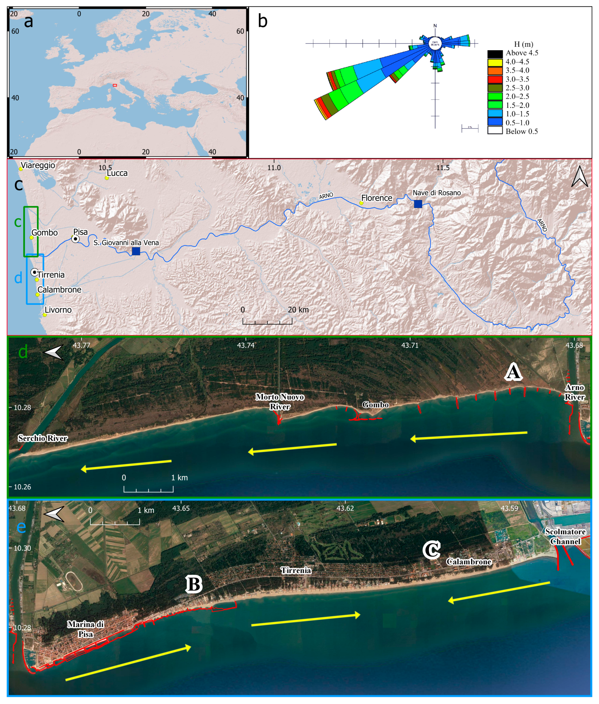
2. Study Area
3. Materials and Methods
4. Results
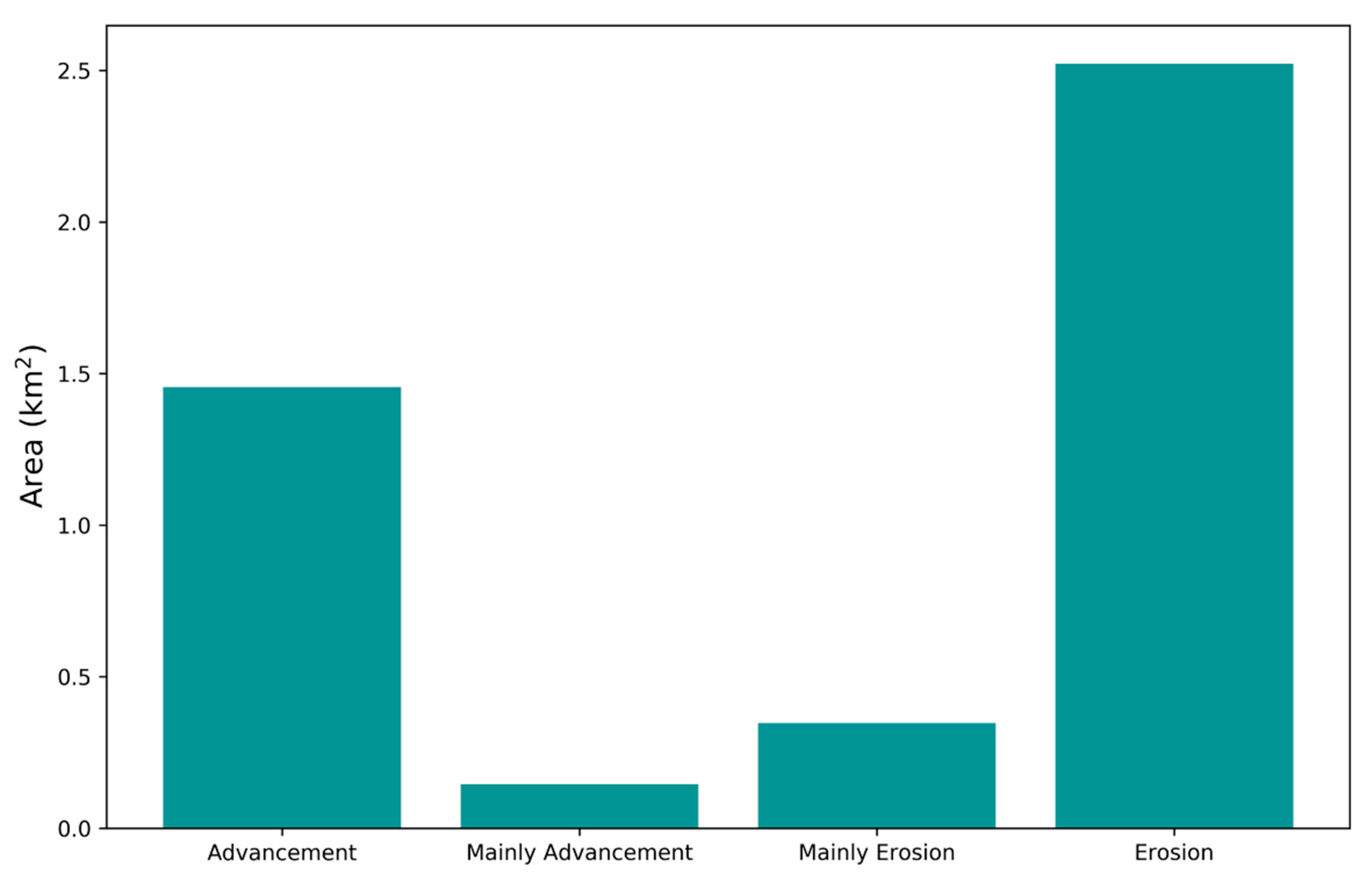
4.1. Shoreline GIS Analysis
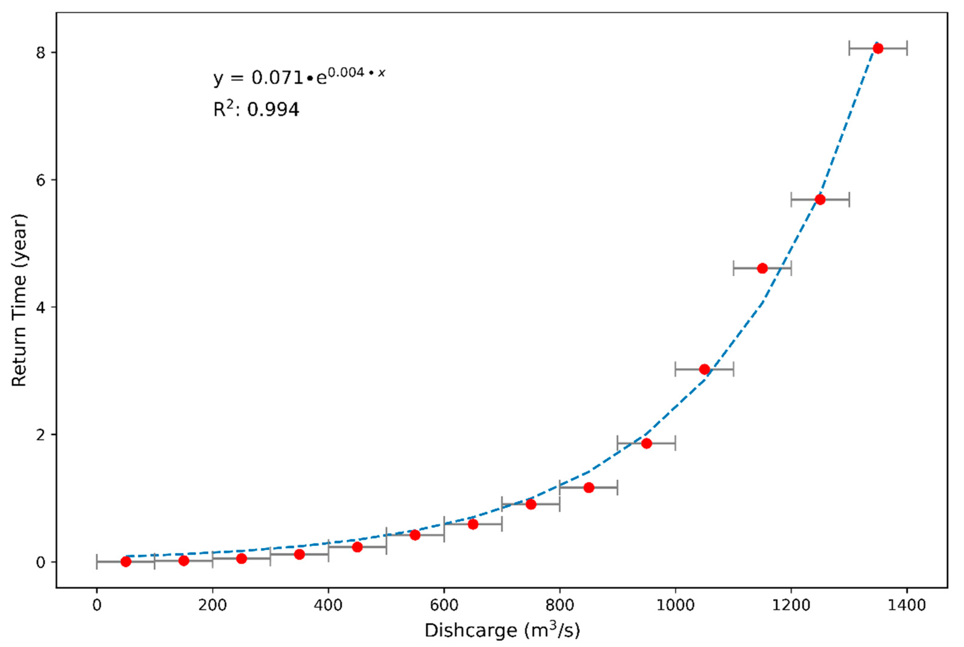
4.2. Discharge Data Analysis
4.3. Remote Sensing Analysis
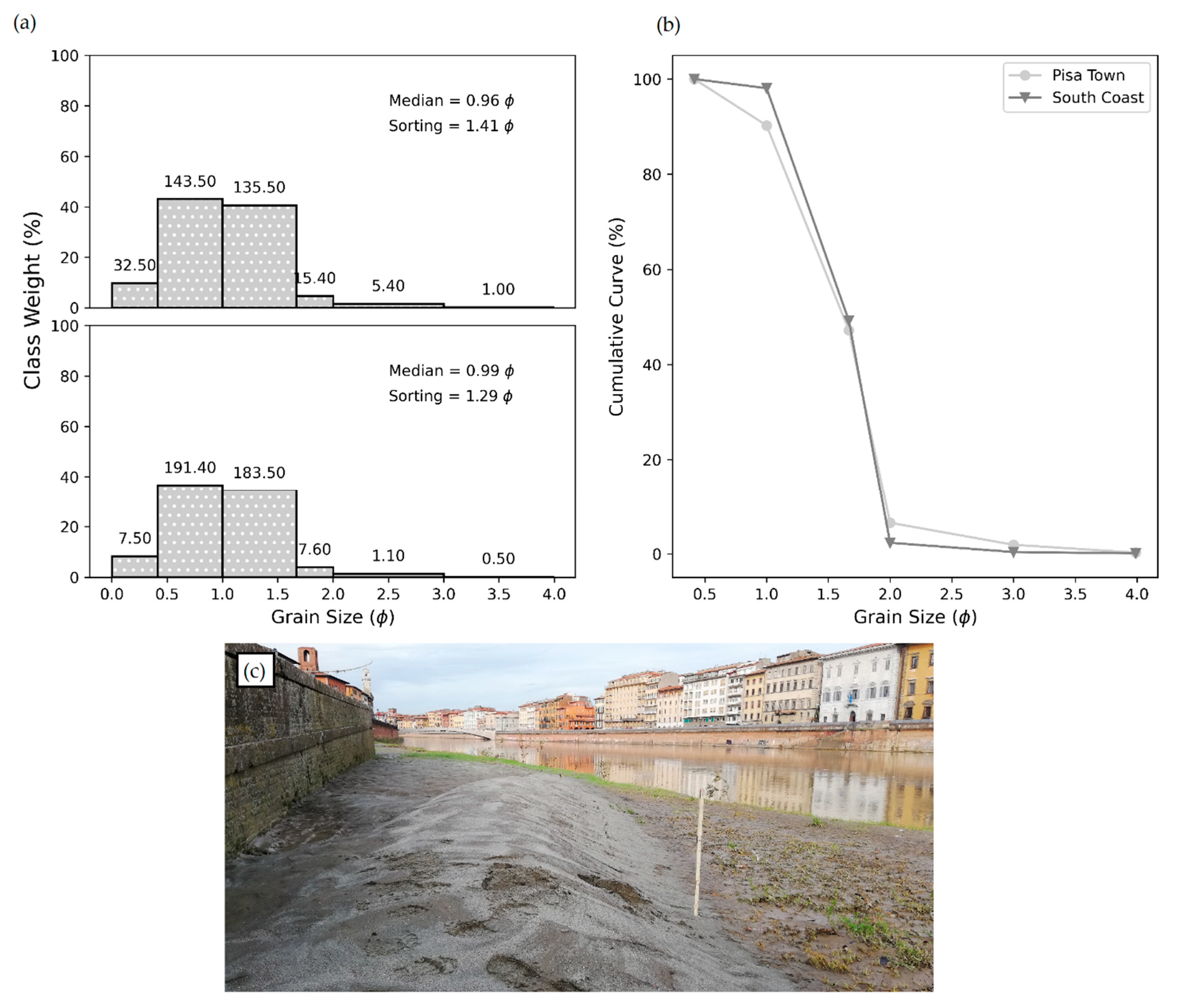
4.4. Post-Flood Field Investigations
5. Discussions
6. Conclusions
Supplementary Materials
Author Contributions
Funding
Institutional Review Board Statement
Informed Consent Statement
Data Availability Statement
Acknowledgments
Conflicts of Interest
References
- Lenôtre, N.; Thierry, P.; Batkowski, D.; Vermeersch, F. EUROSION Project The Coastal Erosion Layer. WP 2004, 2, 45. [Google Scholar]
- Luijendijk, A.; Hagenaars, G.; Ranasinghe, R.; Baart, F.; Donchyts, G.; Aarninkhof, S. The state of the world’s beaches. Sci. Rep. 2018, 8, 6641. [Google Scholar] [CrossRef]
- IPCC. Global warming of 1.5 °C. In An IPCC Special Report on the Impacts of Global Warming of 1.5 °C Above Pre-Industrial Levels and Related Global Greenhouse Gas Emission Pathways, in the Context of Strengthening the Global Response to the Threat of Climate Change, Sustainable Development, and Efforts to Eradicate Poverty; IPCC: Geneva, Switzerland, 2018. [Google Scholar]
- Bird, E.C.F. Coastline Changes: A Global Review; Wiley: Chichester, UK; New York, NY, USA, 1985; ISBN 978-0-471-90646-9. [Google Scholar]
- Mentaschi, L.; Vousdoukas, M.I.; Pekel, J.-F.; Voukouvalas, E.; Feyen, L. Global long-term observations of coastal erosion and accretion. Sci. Rep. 2018, 8, 12876. [Google Scholar] [CrossRef] [Green Version]
- IPCC. Climate Change 2013 The Physical Science Basis; Stocker, T.F., Ed.; IPCC: Geneva, Switzerland, 2013. [Google Scholar]
- Toimil, A.; Camus, P.; Losada, I.J.; Le Cozannet, G.; Nicholls, R.J.; Idier, D.; Maspataud, A. Climate change-driven coastal erosion modelling in temperate sandy beaches: Methods and uncertainty treatment. Earth Sci. Rev. 2020, 202, 103110. [Google Scholar] [CrossRef]
- Besset, M.; Anthony, E.J.; Bouchette, F. Multi-decadal variations in delta shorelines and their relationship to river sediment supply: An assessment and review. Earth Sci. Rev. 2019, 193, 199–219. [Google Scholar] [CrossRef] [Green Version]
- Anthony, E.J.; Marriner, N.; Morhange, C. Human influence and the changing geomorphology of Mediterranean deltas and coasts over the last 6000years: From progradation to destruction phase? Earth Sci. Rev. 2014, 139, 336–361. [Google Scholar] [CrossRef]
- Anthony, E.J. Sand and gravel supply from rivers to coasts: A review from a Mediterranean perspective. Atti Soc. Toscana Sci. Nat. Mem. Ser. A 2018, 125, 13–33. [Google Scholar]
- Anfuso, G.; Pranzini, E.; Vitale, G. An integrated approach to coastal erosion problems in northern Tuscany (Italy): Littoral morphological evolution and cell distribution. Geomorphology 2011, 129, 204–214. [Google Scholar] [CrossRef]
- Blöschl, G.; Hall, J.; Viglione, A.; Perdigão, R.A.P.; Parajka, J.; Merz, B.; Lun, D.; Arheimer, B.; Aronica, G.T.; Bilibashi, A.; et al. Changing climate both increases and decreases European river floods. Nature 2019, 573, 108–111. [Google Scholar] [CrossRef]
- Petropoulos, G.P.; Ireland, G.; Barrett, B. Surface soil moisture retrievals from remote sensing: Current status, products & future trends. Phys. Chem. EarthParts A B C 2015, 83–84, 36–56. [Google Scholar]
- Billi, P.; Fazzini, M. Global change and river flow in Italy. Glob. Planet. Chang. 2017, 155, 234–246. [Google Scholar] [CrossRef]
- Degeai, J.-P.; Bertoncello, F.; Vacchi, M.; Augustin, L.; de Moya, A.; Ardito, L.; Devillers, B. A new interpolation method to measure delta evolution and sediment flux: Application to the late Holocene coastal plain of the Argens River in the western Mediterranean. Mar. Geol. 2020, 424, 106159. [Google Scholar] [CrossRef]
- Pratellesi, M.; Ciavola, P.; Ivaldi, R.; Anthony, E.J.; Armaroli, C. River-mouth geomorphological changes over > 130 years (1882–2014) in a small Mediterranean delta: Is the Magra delta reverting to an estuary? Mar. Geol. 2018, 403, 215–224. [Google Scholar] [CrossRef]
- Ericson, J.; Vörösmarty, C.; Dingman, S.; Ward, L.; Meybeck, M. Effective sea-level rise and deltas: Causes of change and human dimension implications. Glob. Planet. Chang. 2006, 50, 63–82. [Google Scholar] [CrossRef]
- Syvitski, J.P.M.; Kettner, A.J.; Overeem, I.; Hutton, E.W.H.; Hannon, M.T.; Brakenridge, G.R.; Day, J.; Vörösmarty, C.; Saito, Y.; Giosan, L.; et al. Sinking deltas due to human activities. Nat. Geosci. 2009, 2, 681–686. [Google Scholar] [CrossRef]
- Tessler, Z.D.; Vörösmarty, C.J.; Grossberg, M.; Gladkova, I.; Aizenman, H. A global empirical typology of anthropogenic drivers of environmental change in deltas. Sustain. Sci. 2016, 11, 525–537. [Google Scholar] [CrossRef] [Green Version]
- Toniolo, A.R. Sulle Variazioni di Spiaggia a Foce d’Arno (Marina di Pisa) Dalla Fine del Secolo XViii ai Nostri Giorni: Studio Storico Fisiografico; Comune di Pisa, Ed.; Tipografia Municipale: Pisa, Italy, 1910. [Google Scholar]
- Borgh, L. Apporto Allo Studio Sulle Cause di Variazione del Litorale Pisano; Comune di Pisa: Pisa, Italy, 1970. [Google Scholar]
- Bini, M.; Casarosa, N.; Ribolini, A. L’evoluzione diacronica della linea di riva del litorale Pisano (1938–2004) sulla base del confront di immagini aeree georeferenziate. Atti Della Soc. Toscana Sci. Nat. Mem. Ser. A 2008, 113, 1–12. [Google Scholar]
- Pozzebon, A.; Cappelli, I.; Mecocci, A.; Bertoni, D.; Sarti, G.; Alquini, F. A wireless sensor network for the real-time remote measurement of aeolian sand transport on sandy beaches and dunes. Sensors 2018, 18, 820. [Google Scholar] [CrossRef] [Green Version]
- Besset, M.; Anthony, E.J.; Sabatier, F. River delta shoreline reworking and erosion in the Mediterranean and Black Seas: The potential roles of fluvial sediment starvation and other factors. Elem. Sci. Anthr. 2017, 5, 54. [Google Scholar] [CrossRef] [Green Version]
- Grottoli, E.; Bertoni, D.; Pozzebon, A.; Ciavola, P. Influence of particle shape on pebble transport in a mixed sand and gravel beach during low energy conditions. Ocean Coast. Manag. 2019, 169, 171–181. [Google Scholar] [CrossRef]
- Palla, B. Variazioni della linea di riva tra i Fiumi Arno e Serchio (Tenuta di S. Rossore—Pisa) dal 1878 al 1981. Atti Soc. Tosc. Sci. Nat. Mem. Ser. A 1983, 90, 125–149. [Google Scholar]
- Bertoni, D.; Mencaroni, M. Four different coastal settings within the northern Tuscany littoral cell: How did we get here? Atti Soc. Sci. Nat. Mem. Ser. A 2015, 125, 55–68. [Google Scholar]
- Pranzini, E.; Anfuso, G.; Cinelli, I.; Piccardi, M.; Vitale, G. Shore protection structures increase and evolution on the Northern Tuscany Coast (Italy): Influence of tourism industry. Water 2018, 10, 1647. [Google Scholar] [CrossRef] [Green Version]
- Federici, P.R.; Mazzanti, R. Note Sulle Pianure Costiere Della Toscana; Castiglioni, G.B., Federici, P.R., Eds.; Mem.Società Geografica Italiana: Roma, Italy, 1995; Volume 53, pp. 165–270. [Google Scholar]
- Pranzini, E. Updrift river mouth migration on cuspate deltas: Two examples from the coast of Tuscany (Italy). Geomorphology 2001, 38, 125–132. [Google Scholar] [CrossRef]
- Sarti, G.; Bini, M.; Giacomelli, S. The growth and the decline of Pisa (Tuscany, Italy) up to the Middle ages: Correlations with landscape and geology. Quat. Ital. J. Quat. Sci. 2010, 23, 311–322. [Google Scholar]
- Bini, M.; Rossi, V.; Amorosi, A.; Pappalardo, M.; Sarti, G.; Noti, V.; Capitani, M.; Fabiani, F.; Gualandi, M.L. Palaeoenvironments and palaeotopography of a multilayered city during the Etruscan and Roman periods: Early interaction of fluvial processes and urban growth at Pisa (Tuscany, Italy). J. Archaeol. Sci. 2015, 59, 197–210. [Google Scholar] [CrossRef]
- Cipriani, L.E.; Ferri, S.; Iannotta, P.; Paolieri, F.; Pranzini, E. Morfologia e dinamica dei sedimenti del litorale della Toscana settentrionale. Stud. Costieri 2001, 4, 119–156. [Google Scholar]
- Casarosa, N. Studio dell’ evoluzione del litorale pisano tramite rilievi con GPS differenziale (2008–2014). Stud. Costieri 2016, 23, 3–19. [Google Scholar]
- Bertoni, D.; Sarti, G.; Alquini, F.; Ciccarelli, D. Implementing a coastal dune vulnerability index (CDVI) to support coastal management in different settings (Brazil and Italy). Ocean Coast. Manag. 2019, 180, 104916. [Google Scholar] [CrossRef]
- Aminti, P.; Cammelli, C.; Cappietti, L.; Jackson, N.L.; Nordstrom, K.F.; Pranzini, E. Evaluation of beach response to submerged groin construction at marina di ronchi, Italy, using field data and a numerical simulation model. J. Coast. Res. 2004, 99–120. [Google Scholar]
- Pranzini, E.; Simonetti, D. Influenza del fattore scala sulla classificazione delle spiagge in base alla loro tendenza evolutiva. Stud. Costieri 2008, 14, 13–28. [Google Scholar]
- Bertoni, D.; Sarti, G.; Giuliano, B.; Pozzebon, A. In situ abrasion of marked pebbles on two coarse-clastic beaches (Marina di Pisa, Italy). Ital. J. Geosci. 2012, 131, 205–214. [Google Scholar]
- Nordstrom, K.F.; Pranzini, E.; Jackson, N.L.; Coli, M. The marble beaches of Tuscany. Geogr. Rev. 2008, 98, 280–300. [Google Scholar] [CrossRef]
- Van den Brink, H.W.; Können, G.P.; Opsteegh, J.D.; van Oldenborgh, G.J.; Burgers, G. Estimating return periods of extreme events from ECMWF seasonal forecast ensembles. Int. J. Clim. 2005, 25, 1345–1354. [Google Scholar] [CrossRef]
- Pulido-Velazquez, M.; Peña-Haro, S.; García-Prats, A.; Mocholi-Almudever, A.F.; Henriquez-Dole, L.; Macian-Sorribes, H.; Lopez-Nicolas, A. Integrated assessment of the impact of climate and land use changes on groundwater quantity and quality in the Mancha Oriental system (Spain). Hydrol. Earth Syst. Sci. 2015, 19, 1677–1693. [Google Scholar] [CrossRef] [Green Version]
- Merabtene, T.; Siddique, M.; Shanableh, A. Assessment of seasonal and annual rainfall trends and variability in Sharjah City, UAE. Adv. Meteorol. 2016, 2016, 6206238. [Google Scholar] [CrossRef] [Green Version]
- Zhang, A.; Gao, R.; Wang, X.; Liu, T.; Fang, L. Historical trends in air temperature, precipitation. Water 2020, 12, 74. [Google Scholar] [CrossRef] [Green Version]
- Dogliotti, A.I.; Ruddick, K.G.; Nechad, B.; Doxaran, D.; Knaeps, E. A single algorithm to retrieve turbidity from remotely-sensed data in all coastal and estuarine waters. Remote Sens. Environ. 2015, 156, 157–168. [Google Scholar] [CrossRef] [Green Version]
- Bustamante, J.; Pacios, F.; Díaz-Delgado, R.; Aragonés, D. Predictive models of turbidity and water depth in the Doñana marshes using Landsat TM and ETM + images. J. Environ. Manag. 2009, 90, 2219–2225. [Google Scholar] [CrossRef]
- Chen, Z.; Muller-Karger, F.E.; Hu, C. Remote sensing of water clarity in Tampa Bay. Remote Sens. Environ. 2007, 109, 249–259. [Google Scholar] [CrossRef]
- Petus, C.; Chust, G.; Gohin, F.; Doxaran, D.; Froidefond, J.M.; Sagarminaga, Y. Estimating turbidity and total suspended matter in the Adour River plume (South Bay of Biscay) using MODIS 250-m imagery. Cont. Shelf Res. 2010, 30, 379–392. [Google Scholar] [CrossRef] [Green Version]
- Blott, S.; Pye, K. GRADISTAT: A grain size distribution and statistics package for the analysis of unconsolidated sediments. Earth Surf. Process. Landf. 2001, 26, 1237–1248. [Google Scholar] [CrossRef]
- Cappucci, S.; Bertoni, D.; Cipriani, L.E.; Boninsegni, G.; Sarti, G. Assessment of the Anthropogenic sediment budget of a littoral cell system (Northern Tuscany, Italy). Water 2020, 12, 3240. [Google Scholar] [CrossRef]
- Sarti, G.; Rossi, V.; Amorosi, A.; Bini, M.; Giacomelli, S.; Pappalardo, M.; Ribecai, C.; Ribolini, A.; Sammartino, I. Climatic signature of two mid–late Holocene fluvial incisions formed under sea-level highstand conditions (Pisa coastal plain, NW Tuscany, Italy). Palaeogeogr. Palaeoclim. Palaeoecol. 2015, 424, 183–195. [Google Scholar] [CrossRef]
- Arno, B.d.F. Attività estrattive. In Supplemento Alla Gazzetta Ufficiale; Serie Generale n. 122; Gazzetta Ufficiale della Repubblica Italiana: Roma, Italy, 2000. [Google Scholar]
- Billi, P.; Rinaldi, M. Human impact on sediment yield and channel dynamics in the Arno River Basin (central Italy). IAHS Publ. Ser. Proc. Rep. Intern Assoc Hydrol. Sci. 1997, 245, 301–311. [Google Scholar]
- Cavazza, S. Regionalizzazione geomorfologica del trasporto solido in sospensione dei corsi d’acqua tra il magra e l’ombrone. Atti Della Soc. Toscana Sci. Nat. Mem. Ser. A 1984, 91, 119–132. [Google Scholar]
- Paris, E.; Becchi, D. Il torso dell’ Arno e la sua evoluzione storica. Acqua Aria 1989, 6, 645–652. [Google Scholar]
- Paris, E.; Solari, L.; Bechi, G. Applicability of the de marchi hypothesis for side weir flow in the case of movable beds. J. Hydraul. Eng. 2012, 138, 653–656. [Google Scholar] [CrossRef] [Green Version]
- Bellotti, P.; Calderoni, G.; Di Rita, F.; D’Orefice, M.; D’Amico, C.; Esu, D.; Magri, D.; Martinez, M.P.; Tortora, P.; Valeri, P. The Tiber river delta plain (central Italy): Coastal evolution and implications for the ancient Ostia Roman settlement. Holocene 2011, 21, 1105–1116. [Google Scholar] [CrossRef]
- Pranzini, E. A model for cuspidate delta erosion. Coast. Zone 1989, 89, 4345–4357. [Google Scholar]


| Year | Ownership Organization | Data Type | Properties | Source |
|---|---|---|---|---|
| 1878 | I.G.M | Cartography | Scale 1:25,000 | This work |
| 1907 | I.G.M | Cartography | Scale 1:25,000 | This work |
| 1928 | I.G.M | Cartography | Scale 1:25,000 | This work |
| 1944 | R.A.F. | Aerial photographs | Black and white film | [22] |
| 1954 | Tuscany Region | Aerial photographs | Black and white film | [22] |
| 1965 | I.G.M | Aerial photographs | Black and white film | [22] |
| 1975 | Tuscany Region | Aerial photographs | Black and white film | [22] |
| 1978 | Tuscany Region | Aerial photographs | Color film | [22] |
| 1982 | Tuscany Region | Aerial photographs | Color film | [22] |
| 1982 | I.G.M | Aerial photographs | Black and white film | [22] |
| 1986 | I.G.M | Aerial photographs | Black and white film | [22] |
| 1990 | I.G.M | Aerial photographs | Infrared | [22] |
| 1996 | Tuscany Region | Aerial photographs | Black and white film | [22] |
| 2003 | Orthophoto | Aerial photographs | Black and white film | [22] |
| 2004 | Pisa Province | Aerial photographs | Color film | [22] |
| 2008 | DGPS measurements | [34] | ||
| 2009 | DGPS measurements | [34] | ||
| 2010 | DGPS measurements | [34] | ||
| 2011 | DGPS measurements | [34] | ||
| 2012 | DGPS measurements | [34] | ||
| 2013 | DGPS measurements | [34] | ||
| 2014 | DGPS measurements | [34] | ||
| 2015 | DGPS measurements | This work | ||
| 2020 | DGPS measurements | This work |
Publisher’s Note: MDPI stays neutral with regard to jurisdictional claims in published maps and institutional affiliations. |
© 2021 by the authors. Licensee MDPI, Basel, Switzerland. This article is an open access article distributed under the terms and conditions of the Creative Commons Attribution (CC BY) license (http://creativecommons.org/licenses/by/4.0/).
Share and Cite
Bini, M.; Casarosa, N.; Luppichini, M. Exploring the Relationship between River Discharge and Coastal Erosion: An Integrated Approach Applied to the Pisa Coastal Plain (Italy). Remote Sens. 2021, 13, 226. https://0-doi-org.brum.beds.ac.uk/10.3390/rs13020226
Bini M, Casarosa N, Luppichini M. Exploring the Relationship between River Discharge and Coastal Erosion: An Integrated Approach Applied to the Pisa Coastal Plain (Italy). Remote Sensing. 2021; 13(2):226. https://0-doi-org.brum.beds.ac.uk/10.3390/rs13020226
Chicago/Turabian StyleBini, Monica, Nicola Casarosa, and Marco Luppichini. 2021. "Exploring the Relationship between River Discharge and Coastal Erosion: An Integrated Approach Applied to the Pisa Coastal Plain (Italy)" Remote Sensing 13, no. 2: 226. https://0-doi-org.brum.beds.ac.uk/10.3390/rs13020226