The Assessment of Hydrologic- and Flood-Induced Land Deformation in Data-Sparse Regions Using GRACE/GRACE-FO Data Assimilation


Abstract
:
1. Introduction
2. Study Area and Data Processing
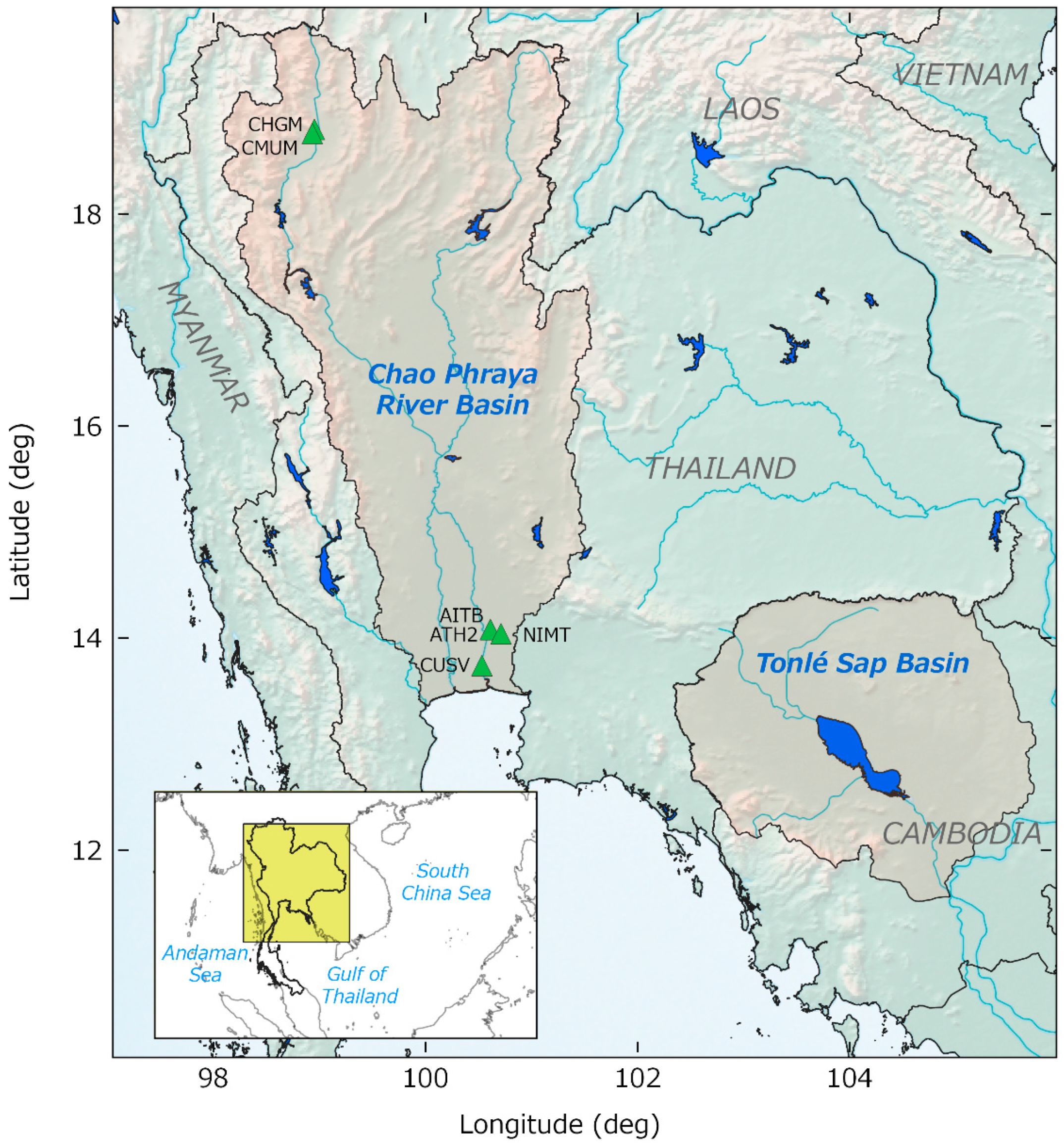
2.1. Study Area
2.2. GRACE Data
2.3. Hydrology Model
2.4. GPS Measurements
2.5. Flood Extent
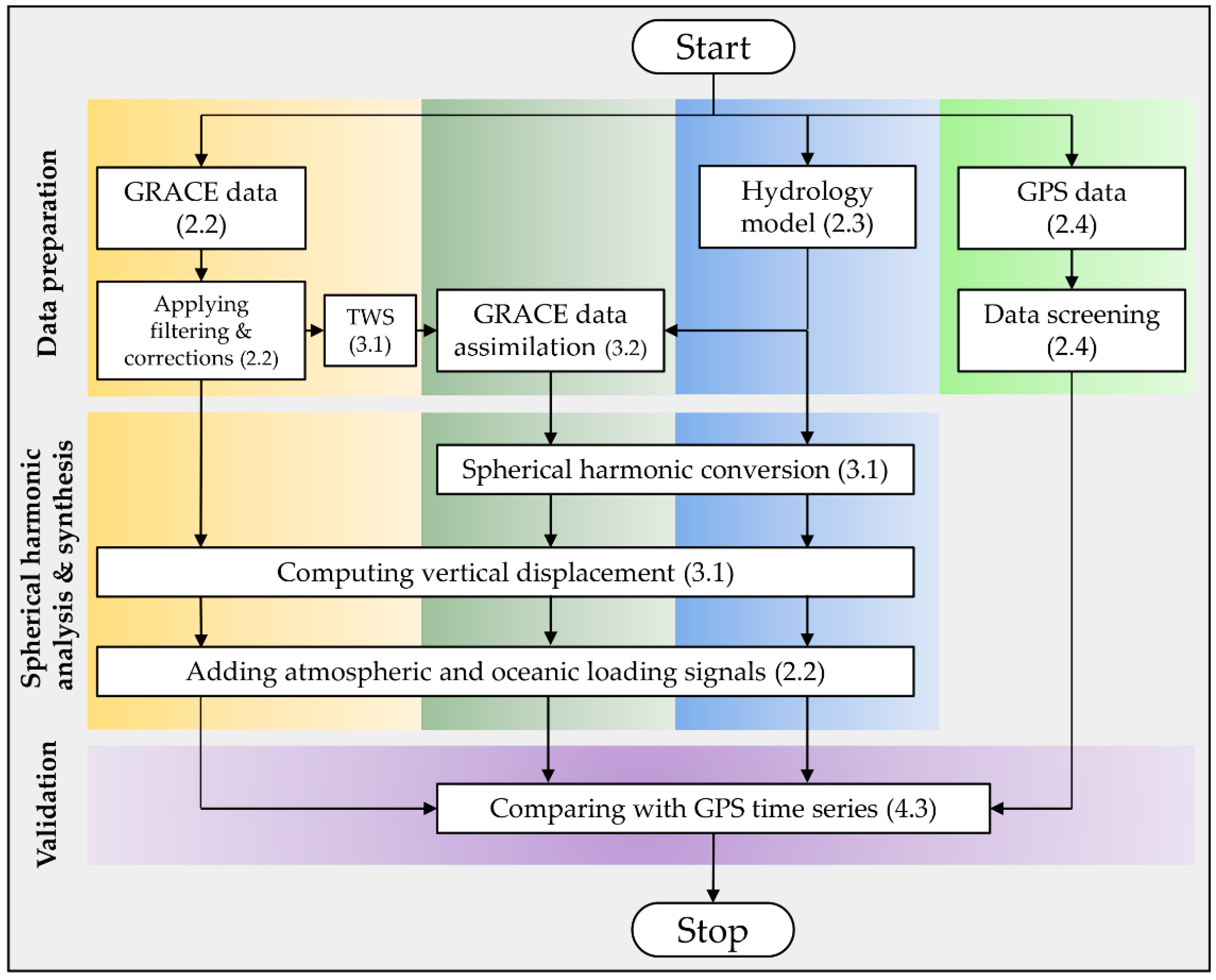
3. Methods
3.1. Computation of Terrestrial Water Storage and Vertical Displacement Variations
3.2. GRACE Data Assimilation
4. Results
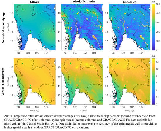
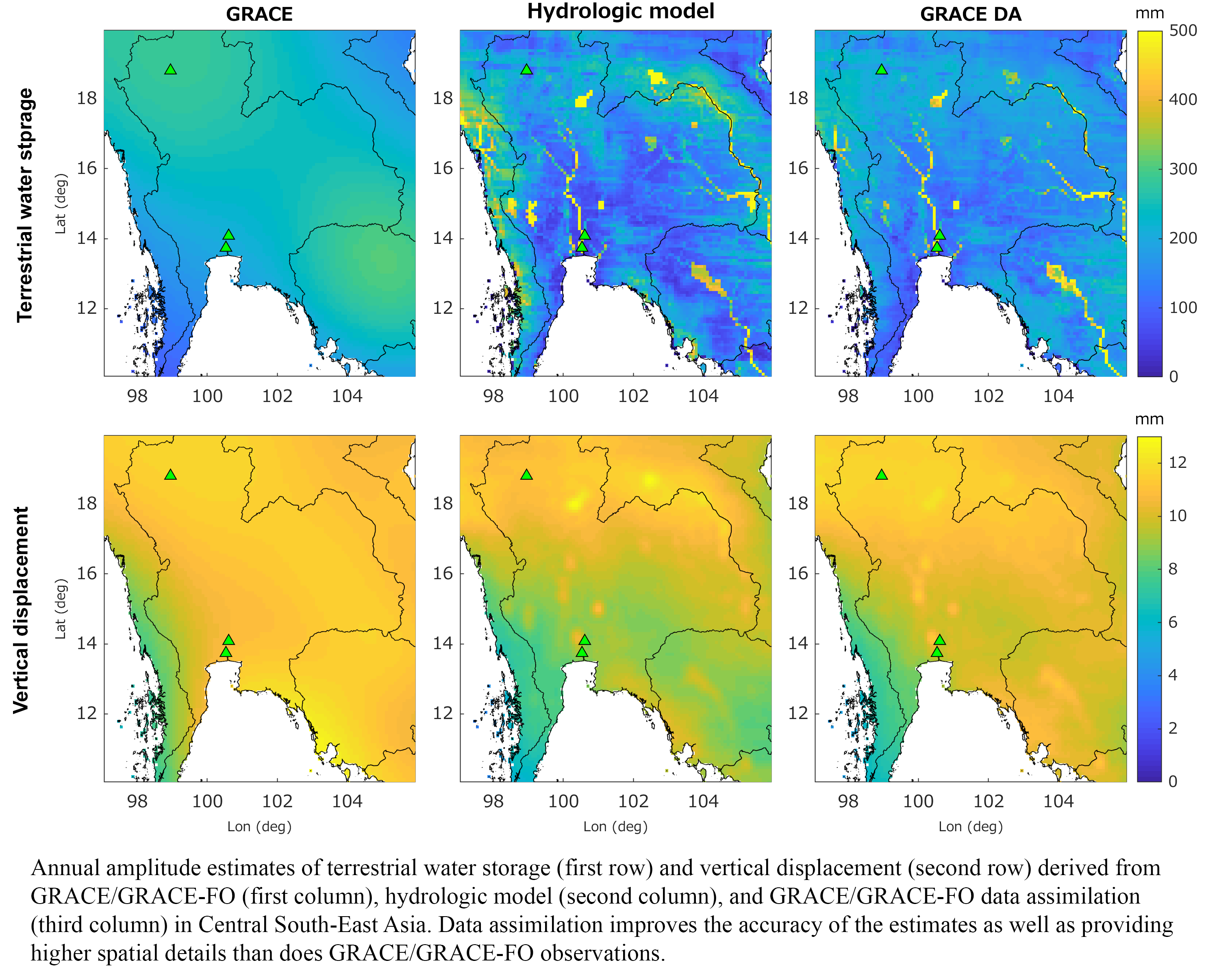
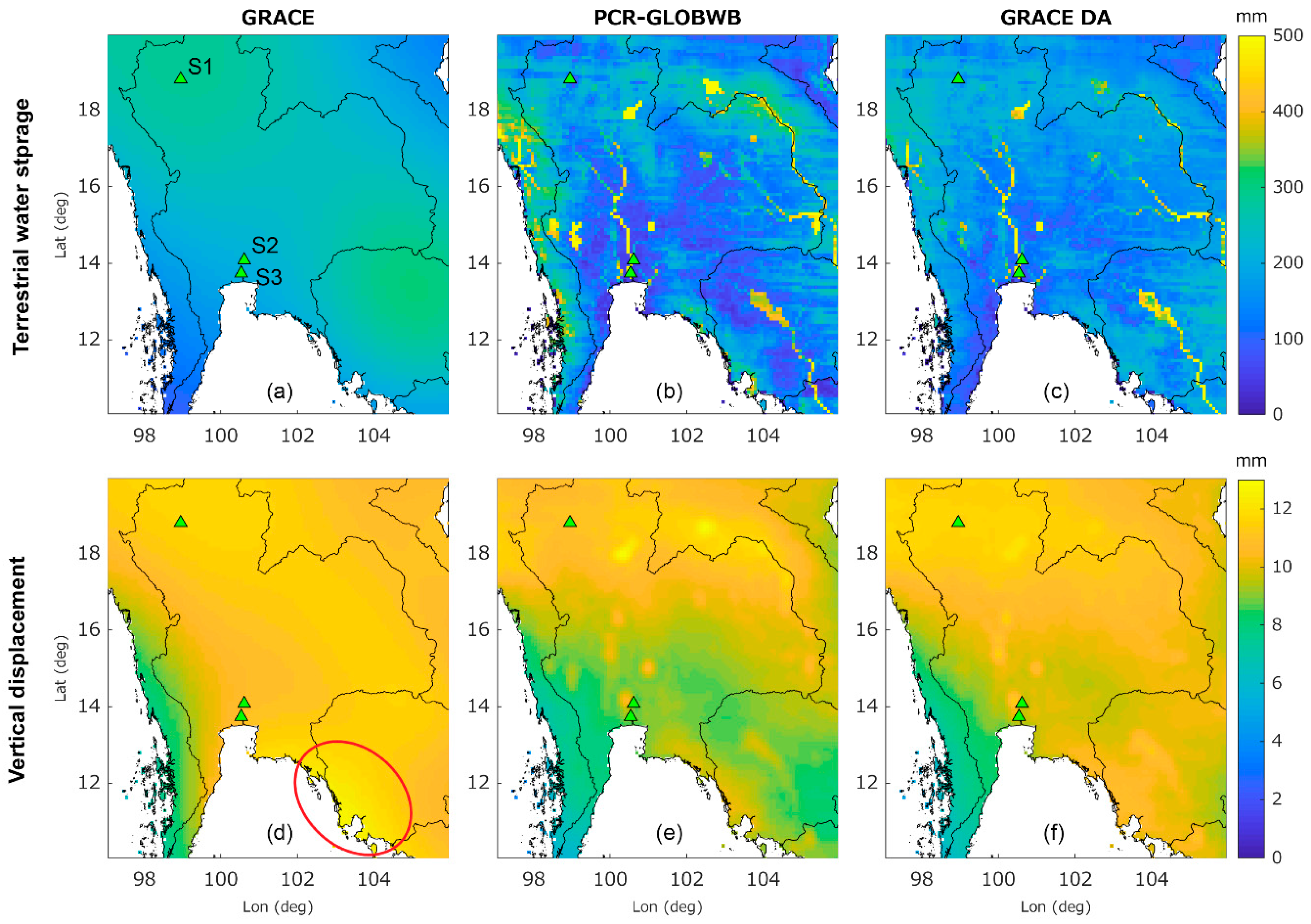
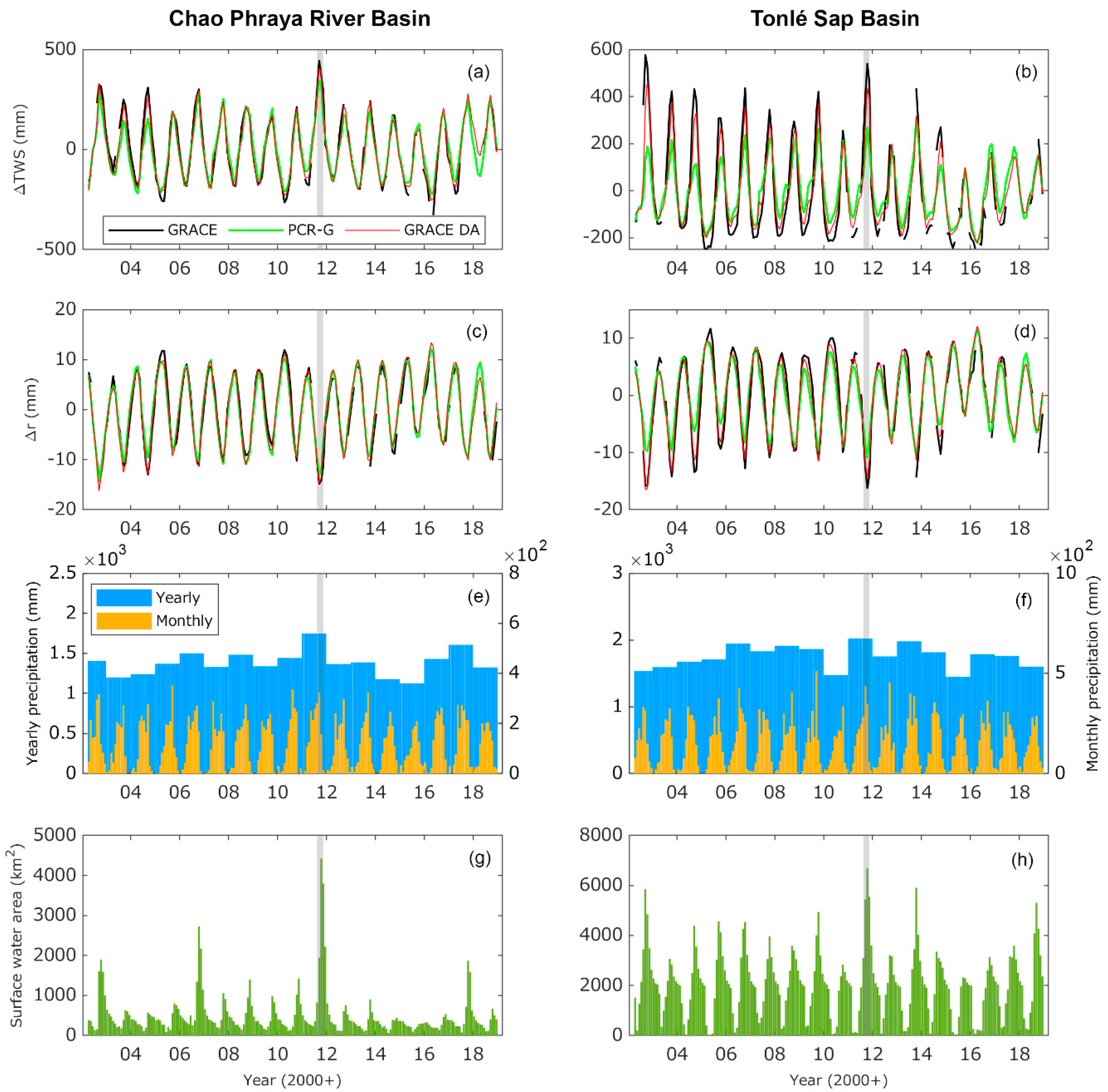
4.1. The Estimations of TWS and Vertical Displacement Variations
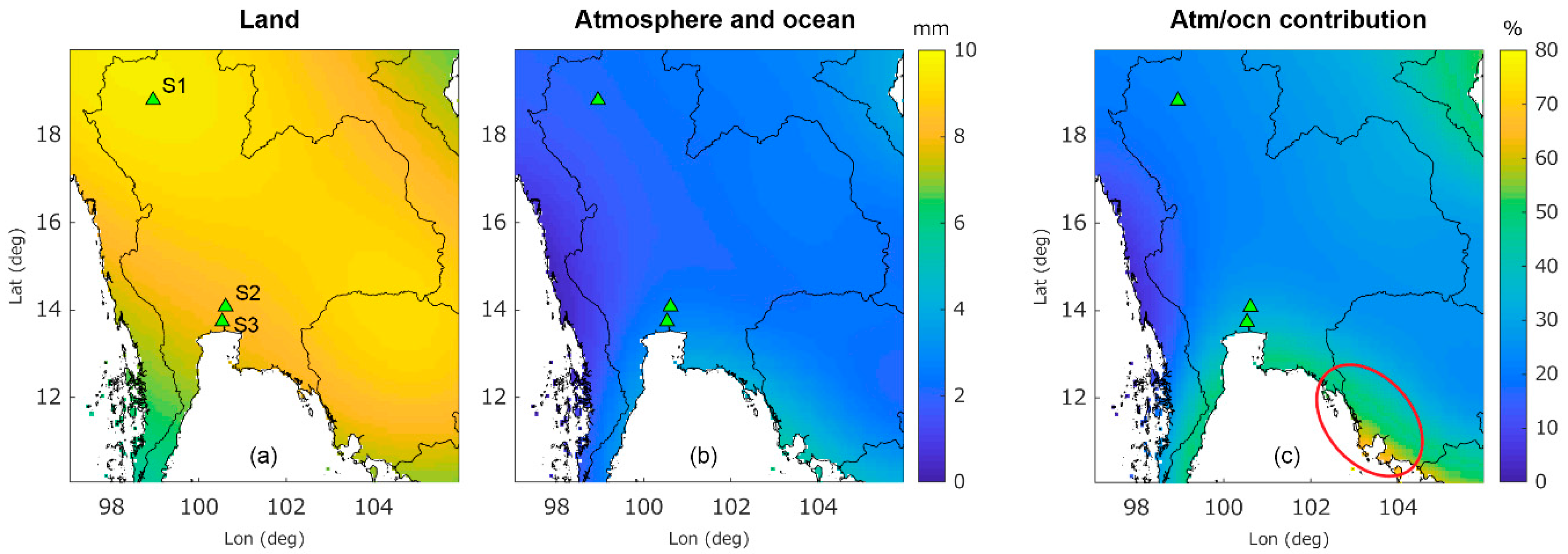
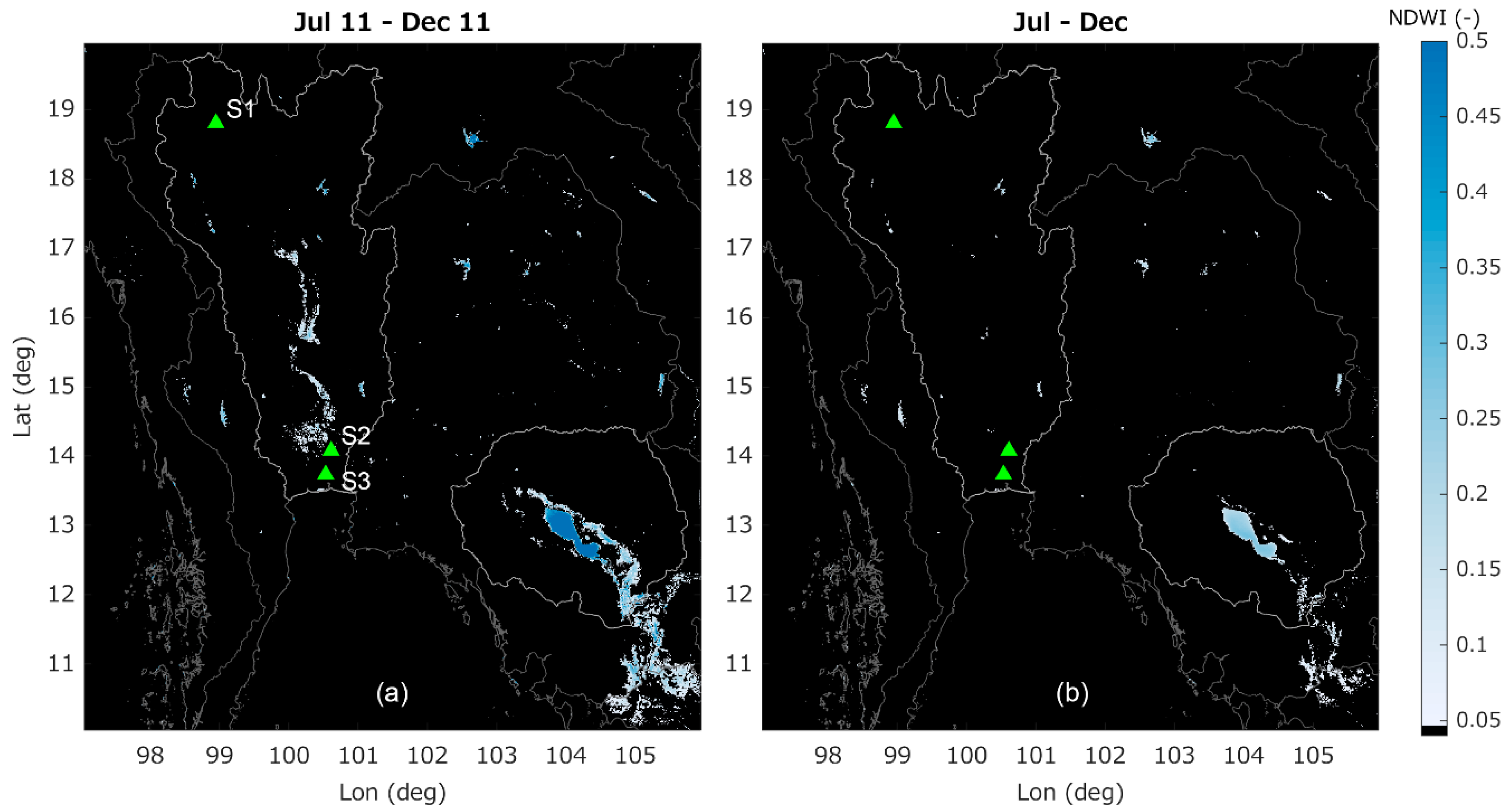
4.2. The Impact of Flooding on Vertical Displacement Estimates
4.3. Validation with GPS Measurements
5. Discussion
6. Conclusions
Author Contributions
Funding
Institutional Review Board Statement
Informed Consent Statement
Data Availability Statement
Acknowledgments
Conflicts of Interest
Appendix A. The Configuration of GRACE Data Assimilation
References
- Tregoning, P.; Watson, C.; Ramillien, G.; McQueen, H.; Zhang, J. Detecting hydrologic deformation using GRACE and GPS. Geophys. Res. Lett. 2009, 36. [Google Scholar] [CrossRef] [Green Version]
- Chaussard, E.; Amelung, F.; Abidin, H.; Hong, S. Sinking cities in Indonesia: ALOS PALSAR detects rapid subsidence due to groundwater and gas extraction. Remote Sens. Environ. 2013, 128, 150–161. [Google Scholar] [CrossRef]
- Phien-Wej, N.; Giao, P.; Nutalaya, P. Land subsidence in Bangkok, Thailand. Eng. Geol. 2006, 82, 187–201. [Google Scholar] [CrossRef]
- Schmidt, D.A.; Burgmann, R. Time-dependent land uplift and subsidence in the Santa Clara valley, California, from a large interferometric synthetic aperture radar data set. J. Geophys. Res. Space Phys. 2003, 108. [Google Scholar] [CrossRef] [Green Version]
- Dill, R.; Dobslaw, H. Numerical simulations of global-scale high-resolution hydrological crustal deformations. J. Geophys. Res. Solid Earth 2013, 118, 5008–5017. [Google Scholar] [CrossRef]
- Fu, Y.; Freymueller, J.T.; Jensen, T. Seasonal hydrological loading in southern Alaska observed by GPS and GRACE. Geophys. Res. Lett. 2012, 39. [Google Scholar] [CrossRef] [Green Version]
- Wang, L.; Chen, C.; Du, J.; Wang, T. Detecting seasonal and long-term vertical displacement in the North China Plain using GRACE and GPS. Hydrol. Earth Syst. Sci. 2017, 21, 2905–2922. [Google Scholar] [CrossRef] [Green Version]
- Heki, K. Seasonal Modulation of Interseismic Strain Buildup in Northeastern Japan Driven by Snow Loads. Science 2001, 293, 89–92. [Google Scholar] [CrossRef] [PubMed]
- Fu, Y.; Argus, D.F.; Landerer, F.W. GPS as an independent measurement to estimate terrestrial water storage variations in Washington and Oregon. J. Geophys. Res. Solid Earth 2015, 120, 552–566. [Google Scholar] [CrossRef]
- Argus, D.F.; Fu, Y.; Landerer, F.W. Seasonal variation in total water storage in California inferred from GPS observations of vertical land motion. Geophys. Res. Lett. 2014, 41, 1971–1980. [Google Scholar] [CrossRef]
- Nahmani, S.; Bock, O.; Bouin, M.-N.; Santamaría-Gómez, A.; Boy, J.-P.; Collilieux, X.; Métivier, L.; Panet, I.; Genthon, P.; De Linage, C.; et al. Hydrological deformation induced by the West African Monsoon: Comparison of GPS, GRACE and loading models. J. Geophys. Res. Space Phys. 2012, 117. [Google Scholar] [CrossRef] [Green Version]
- Fu, Y.; Argus, D.F.; Freymueller, J.T.; Heflin, M.B. Horizontal motion in elastic response to seasonal loading of rain water in the Amazon Basin and monsoon water in Southeast Asia observed by GPS and inferred from GRACE. Geophys. Res. Lett. 2013, 40, 6048–6053. [Google Scholar] [CrossRef]
- Steckler, M.; Nooner, S.L.; Akhter, S.H.; Chowdhury, S.K.; Bettadpur, S.; Seeber, L.; Kogan, M.G. Modeling Earth deformation from monsoonal flooding in Bangladesh using hydrographic, GPS, and Gravity Recovery and Climate Experiment (GRACE) data. J. Geophys. Res. Space Phys. 2010, 115. [Google Scholar] [CrossRef]
- Klein, E.; Duputel, Z.; Zigone, D.; Vigny, C.; Boy, J.-P.; Doubre, C.; Meneses, G. Deep Transient Slow Slip Detected by Survey GPS in the Region of Atacama, Chile. Geophys. Res. Lett. 2018, 45. [Google Scholar] [CrossRef] [PubMed] [Green Version]
- Tregoning, P.; Ramillien, G.; McQueen, H.; Zwartz, D. Glacial isostatic adjustment and nonstationary signals observed by GRACE. J. Geophys. Res. Space Phys. 2009, 114, 114. [Google Scholar] [CrossRef]
- Kouba, J. A Guide to Using International GPS Service (IGS) Products; IGS Central Bureau: Pasadena, CA, USA, 2003. [Google Scholar]
- Saji, A.P.; Sunil, P.; Sreejith, K.M.; Gautam, P.K.; Kumar, K.V.; Ponraj, M.; Amirtharaj, S.; Shaju, R.M.; Begum, S.K.; Reddy, C.D.; et al. Surface Deformation and Influence of Hydrological Mass Over Himalaya and North India Revealed from a Decade of Continuous GPS and GRACE Observations. J. Geophys. Res. Earth Surf. 2020, 125. [Google Scholar] [CrossRef]
- Tapley, B.D.; Bettadpur, S.V.; Ries, J.; Thompson, P.F.; Watkins, M.M. GRACE Measurements of Mass Variability in the Earth System. Science 2004, 305, 503–505. [Google Scholar] [CrossRef] [Green Version]
- Flechtner, F.; Neumayer, K.-H.; Dahle, C.; Dobslaw, H.; Fagiolini, E.; Raimondo, J.-C.; Güntner, A. What Can be Expected from the GRACE-FO Laser Ranging Interferometer for Earth Science Applications? In Remote Sensing and Water Resources; Cazenave, A., Champollion, N., Benveniste, J., Chen, J., Eds.; Springer: Cham, Switzerland, 2016; pp. 263–280. ISBN 978-3-319-32449-4. [Google Scholar]
- Tapley, B.D.; Watkins, M.M.; Flechtner, F.M.; Reigber, C.; Bettadpur, S.; Rodell, M.; Sasgen, I.; Famiglietti, J.S.; Landerer, F.W.; Chambers, D.P.; et al. Contributions of GRACE to understanding climate change. Nat. Clim. Chang. 2019, 9, 358–369. [Google Scholar] [CrossRef]
- Scanlon, B.R.; Zhang, Z.; Save, H.; Wiese, D.N.; Landerer, F.W.; Long, D.; Longuevergne, L.; Chen, J. Global evaluation of new GRACE mascon products for hydrologic applications. Water Resour. Res. 2016, 52, 9412–9429. [Google Scholar] [CrossRef]
- Ahmed, M. Sustainable management scenarios for northern Africa’s fossil aquifer systems. J. Hydrol. 2020, 589, 125196. [Google Scholar] [CrossRef]
- Swenson, S.C.; Lawrence, D.M. Assessing a dry surface layer-based soil resistance parameterization for the Community Land Model using GRACE and FLUXNET-MTE data. J. Geophys. Res. Atmos. 2014, 119. [Google Scholar] [CrossRef]
- King, M.; Moore, P.; Clarke, P.; Lavallée, D. Choice of optimal averaging radii for temporal GRACE gravity solutions, a comparison with GPS and satellite altimetry. Geophys. J. Int. 2006, 166, 1–11. [Google Scholar] [CrossRef] [Green Version]
- Ferreira, V.G.; Montecino, H.D.; Ndehedehe, C.E.; Del Rio, R.A.; Cuevas, A.; De Freitas, S.R.C. Determining seasonal displacements of Earth’s crust in South America using observations from space-borne geodetic sensors and surface-loading models. Earth Planets Space 2019, 71, 84. [Google Scholar] [CrossRef] [Green Version]
- Springer, A.; Karegar, M.A.; Kusche, J.; Keune, J.; Kurtz, W.; Kollet, S. Evidence of daily hydrological loading in GPS time series over Europe. J. Geod. 2019, 93, 2145–2153. [Google Scholar] [CrossRef]
- Tangdamrongsub, N.; Steele-Dunne, S.C.; Gunter, B.C.; Ditmar, P.G.; Weerts, A. Data assimilation of GRACE terrestrial water storage estimates into a regional hydrological model of the Rhine River basin. Hydrol. Earth Syst. Sci. 2015, 19, 2079–2100. [Google Scholar] [CrossRef] [Green Version]
- Scanlon, B.R.; Zhang, Z.; Save, H.; Sun, A.Y.; Schmied, H.M.; Van Beek, L.P.H.; Wiese, D.N.; Wada, Y.; Long, D.; Reedy, R.C.; et al. Global models underestimate large decadal declining and rising water storage trends relative to GRACE satellite data. Proc. Natl. Acad. Sci. USA 2018, 115, E1080–E1089. [Google Scholar] [CrossRef] [Green Version]
- Evensen, G. The Ensemble Kalman Filter: Theoretical formulation and practical implementation. Ocean Dyn. 2003, 53, 343–367. [Google Scholar] [CrossRef]
- Tangdamrongsub, N.; Steele-Dunne, S.C.; Gunter, B.C.; Ditmar, P.G.; Sutanudjaja, E.H.; Sun, Y.; Xia, T.; Wang, Z. Improving estimates of water resources in a semi-arid region by assimilating GRACE data into the PCR-GLOBWB hydrological model. Hydrol. Earth Syst. Sci. 2017, 21, 2053–2074. [Google Scholar] [CrossRef] [Green Version]
- Li, B.; Rodell, M.; Kumar, S.V.; Beaudoing, H.; Getirana, A.; Zaitchik, B.F.; De Goncalves, L.G.; Cossetin, C.; Bhanja, S.N.; Mukherjee, A.; et al. Global GRACE Data Assimilation for Groundwater and Drought Monitoring: Advances and Challenges. Water Resour. Res. 2019, 55, 7564–7586. [Google Scholar] [CrossRef] [Green Version]
- Yin, W.; Han, S.; Zheng, W.; Yeo, I.-Y.; Hu, L.; Tangdamrongsub, N.; Ghobadi-Far, K. Improved water storage estimates within the North China Plain by assimilating GRACE data into the CABLE model. J. Hydrol. 2020, 590, 125348. [Google Scholar] [CrossRef]
- Chanard, K.; Avouac, J.P.; Ramillien, G.; Genrich, J. Modeling deformation induced by seasonal variations of continental water in the Himalaya region: Sensitivity to Earth elastic structure. J. Geophys. Res. Solid Earth 2014, 119, 5097–5113. [Google Scholar] [CrossRef] [Green Version]
- Sutanudjaja, E.H.; Van Beek, L.P.H.; Wanders, N.; Wada, Y.; Bosmans, J.H.C.; Drost, N.; Van Der Ent, R.J.; De Graaf, I.E.M.; Hoch, J.M.; De Jong, K.; et al. PCR-GLOBWB 2: A 5 arcmin global hydrological and water resources model. Geosci. Model Dev. 2018, 11, 2429–2453. [Google Scholar] [CrossRef] [Green Version]
- Van Dam, T.; Wahr, J.M.; Lavallée, D. A comparison of annual vertical crustal displacements from GPS and Gravity Recovery and Climate Experiment (GRACE) over Europe. J. Geophys. Res. Space Phys. 2007, 112. [Google Scholar] [CrossRef] [Green Version]
- Tangdamrongsub, N.; Ditmar, P.; Steele-Dunne, S.; Gunter, B.; Sutanudjaja, E. Assessing total water storage and identifying flood events over Tonlé Sap basin in Cambodia using GRACE and MODIS satellite observations combined with hydrological models. Remote Sens. Environ. 2016, 181, 162–173. [Google Scholar] [CrossRef] [Green Version]
- Jamrussri, S.; Toda, Y. Simulating past severe flood events to evaluate the effectiveness of nonstructural flood countermeasures in the upper Chao Phraya River Basin, Thailand. J. Hydrol. Reg. Stud. 2017, 10, 82–94. [Google Scholar] [CrossRef]
- World Bank. Thai Flood 2011: Rapid Assessment for Resilient Recovery and Reconstruction Planning; World Bank: Washington, DC, USA, 2012. [Google Scholar]
- Swenson, S.; Chambers, D.P.; Wahr, J. Estimating geocenter variations from a combination of GRACE and ocean model output. J. Geophys. Res. Sol. Earth 2008, 113, 08410. [Google Scholar] [CrossRef] [Green Version]
- Loomis, B.D.; Rachlin, K.E.; Wiese, D.N.; Landerer, F.W.; Luthcke, S.B. Replacing GRACE/GRACE-FO With Satellite Laser Ranging: Impacts on Antarctic Ice Sheet Mass Change. Geophys. Res. Lett. 2020, 47. [Google Scholar] [CrossRef]
- Swenson, S.; Wahr, J. Post-processing removal of correlated errors in GRACE data. Geophys. Res. Lett. 2006, 33. [Google Scholar] [CrossRef]
- Jekeli, C. Alternative Methods to Smooth the Earth’s Gravity Field; Scientific Report 327; The Ohio State University: Columbus, OH, USA, 1981. [Google Scholar]
- Caron, L.; Ivins, E.R.; Larour, E.; Adhikari, S.; Nilsson, J.; Blewitt, G. GIA Model Statistics for GRACE Hydrology, Cryosphere, and Ocean Science. Geophys. Res. Lett. 2018, 45, 2203–2212. [Google Scholar] [CrossRef]
- Zhou, H.; Luo, Z.; Tangdamrongsub, N.; Zhou, H.; He, L.; Xu, C.; Li, Q.; Wu, Y. Identifying Flood Events over the Poyang Lake Basin Using Multiple Satellite Remote Sensing Observations, Hydrological Models and In Situ Data. Remote Sens. 2018, 10, 713. [Google Scholar] [CrossRef] [Green Version]
- Dobslaw, H.; Bergmann-Wolf, I.; Dill, R.; Poropat, L.; Thomas, M.; Dahle, C.; Esselborn, S.; König, R.; Flechtner, F. A new high-resolution model of non-tidal atmosphere and ocean mass variability for de-aliasing of satellite gravity observations: AOD1B RL06. Geophys. J. Int. 2017, 211, 263–269. [Google Scholar] [CrossRef] [Green Version]
- Van Beek, L.P.H.; Wada, Y.; Bierkens, M.F.P. Global monthly water stress: 1. Water balance and water availability. Water Resour. Res. 2011, 47. [Google Scholar] [CrossRef]
- Sutanudjaja, E.H.; Van Beek, L.P.H.; De Jong, S.M.; Van Geer, F.C.; Bierkens, M.F.P. Large-scale groundwater modeling using global datasets: A test case for the Rhine-Meuse basin. Hydrol. Earth Syst. Sci. 2011, 15, 2913–2935. [Google Scholar] [CrossRef] [Green Version]
- Sutanudjaja, E.H.; Van Beek, L.P.H.; De Jong, S.M.; Van Geer, F.C.; Bierkens, M.F.P. Calibrating a large-extent high-resolution coupled groundwater-land surface model using soil moisture and discharge data. Water Resour. Res. 2014, 50, 687–705. [Google Scholar] [CrossRef]
- Huffman, G.J.; Bolvin, D.T.; Braithwaite, D.; Hsu, K.; Joyce, R.; Kidd, C.; Nelkin, E.J.; Sorooshian, S.; Tan, J.; Xie, P. NASA Global Precipitation Measurement (GPM) Integrated Multi-SatellitE Retrievals for GPM (IMERG); Algorithm Theoretical Basis Document (ATBD) Version 06; NASAGSFC: Greenbelt, MD, USA, 2019.
- Lu, J.; Sun, G.; McNulty, S.G.; Amatya, D.M. A Comparison of Six Potential Evapotranspiration Methods for Regional Use in the Southeastern United States. JAWRA J. Am. Water Resour. Assoc. 2005, 41, 621–633. [Google Scholar] [CrossRef]
- Blewitt, G.; Hammond, W.C.; Kreemer, C. Harnessing the GPS Data Explosion for Interdisciplinary Science. Available online: https://eos.org/science-updates/harnessing-the-gps-data-explosion-for-interdisciplinary-science (accessed on 30 September 2020).
- Roger, P.J.C.; Vermote, E.F.; Ray, J.P. MODIS Surface Reflectance User’s Guide; Collection 6; NASAGSFC: Greenbelt, MD, USA, 2015.
- McFeeters, S.K. The use of the Normalized Difference Water Index (NDWI) in the delineation of open water features. Int. J. Remote Sens. 1996, 17, 1425–1432. [Google Scholar] [CrossRef]
- Tangdamrongsub, N.; Han, S.-C.; Jasinski, M.F.; Šprlák, M. Quantifying water storage change and land subsidence induced by reservoir impoundment using GRACE, Landsat, and GPS data. Remote Sens. Environ. 2019, 233, 111385. [Google Scholar] [CrossRef]
- Wang, H.; Xiang, L.; Jia, L.; Jiang, L.; Wang, Z.; Hu, B.; Gao, P. Load Love numbers and Green’s functions for elastic Earth models PREM, iasp91, ak135, and modified models with refined crustal structure from Crust 2.0. Comput. Geosci. 2012, 49, 190–199. [Google Scholar] [CrossRef]
- Wahr, J.; Molenaar, M.; Bryan, F. Time variability of the Earth’s gravity field: Hydrological and oceanic effects and their possible detection using GRACE. J. Geophys. Res. Space Phys. 1998, 103, 30205–30229. [Google Scholar] [CrossRef]
- Vishwakarma, B.D.; Devaraju, B.; Sneeuw, N. What Is the Spatial Resolution of grace Satellite Products for Hydrology? Remote Sens. 2018, 10, 852. [Google Scholar] [CrossRef] [Green Version]
- Wouters, B.; Chambers, D.P. Analysis of seasonal ocean bottom pressure variability in the Gulf of Thailand from GRACE. Glob. Planet. Chang. 2010, 74, 76–81. [Google Scholar] [CrossRef]
- Sharma, A.; Wasko, C.; Lettenmaier, D.P. If Precipitation Extremes Are Increasing, Why Aren’t Floods? Water Resour. Res. 2018, 54, 8545–8551. [Google Scholar] [CrossRef]
- Ferreira, V.G.; Liu, Z.; Montecino, H.C.; Yuan, P.; Kelly, C.I.; Mohammed, A.S.; Han, L.Y. Reciprocal comparison of geodetically sensed and modeled vertical hydrological loading products. Acta Geod. Geophys. 2019, 55, 23–49. [Google Scholar] [CrossRef]
- Wahr, J.M.; Swenson, S.; Velicogna, I. Accuracy of GRACE mass estimates. Geophys. Res. Lett. 2006, 33. [Google Scholar] [CrossRef] [Green Version]
- Bettinelli, P.; Avouac, J.; Flouzat, M.; Bollinger, L.; Ramillien, G.; Rajaure, S.; Sapkota, S. Seasonal variations of seismicity and geodetic strain in the Himalaya induced by surface hydrology. Earth Planet. Sci. Lett. 2008, 266, 332–344. [Google Scholar] [CrossRef]
- Van Dam, T.; Collilieux, X.; Wuite, J.; Altamimi, Z.; Ray, J.R. Nontidal ocean loading: Amplitudes and potential effects in GPS height time series. J. Geod. 2012, 86, 1043–1057. [Google Scholar] [CrossRef] [Green Version]
- Mémin, A.; Boy, J.-P.; Santamaría-Gómez, A. Correcting GPS measurements for non-tidal loading. GPS Solut. 2020, 24, 45. [Google Scholar] [CrossRef]


| Evaluation Sites | GPS Sites | Data Periods | Latitude (deg) | Longitude (deg) |
|---|---|---|---|---|
| S1 | CHGM | 2010–2012 | 18.803 | 98.950 |
| CMUM * | 2014–2018 | 18.761 | 98.932 | |
| S2 | AITB | 2010–2014 | 14.079 | 100.612 |
| ATH2 | 2014–2017 | 14.082 | 100.613 | |
| NIMT | 2005–2014 | 14.043 | 100.714 | |
| S3 | CUSV * | 2008–2018 | 13.736 | 100.534 |
| ΔTWS | Δr | |||||
|---|---|---|---|---|---|---|
| Amp (mm) | ρ (-) | RMSD (mm) | Amp (mm) | ρ (-) | RMSD (mm) | |
| The Chao Phraya River Basin | ||||||
| GRACE | 197.35 | - | - | 9.16 | - | - |
| PCR-GLOBWB | 171.76 | 0.96 | 50.93 | 7.70 | 0.89 | 115.63 |
| GRACE DA | 187.84 | 0.99 (3%) | 29.76 (42%) | 8.71 | 0.97 (9%) | 64.41 (44%) |
| The Tonlé Sap basin | ||||||
| GRACE | 236.51 | - | - | 8.07 | - | - |
| PCR-GLOBWB | 139.15 | 0.89 | 3.99 | 6.89 | 0.86 | 3.33 |
| GRACE DA | 185.51 | 0.93 (4%) | 2.82 (29%) | 7.78 | 0.93 (8%) | 2.51 (25%) |
| Amplitude (mm) | Phase (month) | |||||||
|---|---|---|---|---|---|---|---|---|
| S1 | S2 | S3 | Avg | S1 | S2 | S3 | Avg | |
| GPS | 10.26 | 7.37 | 8.39 | 8.67 | 4.23 | 4.60 | 4.57 | 4.47 |
| GRACE | 10.00 | 8.63 | 8.71 | 9.11 | 4.15 | 4.54 | 4.54 | 4.41 |
| PCR-GLOBWB | 9.23 | 6.72 | 6.96 | 7.64 | 4.06 | 4.19 | 4.07 | 4.11 |
| GRACE DA | 9.83 | 7.51 | 7.56 | 8.30 | 4.11 | 4.22 | 4.11 | 4.15 |
| ρ (-) | RMSD (mm) | RMS Reduction (%) | ||||||||||
|---|---|---|---|---|---|---|---|---|---|---|---|---|
| S1 | S2 | S3 | Avg | S1 | S2 | S3 | Avg | S1 | S2 | S3 | Avg | |
| Including atmospheric and oceanic signals | ||||||||||||
| GRACE | 0.77 | 0.78 | 0.89 | 0.81 | 5.70 | 4.57 | 3.60 | 4.62 | 39.33 | 36.70 | 53.44 | 43.16 |
| PCR-GLOBWB | 0.75 | 0.75 | 0.84 | 0.78 | 5.86 | 4.77 | 4.26 | 4.96 | 36.56 | 33.11 | 44.16 | 37.94 |
| GRACE DA | 0.77 | 0.77 | 0.86 | 0.80 | 5.76 | 4.64 | 4.06 | 4.82 | 37.33 | 34.78 | 49.97 | 40.69 |
| Excluding atmospheric and oceanic signals | ||||||||||||
| GRACE | 0.72 | 0.72 | 0.85 | 0.76 | 6.30 | 4.98 | 4.11 | 5.13 | 30.83 | 28.92 | 46.79 | 35.51 |
| PCR-GLOBWB | 0.72 | 0.66 | 0.74 | 0.71 | 6.33 | 5.29 | 4.93 | 5.52 | 29.62 | 22.08 | 32.63 | 28.11 |
| GRACE DA | 0.74 | 0.67 | 0.77 | 0.73 | 6.22 | 5.19 | 4.67 | 5.36 | 32.02 | 24.56 | 34.91 | 30.50 |
Publisher’s Note: MDPI stays neutral with regard to jurisdictional claims in published maps and institutional affiliations. |
© 2021 by the authors. Licensee MDPI, Basel, Switzerland. This article is an open access article distributed under the terms and conditions of the Creative Commons Attribution (CC BY) license (http://creativecommons.org/licenses/by/4.0/).
Share and Cite
Tangdamrongsub, N.; Šprlák, M. The Assessment of Hydrologic- and Flood-Induced Land Deformation in Data-Sparse Regions Using GRACE/GRACE-FO Data Assimilation. Remote Sens. 2021, 13, 235. https://0-doi-org.brum.beds.ac.uk/10.3390/rs13020235
Tangdamrongsub N, Šprlák M. The Assessment of Hydrologic- and Flood-Induced Land Deformation in Data-Sparse Regions Using GRACE/GRACE-FO Data Assimilation. Remote Sensing. 2021; 13(2):235. https://0-doi-org.brum.beds.ac.uk/10.3390/rs13020235
Chicago/Turabian StyleTangdamrongsub, Natthachet, and Michal Šprlák. 2021. "The Assessment of Hydrologic- and Flood-Induced Land Deformation in Data-Sparse Regions Using GRACE/GRACE-FO Data Assimilation" Remote Sensing 13, no. 2: 235. https://0-doi-org.brum.beds.ac.uk/10.3390/rs13020235