Article

Effects of the COVID-19 Lockdown on Urban Light Emissions: Ground and Satellite Comparison

by
Máximo Bustamante-Calabria
1,*,
Alejandro Sánchez de Miguel
1,2,3,
Susana Martín-Ruiz
1,
Jose-Luis Ortiz
1,
José M. Vílchez
1,
Alicia Pelegrina
1,
Antonio García
1,
Jaime Zamorano
3,
Jonathan Bennie
4 and
Kevin J. Gaston
2
1
Instituto de Astrofísica de Andalucía, Glorieta de la Astronomía, s/n, 18008 Granada, Spain
2
Environment and Sustainability Institute, University of Exeter, Penryn, Cornwall TR10 9FE, UK
3
Departamento de Física de la Tierra y Astrofísica, Instituto de Física de Partículas y del COSMOS (IPARCOS), Universidad Complutense, 28040 Madrid, Spain
4
Centre for Geography and Environmental Science, University of Exeter, Penryn, Cornwall TR10 9FE, UK
*
Author to whom correspondence should be addressed.
Submission received: 20 November 2020 / Revised: 21 December 2020 / Accepted: 10 January 2021 / Published: 13 January 2021
(This article belongs to the Special Issue Light Pollution Monitoring Using Remote Sensing Data)

Abstract

:
‘Lockdown’ periods in response to COVID-19 have provided a unique opportunity to study the impacts of economic activity on environmental pollution (e.g., NO2, aerosols, noise, light). The effects on NO2 and aerosols have been very noticeable and readily demonstrated, but that on light pollution has proven challenging to determine. The main reason for this difficulty is that the primary source of nighttime satellite imagery of the earth is the SNPP-VIIRS/DNB instrument, which acquires data late at night after most human nocturnal activity has already occurred and much associated lighting has been turned off. Here, to analyze the effect of lockdown on urban light emissions, we use ground and satellite data for Granada, Spain, during the COVID-19 induced confinement of the city’s population from 14 March until 31 May 2020. We find a clear decrease in light pollution due both to a decrease in light emissions from the city and to a decrease in anthropogenic aerosol content in the atmosphere which resulted in less light being scattered. A clear correlation between the abundance of PM10 particles and sky brightness is observed, such that the more polluted the atmosphere the brighter the urban night sky. An empirical expression is determined that relates PM10 particle abundance and sky brightness at three different wavelength bands.

Graphical Abstract

1. Introduction

The COVID-19 pandemic has caused dramatic changes in human habits and activities across much of the world. This has been especially true during so-called ’lockdown’ periods, when the local, regional or national activities and movements of people have been markedly curtailed to reduce rates and levels of viral transmission. The details of these restrictions, and the extent and vigour with which they have been enforced, have varied greatly between different countries. Nonetheless, these unusual situations have acted as valuable ’natural experiments’, allowing novel analyses to be conducted of the relationships between levels of human activity and levels of change to the environment, by comparing important potential impacts prior to and during lockdown periods. For example, this has been done for NO2 concentrations in urban areas and globally for aerosol content [1,2], noise [3], and seismic tremors [4].
Many of the environmental impacts of human activity, and hence the effects of the lockdown periods, can be monitored remotely through satellites. However, perhaps surprisingly, this has proven challenging to do at large regional or global scales for nighttime light emissions, which have been recognised as both a valuable indicator of human population density, urbanisation and economic activity [5,6], and also as themselves having important impacts on human health and the natural environment [7,8,9,10]. The primary source of remote sensing data on nighttime light emissions is the Suomi-North Polar Partnership/Visible Infrared Imaging Radiometer Suite-DayNightBand (SNPP/VIIRS-DNB). This provides data of intermediate spatial resolution using a panchromatic sensor, but its observation time is after 01:30 local time limiting its usefulness for determining changes in nighttime lighting at times when people are predominantly active. Sensors are also carried on other satellite platforms, but variously have limited spatial coverage, require substantial data calibration, and/or are private and with data costs that are prohibitive for monitoring for research purposes [11]. Images of the earth taken by astronauts aboard the International Space Station (ISS) using DSLR cameras are also available [12], have high resolution and are multi-spectral, but are not systematically acquired in space or time, also greatly limiting their suitability.
Accepting these limitations on a broad scale places disproportionate significance on ground-based measurements of changes in artificial nighttime lighting as a means of determining the effects of COVID-19 lockdown periods. Unfortunately, the availability of such data is quite limited, although there are ongoing attempts both to build and maintain networks of monitoring sensors [13,14] and to provide platforms to encourage and collate regular spot measurements by citizen scientists [15].
Here we determine the impacts of a COVID-19 lockdown on artificial nighttime light emissions for an exemplar, the city of Granada, Spain, using both satellite and ground-based measurements. In Spain the general lockdown, which started on 14 March 2020, was particularly severe to counteract a steep rate of spread of the infection. Since 14 March Spain started one of the most strict lockdowns of the Europe, shutting down of school and university classes and trips outside home. Since the 30 March, all businesses and companies should close except for the essential services. Restrictions were not fully lifted until mid June. As an example, the Alhambra palace, the main touristic attraction of the city, was not reopened until June 17th.

2. Methods

2.1. Satellite Data

For satellite images of Granada we used the SNPP-VIIRS/DNB VNP46A1 product [16]. Details on the image processing undertaken are provided in Román et al. (2018) [16], but briefly, images were corrected for atmospheric, topographic and cloud effects. Radiometric calibration was carried out but seasonal and moon effects were not taken into account. Therefore, for this paper, images with no moon illumination were selected, considering only those taken two days prior or two days after the new moon, and only images obtained in January to May were used. Only 27 images in total fulfilled these selection criteria: 5 images for 2018, 7 images for 2019 and 14 images for 2020. Of this last group, 6 images were obtained before the lockdown and 8 during the lockdown. In some months, such as April, only two images were available, due to cloud cover [17]. The images were manually inspected to detect any kind of cloud or fog features (blurriness) or anomalous dimming that could be explained by image acquisition at very shallow angles. The photometry was performed using “FunTools” [18] and the visualization was done with SAO-DS9 [19]. The flux of a 10 × 10 km area has been averaged. The median values per month have been calculated as reference. As central value has been considered the ratio between the median values prior to lockdown and during lockdown. As lowest value has been considered the lowest highest emission during the lockdown divided by the lowest emission prior to lockdown; highest value corresponds to lowest emission during the lockdown divided by the highest emission prior to lockdown.

2.2. Ground-Based Sky Brightness Measurements

In order to measure sky brightness from the ground we used a set of Sky Quality Meters (SQM) [20,21]. The SQM measures night sky brightness and has been used in a large number of studies directly or indirectly concerned with light pollution [22,23,24]. It has a spectral response from 320–700 nm, approximately overlapping the Johnson B and V bands used in astronomical photometry. We used the SQM-LE model, a lensed version with Ethernet connection whose lens reduces the angular sensitivity to ∼20 (full width at half maximum, FWHM) around the zenith. The SQM photometers directly provide data in magnitudes per square arcsecond (magSQM/arcsec2) with a systematic error of 10 per cent (0.1 mag/arcsec2) according to the manufacturer [25]. Note that the mag/arcsec2 scale used in astronomy is somewhat counter-intuitive for people outside the field because it is logarithmic, and because the brighter the sky the smaller the value (for more information on its equivalence with other units, see Bará et al. (2020) [26] and Sánchez de Miguel et al. (2017) [24]).
The set of SQM devices consists of three units situated on the roof of the Instituto de Astrofísica de Andalucía-CSIC (IAA-CSIC) (lat = N 37.1616 , long = W 3.59036 , h = 685 m above mean sea level) located inside the city of Granada. Two of them are equipped with specific B and V Johnson band filters, whereas the third one is used without any added filter. All devices are weatherproof to protect them from outdoor conditions. The material used for the windows of the weatherproof is made of soda-lime glass, and therefore, the devices have been corrected subtracting 0.11 mag/arcsec2 from all readings. Each SQM sends data through the internet to a Raspberry Pi unit for storage and time-tagging and made about 1000 recordings of sky brightness over a night. We use the open-source software PySQM [27] for these operations.
In addition, the Sierra Nevada Observatory (OSN), located more than 2000 m above and more than 20 km away from the city of Granada (lat = N 37.0642 , long = W 3.38472 , h = 2900 mamsl), is equipped with an All-Sky Transmission MONitor (ASTMON), an imaging device that measures sky brightness in the UBVRI Johnson bands at all-sky locations [28], not just at the zenith. The instrument is fully robotic, i.e., it performs all astronomical data reduction and calibration tasks automatically, obtaining maps of sky brightness through the night. For this study, we selected the values of sky brightness at an azimuth and altitude where the glow of Granada’s city is clearly observed (∼20 above the horizon) as shown in Figure 1. This point was carefully chosen to avoid saturated values caused by its proximity to the city. Locations are shown in the Figure 2.
The SQM sensors equipped with V and B Johnson filters were cross calibrated using the ASTMON device for their respective bands using the values at the zenith position. As Cinzano (2005) [20] showed, the SQM with V and B Johnson filters are very good match to the pure V Johnson and B Johnson filters astronomical filters. So, the calibration error 0.1 mag/arcsec2 is mainly for the SQM without added filter and not for the cross calibrated ones, that probably can achieve better performance.
We analyzed data from January, February and until 14 March 2020 to represent the conditions prior to the lockdown, and data from 14 March until 23 May to represent the lockdown conditions. Sky brightness data are extremely sensitive to cloud cover and lunar phase. In astronomy, sky brightness measurements are reported only for moonless nights and for completely cloudless nights. For this study, we did the same. Cloudless nights were selected following the criterion that there was no flickering in the measurements with a standard deviation of 0.1 mag/arcsec2. Sky brightness is usually measured at the zenith. Unfortunately, not all of the measurements reported in the literature specify whether these are of the sky background (removing the stellar contribution) or of the night sky containing stars. SQM devices do not correct for starlight contribution. The stellar contribution might seem negligible but it is not, at least for regions with little light pollution, and this is especially relevant when the Milky Way or other dense stellar regions fall within the viewing cone of SQM. To estimate this seasonal effect from our measurements, we analyzed SQM data from our remote observatory at La Sagra (lat = N 37.98 , long = W 2.56 , h = 1530 mamsl) which has minimal light pollution in order to determine the amount of change from the period of January-February to the lockdown period. We used data for 3 years to have a robust estimation that would not be affected by weather conditions. See Appendix A.

2.3. Pollution Data

Atmospheric pollution data were obtained from the measuring station of the Granada Congress Palace, published by the Junta de Andalucía and available on the Granada City Council website [29]. This station is the nearest to the IAA headquarters (coord. UTM: X = 446,721, Y = 4,113,421). We focused on the concentration of PM10 particles (particles with diameter <10 μm) and nitrogen dioxide, two pollutants directly related to vehicle emissions and therefore to urban activity. The concentration values (μg/m3) were obtained every hour, so in order to study possible correlations with the brightness of the sky, we selected the measurements of the SQM devices installed in the IAA-CSIC. Similarly we have taken measurements with the ASTMON of the OSN (at a point approximately 20° above the city of Granada) with different filters. All data correspond to valid nights and coinciding in time with the measurements of the concentration of particles and nitrogen dioxide. Thus we gathered a sample of 137 measurements in the night hours distributed from January to May 2020.

2.4. Ground Inspections

Special permit was requested to document the qualitative light atmosphere of the city of Granada at night. We were able to record several geolocated videos and one time-lapse of the turn off of the Alhambra palace. The inspection results indicated that, as expected, all non essential economic activities were stopped but, more important, that most of commercial lighting was off with few exceptions, like the Nevada commercial centre that was fully lighted all night long as usual. The monuments and street lighting apparently were at their usual turn off times. On Figure 3 can be seen jumps that correspond to the turn off of some of the monuments and street lighting. For example, at 00:00 the highway reduces its intensity to 1/3 of the nominal by turning off 2/3 of the street lights. The jump of the 2:00 corresponds to the turn off of the Alhambra palace and other monuments. Most of the lights that are usually on all night were still on during the lockdown (with the exception of hotels and some shops, like the Barceló Granada Congress hotel, that usually is all night on, but was turned off during the inspections). During the inspection performed between 2:00 until 6:00, only 3 pedestrians were reported on a city with very active night live in normal circumstances. These inspections where performed 8 May and 7 May respectively.

3. Results

3.1. Satellite Data

Figure 4 shows a comparison of satellite imagery of Granada on clear and moonless nights prior to lockdown and during lockdown. Quantitative analysis indicates that the average intensity of emissions decreased by around 5 13 + 5 % during the lockdown. Comparison of 2018 and 2019 data indicate similar emissions values, although Granada has an ongoing municipal program of transition from High Pressure Sodium (HPS) to LED lighting, so this can only be considered as a lower threshold of change. The dispersion of the day to day intensity observations is of 14%, although it is worth mentioning that the lowest values of the series occurred during the lockdown. The brightest individual light source in Granada (indicated as “Nevada” in the figure), which was lit up constantly during the lockdown is not visible on many of the images because of the angle of observation. This illustrates the important role of the angle of observations in these measurements. Some other research has not consider this potential issue [30,31,32].

3.2. Ground-Based Data

3.2.1. Measurements Comparing Two Time Intervals on Different Nights

As a first approach to analysing the SQM data, values were compared for two time intervals, one before midnight (from 21:00 to 22:00 UT) and another one after midnight (from 2:00 to 3:00 UT). This has been done to see if the changes in lighting and those associated with the decrease in activity are reflected in any way in the values of sky brightness in different filters, taking into account that part of the ornamental lighting is turned off in the second half of the night and that the intensity of the general lighting decreases after legal midnight. 
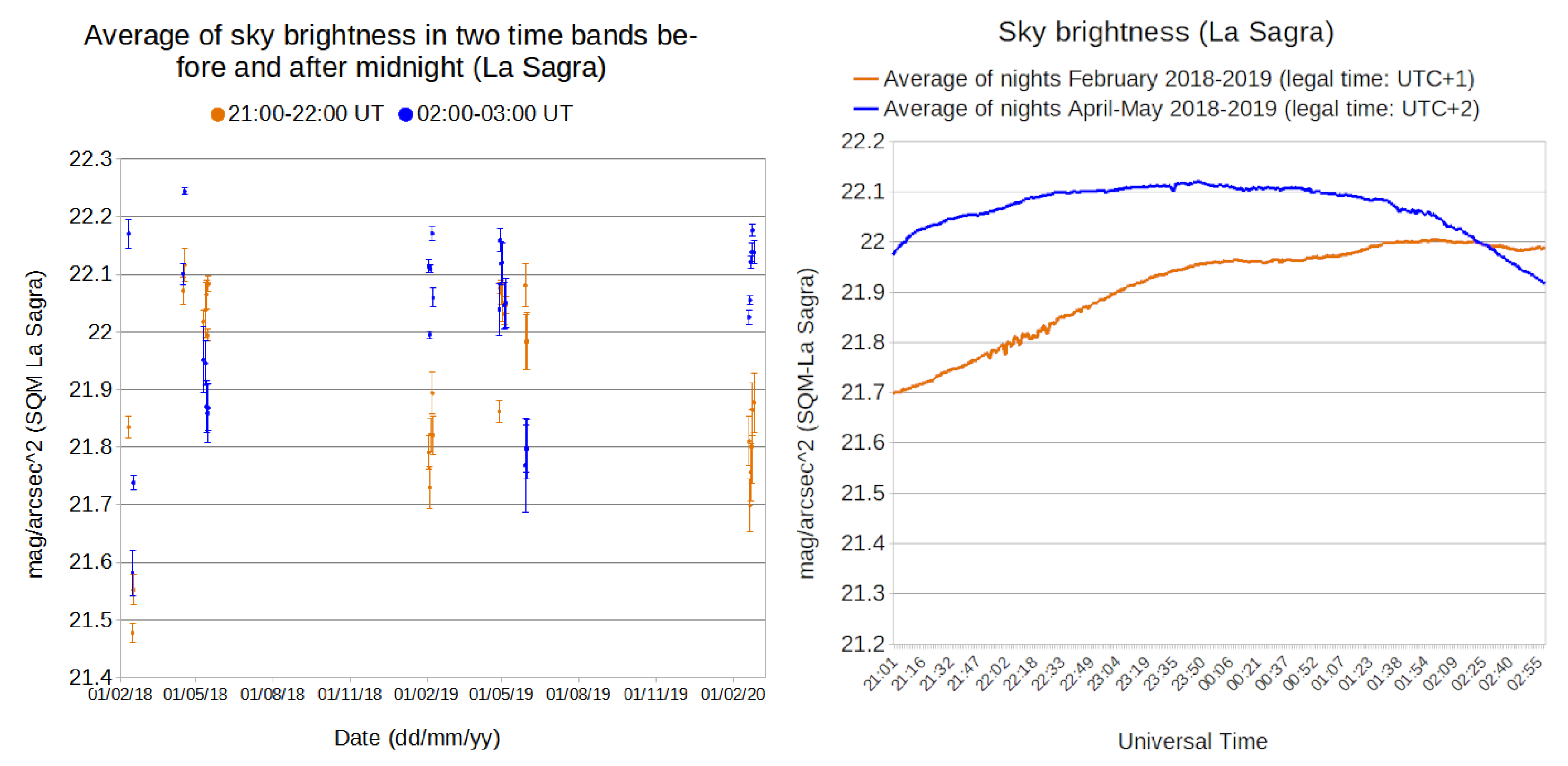
Figure 5 shows the average values of sky brightness from the IAA headquarters in the two time intervals mentioned and at the valid nights, and the average of the B-V colour index which results from subtracting the measurements obtained with the two filters in these time intervals.
We have defined two groups of data based on the pandemic’s policies in Spain: from the days of 26 January and 19–26 February; and from the days of 15, 22, 23, 28, 29, 30 April and 17–22 May. The first group corresponds to pre-lockdown sky brightness and the second to sky brightness obtained at the time of lockdown. The first thing to note is that both in the brightness measurement and in the B-V index there is a clear difference between the first hours of the night and the last hours, especially before lockdown: from 21:00 to 22:00 UT the night sky of Granada is on average 0.54 mag/arcsec2 brighter than from 2:00 to 3:00 UT. Similarly, the average value of B-V is higher from 2:00 to 3:00 UT (B-V is 1.28 after midnight and 1.11 before midnight, so a 0.17 difference).
The variation in the colour index suggests that this is a consequence of the turning off of ornamental lighting (examples are the Alhambra Palace illumination and facade illuminations of several monuments) and private lighting (aka. cars, private outdoor lighting, commercial lighting and indoor lighting), as most of the lamps used for ornamental lighting and private outdoor lighting are metal halide lamps, or have been replaced by LED that produce white or blue-white light with a significant emission in blue, so that once they are switched off the records of the photometer with B filter are significantly higher due to the lower brightness in this band (see Figure 6). This effect has been documented before in many other cities, like Berlin or Madrid [33,34,35].
This difference between night hours also occurred during the lockdown, although to a lesser extent. During lockdown, the Granada sky between 21:00 and 22:00 UT was on average 0.24 mag/arcsec2 brighter than 2:00 to 3:00 UT, while in the B-V index there was a difference of 0.12.
If we compare the days before and during the lockdown, the Granada sky between 21:00 and 22:00 UT was 0.34 mag/arcsec2 darker after its declaration; the difference was 0.04 mag/arcsec2 from 3:00 to 4:00. For the B-V index the differences were greater in the first half of the night (0.17) than in the early morning hours (0.12).

3.2.2. Evolution of Measurements during the Night. Average Nights before and during Lockdown

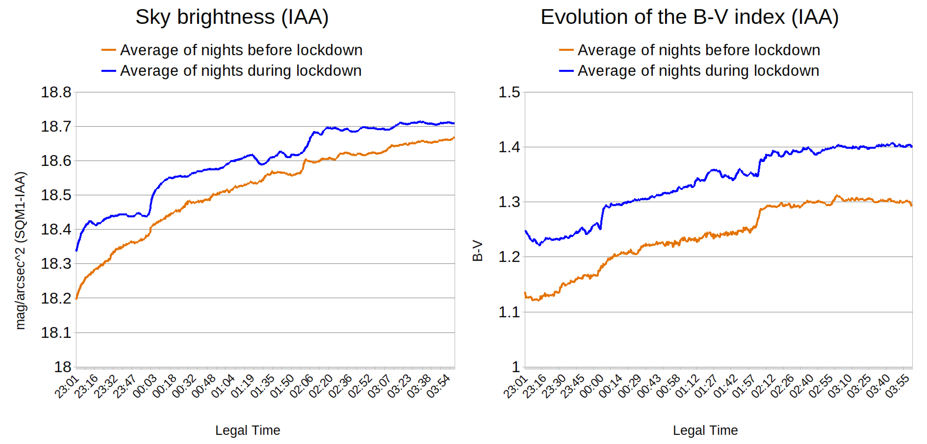
Instead of analysing the average values in time periods before and after midnight, the average variation between 23:00 and 4:00 (legal time: UTC+1) of the brightness of the Granada sky and its colour index can be compared between February and April and May (legal time UTC+2). The average curve for the last week of February (Figure 3, left brown line) represents a more or less progressive darkening over the course of the night from 18.2 mag/arcsec2 to over 18.6 at 4:00, with a steeper slope until midnight and then smoothing out. There are three steps or “jumps” in the curve: the first (and greatest) occurs at about 23:00; the second occurs at 00:00 (midnight legal time) and is less noticeable than the other two; and the third one occurs at 2:00. If we look at the B-V curve (Figure 3, right brown line), the 2:00 step appears while the others are not so clear. It also appears on the curve for the days following the lockdown (blue line, summer time: UTC+2). We can infer that at that time some important lighting with a considerable emission in the blue band is switched off. The other steps may be related to a decrease in the intensity of public lighting, and in B-V a slight increasing can also be seen at midnight. We can interpret this as a spectral power distribution slanting more toward long wavelengths (i.e., blue light is being removed from the zenith).
The curves for the days following the lockdown (blue lines) show a greater divergence from the previous period in the early hours of the night, with higher values both in darkness (between 18.4 and 18.6 mag/arcsec2) and in B-V (close to 1.3). In this case the legal midnight step is much more pronounced. If this is due to a decrease in the intensity of street lighting, it is interesting that before the lockdown this was not so clearly seen. The behaviour of the B-V graph can give some clues: before the lockdown it starts from values between 1.1 and 1.2 without exceeding 1.2 until after midnight, while in April it stays close to 1.3 until it reaches 1.4 in the second half of the night. In the first case, there is a greater brightness in filter B, which also decreases progressively as the night progresses, producing only a jump of some importance at 2:00.

3.2.3. Evolution of Air Pollution and Sky Brightness

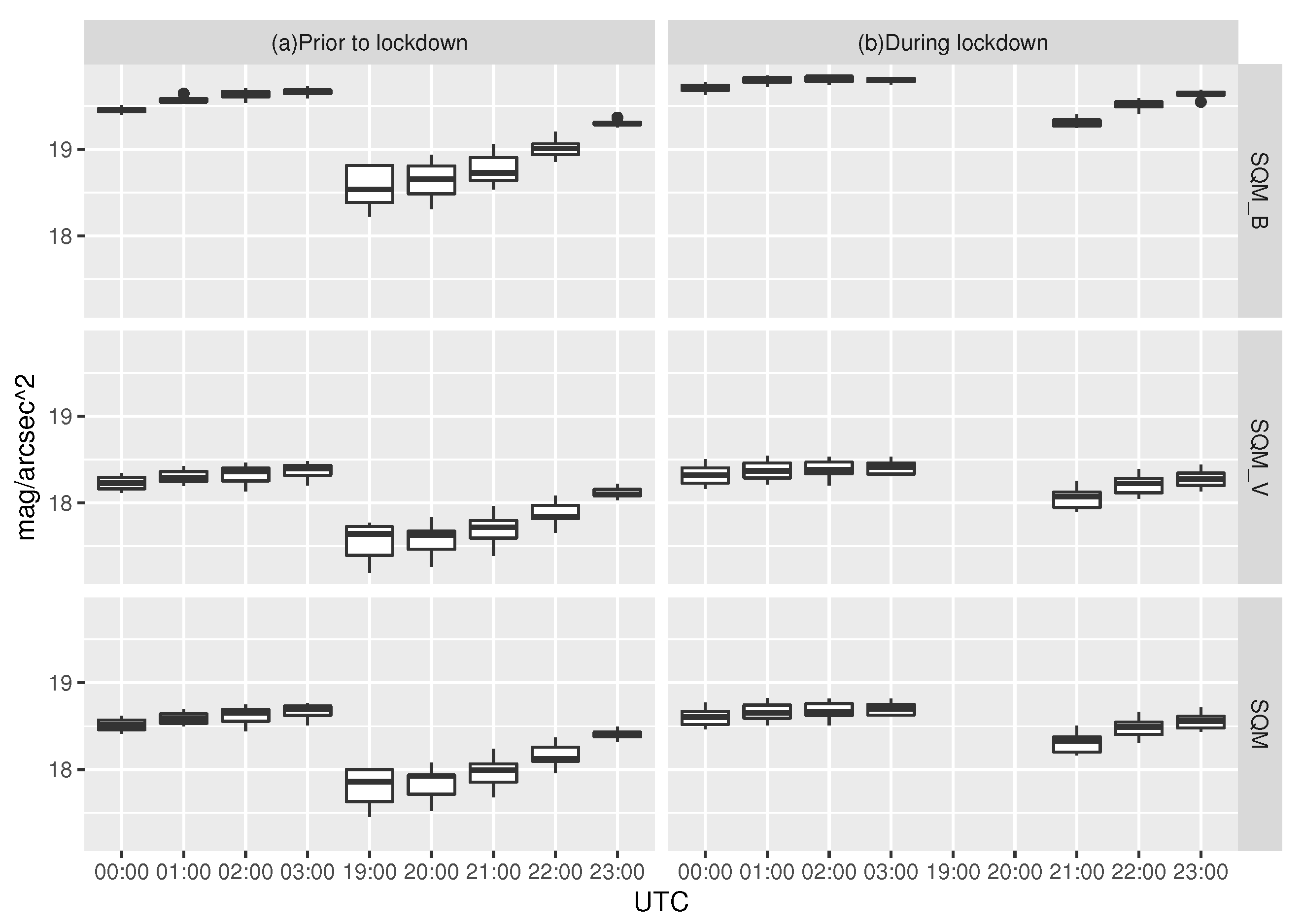
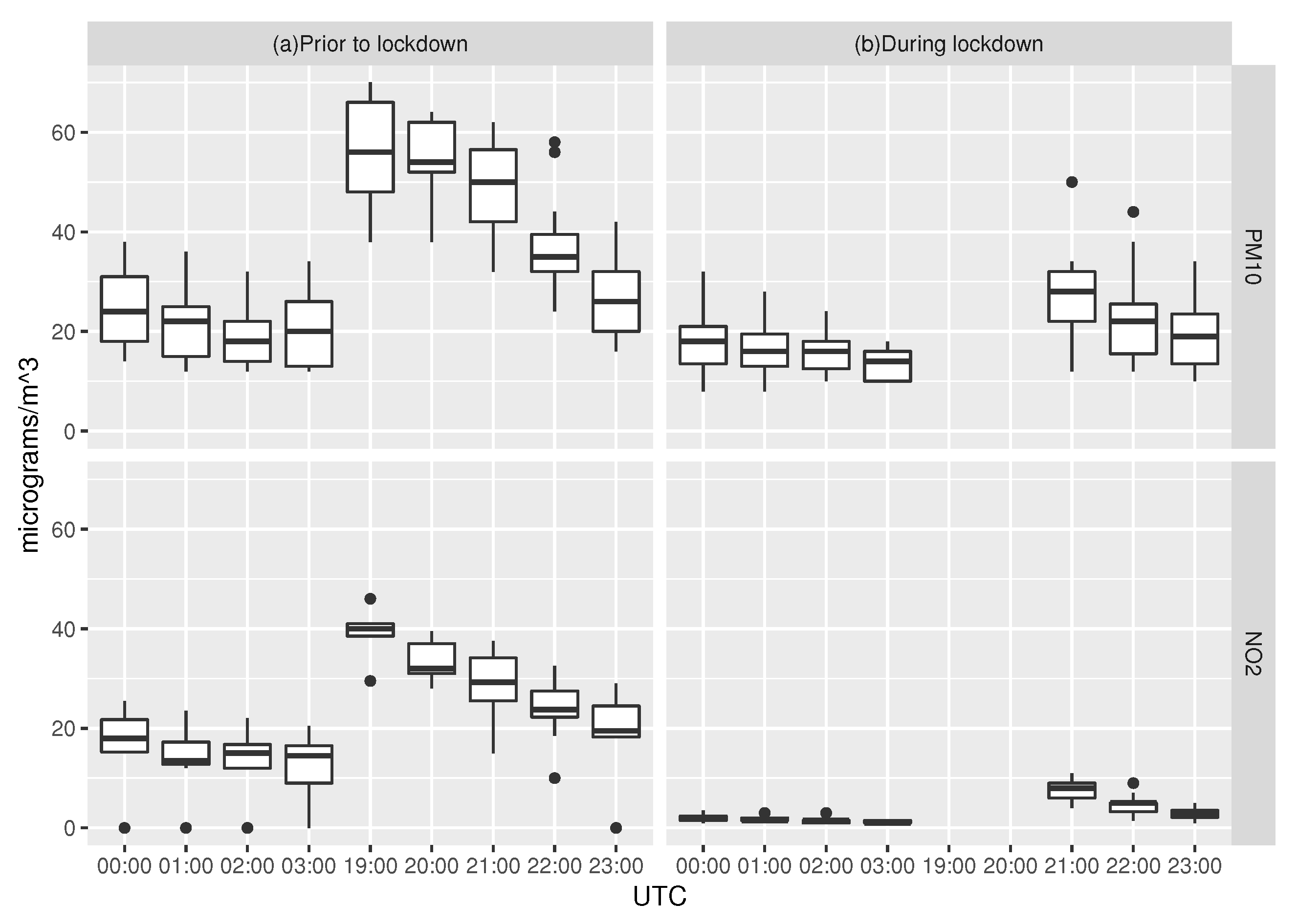
Both particulate PM10 and nitrogen dioxide concentrations were highest in the hours before midnight of the days prior to lockdown, while the lowest values occurred in the early morning and during lockdown (Figure 7 and Figure 8, Table 1). Similarly, the Granada sky was darker at zenith during the early morning hours on days of lockdown and, conversely, brighter during the first nighttime hours prior to lockdown. The differences are less if we compare the hours after 00:00. In the case of measurements obtained with the ASTMON device the differences are less significant. Only in the B band a darkening of 0.12 mag/arcsec2 is observed comparing the first hours of the night before and after the declaration of the lockdown.
The strongest correlations occur between the concentration of PM10 particles and the brightness of the sky SQM without added filter ( ρ = 0.84 ) and SQM with filter V ( ρ = 0.84 ), where ρ is the Spearman correlation index (see Table A1 and Table A2 in Appendix B). Also noteworthy is the correlation between nitrogen dioxide concentration and sky brightness in the B-band (SQMB) ( ρ = 0.81 ), and with the B-V colour index ( ρ = 0.77 ). The variables most related to the hour of the night (aka. proxy of human activity) of measurement are those corresponding to the sky brightness in all filters. This effect would dominate (higher correlation) versus air pollution (particle concentration).
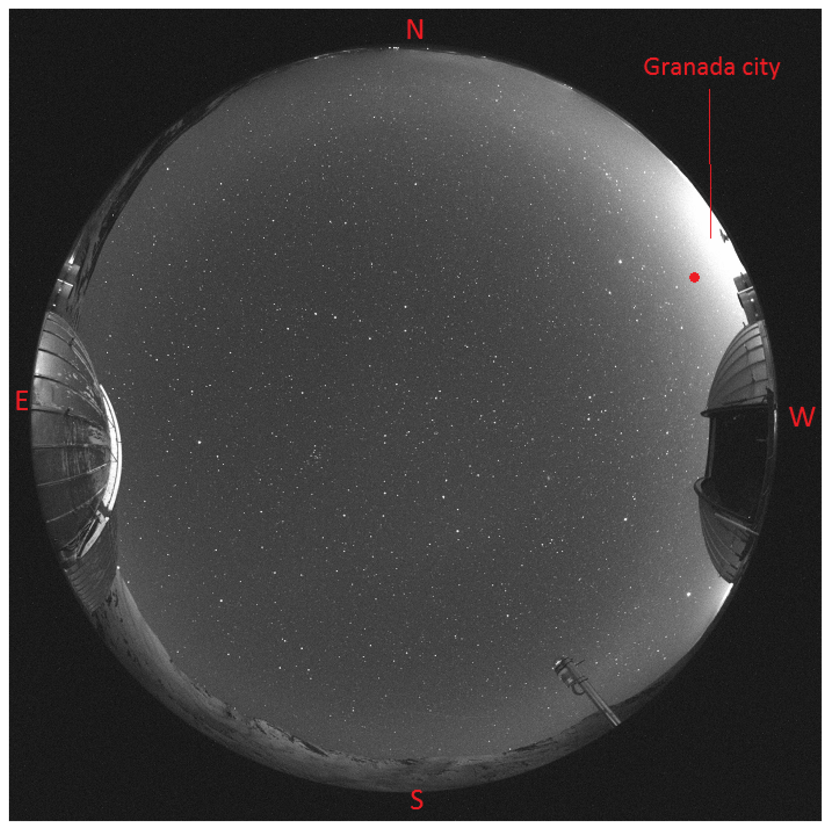
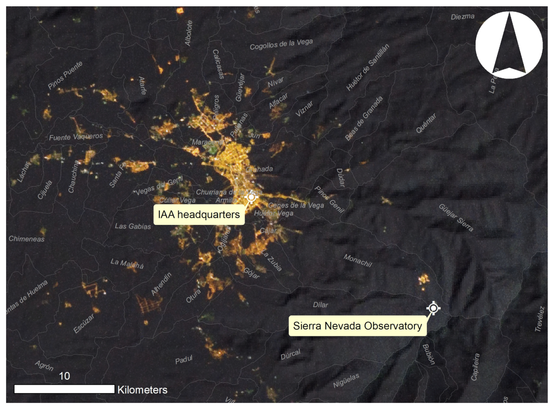
In the case of ASTMON device measurements, there are also correlations between sky brightness and air pollution variables, although they are weaker than those described above. The best correlations occur between the measurements obtained in the B band and the concentrations of NO2 ( ρ = 0.66 ) and PM10 ( ρ = 0.64 ). The brightness measurements taken from the Sierra Nevada Observatory refer to a point located 20 degrees above the horizon in the direction of the city of Granada, and from a place located 2000 m above and at a distance of 20 km. Evidently, air mass and scattering play an important role, and with a radiative transfer model these correlations could be better explained. However, for this paper we have focused on the measures obtained within the city of Granada, as they present stronger correlations, especially for PM10 particle concentration.
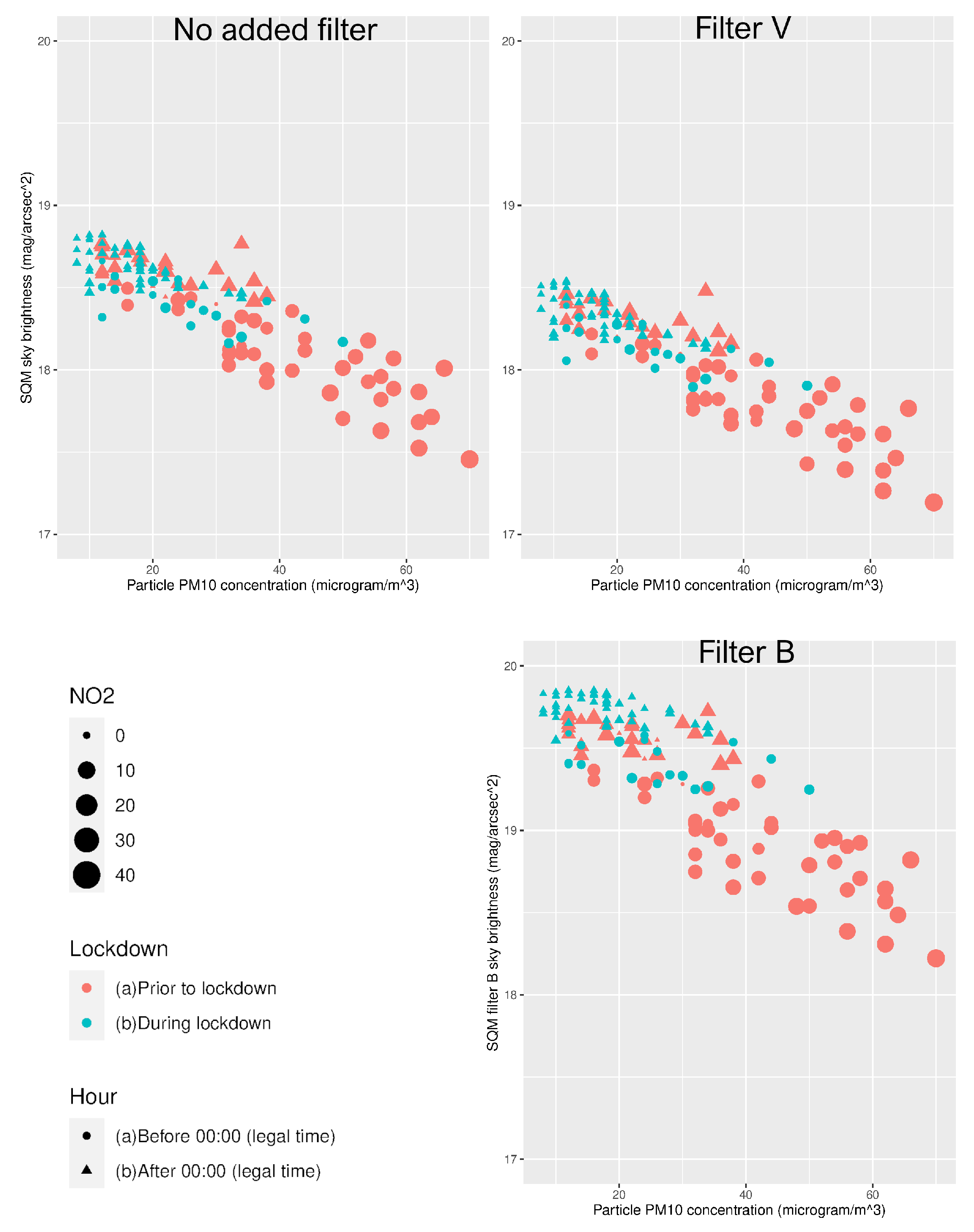
Figure 9 presents the measurements of PM10 particle concentration versus the sky brightness value (SQM without added filter, with filter V and with filter B). The upper left hand area of each graph (darker sky and lower particle concentration) is mostly occupied by measurements taken after 00:00 (legal time) during lockdown, to which the lower NO2 concentration values correspond. In contrast, the lower right zone (higher particle concentration and brighter sky) corresponds to hours before midnight on days prior to the declaration of the alarm state, and which are associated with higher NO2 concentration values. In the hours before midnight and prior to lockdown there was more traffic and activity, but it is also necessary to take into account that the concentration of nitrogen dioxide can be increased by higher levels of artificial light [37]. It should come as no surprise that the correlation between sky brightness and particle concentration is linear. The astronomical magnitude is logarithmic and the single scattering flux is proportional to e τ , where τ is optical thickness, and τ is proportional to the particle concentration [38,39,40].
The linear fitting equations for measurements of sky brightness within Granada on different filters and the PM10 particle concentration values are:
SQM (no filter)   f ( x ) = 18.91 ( 2 ) 0.0179 ( 8 ) x
SQM (filter V)   f ( x ) = 18.62 ( 2 ) 0.0176 ( 8 ) x
SQM (filter B)   f ( x ) = 20.02 ( 4 ) 0.0227 ( 1 ) x
( f ( x ) : sky brightness in mag/arcsec 2 ; x: PM10 particle concentration in μg/m3)
See Table A3, Table A4 and Table A5 (Appendix C) for errors, residuals and F-statistic.
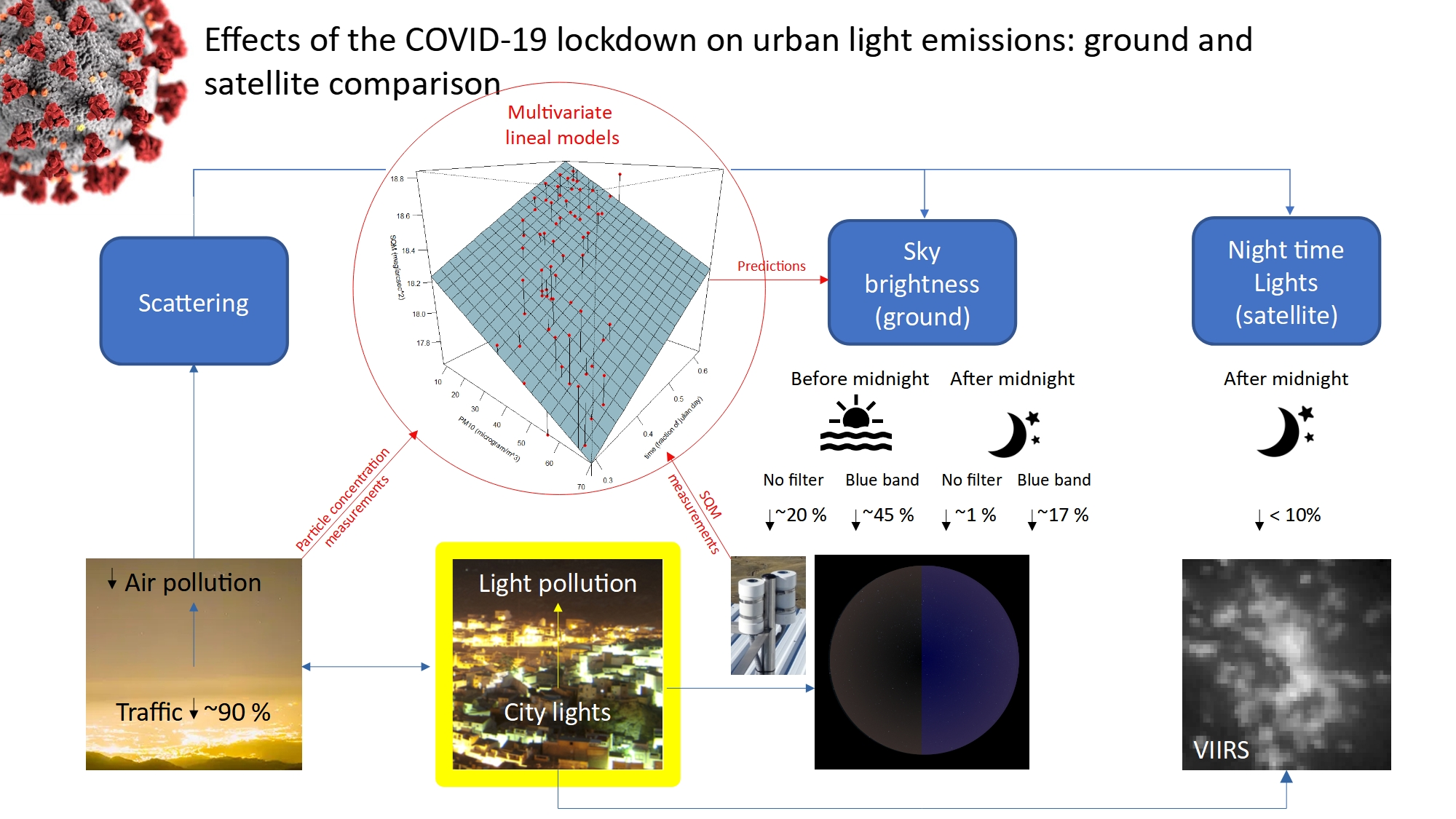
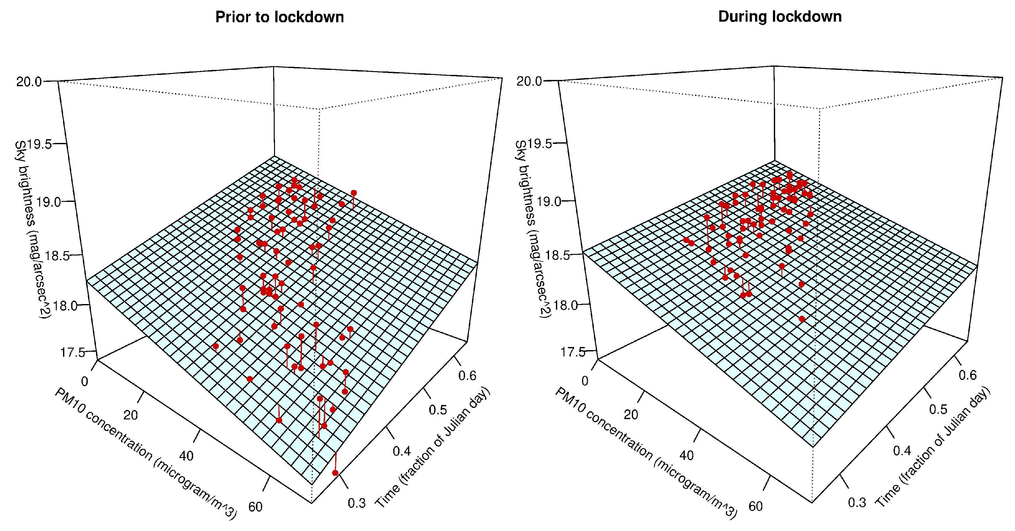
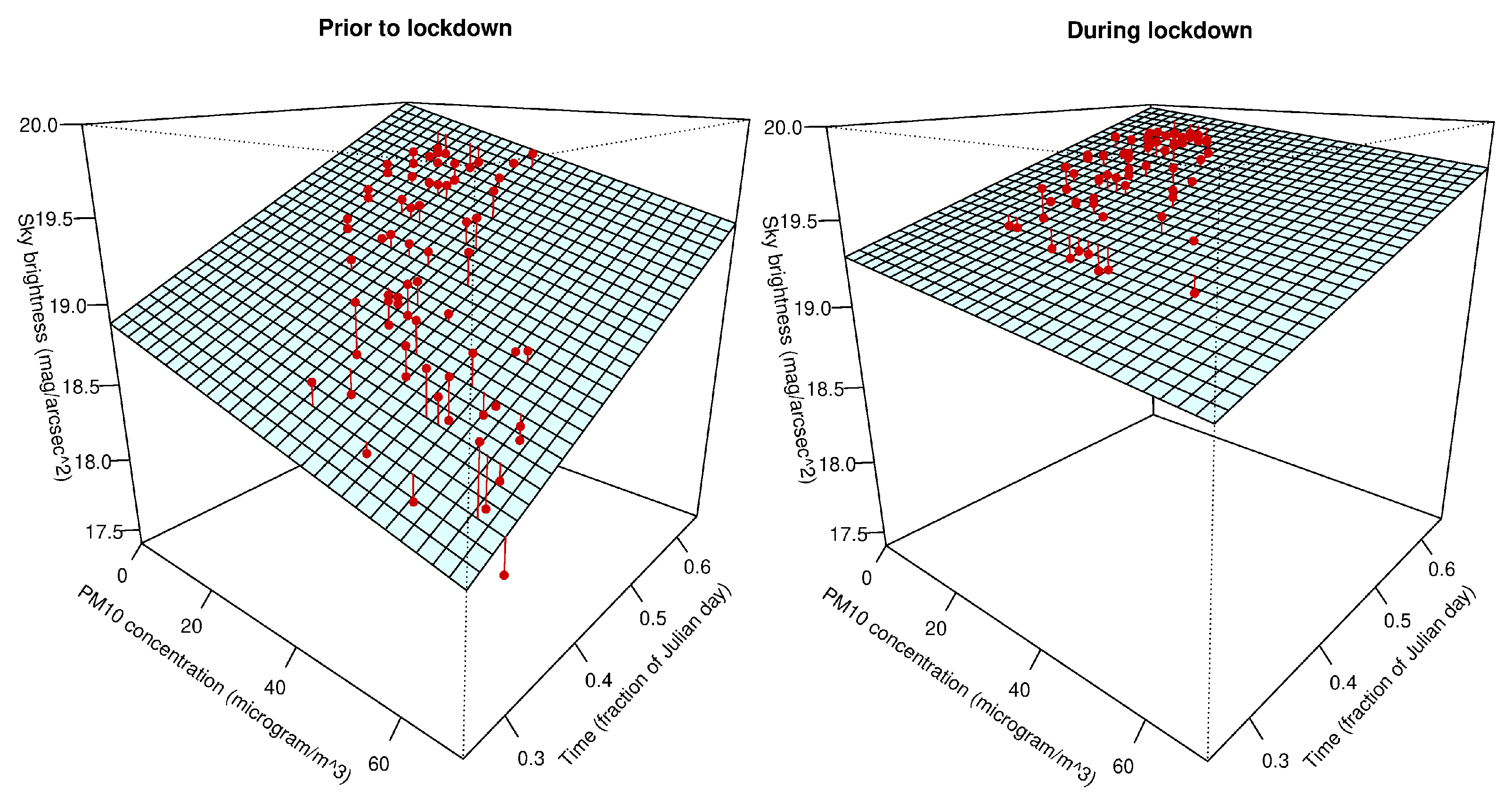
The correlation between sky brightness and particulate air pollution is also evident by performing a multivariate analysis, including time as a third dimension. Variations in urban lighting depend mainly on the time of night, and therefore can be expected to influence the sky brightness values. On the other hand, pollution levels depend on human activity, which varies throughout the night. Thus, we have calculated a model that estimates a value of sky brightness as a function of time (as a fraction of a Julian day) and particle concentration. Table A6, Table A7, Table A8 and Table A9 (Appendix C) show the values of the multivariate models for sky brightness with SQM without filter and SQM with B filter, before and during lockdown. Figure 10 and Figure 11 show the models fitting for the SQM photometer without added filter and the SQM with filter B.
The multivariate linear fitting equations for measurements of sky brightness within Granada on different filters, PM10 particle concentration values and time are:
SQM (no filter), prior to lockdown: f ( x ) = 17.79 ( 4 ) 0.0097 ( 4 ) x + 1.79 ( 2 ) t
SQM (no filter), during lockdown: f ( x ) = 18.29 ( 9 ) 0.009 ( 1 ) x + 0.94 ( 4 ) t
SQM (filter B), prior to lockdown: f ( x ) = 18.19 ( 6 ) 0.008 ( 2 ) x + 2.76 ( 5 ) t
SQM (filter B), during lockdown: f ( x ) = 18.87 ( 8 ) 0.003 ( 1 ) x + 1.71 ( 3 ) t
( f ( x ) : sky brightness in mag/arcsec 2 ; x: PM10 particle concentration in μg/m 3 ; t: time as a fraction of a Julian day. See Table A6, Table A7, Table A8 and Table A9 (Appendix C) for errors, residuals and F-statistic)

4. Comparison with Other Studies

Other studies like Elvidge et al. (2020) [31], Ghosh et al. (2020) [32] and Liu et al. (2020) [30] use mainly the VIIRS data, based on panchromatic bands with acquisition around 1:30 local time, when most of the economic activities are not longer occurring. Therefore those studies are showing only the impact of the COVID-19 on the worse possible moment of the night. In the other hand, those studies also ignore the effects of the LED transition that can produce reductions on the VIIRS intensities up to 50% [41,42]. That effect is particularly important when several months or even year are compared.
As example of this potential effect, several municipalities of Spain show decreased intensity when the median value of 2019 and 2020 is compared with the signal of April 2020. One prototypical case is the municipality of Daimiel. But a more close analysis shows how the intensity of that particular municipality has a steady decrease since November until January, with same radiance for February and march as is April. This patter can be seen on many other municipalities like Membrilla, Argamasilla de Alba, etc; all are municipalities that have recently a LED conversion. More locations can be seen on the URL https://pmisson.users.earthengine.app/view/covid-19old. When only the months of January, February, March and April are considered, the locations are reduced to a few points like airports: Madrid/Barajas (see Figure 12), Valencia/Manises, Santiago de Compostela, Alicante-Elche, etc., [43]. One of the few municipalities that shows a real decrease on street lighting is A Coruña, that have published also the details of their dimming experience [44].
This effect is considered on Jechow and Hölker (2020) [45], but because of the measurement strategy they cannot compensate of this effect.
In contrast, the multispectral measurements of the SQM stations of Granada not only can take the effects of the LED in consideration, but also can trace the variation of the intensity of the light emissions on the city of Granada with a high frequency and with much higher photometric precision.

5. Discussion

5.1. Correlation of Sky Brightness and PM10 Particle Abundance

In Figure 9 we show the sky brightness as a function of PM10 particle abundance measured in Granada from a station located around 1 km away from the site where the sky brightness measurements are taken. The altitude above sea level of the site is almost identical to that of the light pollution station.
Note that in that plot, the sky brightness measurements have not been corrected by the seasonal effects of the milky way entering the field of view of the SQM devices, but as pointed out in Appendix A this can reach a 6% contribution at most.
The correlation is obvious in the plot. Although the sky brightness can depend on many factors, it is clear that one of the main factors is the aerosol content. This is something that was expected from a physical point of view.
Garstang (1991) [38] explicitly mentioned that the sky brightness seen close to the center of a city increases with the atmospheric aerosol content, according to Garstang (1986) [39] simple radiative transfer models. Recently Kocifaj and Kundracik (2020) [40] have deepened the study of radiative transfer models and the role of particles and aerosols in the scattering of artificial light at night. Indeed, this is what we observe in Figure 9. It should be remembered that the correlation of the sky brightness in magnitudes is linear with the PM10 concentration, which also makes sense given that the single scattering flux is proportional to e τ , where τ is optical thickness, and τ is proportional to the particle concentration.

5.2. Disentangling the Effect of the Net Reduction in Light Emission from the Effect of the Decreased Aerosol Content

We have seen that sky brightness depends both on aerosol content and on the time since the beginning of the night (the higher the aerosol particle concentration the higher the brightness and the earlier at night the higher the brightness). In this section we analyze the two correlations in terms of linear correlation in two variables and we have done that with data prior to lockdown and during lockdown.
From the linear multivariate fits shown in Figure 10 and Figure 11, we can determine the night sky brightness for a reference particle concentration of 30 μg/m 3 and at 19.2 UT ( t = 0.3 as a fraction of a Julian day), prior to lockdown and during lockdown. The values are 18.04 mag/arcsec 2 and 18.29 mag/arcsec 2 before and during the confinement respectively. This means that at the same aerosol content and same time at night conditions, the confinement period was darker by 0.25 mag /arcsec 2 due to a decrease of the light output from the city. If we take into account that the brightness of the sky is around 5% higher in the period of time prior to lockdown due to higher star density getting in the detector, an approximate estimation of the decrease in the light output of the city is around 20 per cent. This percentage is probably related to the reduction in light from vehicles and from private lighting.
In the B band, the differences are more remarkable: prior to lockdown 18.77 mag/arcsec 2 ; during lockdown 19.28 mag/arcsec 2 . This means that approximately a 38% reduction in the light output of the city is derived from our data.
Note that private lighting can be a significant contributor to light pollution [46], and is usually bluer than municipal lighting, at least in some cities where cold led lighting is not extended yet. In the case of public lighting in Granada the predominant lamp is still high pressure sodium vapour, while ornamental and commercial lighting is mainly white-blue. This statement is based on the direct visual inspection made by the authors (see Section 2.4). Especially illustrative is also Figure 6, in which two images taken from the ISS at different dates and times are compared. The variation in colour and brightness of the city centre is remarkable.
This indicates that the blue band night sky brightness appears to be a better human activity indicator than the sky brightness in the visible channel. This will be even more true if the replacement of high-pressure sodium vapour with white LED continues. Furthermore, since the OI airglow line at 557 nm is mainly excluded from the B-band, the B-V index in rural areas can become a rather sensitive indicator of truly artificial light in the night sky because it excludes the dominant contribution of airglow.
Even though the outdoor human activities dropped by more than 90%, the light output of the city did not decrease by that amount, clearly pointing out that most of the city lighting does not adapt to the real use of its citizens. This shows why measurements from VIIRS are not optimal to trace the pandemic effects on the economy because of the flyby time of the satellite. Furthermore, the total insensitivity of VIIRS to the blue emission of the white LED at 450 nm makes it unreliable for the study of human activity patterns. Nor does it provide information on what is happening in the early hours of the night or at wavelengths that it cannot see. An instrument with an earlier flyby time and with a broadband spectral response is urgently needed to track changes in urban light emissions.

6. Conclusions

We found a clear decrease in light pollution (as measured in terms of sky brightness) within the city of Granada during the lockdown. Also, the sky glow from Granada as seen at a particular angle of 20 degrees outside the city, from Sierra Nevada Observatory, decreased. The observations are consistent with the idea that the decrease arose for two reasons. First, this was because of a decrease in scattered light due to the presence of fewer anthropogenic aerosols during the lockdown. In this regard, a clear correlation is found between sky brightness at several wavelength bands and PM10 particle concentration measured within the city. Outside the city at 20 degrees, the correlation coefficient with the PM10 particle concentration in Granada is lower, which makes sense given that the aerosols that contribute are not constrained to the downtown area. The other main reason for the reduction in the light pollution comes from a decrease in the net amount of light emitted by the city at the level of 20% in the visible and 38 % in the B band, probably due to a decrease in private lighting of buildings, vehicle lights and lighting of private areas, mainly observable at the start of the night. Very late at night, the flux from the city during lockdown and prior to it was almost unchanged. Satellite imagery does not show marked differences during the lockdown in terms of total light output (at the 10% precision level) because these images were obtained late at night, consistent with the ground based data, which show little change in the second half of the night. Given that outdoor activities decreased by up to 90% during lockdown, our results indicate that the light output of the city seems to be dominated by permanent lighting that does not adapt to the real use of the outdoor areas by the citizens (at least in the case of Granada), pointing out a clear waste of energy and resources.

Author Contributions

Conceptualization, M.B.-C., A.S.d.M., S.M.-R., J.-L.O., J.M.V., A.P., J.Z., J.B. and K.J.G.; Data curation, M.B.-C., S.M.-R., J.-L.O., A.G. and J.Z.; Formal analysis, M.B.-C., A.S.d.M., S.M.-R. and J.-L.O.; Funding acquisition, A.S.d.M., S.M.-R., J.-L.O., J.M.V., A.P., J.Z., J.B. and K.J.G.; Investigation, M.B.-C., A.S.d.M., S.M.-R., J.-L.O., J.M.V. and A.G.; Methodology, M.B.-C., A.S.d.M., S.M.-R., J.-L.O. and J.M.V.; Resources, A.S.d.M., S.M.-R. and A.P.; Software, A.S.d.M., S.M.-R., A.G. and J.Z.; Visualization, M.B.-C., A.S.d.M., S.M.-R. and J.-L.O.; Writing – original draft, M.B.-C., A.S.d.M., S.M.-R., J.-L.O., J.M.V. and K.J.G.; Writing – review and editing, M.B.-C., A.S.d.M., S.M.-R., J.-L.O., J.M.V., J.Z., J.B. and K.J.G. All authors have read and agreed to the published version of the manuscript.

Funding

Funding from Spanish project AYA2017-89637-R, and from FEDER, is acknowledged. We also acknowledge financial support from the State Agency for Research of the Spanish MCIU through the “Center of Excellence Severo Ochoa” award for the Instituto de Astrofísica de Andalucía (SEV-2017-0709). This work was supported by the EMISSI@N project (NERC grant NE/P01156X/1).

Institutional Review Board Statement

Not applicable.

Informed Consent Statement

Not applicable.

Data Availability Statement

The raw data of the SQM devices used for this paper can be downloaded here: https://cloud.iaa.csic.es/public.php?service=files&t=11cbaec9915b25837a3788ab4efd1c03. The air pollution data used are those collected at the Granada Congress Palace measurement station, which can be consulted on the public website: https://www.granada.org/inet/calidadaire.nsf/icayear.

Acknowledgments

This research was partially based on data taken at the Sierra Nevada Observatory, which is operated by the Instituto de Astrofísica de Andalucía (IAA-CSIC).The authors thank IAA-CSIC Computer Center and Maintenance Staff for their help in the installation of the SQM devices.

Conflicts of Interest

The authors declare no conflict of interest.

Appendix A. Measurements of the Observatory of La Sagra

The observatory of La Sagra is located in one of the darkest areas of Spain, so the low impact of light pollution allows the use of measurements taken from its location as a reference to identify the natural variations in sky brightness at the zenith between different time intervals and months. For this purpose, we have studied the data collected since 2018 by a SQM device (without added filter), selecting the valid nights of the months of February, April and May in the same time bands as for the measurements in Granada. The natural variations in sky brightness have been studied in detail by Garstang (1988) [47] and Duriscoe (2013) [48].
Figure A1 shows the average brightness of the sky from 21:00 to 22:00 and from 2:00 to 3:00 UT for a total of 30 nights (14 distributed in February and 16 in April and May). During February, in the time band before midnight the sky at the zenith is 0.28 mag/arcsec 2 brighter than in the early morning hours. In spring the situation is the opposite (although the difference is very small): from 2:00 to 3:00 is 0.05 mag/arcsec 2 brighter than from 21:00 to 22:00 UT. If we compare the same time range, we see that from 21:00 to 22:00 UT the sky is 0.27 mag/arcsec 2 darker in the spring months while from 3:00 to 4:00 UT it is 0.06 mag/arcsec 2 brighter than in February.
Figure A1. (Left): time-averaged sky brightness from the SQM photometer (no added filter) as a function of date (error bars represent the standard deviation). (Right): night-averaged sky brightness from the SQM photometer as a function of time. Photometers located at La Sagra Observatory.
Remotesensing 13 00258 g0a1
It is clear that there is a natural variation of sky brightness at the zenith due to the transit of different regions with different densities of stars. For example, in the first half of the nights in April and May the Galactic North Pole passes through the zenith region in the middle latitudes of the Northern Hemisphere. The background of diffuse starlight is minimal for this time of year and SQM devices can offer the highest values in mag/arcsec 2 . In contrast, in the second half of the nights in May and June the Galactic Equator gains height above the horizon, and richer star fields reach the zenith regions. Similarly in the early hours of February nights several bright stars pass through the zenith (e.g., Capella and Aldebaran) and influence the measurements of the SQM devices.
But to what extent are these variations perceptible in a urban environment? In order to understand this, it is necessary to put these differences into context, since in La Sagra they occur with values between 21.70 and 22 mag/arcsec 2 , in a sky of exceptional darkness, while in the city of Granada there is an artificial brightness which means that even in the best conditions the 19 mag/arcsec 2 are not reached. In terms of light intensity per unit area (mcd/m 2 ), a difference of 0.30 mag/arcsec 2 in La Sagra is approximately 0.061 mcd/m 2 , while a difference of 0.30 mag/arcsec 2 in the city of Granada is 1 mcd/m 2 . In other words, in terms of luminance, the hourly or seasonal variation of the natural brightness of the sky cannot account for more than 6.1% of the differences observed in the city of Granada [22,49].
Similarly, the hourly evolution of the average of the records of sky brightness at La Sagra for February and the months of April and May (2018–2019) can be taken as a reference of the natural variation due to the transit of different star fields through the zenith. But this is not significant in the case of the urban measurements obtained from IAA-CSIC, as the higher luminance of artificial origin masks the natural variations by almost 95%.

Appendix B. Spearman’S Correlation Coefficients

Table A1. Spearman’s correlation coefficients for sky brightness measured from IAA in Granada, air pollution and time. Time is the time measured as a fraction of a Julian day; PM10 and NO2 are the particle concentrations (between 2.5 and 10 microns) and of nitrogen dioxide (μg/m 3 ), SQM, SQMB and SQMV are the values of sky brightness without filter, with filter B and with filter V (mag/arcsec 2 ) and B.V is the color index B-V, as a result of subtracting the measurement of SQMB and SQMV.
TimePM10NO 2 SQMSQMBSQMVB.V
Time1−0.65−0.620.830.850.80.65
PM10−0.6510.69−0.84−0.77−0.84−0.44
NO 2 −0.620.691−0.69−0.81−0.68−0.77
SQM0.83−0.84−0.6910.9210.53
SQMB0.85−0.77−0.810.9210.910.78
SQMV0.8−0.84−0.6810.9110.51
B.V0.65−0.44−0.770.530.780.511
Table A2. Spearman’s correlation coefficients for sky brightness measured from OSN at ∼25° above Granada, air pollution in Granada and time. ASTMON.V, ASTMON.B and ASTMON.R are the values of sky brightness (with different Johnson filters) of the ASTMON device installed at Sierra Nevada Observatory.
TimePM10NO 2 astmon.vastmon.bastmon.r
Time1−0.61−0.540.760.830.73
PM10−0.6110.62−0.6−0.64−0.57
NO 2 −0.540.621−0.54−0.66−0.51
astmon.v0.76−0.6−0.5410.80.95
astmon.b0.83−0.64−0.660.810.76
astmon.r0.73−0.57−0.510.950.761

Appendix C. Fits of Lineal Models

The first three rows of the tables (four in the case of multivariate models) show the values of the coefficients (second column), the standard error (third column) and the statistical significance of each coefficient (third and fourth columns). A value of P r close to zero means that the predictor variable is significantly associated with the response variable.
The second section of the table shows the distribution of the fit residues: minimum and maximum values, first and third quartiles and median. Symmetric values indicate a normal distribution of the residues.
The last row of the table shows the overall quality of the fit. The residual standard error gives us an absolute measure (in the units of the response variable, mag/arcsec 2 ) of the prediction error. The determination coefficient R 2 represents the proportion of information in the data that can be explained by the model (in parts per unit). The F test evaluates the validity of the model, so a p-value close to zero means that the model is statistically significant.
Table A3. Fit of lineal model between sky brightness (SQM no added filter) and PM10 particle concentration.
Coefficients:EstimateStd. Errort ValuePr(>|t|)
(Intercept)18.9080030.024691765.78<2 × 10 16
PM10−0.0179140.000801−22.36<2 × 10 16
Residuals:
Min1QMedian3QMax
−0.37304−0.094760.025070.082790.46707
Residual standard error: 0.1401 on 135 degrees of freedom. Multiple R-squared: 0.7873, Adjusted R-squared: 0.7857, F-statistic: 499.8 on 1 and 135 DF, p-value: < 2.2 × 10 16
Table A4. Fit of lineal model between sky brightness (SQM with filter V) and PM10 particle concentration.
Coefficients:EstimateStd. Errort ValuePr(>|t|)
(Intercept)18.6151620.023941777.54<2 × 10 16
PM10−0.0175540.000777−22.59<2 × 10 16
Residuals:
Min1QMedian3QMax
−0.34851−0.098980.015890.090590.46167
Residual standard error: 0.1359 on 135 degrees of freedom. Multiple R-squared: 0.7908, Adjusted R-squared: 0.7893, F-statistic: 510.4 on 1 and 135 DF, p-value: < 2.2 × 10 16
Table A5. Fit of lineal model between sky brightness (SQM with filter B) and PM10 particle concentration.
Coefficients:EstimateStd. Errort ValuePr(>|t|)
(Intercept)20.0225820.036769544.55<2 × 10 16
PM10−0.0226600.001193−18.99<2 × 10 16
Residuals:
Min1QMedian3QMax
−0.54947−0.115640.015290.141250.47185
Residual standard error: 0.2087 on 135 degrees of freedom. Multiple R-squared: 0.7276, Adjusted R-squared: 0.7256, F-statistic: 360.6 on 1 and 135 DF, p-value: < 2.2 × 10 16
Table A6. Fit of multivariate lineal model between sky brightness (SQM no added filter), PM10 particle concentration and time (prior to lockdown).
Coefficients:EstimateStd. Errort ValuePr(>|t|)
(Intercept)17.7925100.144242123.352<2 × 10 16
PM10−0.0097090.001400−6.936 2.1 × 10 9
Time1.7927450.2243647.990 2.76 × 10 11
Residuals:
Min1QMedian3QMax
−0.27534−0.065390.005700.075550.33540
Residual standard error: 0.1161 on 66 degrees of freedom. Multiple R-squared: 0.8851, Adjusted R-squared: 0.8816, F-statistic: 254.2 on 2 and 66 DF, p-value: < 2.2 × 10 16
Table A7. Fit of multivariate lineal model between sky brightness (SQM no added filter), PM10 particle concentration and time (during lockdown).
Coefficients:EstimateStd. Errort ValuePr(>|t|)
(Intercept)18.2866600.088734206.083<2 × 10 16
PM10−0.0093530.001365−6.853 3.15 × 10 9
Time0.9364520.1446496.474 1.46 × 10 8
Residuals:
Min1QMedian3QMax
−0.244612−0.0376440.0033760.0690180.140332
Residual standard error: 0.08546 on 65 degrees of freedom. Multiple R-squared: 0.7253, Adjusted R-squared: 0.7168, F-statistic: 85.79 on 2 and 65 DF, p-value: <2.2 × 10 16
Table A8. Fit of multivariate lineal model between B-band sky brightness (SQMB), PM10 particle concentration and time (prior to lockdown).
Coefficients:EstimateStd. Errort ValuePr(>|t|)
(Intercept)18.1947920.158405114.86<2 × 10 16
PM10−0.0083630.001537−5.44 8.36 × 10 7
Time2.7626780.24639511.21<2 × 10 16
Residuals:
Min1QMedian3QMax
−0.28917−0.085990.008450.076190.37138
Residual standard error: 0.1275 on 66 degrees of freedom. Multiple R-squared: 0.9067, Adjusted R-squared: 0.9039, F-statistic: 320.9 on 2 and 66 DF, p-value: <2.2 × 10 16
Table A9. Fit of multivariate lineal model between B-band sky brightness (SQMB), PM10 particle concentration and time (during lockdown).
Coefficients:EstimateStd. Errort ValuePr(>|t|)
(Intercept)18.8651950.076974245.084<2 × 10 16
PM10−0.0033480.001184−2.8280.00623
Time1.7115200.12547913.640<2 × 10 16
Residuals:
Min1QMedian3QMax
−0.15142−0.065660.022610.054810.11129
Residual standard error: 0.07413 on 65 degrees of freedom. Multiple R-squared: 0.8226, Adjusted R-squared: 0.8171, F-statistic: 150.7 on 2 and 65 DF, p-value: <2.2 × 10 16

References

  1. NASA. Airborne Particle Levels Plummet in Northern India. 2020. Available online: https://earthobservatory.nasa.gov/images/146596/airborne-particle-levels-plummet-in-northern-india?src=nha (accessed on 16 July 2020).
  2. NASA. NASA Satellite Data Show 30 Percent Drop In Air Pollution Over Northeast U.S. 2020. Available online: https://www.nasa.gov/feature/goddard/2020/drop-in-air-pollution-over-northeast (accessed on 16 July 2020).
  3. Bui, Q.; Badger, E. The Coronavirus Quieted City Noise. Listen to What’s Left. 2020. Available online: https://www.nytimes.com/interactive/2020/05/22/upshot/coronavirus-quiet-city-noise.html (accessed on 16 July 2020).
  4. Xiao, H.; Eilon, Z.; Ji, C.; Tanimoto, T. COVID-19 societal response captured by seismic noise in China and Italy. arXiv 2020, arXiv:2005.00131. [Google Scholar] [CrossRef]
  5. Small, C.; Elvidge, C.D. Night on Earth: Mapping decadal changes of anthropogenic night light in Asia. Int. J. Appl. Earth Obs. Geoinf. 2013, 22, 40–52. [Google Scholar] [CrossRef] [Green Version]
  6. Levin, N.; Zhang, Q. A global analysis of factors controlling VIIRS nighttime light levels from densely populated areas. Remote Sens. Environ. 2017, 190, 366–382. [Google Scholar] [CrossRef] [Green Version]
  7. Rich, C.; Longcore, T. Ecological Consequences of Artificial Night Lighting; Island Press: Washington, WA, USA, 2013. [Google Scholar]
  8. Gaston, K.J.; Bennie, J.; Davies, T.W.; Hopkins, J. The ecological impacts of nighttime light pollution: A mechanistic appraisal. Biol. Rev. 2013, 88, 912–927. [Google Scholar] [CrossRef] [PubMed]
  9. Koo, Y.S.; Song, J.Y.; Joo, E.Y.; Lee, H.J.; Lee, E.; Lee, S.k.; Jung, K.Y. Outdoor artificial light at night, obesity, and sleep health: Cross-sectional analysis in the KoGES study. Chronobiol. Int. 2016, 33, 301–314. [Google Scholar] [CrossRef]
  10. Falchi, F.; Cinzano, P.; Elvidge, C.D.; Keith, D.M.; Haim, A. Limiting the impact of light pollution on human health, environment and stellar visibility. J. Environ. Manag. 2011, 92, 2714–2722. [Google Scholar] [CrossRef] [PubMed]
  11. Levin, N.; Kyba, C.C.; Zhang, Q.; de Miguel, A.S.; Román, M.O.; Li, X.; Portnov, B.A.; Molthan, A.L.; Jechow, A.; Miller, S.D.; et al. Remote sensing of night lights: A review and an outlook for the future. Remote Sens. Environ. 2020, 237, 111443. [Google Scholar] [CrossRef]
  12. NASA. Gateway to Astronaut Photography of Earth. 2020. Available online: https://eol.jsc.nasa.gov/SearchPhotos/ (accessed on 20 May 2020).
  13. Cheung, S.L.; Pun, J.C.S.; So, C.W.; Shibata, Y.; Walker, C.E.; Agata, H. Globe at Night-Sky Brightness Monitoring Network. IAUGA 2015, 29, 2257516. [Google Scholar]
  14. Zamorano, J.; García, C.; Tapia, C.; de Miguel, A.S.; Pascual, S.; Gallego, J. Stars4all night sky brightness photometer. Int. J. Sustain. Light. 2016, 18, 49–54. [Google Scholar] [CrossRef] [Green Version]
  15. Walker, C.E.; Pompea, S.M.; Isbell, D. GLOBE at night 2.0: On the road toward IYA 2009. In EPO and a Changing World: Creating Linkages and Expanding Partnerships; Astronomical Society of the Pacific Conference Series; Astronomical Society of the Pacific: Francisco, CA, USA, 2008; Volume 389, p. 423. [Google Scholar]
  16. Román, M.O.; Wang, Z.; Sun, Q.; Kalb, V.; Miller, S.D.; Molthan, A.; Schultz, L.; Bell, J.; Stokes, E.C.; Pandey, B.; et al. NASA’s Black Marble nighttime lights product suite. Remote Sens. Environ. 2018, 210, 113–143. [Google Scholar] [CrossRef]
  17. AEMET. Informe Mensual Climatológico. 2020. Available online: http://www.aemet.es/documentos/es/serviciosclimaticos/vigilancia_clima/resumenes_climat/mensuales/2020/res_mens_clim_2020_04.pdf (accessed on 14 May 2020).
  18. Mandel, E.; Murray, S.S.; Roll, J. Funtools: FITS Users Need Tools. ASCL 2011, ascl–1112. Available online: http://ascl.net/1112.002 (accessed on 1 February 2020).
  19. Joye, W.; Mandel, E. New features of SAOImage DS9. In Astronomical Data Analysis Software and Systems XII; ASP Confenrece Series; Astronomical Society of the Pacific: Francisco, CA, USA, 2003; Volume 295, p. 489. [Google Scholar]
  20. Cinzano, P. Night Sky Photometry with Sky Quality Meter. Intern. Rep. ISTIL 2005, 9, 1–13. Available online: http://www.lightpollution.it/download/sqmreport.pdf (accessed on 1 February 2020).
  21. Hänel, A.; Posch, T.; Ribas, S.J.; Aubé, M.; Duriscoe, D.; Jechow, A.; Kollath, Z.; Lolkema, D.E.; Moore, C.; Schmidt, N.; et al. Measuring night sky brightness: Methods and challenges. J. Quant. Spectrosc. Radiat. Transf. 2018, 205, 278–290. [Google Scholar] [CrossRef] [Green Version]
  22. Falchi, F.; Cinzano, P.; Duriscoe, D.; Kyba, C.C.; Elvidge, C.D.; Baugh, K.; Portnov, B.A.; Rybnikova, N.A.; Furgoni, R. The new world atlas of artificial night sky brightness. Sci. Adv. 2016, 2, e1600377. [Google Scholar] [CrossRef] [Green Version]
  23. Kyba, C.; Tong, K.P.; Bennie, J.; Birriel, I.; Birriel, J.J.; Cool, A.; Danielsen, A.; Davies, T.W.; Outer, P.N.D.; Edwards, W.; et al. Worldwide variations in artificial skyglow. Sci. Rep. 2015, 5, 1–6. [Google Scholar] [CrossRef] [Green Version]
  24. Sánchez de Miguel, A.; Aubé, M.; Zamorano, J.; Kocifaj, M.; Roby, J.; Tapia, C. Sky Quality Meter measurements in a colour-changing world. Mon. Not. R. Astron. Soc. 2017, 467, 2966–2979. [Google Scholar] [CrossRef]
  25. Unihedron. SQM-LE Operator’s Manual. 2020. Available online: https://www.unihedron.com (accessed on 1 February 2020).
  26. Bará, S.; Aubé, M.; Barentine, J.; Zamorano, J. Magnitude to luminance conversions and visual brightness of the night sky. Mon. Not. R. Astron. Soc. 2020, 493, 2429–2437. [Google Scholar] [CrossRef]
  27. Nievas Rosillo, M.; Zamorano, J. PySQM the UCM open source software to read, plot and store data from SQM photometers. Intern. Rep. UCM 2014, 1–8. Available online: https://eprints.ucm.es/25900/1/LICA_PySQM_v2.pdf (accessed on 15 January 2020).
  28. Aceituno, J.; Sánchez, S.F.; Aceituno, F.J.; Galadí-Enríquez, D.; Negro, J.J.; Soriguer, R.C.; Sanchez Gomez, G. An All-Sky Transmission Monitor: ASTMON. Publ. Astron. Soc. Pac. 2011, 123, 1076–1086. [Google Scholar] [CrossRef] [Green Version]
  29. Ayto.Granada. Calidad del Aire. 2020. Available online: https://www.granada.org/inet/calidadaire.nsf/icayear (accessed on 16 July 2020).
  30. Liu, Q.; Sha, D.; Liu, W.; Houser, P.; Zhang, L.; Hou, R.; Lan, H.; Flynn, C.; Lu, M.; Hu, T.; et al. Spatiotemporal Patterns of COVID-19 Impact on Human Activities and Environment in Mainland China Using Nighttime Light and Air Quality Data. Remote Sens. 2020, 12, 1576. [Google Scholar] [CrossRef]
  31. Elvidge, C.D.; Ghosh, T.; Hsu, F.C.; Zhizhin, M.; Bazilian, M. The Dimming of Lights in China during the COVID-19 Pandemic. Remote Sens. 2020, 12, 2851. [Google Scholar] [CrossRef]
  32. Ghosh, T.; Elvidge, C.D.; Hsu, F.C.; Zhizhin, M.; Bazilian, M. The Dimming of Lights in India during the COVID-19 Pandemic. Remote Sens. 2020, 12, 3289. [Google Scholar] [CrossRef]
  33. Kyba, C.; Ruhtz, T.; Fischer, J.; Hölker, F. Red is the new black: How the colour of urban skyglow varies with cloud cover. Mon. Not. R. Astron. Soc. 2012, 425, 701–708. [Google Scholar] [CrossRef] [Green Version]
  34. Sánchez de Miguel, A. Variacion Espacial, Temporal y Espectral de la Contaminacion Lumınica y Sus Fuentes: Metodologıa y Resultados. Ph.D. Thesis, Universidad Complutense de Madrid, Madrid, Spain, 2015. [Google Scholar] [CrossRef]
  35. Bará, S.; Rodríguez-Arós, Á.; Pérez, M.; Tosar, B.; Lima, R.C.; Sánchez de Miguel, A.; Zamorano, J. Estimating the relative contribution of streetlights, vehicles, and residential lighting to the urban night sky brightness. Light. Res. Technol. 2019, 51, 1092–1107. [Google Scholar] [CrossRef] [Green Version]
  36. Sánchez de Miguel, A.; Gomez Castano, J.; Zamorano, J.; Pascual, S.; Angeles, M.; Cayuela, L.; Martin Martinez, G.; Challupner, P.; Kyba, C. Atlas of astronaut photos of Earth at night. Astron. Geophys. 2014, 55, 36. [Google Scholar]
  37. Stark, H.; Brown, S.S.; Wong, K.W.; Stutz, J.; Elvidge, C.D.; Pollack, I.B.; Ryerson, T.B.; Dube, W.P.; Wagner, N.L.; Parrish, D.D. City lights and urban air. Nat. Geosci. 2011, 4, 730–731. [Google Scholar] [CrossRef]
  38. Garstang, R. Light pollution modeling. Publ. Astron. Soc. Pac. 1991, 17, 56–69. [Google Scholar] [CrossRef] [Green Version]
  39. Garstang, R. Model for artificial night-sky illumination. Publ. Astron. Soc. Pac. 1986, 98, 364–375. [Google Scholar] [CrossRef]
  40. Kocifaj, M.; Kundracik, F. Multi-wavelength radiometry of aerosols designed for more accurate night sky brightness predictions. J. Quant. Spectrosc. Radiat. Transf. 2020, 250, 106998. [Google Scholar] [CrossRef]
  41. Kyba, C.C.; Kuester, T.; Sánchez de Miguel, A.; Baugh, K.; Jechow, A.; Hölker, F.; Bennie, J.; Elvidge, C.D.; Gaston, K.J.; Guanter, L. Artificially lit surface of Earth at night increasing in radiance and extent. Sci. Adv. 2017, 3, e1701528. [Google Scholar] [CrossRef] [PubMed] [Green Version]
  42. de Miguel, A.S.; Kyba, C.C.; Aubé, M.; Zamorano, J.; Cardiel, N.; Tapia, C.; Bennie, J.; Gaston, K.J. Colour remote sensing of the impact of artificial light at night (I): The potential of the International Space Station and other DSLR-based platforms. Remote Sens. Environ. 2019, 224, 92–103. [Google Scholar] [CrossRef]
  43. Sánchez de Miguel, A. Pmisson/COVID-19VIIRS: COVID-19 April Variations. 2020. Available online: https://0-doi-org.brum.beds.ac.uk/10.5281/zenodo.4343646 (accessed on 10 November 2020). [CrossRef]
  44. Coque, A.; Lucas, A. Datos asociados a la atenuación de Alumbrados públicos en A Coruña durante confinamiento Covid 2020. Zenodo 2020. [Google Scholar] [CrossRef]
  45. Jechow, A.; Hölker, F. Evidence That Reduced Air and Road Traffic Decreased Artificial Night-Time Skyglow during COVID-19 Lockdown in Berlin, Germany. Remote Sens. 2020, 12, 3412. [Google Scholar] [CrossRef]
  46. Kyba, C.; Ruby, A.; Kuechly, H.; Kinzey, B.; Miller, N.; Sanders, J.; Barentine, J.; Kleinodt, R.; Espey, B. Direct measurement of the contribution of street lighting to satellite observations of nighttime light emissions from urban areas. Light. Res. Technol. 2020. [Google Scholar] [CrossRef]
  47. Garstang, R. Predictions of seasonal variations in night sky brightness. Observatory 1988, 108, 159–161. [Google Scholar]
  48. Duriscoe, D.M. Measuring Anthropogenic Sky Glow Using a Natural Sky Brightness Model. Publ. Astron. Soc. Pac. 2013, 125, 1370–1382. [Google Scholar] [CrossRef] [Green Version]
  49. LightPollutionMap. Light Pollution Map. 2020. Available online: https://www.lightpollutionmap.info/ (accessed on 16 July 2020).
Figure 1. Image from the ASTMON FoV in the V filter on 20 February 2020 at 01:16 UT. The red circle highlights the region of the celestial sphere where sky brightness measurements were taken. The instrument is situated on the roof of the main building in the middle of the two domes.
Remotesensing 13 00258 g001
Figure 2. Image of Granada city and metropolitan area taken from the International Space Station on 6 February 2012 and geo-referenced, with the gray lines delimiting different administrative regions. The white dots indicate the positions of the sensors used in this paper.
Remotesensing 13 00258 g002
Figure 3. (Left): night-averaged sky brightness from the SQM photometer (no added filter) as a function of time. (Right): night-averaged B-V index. Photometers located at IAA-CSIC headquarters in Granada.
Remotesensing 13 00258 g003
Figure 4. SuomiNPP/VIIRS-DNB observations of the Granada region using the VNP46A1 product. Cyan images are for 2018, green images for 2019. Magenta images are before the lockdown 2020 and red images for nights during the lockdown. The main isolated light pollution source in Granada, the Nevada commercial center, is marked, although it is not always visible from the satellite images because of different viewing angles on different nights.
Remotesensing 13 00258 g004
Figure 5. (Left): time-averaged sky brightness from the SQM photometer (no added filter) as a function of date. (Right): time-averaged B-V index. Photometers located at IAA headquarters in Granada. The pre-lockdown brightness is higher than in the lockdown period, especially in the hour interval before midnight (brown symbols). Each point represents the average value of the measurements for a day and a time slot, the error bars represent the standard deviation and horizontal bars represent the average. Note that we are using the standard surface brightness units in astronomy, and the magnitude scale decreases for higher brightness.
Remotesensing 13 00258 g005
Figure 6. Comparison of two images of Granada taken from the ISS at different times of the night [12]. Location thanks to the Cities at Night project [36]. By comparison of the early/left image with the late image, it can be clearly seen that the color of the lights that are off on the late one, are white lights, and ornamental lights, not general street lighting.
Remotesensing 13 00258 g006
Figure 7. Hourly measurements of sky brightness (in mag/arcsec2) with different SQM devices (with filter B, filter V and without added filter) depending on lockdown state (IAA-CSIC, Granada).
Remotesensing 13 00258 g007
Figure 8. Hourly measurements of particulate PM10 and nitrogen dioxide concentrations (in μg/m3) depending on lockdown state (IAA-CSIC, Granada).
Remotesensing 13 00258 g008
Figure 9. Sky brightness within Granada (in mag/arcsec2) versus PM10 particulate concentrations (in μg/m3) for the period prior to lockdown (red symbols) and during lockdown (green symbols) depending on time slot (triangles for the first half of the nights, dots for the second half of the nights). Symbols size represents the concentration of nitrogen dioxide. The PM10 concentration and SQM values are coinciding in time (every hour).
Remotesensing 13 00258 g009
Figure 10. Graphic representation of the multivariate lineal models between sky brightness (SQM no added filter), PM10 particle concentration and time ((left): prior to lockdown; (right): during lockdown).
Remotesensing 13 00258 g010
Figure 11. Graphic representation of the multivariate lineal models between sky brightness (SQM with filter B), PM10 particle concentration and time ((left): prior to lockdown; (right): during lockdown).
Remotesensing 13 00258 g011
Figure 12. Variation of the intensity of the Madrid/Barajas Airport Terminal TS4 during the April lockdown. More details and source code in Sánchez de Miguel (2020) [43].
Remotesensing 13 00258 g012
Table 1. Average air pollution values and average sky brightness depending on time slot and lockdown state. (P.L. = Prior to lockdown; D.L. = During Lockdown; B.00:00 = Before legal midnight; A.00:00 = After legal midnight; N.F. = No Filter).
μg/m3SQM IAA (mag/arcsec2)ASTMON OSN (mag/arcsec2)
PM10NO2N.F.BVBV
P.L./B.00:0043.3227.5918.0618.8917.7820.7119.56
P.L./A.00:0021.5014.1118.6019.5818.3021.0719.79
D.L./B.00:0025.376.1318.4019.4218.1420.8319.54
D.L./A.00:0016.981.8718.6419.7518.3521.0819.86
Publisher’s Note: MDPI stays neutral with regard to jurisdictional claims in published maps and institutional affiliations.

