Mangrove Phenology and Water Influences Measured with Digital Repeat Photography


1
ANdaman Environment and natural Disaster research center (ANED), Faculty of Technology and Environment, Prince of Songkla University, Phuket Campus, Phuket 83120, Thailand
2
School of Life Sciences, University of Technology Sydney, Sydney, NSW 2007, Australia
*
Author to whom correspondence should be addressed.
Remote Sens. 2021, 13(2), 307; https://0-doi-org.brum.beds.ac.uk/10.3390/rs13020307
Submission received: 15 December 2020
/
Revised: 13 January 2021
/
Accepted: 14 January 2021
/
Published: 17 January 2021
(This article belongs to the Section Biogeosciences Remote Sensing)
Abstract
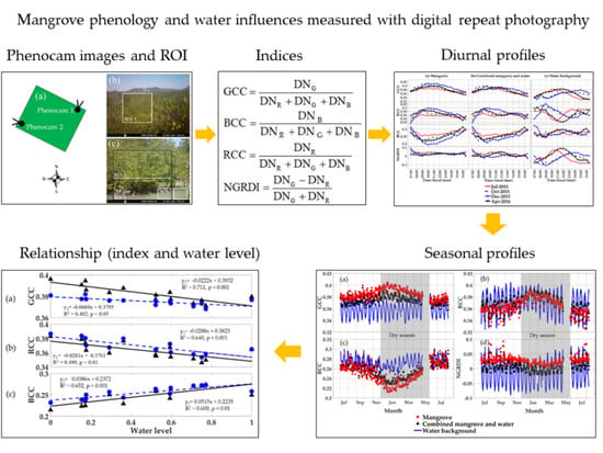
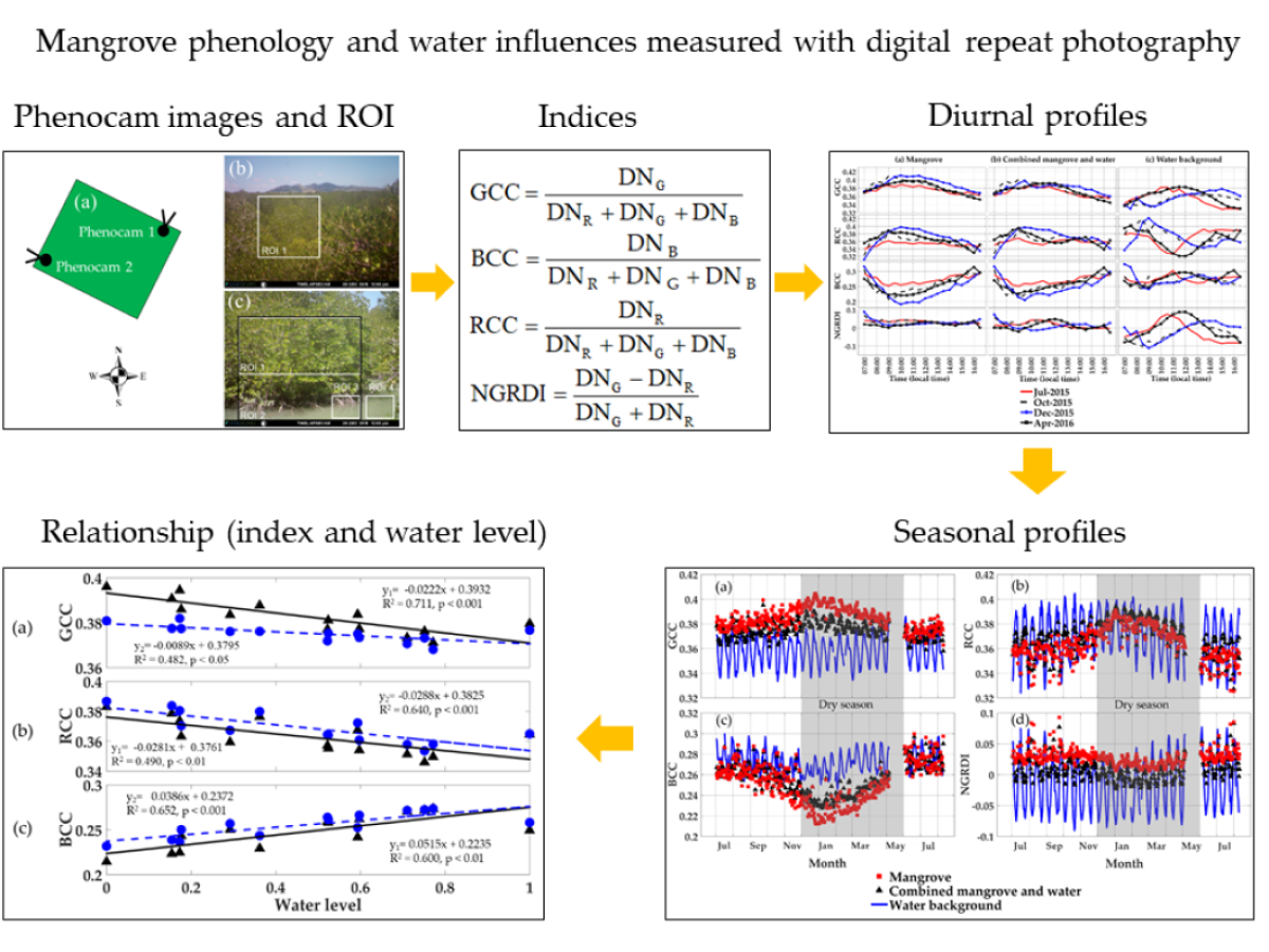
:The intertidal habitat of mangroves is very complex due to the dynamic roles of land and sea drivers. Knowledge of mangrove phenology can help in understanding mangrove growth cycles and their responses to climate and environmental changes. Studies of phenology based on digital repeat photography, or phenocams, have been successful in many terrestrial forests and other ecosystems, however few phenocam studies in mangrove forests showing the influence and interactions of water color and tidal water levels have been performed in sub-tropical and equatorial environments. In this study, we investigated the diurnal and seasonal patterns of an equatorial mangrove forest area at an Andaman Sea site in Phuket province, Southern Thailand, using two phenocams placed at different elevations and with different view orientations, which continuously monitored vegetation and water dynamics from July 2015 to August 2016. The aims of this study were to investigate fine-resolution, in situ mangrove forest phenology and assess the influence and interactions of water color and tidal water levels on the mangrove–water canopy signal. Diurnal and seasonal patterns of red, green, and blue chromatic coordinate (RCC, GCC, and BCC) indices were analyzed over various mangrove forest and water regions of interest (ROI). GCC signals from the water background were found to positively track diurnal water levels, while RCC signals were negatively related with tidal water levels, hence lower water levels yielded higher RCC values, reflecting brownish water colors and increased soil and mud exposure. At seasonal scales, the GCC profiles of the mangrove forest peaked in the dry season and were negatively related with the water level, however the inclusion of the water background signal dampened this relationship. We also detected a strong lunar tidal water periodicity in seasonal GCC values that was not only present in the water background, but was also detected in the mangrove–water canopy and mangrove forest phenology profiles. This suggests significant interactions between mangrove forests and their water backgrounds (color and depth), which may need to be accounted for in upscaling and coupling with satellite-based mangrove monitoring.
1. Introduction
Phenology is a key factor explaining climate interactions between the biosphere and the environment [1,2,3]. Jeong et al. [4] have reported shifts in phenology (the start and end of the growing season) in the Northern Hemisphere associated with increasing temperatures, and there are corresponding shifts in phenology in the Southern Hemisphere, such as in Australia [2]. Mangrove forests are a type of evergreen forest found between 40°S to 40°N [5,6]. Mangrove forests have high potential to store carbon [7,8] and play an important role in coastal erosion, nutrient, and water quality issues in estuaries and coastal areas [9]. They also serve as a location for feeding and breeding of birds, fish, and crustaceans, such as crabs, shrimp, and prawns. Despite their benefits and ecosystem services they provide, human activity has had negative impacts on mangrove ecosystems, resulting in decreasing stocks of aquatic species; pollution of water from urban development and industry; and expansion of shrimp farms, fishing, charcoal, agriculture (e.g., oil palm), and tourism [10,11,12,13,14].
The vegetation growth cycle, or phenology, includes vegetation characteristics such as leaf emergence, standing leaf crop, flowering, and leaf litter fall. In general, mangrove phenology starts with new leaf appearance, flowering, fruiting, and leaf fall, however many variations are found, depending on the mangrove species and environment. Mangrove species such as Avicennia marina in Australia [15] and Kenya [16] have the same general phenology patterns, however Ceriops decandra and Xylocarpus mekongensis in Banglasesh [17] start with leaf fall, followed by leaf appearance, flowering, and fruiting, which is also similar to Sonneratia alba at Australian sites in Queensland [18]. Furthermore, the phenology of Kandelia ÿ picula in Japan [19] begins with flowering, then leaf appearance, leaf fall, and fruiting. In Thailand, Christensen and Wium-Andersen [20] reported that leaf production for Rhizophora ÿ piculate was maximal in May–June, followed by flowering of buds during August to November, developing into full flowering between December to February in the following year, while there was no distinct seasonal variation of leaf fall throughout the year.
The study of mangrove phenology is important to understand the mangrove forest ecosystem, because mangroves are vulnerable to climate change (temperatures, sea levels, storm cycles, etc.) [21]. Changes in mangrove phenology affect primary productivity and consumer organisms in the mangrove ecosystem [18], where energy transfer starts primarily after leaf fall [20,22,23]. Leaf fall provides food for crustaceans and fish, who in turn provide food for bigger animals [24]. Therefore, if the timing of leaf fall has shifted, activities consequential to the timing and magnitude of litter fall may be changed. Understanding the mangrove phenology is also helpful in selecting suitable dates for replanting.
Traditional mangrove phenology studies use visual observations, which are not as suitable for large areas and over long recording times. An alternative approach to studying vegetation phenology involves the use of remote sensing data due to the ability to acquire high temporal resolution images over large areas, from regional [25,26,27] to global scales [28,29,30]. Nevertheless, cloud interference in tropical areas can severely limit the use of satellite data for phenology studies, particularly when much of the mangrove forest growth occurs during the monsoon or wet season [31]. There have been some mangrove phenology studies carried out with remote sensing data [32,33]. Songsom et al. [33] used the Moderate Resolution Imaging Spectroradiometer (MODIS) enhanced vegetation index (EVI) with 250-m resolution to monitor mangrove phenology in Southern Thailand. Their results showed significant seasonal changes over the year-round evergreen mangroves. However, there were limitations resulting from the coarse spatial and temporal resolution of the satellite data [31,34].
Digital repeat photography imaging, also known as digital time lapse camera or phenocam imaging, is another option that can be used to monitor vegetation phenology. The advantage of ground-based digital imaging is that data can be captured continuously and at very high temporal resolutions, regardless of cloud conditions [31,34,35]. Time series photography can capture pheno-phases of vegetation, while long-term digital photography can record phenological activity across multiple years, which may include drought and wet years [31,36,37]. In addition, digital photography is also used to validate remote sensing data with the observed ground-level vegetation phenology [38,39,40,41,42,43,44]. The digital image processing algorithm can be trained to detect important events such as the date of flowering, duration of flowering, peak greenness, and leaf senescence [45]. Moore et al. [3] showed the value of high-performance digital imaging and remote sensing to evaluate the functioning of Australia’s terrestrial ecosystems (tropical rainforest, tropical savanna, and temperate evergreen forest environments). Some studies have used digital image analysis to evaluate biophysical characteristics of vegetation, such as the biomass [46] and leaf area index [47]. The cameras can be used to map specific vegetation species. The study of phenological characteristics at the species level is important because different species are likely to be governed by different phenological control factors [31,48]. The various vegetation types that have been studied with digital cameras technology include grassland [46,49,50,51], deciduous broadleaf forest [34,44,47,50,51,52,53,54], temperate freshwater wetland [31], evergreen broadleaf forest [31,50,55], mixed deciduous forest [31,36] and tropical rainforest [35] environments. However, the knowledge of mangrove phenology based on digital photography is very limited [56], with such studies yet to be carried out over an entire growing season, particularly in equatorial environments. Additionally, the vegetation index which may be successful in assessing terrestrial phenology (green chromatic coordinate or excess green [34] values), may not be helpful for mangrove forests. Several vegetation indices may be needed to characterize mangroves, due to the influences of water and changes in water level and salinity, differences in wet mangrove soils compared to forest soils, and different forms of canopy structural complexity [6].
Rainfall is a main driving factor in upland tropical forests, where changes in seasonal vegetation are directly driven by the seasonality of the rainfall [30,57]. Songsom et al. [33] reported that high cumulative rainfall induced a later green-up date for mangroves in Southern Thailand. During periods of increasing rainfall, water levels rise, while they are lower during the dry season; however, it is not known in which ways water levels influence the remotely sensed observations of mangrove vegetation from satellites. In the dry season, as well as at diurnal low tide levels, the mangrove canopy background will consist of more shallow water with greater mud and soil exposure, while at high tide and in the wet season, the mangrove canopy background would have higher water levels. There are studies on the relationship between sea level rise and the expansion of mangrove areas [58,59], and both rainfall and water level are known to induce changes in salinity levels, both seasonally and during tidal cycles, with potential stress on mangrove forests.
In this study, we investigated the green leaf phenology and water background seasonal patterns of a mangrove forest located in Phuket province, Thailand, using two in situ time lapse digital cameras (phenocams). The objectives of this study were to (1) investigate the mangrove forest and water background diurnal and seasonal characteristics across wet and dry seasons, and (2) to assess the influence and interactions of tidal and seasonal water dynamics on phenocam-derived spectral indices.
2. Materials and Methods
2.1. Site Description and Phenocam Details
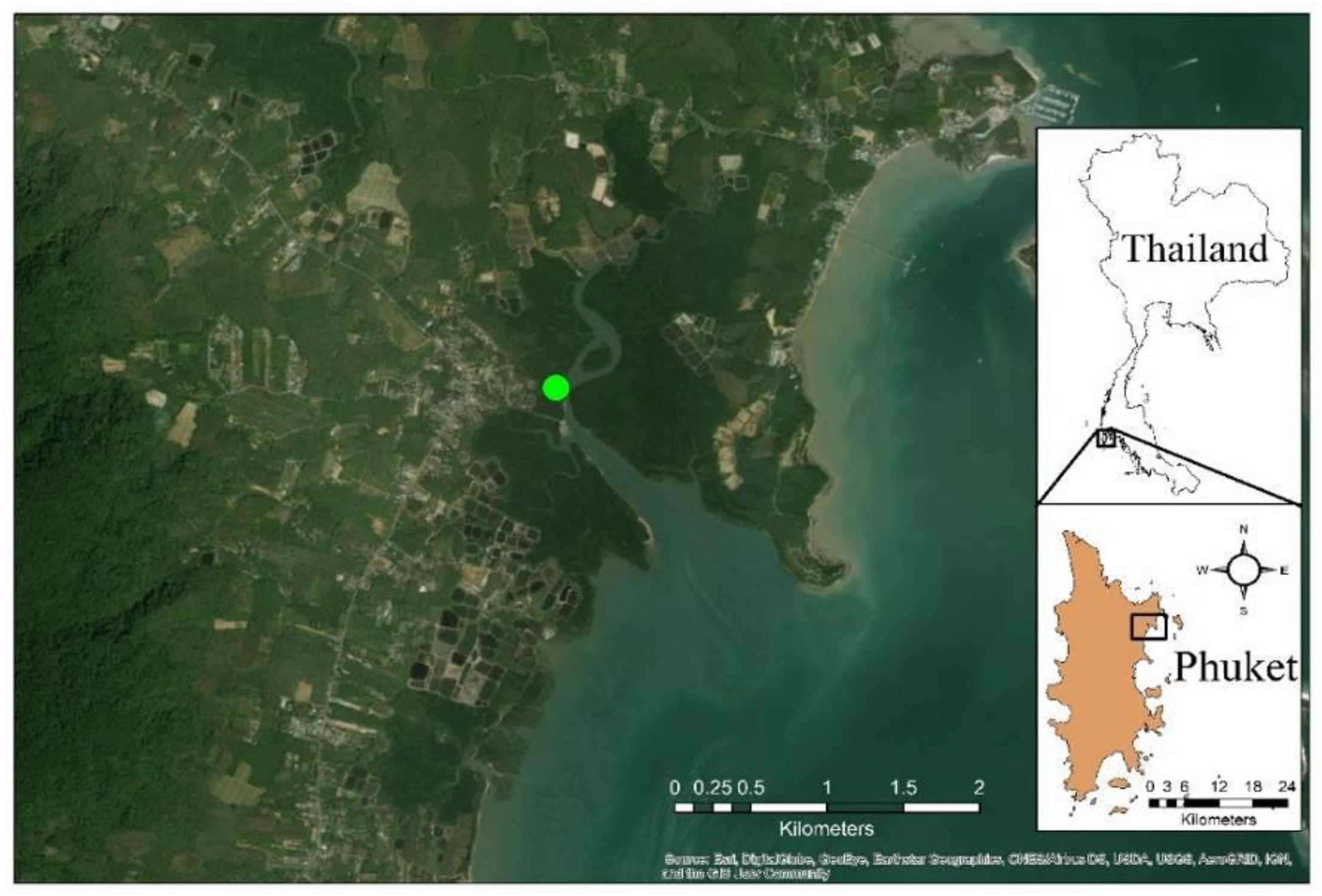
The study area is located in Bangrong Bay (8.052°N and 98.415°E), along the Andaman Sea in Phuket province, Southern Thailand (Figure 1). This site is the largest (~3 km2) remaining mangrove area in Phuket province, with Rhizophora apiculata as the dominant species. The cumulative annual rainfall is 2500 mm, with the wet season extending from May to November and the dry season from December to April. The mean annual temperature is 28 °C, with minimal seasonal temperature variation.
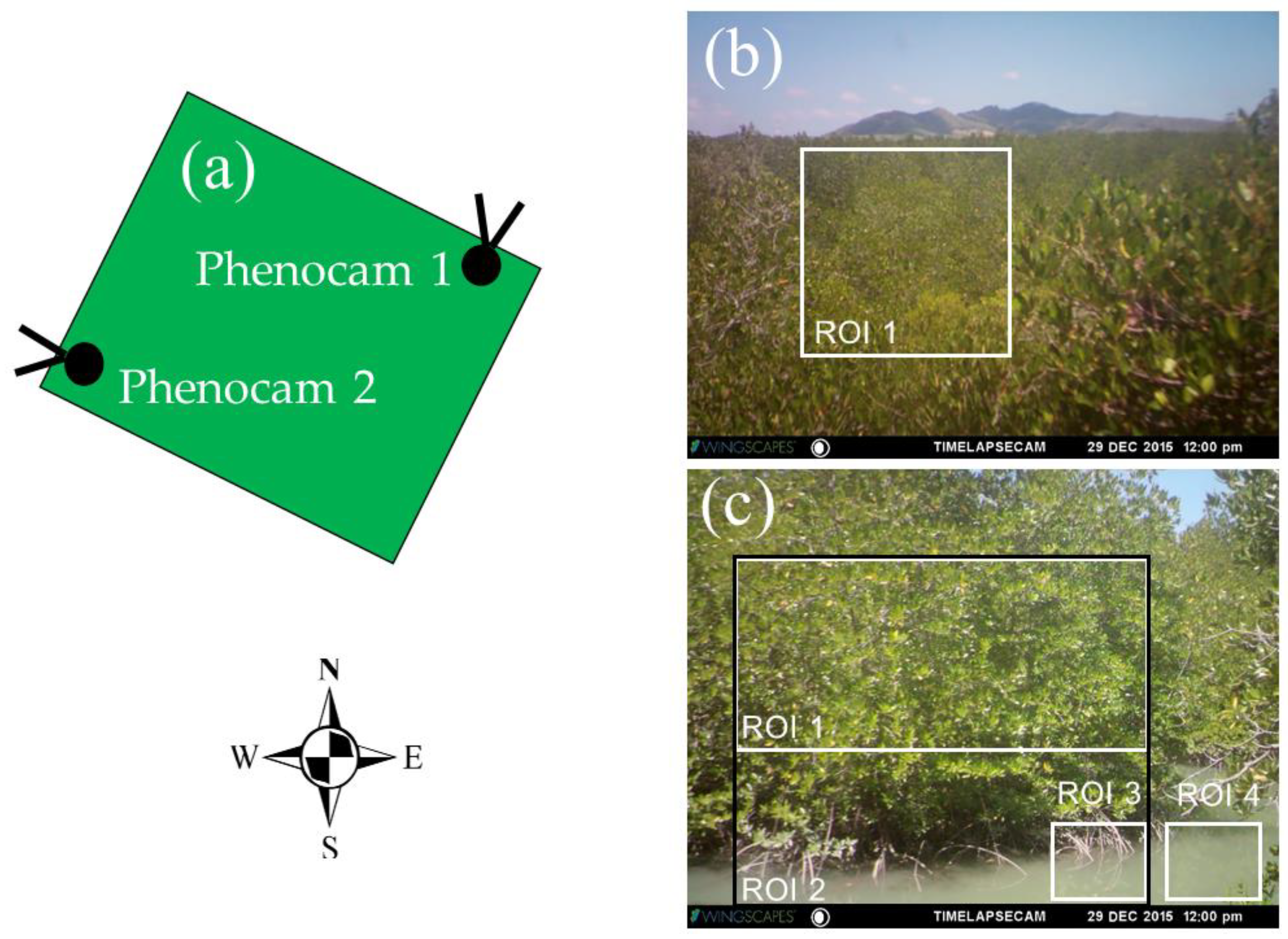
To study the mangrove phenology, two WingscapesTM time lapse RGB cameras (phenocams) were installed on a mangrove observation tower (8.052°N, 98.415°E) (Figure 2). The heights of phenocam-1 and phenocam-2 were 15 and 5 m above mean sea level, respectively. The orientation of phenocam-1 was north-facing and that of phenocam-2 faced to the west (Figure 2a). The view angles of phenocam-1 and phenocam-2 were set at 5° and 3°, respectively. The observation period was from July 2015 to August 2016, and both phenocams captured images every 30 min [36,44] from 07:00 to 16:30 local time (GMT + 07 h). The focal length was set to infinity for both phenocams. All images were saved as JPEG files and contained red (R), green (G), and blue (B) channels containing 2592 × 1944 pixels. Due to the limitations of the memory cards of the phenocams (8 Gigabyte), the data were collected during field site visits every month.
2.2. Data Used
2.2.1. Phenocam RGB Indices
The red–green–blue (RGB) digital numbers (DNs) from the phenocam images were extracted, separated, and transformed into RGB chromatic coordinate indices, including the green chromatic coordinate (GCC) index, red chromatic coordinate (RCC) index, and blue chromatic coordinate (BCC) index (Equations (1)–(3), Table 1). The DN of each color channel was very sensitive to scene illumination and the DNs divided by the sum of all 3 color DNs served to normalize scene illumination variations. The GCC index is the most commonly used index for studying phenology using phenocams [44,47,51,60] due to its sensitivity to green leaf color [40]. The normalized green–red difference index (NGRDI) [61] (Equation (4)) is functionally equivalent to the green/red ratio [62] and was developed from the formula structure of the normalized difference vegetation index (NDVI) and simple ratio (SR) by substituting the green band for the near-infrared (NIR) band.
The GCC and NGRDI greenness indices were used in this study to monitor mangrove phenology and assess the influences of soil, mud, and standing water. Positive NGRDI values indicate more green leaves in the image, while negative values indicate a high presence of soil, mud, or water cover [63]. The RCC and BCC indices were used to better characterize the red and blue color features of the mangrove, water background, and exposed soil regions.
Different regions of interest (ROI) were delineated to represent the mangrove forest, water background, and combined mangrove–water canopy (Figure 2b,c). The pixel DNs within each ROI were averaged and used to calculate the RGB chromatic coordinate and vegetation indices for the 30 min images (7:00 to 16:30 local time). This resulted in 20 values per day for each color index. ROI 1 from both phenocams represented the mangrove forest, while ROI 2, ROI 3, and ROI 4 from phenocam-2 represented the mangrove–water canopy, water level detection, and water background, respectively.
2.2.2. Rainfall and Water Level Influences
We analyzed rainfall and water tide levels as potential drivers of mangrove phenological growth. Daily rainfall data were obtained from the NASA (National Aeronautics and Space Administration) precipitation estimate product TRMM-3B42 (Tropical Rainfall Measuring Mission-3B42) at 0.25° resolution and downloaded from https://disc.gsfc.nasa.gov/. This product provides merged infrared precipitation data (mm/h) with a 3-hourly temporal resolution, from which we derived daily precipitation values. The closest water level gauge data were 30 km from the study site. It was also not located in a tidal creek environment and so data from it would not have been of great value, not only because of the magnitude but also the flushing time of the tidal creek at the study site. Thus, to avoid uncertainties due to timing lags and elevation effects on actual water levels at our site, we derived sub-daily local estimates of water tide levels by monitoring the relative water level observed from the phenocam-2 data (ROI 3, Figure 2c). The relative water level was then normalized from zero to one for further analysis. The study area is located near the equator, at 8° N latitude, with a fairly constant day length through both wet and dry seasons. We, therefore, did not use solar radiation data directly as drivers of mangrove growth, but instead used rainfall data for empirical inverse estimates of sunlight. The sky is generally overcast during the wet season, whereas it is clearer in the dry season (winter), even though the solar angle is lower (+68.5° at winter solstice).
2.3. Diurnal and Seasonal Analysis
We analyzed the diurnal mangrove forest canopy, water background, and the combined mangrove–water canopy with the phenocam RGB color indices from 07:00 to 16:30 (local time) and at four phenology periods of the year. The periods included 14–16 July 2015, 18–20 October 2015, 29–31 December, and 7–9 April 2016, representing the dry season (December), wet season (July), and dry-to-wet (April) and wet-to-dry (October) transitional periods, respectively. We averaged three consecutive days to generate the sub-daily phenocam color indices and water level profiles.
To generate seasonal mangrove profiles, the 30 min sub-daily phenocam data were composited to daily values by averaging mid-day, near-solar-noon values, from 10.00 to 14.00 (local time), and by selecting the 90th percentile. The observations near solar noon both reduced sun angle variation and produced a more consistent daily phenology measure. Additionally, a three day moving average was applied to smooth the time series data [36,44]. The peak of the growing season was used as a key descriptor of the mangrove forest phenology.
The diurnal, daily, and seasonal data were used to analyze relationships between the phenocam color indices and tidal water levels. Cumulative daily rainfall data were computed and related to mangrove forest leaf flush periods. Linear regression and Pearson’s correlation were used to explain the relationships across the RGB color indices and water levels.
3. Results
3.1. Diurnal Profiles of the Mangrove Forest
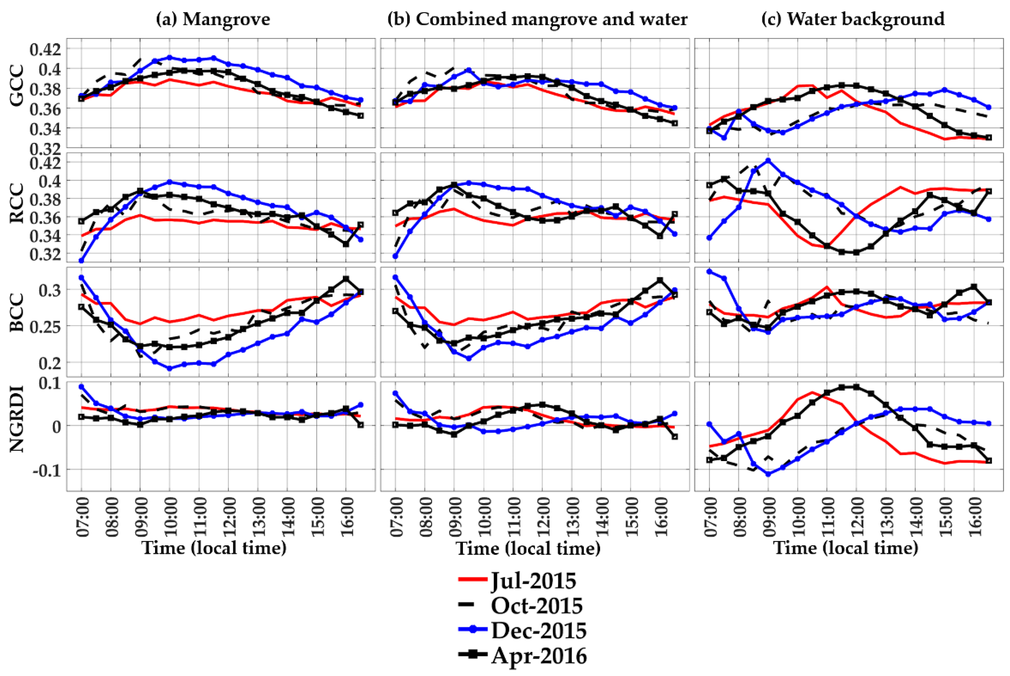
The phenocam-2 diurnal profiles, representing the mangrove forest, water background, and mangrove–water canopy ROIs (Figure 2), are shown in Figure 3 for the four RGB color indices and four seasonal periods of the year. The mangrove forest exhibited strong diurnal variation, with sharply increasing GCC values in the morning and peak values at mid-morning (10:00–11:00 h) (Figure 3a). The RCC profiles showed similar diurnal patterns as for GCC, while the BCC profiles were inversely related to those of GCC and RCC. The NGRDI profiles were relatively stable throughout the day and appeared to be the least affected by diurnal sun angle variations (Figure 3a).
Profile variations across the 4 seasonal periods of the year were pronounced for the GCC, RCC, and BCC indices and were smaller for NGRDI. The highest GCC and RCC values occurred in the dry season (December) period, while the lowest GCC and RCC values were in the wet season (July) period. BCC values, and to a lesser extent NGRDI values, were seasonally out of phase, with the highest values occurring in the July wet season period (Figure 3a).
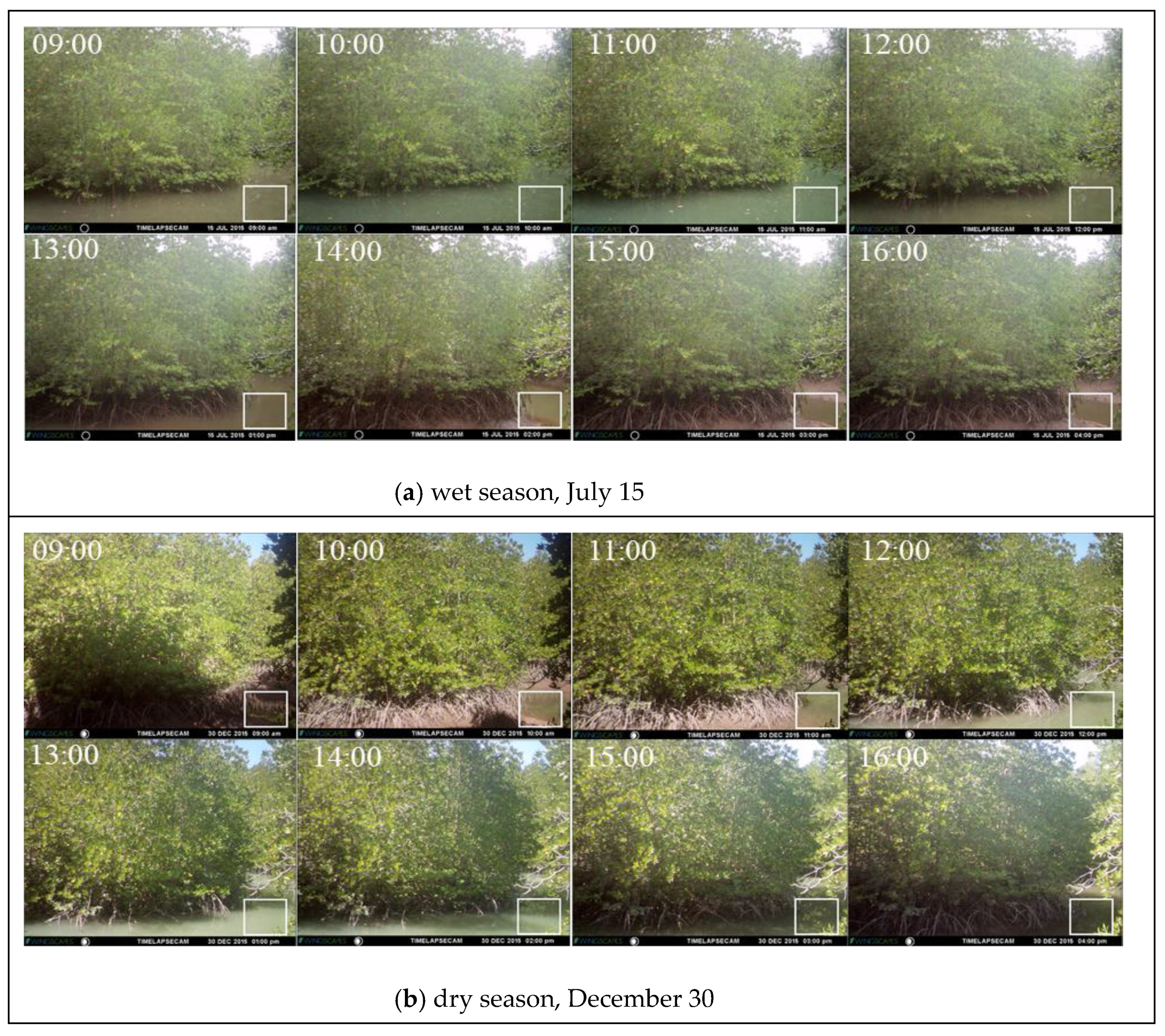
The high GCC and RCC values seen in mid-morning may be attributed to the west-facing phenocam view orientation, in which the mangrove forest was observed in the backscatter (sunlit) direction, with minimal shading and close to the hot spot at mid-morning. This was followed by forward scatter observations in the afternoon, when the mangrove forest becomes increasingly shaded, causing GCC and RCC to decrease while BCC increases. The diurnal pattern of sunlit-to-shaded mangrove forest images can be seen in the dry season (December) phenocam image sequence (Figure 4). Thus, the diurnal anisotropy was much greater in the dry season due to the greater occurrence of sunny days (strong back- and forward scatter conditions) relative to the wet season, when most days are cloudy and diffuse diurnal radiation variations are much smaller.
3.2. Diurnal Profiles of the Water Background
There were significant diurnal RGB color index variations for the water background underneath the mangrove forest due to variations in tidal water levels, sediments, and soil exposure (Figure 3c and Figure 4, ROI 3). The sample diurnal profiles over 4 periods of the year corresponded very well with the apparent colors of the water observed in the phenocam diurnal images (Figure 4). The greenness index values (GCC, NGRDI) peaked at 10:00 to 11:00 in the July wet season period, and also peak at 13:00 to 15:00 in the dry season (December), both of which matched the apparent “green water” color seen in the phenocam images at these times (Figure 3c and Figure 4a,b).
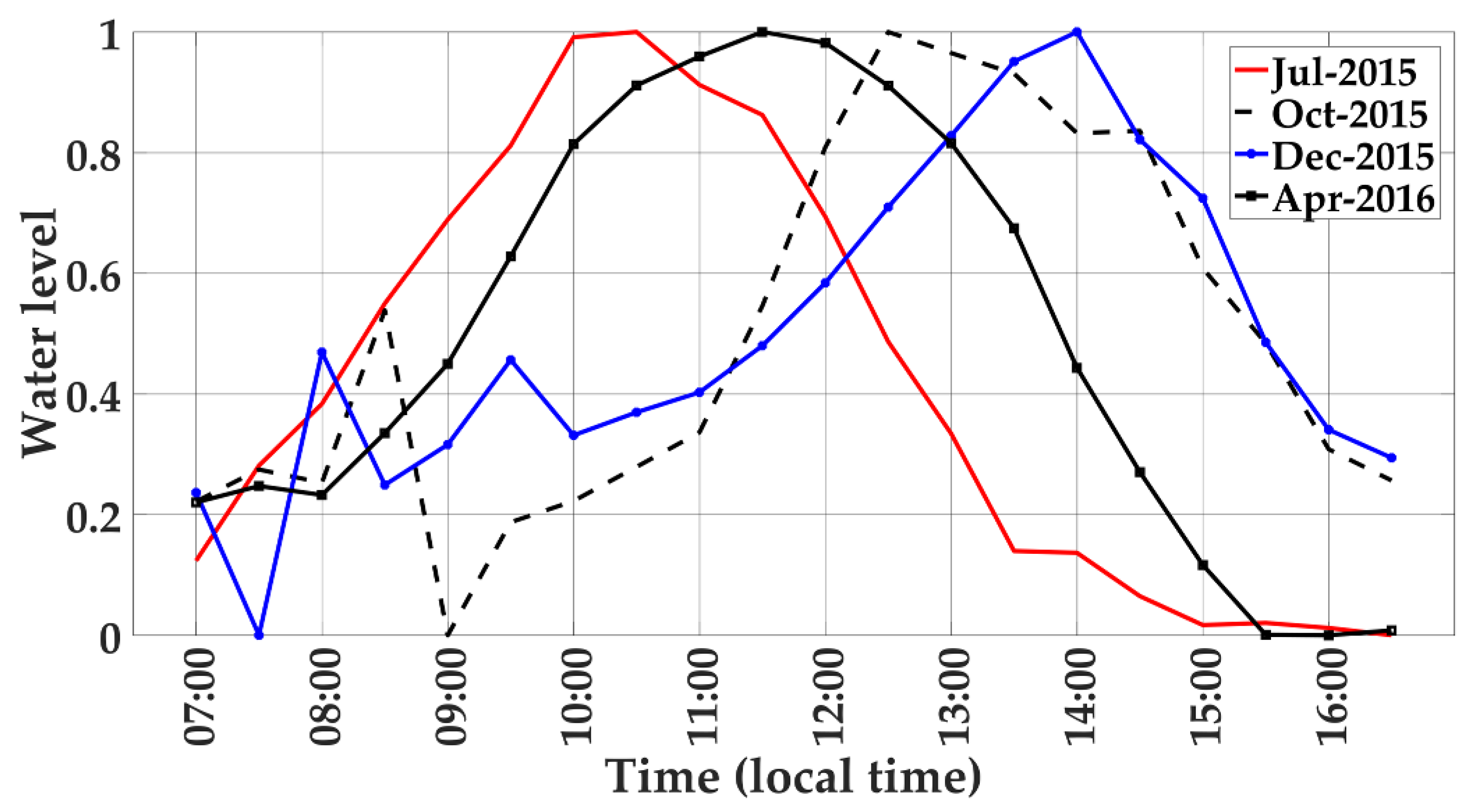
The diurnal RGB color index values of the water also appeared to be synchronized with water level variations (Figure 5). The diurnal greenness (GCC and NGRDI) values positively tracked diurnal water levels across all 4 seasonal periods. For example, in the wet season period (July), water levels increased from early to mid-morning and were maximum at 10:00, coincident with GCC and NGRDI peak values at 9:30 to 10:00. In April, the GCC, NGRDI, and water levels peaked at 11:30, while in October their peaks occurred at 12:30. The dry season period (December) showed peak GCC and NGRDI values at 15:00, nearly coincident to the 14:00 water level peak.
Diurnal BCC values were also positively related with water levels, but with smaller variations relative to GCC values (Figure 3c and Figure 5). Diurnal RCC values of the water, on the other hand, varied inversely with diurnal water levels across all seasonal periods (Figure 3c and Figure 5). The diurnal behavior of RCC can also be linked to the color of the water (Figure 4). In the wet season (July), RCC values of the water are at their lowest at 11:00 and increase in the afternoon, corresponding with phenocam images displaying increasing brownish water, mud, and exposed soil. Thus, water color and water level co-vary with RCC values. The diurnal water RGB index color variations were of the same magnitude as those from the mangrove forest (Figure 3a,c). The GCC values of the water varied from 0.33 to 0.38, while the GCC values from the mangrove forest ranged from 0.35 to 0.41. The RCC values had a stronger diurnal-seasonal range of 0.32 to 0.42 over water than in mangrove forests (0.32 to 0.40), while BCC values had a larger range of values (0.18 to 0.32) in the mangrove forest than in the water (0.24–0.32). NGRDI values were twice that in the water (−0.12 to +0.10) than found in the mangrove forest (0 to 0.09).
3.3. Diurnal Profiles of Combined Mangrove–Water Canopy
The diurnal profiles of the combined mangrove–water canopy RGB color indices are shown in Figure 3b. The influence of the added-water signals was to lower the overall GCC values relative to mangrove forest. This influence was seasonally associated with a greater GCC decrease in the dry season (December) and only a minor decrease in the wet season (July). The dry season had the lowest water levels, with greater likelihood of muddy water and exposed soil, which would lower the GCC to a greater extent than in the wet season. The mangrove–water canopy GCC may be approximated as a linear combination of the relative proportions of mangrove forest and water within the ROI, and in our case the fractional area of the water background in the ROI was approximately 20%.
In contrast to GCC, RCC values were minimally impacted by the water present in the combined mangrove–water canopy relative to the mangrove forest (Figure 3b). The BCC values slightly increased in the combined mangrove–water canopy relative to the mangrove forest only, as the water BCC values were relatively higher than those for the mangrove forest. As with the mangrove forest diurnal profiles, the BCC profiles of the combined mangrove–water canopy were inversely related to the patterns of GCC and RCC indices, such that the BCC values were highest in the wet season (July) and lowest in the dry season (December).
The combined mangrove–water canopy diurnal NGRDI profiles generated slightly lower NGRDI values relative to the mangrove forest, but also displayed much greater water diurnal variations and peak values that coincided fairly well with the normalized water levels (Figure 3b and Figure 5). Thus, the presence of water in the mangrove forest enhanced the NGRDI seasonality and most dramatically influenced the resulting mangrove–water canopy NGRDI profiles relative to the nearly invariant mangrove forest NGRDI profiles (Figure 3a). Further, in the combined mangrove–water canopy NGRDI profile, the values remained highest in the wet season and lowest in the dry season, which was out of phase with the GCC profiles.
In summary, Figure 3 shows that (1) the mangrove forest BCC values varied inversely to GCC values, both diurnally and seasonally; (2) the water RCC values varied inversely to the water GCC values; and (3) the RGB color indices of water influenced the resulting indices in the mangrove–water canopy ROI. Diurnal water level variations were strongly positive correlated with the GCC (r = 0.888, p < 0.001) and NGRDI (r = 0.852, p < 0.001) values for the water background, while RCC values were strongly negatively correlated (r = −0.806, p < 0.001) and BCC values were weakly correlated (r = 0.294) (Table 2). Hence, shallow water (brown color) yielded higher RCC values. In the mangrove–water canopy with 20% water fraction, GCC values were the most significantly correlated with water levels (r = 0.442, p < 0.001) and a significant relationship was remained, even in the mangrove forest ROI (r = 0.364, p < 0.01). These relationships were much stronger in the dry season, with correlations of 0.701 and 0.551 for the mangrove–water canopy and mangrove forest (p < 0.001), respectively.
3.4. Seasonal Profiles of the Mangrove Forest, Water Background, and Mangrove–Water Canopy
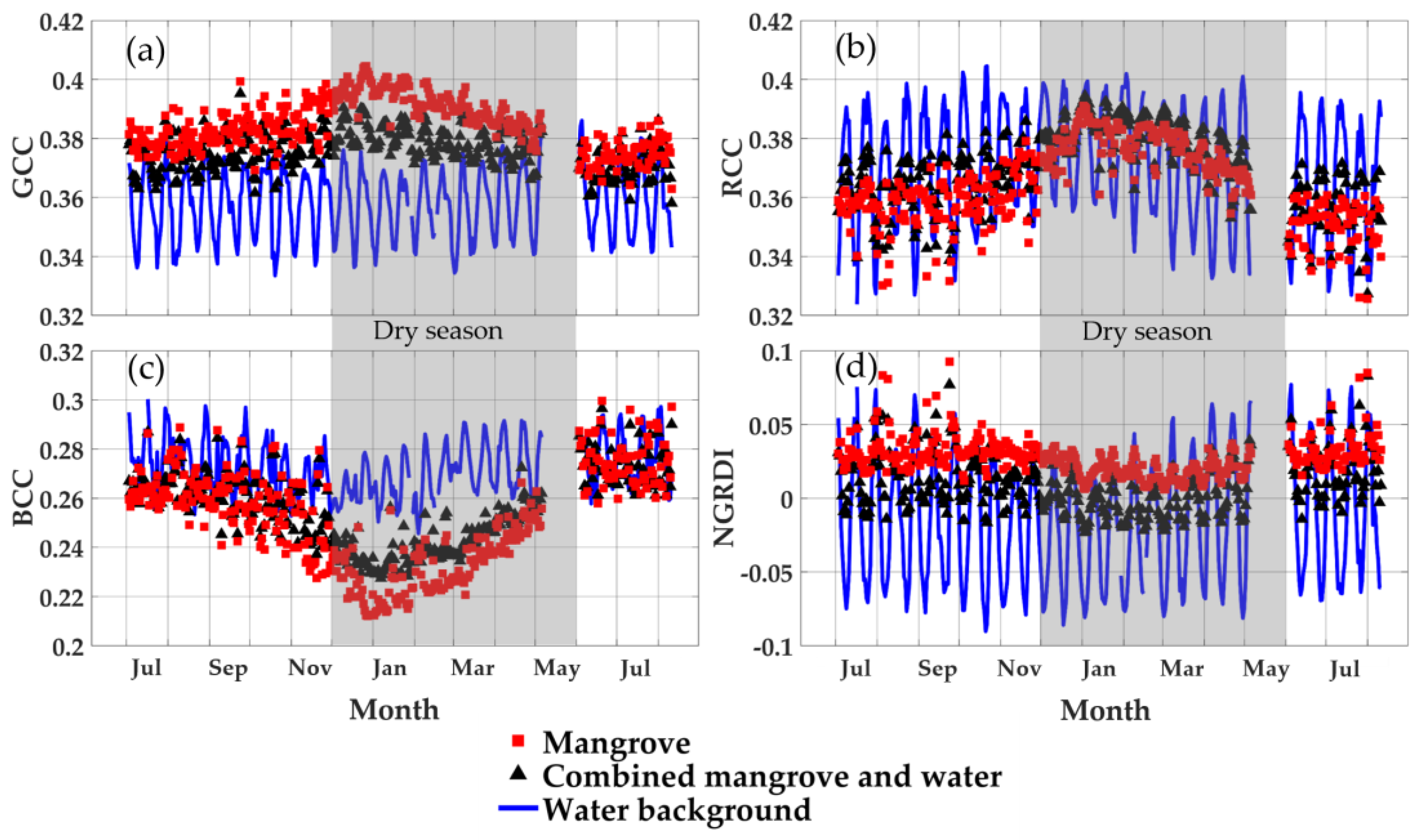
The diurnal data were composited into near-solar-noon daily values to generate seasonal RGB color index profiles of the mangrove forest, water background, and mangrove–water canopy (Figure 6). The mangrove forest GCC profile revealed maximum greenness values in the early dry season (January) and minimum values during the wet seasonal period (July–September) (Figure 6a). The combined mangrove–water canopy resulted in a similar but lower greenness profile that still peaked in the early dry season. However, the water-induced decrease was stronger in the dry season than in the wet season due to the greater occurrences of shallow, mud, and exposed soil backgrounds. The water background GCC values did not show clear seasonality, but instead exhibited strong periodicity of a 2-week frequency, apparently related to the lunar tidal cycles that occur twice per month. This periodicity can also be seen to a lesser extent in the mangrove forest and mangrove–water canopy GCC profiles (Figure 6a). These show GCC values to be positively related with the water level. In the wet season, the GCC signals from the mangrove–water canopy are nearly as high as that of the mangrove forest, suggesting the water GCC signals are as green as the mangrove forest GCC, possibly due to green scattering of sunlight from the mangrove forest onto the water surface.
The mangrove forest seasonal RCC profile behaved similarly to the GCC profile, but with greater seasonal contrast and no distinction between the mangrove forest and mangrove–water canopy ROIs (Figure 6b). This may be a result of the much greater fluctuations in the water background RCC values, which were well above and below the both mangrove profiles. Further, the water background RCC tidal periodicity was inverse to that of the GCC periodicity, i.e., RCC water tidal peaks aligned with GCC troughs (Figure 6a,b). This was consistent with the inverse relationship of the GCC with RCC found in the diurnal water background results (Figure 3c) and further indicates that RCC values were negatively related with the water level.
The mangrove forest seasonal BCC profile was inverse to the GCC and RCC seasonal profiles, with maximum BCC values in the wet season and minimum values in the dry season (Figure 6c). The mangrove–water canopy seasonal BCC profile was situated in-between that of the mangrove forest and water background, with water having distinctly higher BCC values year-round. Thus, similar to the seasonal GCC profile, the presence of water in the combined mangrove–water canopy ROI dampened the stronger seasonal contrast of the mangrove forest (Figure 6c). The water background BCC tidal periodicity was in phase with that of the GCC and positively related to increasing water levels.
Overall, the mangrove forest and mangrove–water canopy NGRDI profiles were similar to the equivalent GCC profiles, with the water NGRDI values being the lowest and mangrove forest NGRDI values being the highest (Figure 6d). However, their NGRDI seasonal profiles were lower in the dry season and higher in the wet season (Figure 6d), which was out of phase with the GCC profiles, although both were greenness indices. The seasonal difference between the mangrove and mangrove–water canopy was greatest in the wet season and lowest in the dry season, also out of phase with GCC profiles, which showed the largest differences in the dry season.
The NGRDI values are functionally related to the ratio of GCC to RCC, and one can see from Figure 6a,b that the ratio between GCC and RCC for the mangrove forest is greater in the wet season (0.385/0.36 = 1.07) than in the dry season (0.395/0.38 = 1.04), hence yielding higher NDGRI values in the wet season (0.034) than in the dry season (0.020). Seasonally, there is also an increase in the water background RCC in the dry season due to the lower water levels and exposure of mud and soil. This results in mangrove–water canopy RCC values being higher than RCC values for the mangrove forest in the dry season. The water background NGRDI tidal periodicity was in phase with that of GCC and BCC, and hence was positively related to increasing water levels.
3.5. Mangrove Forest Greenness Phenology
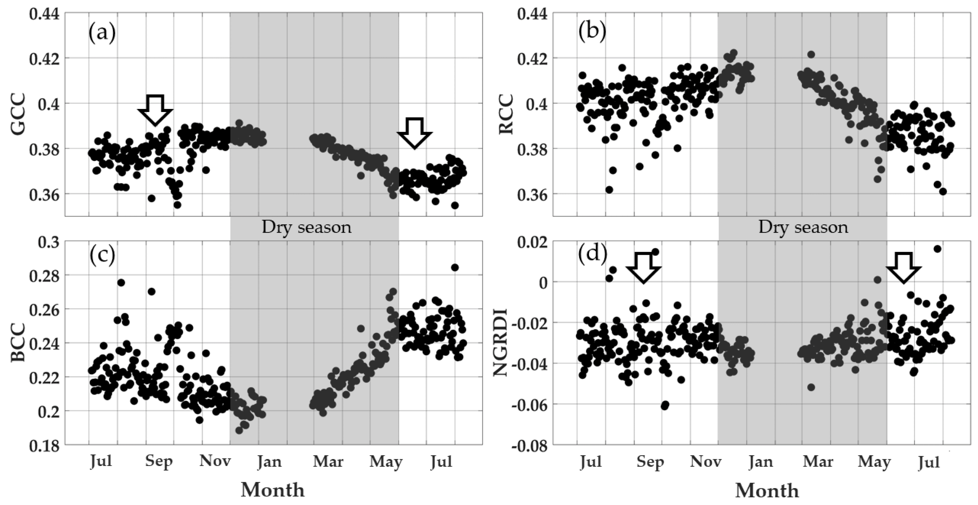
To confirm the out-of-phase mangrove phenology GCC and NGRDI profiles, we examined the corresponding profiles with the north-facing phenocam-1, which imaged a higher elevation portion of the mangrove forest (Figure 2 and Figure 7). The phenocam-1 mangrove forest seasonal RGB color index profiles resembled the phenocam-2 mangrove forest profiles (Figure 6), but with lower seasonal GCC and NGRDI values. Both phenocams showed mangrove forest profiles with similar phenology peak timings in the early part of the dry season around January, and phenological growth cycle commencing in the middle of the wet season, around June–July. The slightly lower values for the north-facing phenocam-2 were most likely a result of the absence of the strong backscattering signals seen in the west-facing phenocam-2 images. Both phenocams also exhibited similar RCC and BCC seasonal patterns. As with phenocam-2, the seasonal NGRDI greenness profile peaked in the wet season and was minimal in the dry season, remaining out of phase with GCC seasonal patterns. Whereas absolute NGRDI values were positive in phenocam-2 data, they were negative in phenocam-1 results (Figure 6 and Figure 7) as a consequence of the stronger backscattering signals in phenocam-2.
3.6. New Green Leaf Phenology
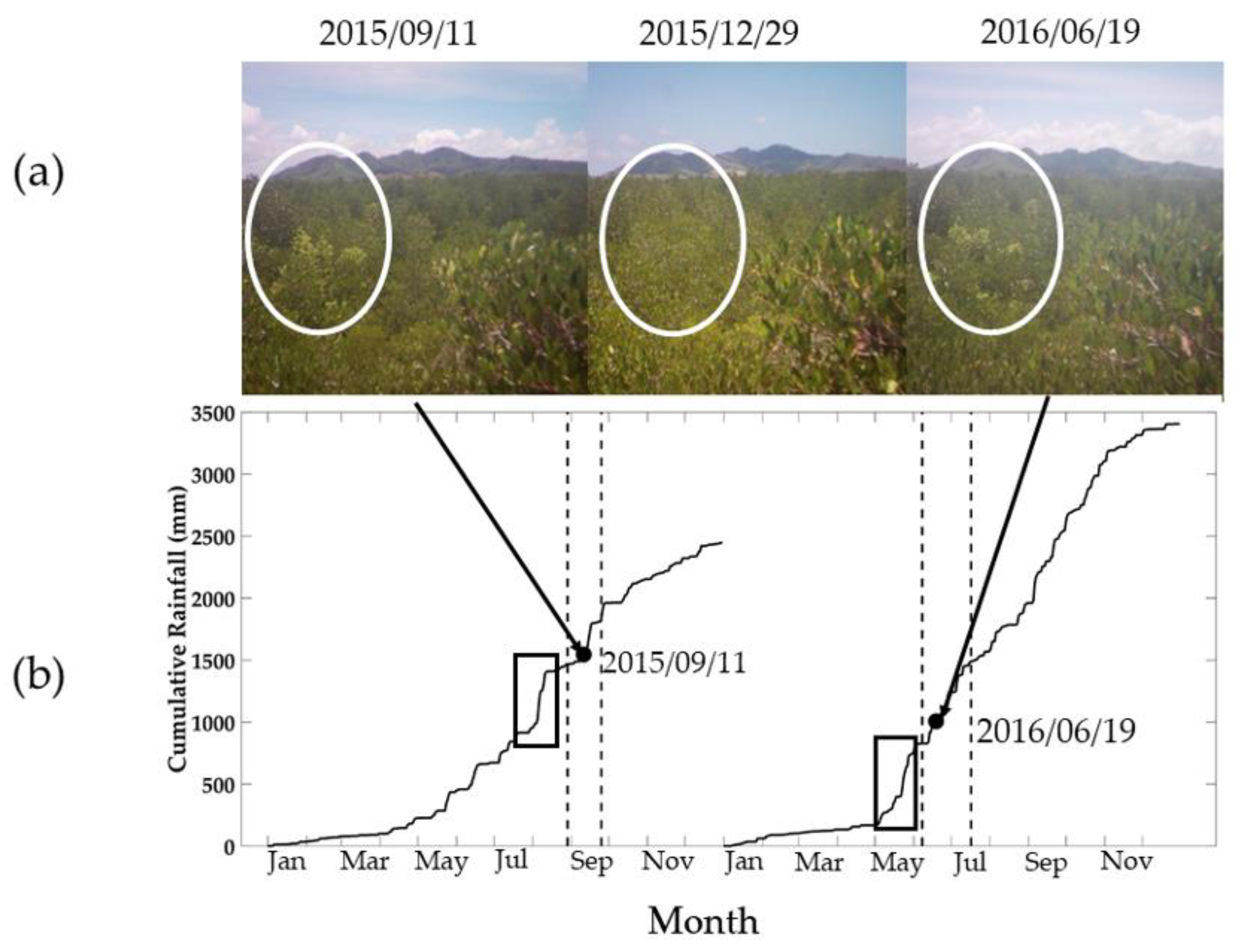
The appearance and timing of the mangrove leaf flushing was captured by phenocam-1 during September 2015 and June 2016 (Figure 8). The new leaf growth was observed shortly after periods of high cumulative rainfall (rectangle shapes in Figure 8b) for both seasons—the first season was in August 2015 and the second season was in May 2016. The new leaf growth started in September 2015, so the maximum greenness values were also observed in December or January of the dry season. The appearance of new leaves can be linked to the observed seasonality of the GCC values shown in Figure 7, with the new leaves appearing in September 2015 and June 2016 (Figure 8a), respectively.
3.7. Seasonal Relationships of RGB Color Indices with Water Level
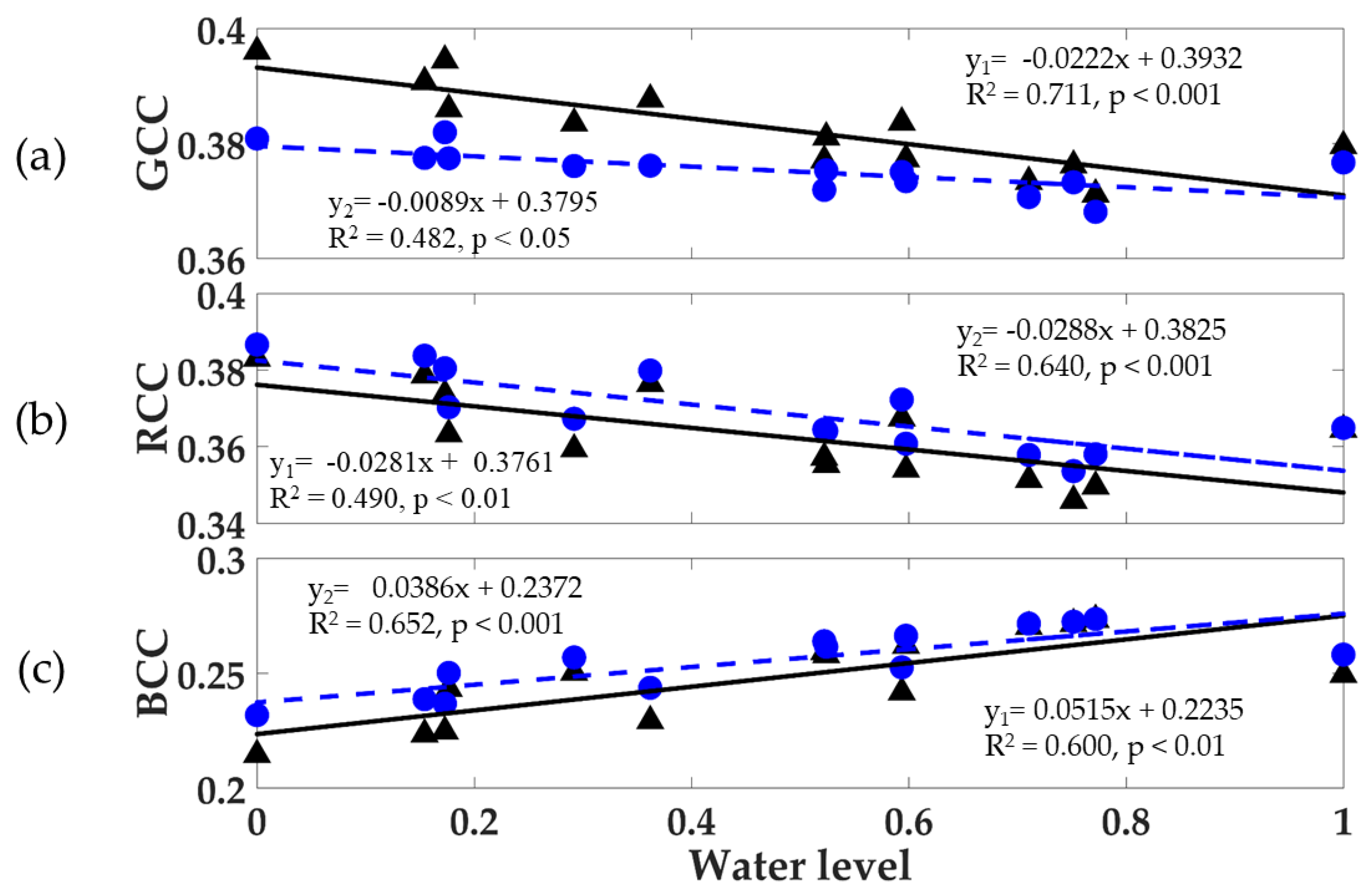
The seasonal relationships of GCC, RCC, and BCC values with the normalized water level are shown in Figure 9 for the mangrove forest and mangrove–water canopy ROIs from phenocam-2. Mangrove forest GCC values showed strong negative relationships with the water level (R2 = 0.711, p < 0.001, Figure 9a), reflecting the dry season peak activity in greenness found in both phenocam images (Figure 6 and Figure 7). This negative relationship was dampened and deteriorated (R2 = 0.482, p < 0.05) when the water background signal was included (mangrove–water canopy), since GCC values of the water were strongly positive correlated with the water level (Figure 3c, Table 2), hence counteracting and weakening the negative relationship with the mangrove forest. The decrease in GCC values caused by the water background was strongest at the lower water levels found in the dry season, where more sediment, mud, and soil are present, while there was no decrease in GCC values at the higher water levels, as both relationships converge.
The mangrove forest relationship with the water level would be an indirect, non-causal one, a consequence of peak mangrove greenness occurring in the dry season when water levels were at their lowest, while wet season GCC values were minimal when water levels were at their highest. Furthermore, daily water tidal levels greatly exceed water level differences between dry and wet seasons. The water level influences on mangrove forest phenocam indices can be evaluated by comparing the water level relationships of the combined mangrove–water canopy with the mangrove forest only. In the dry season, the presence of the water background exerted its greatest negative influence on GCC values, a result of the greater presence of mud, soil, and sediment exposure (Figure 9a). Thus, the mangrove forest phenology contrast between dry and wet seasons was considerably dampened by the presence of the water background GCC signal in the combined ROI.
The mangrove forest RCC values were also negatively correlated with the water level (R2 = 0.490, p < 0.01) and this relationship became stronger (R2 = 0.640, p < 0.001) with the presence of water in the mangrove–water canopy (Figure 9b). The RCC values of the mangrove–water canopy were higher than those from the mangrove forest. The lower water levels in the dry season contributed to the positive RCC signals due to the presence of muddy waters and exposed soil. On the other hand, the mangrove forest BCC values showed a positive relationship with the water level (R2 = 0.600, p < 0.01) and the inclusion of the water background with the mangrove forest increased the BCC values and strengthened the BCC relationships (R2 = 0.652, p < 0.001) with the water level.
4. Discussion
The two in situ phenocams were found to provide valuable information on the phenology of mangrove forests and offer strong monitoring capabilities of the mangrove–water background canopy at very fine temporal resolutions. As shown in this study, phenocams can be readily deployed in many different locations with minimal resources and their imagery can be spatially segmented into distinct regions of interest (ROIs) to evaluate the green leaf and water component signals of the highly dynamic mangrove–water canopy.
4.1. Mangrove Water Background
The phenocam color chromatic index measurements of the water background were dependent on the water depth, sediment content, exposed mud and soil, as well as scattering of radiation from the overlying mangrove trees. The diurnal phenocam index profiles at 30 min intervals captured the variations in tidal water depth, solar zenith angle, and their resulting interactions with the mangrove canopy scattering.
The tidal water influences on the color chromatic indices persisted at seasonal scales, exhibiting a 2-week periodicity aligning with the lunar tidal cycle. This periodicity was most strongly observed from the water background in all measured phenocam indices, which was further imparted onto the mangrove–water canopy ROI as well (Figure 6). Surprisingly, the lunar tide periodicity was also detected in the mangrove forest ROI despite the absence of water in the ROI. This could only be attributed to first order optical interactions between the water background and the surrounding, overlying mangrove forest. In the higher-elevation mangrove forest observed with phenocam-1, the tidal-water-induced periodicity was not apparent, particularly in the GCC signal (Figure 7a). Younes et al. [65] reported that red and green spectral signals are influenced by water depth and can influence vegetation fraction cover estimations.
The water influence in a mangrove–water canopy would be proportional to the relative fractions of water and mangrove forest present in the field of view (or ROI) of the phenocam. The relative proportions of water and mangrove forest in our mangrove–water ROI were approximately 1:5 (Figure 2c), or 20% water and 80% mangrove. The phenocam index values for varying mangrove–water proportions may be approximated with a linear mixture model, however there may also be non-linear optical interactions, such that the strongest water influence may occur at around 50% of the fractional amounts of mangrove and water, as has been reported in terrestrial canopy mixtures of soil and vegetation [66].
The upscaling and coupling of the in situ phenocam measures of mangrove forest phenology and water influences to satellite remote sensing would require knowledge of the sensor view angle and sun angle geometric orientations of the mangrove–water canopy. The oblique viewing phenocam results may not be easily interpolated to near-nadir canopy views. Additional information on the mangrove canopy structure (density, cover, and height), potentially through the use of LiDAR data, would enable a more complete understanding of the influence of shifting tidal waters and on broader scale satellite data signals.
4.2. Mangrove Forest Phenology
Our results show that equatorial mangrove green leaf seasonal growth, as measured by GCC values, was lowest in the wet season and highest (with GCC greenness peaks) in the dry season (January). This was true for both phenocams with different view orientations (Figure 6 and Figure 7). In the only other known phenocam study on mangrove forests, Xiang et al. [56] reported GCC values of a mangrove site in Hong Kong to be higher in summer (July) than in winter (February). This is opposite to our phenocam study, however Xiang et al. [56] only obtained 2 months of phenocam measurements and Hong Kong has marked differences in winter–summer maximum temperatures (18 °C to 31 °C, respectively) compared to our study site in Phuket, where temperatures are near-constant all year round. Our phenocam imagery further showed new mangrove leaf flushing in September 2015, after heavy rainfall activity and near the end of the monsoon season. After the start of the new leaf growth, the mangroves continually increased in greenness up to the early dry season in December–January, at which time conditions were suitable for the reproductive phenophase involving flowering, pollination, and eventual fruiting. This was similar to the reported values in prior field studies of the same mangrove species studied here, Rhizophora apiculata, in Phuket, Thailand [20], in which major flowering activity occurred between December to February, with the fruiting occurring in the wet season months of May and June. The production of Rhizophora mucronata flower buds in the lower rainfall dry season was also reported in Malaysia [67].
Various studies have also suggested that seasonal greenness measures of mangrove forests depend on leaf flushing and leaf development, as well as rates and periods of litter fall [32]. Pastor-Guzman et al. [32] found that the litter fall of mangroves in southeast Mexico showed higher rates during the ends of both the dry and wet seasons, while other tropical mangrove studies in India have reported maximum litter fall during the pre- and post-monsoon periods [22,68]. In our study, we lacked information on litter fall and could not assess its influence in the interpretation of the GCC mangrove phenology profiles. In a terrestrial broadleaf deciduous study using phenocams [44], the RCC index was found to be potentially useful for extracting leaf fall dates, because dried fallen leaves showed higher RCC values.
We encountered out-of-phase phenology profiles from two greenness measures used in our study, the GCC and NGRDI, with the out-of-phase phenologies observed in both phenocam-1 and phenocam-2. This could present ambiguous results in interpreting mangrove phenology with phenocams. The research by Pastor-Guzman et al. [32] reported that the dates of key mangrove phenological events were dependent on selecting the appropriate vegetation index. We found that overall, NGRDI values provided very little seasonal information with very low annual variation in values (Figure 6d and Figure 7d). Further, the NGRDI values dramatically changed from negative to positive values for phenocam-1 and phenocam-2, respectively, indicating high sensitivity to view orientation geometry. Lastly, the prior studies conducted in Thailand and Malaysia mangroves [20,67] support the new leaf growth patterns observed for GCC rather than the NRGDI patterns. Nevertheless, we suggest that the use of greenness and other optical indices in mangrove environments, which are often inundated with water, should be carefully evaluated.
4.3. Illumination
Our results revealed many of the intricacies involving optical interactions between solar radiation, mangrove vegetation, and adjacent and below-canopy standing water. We found significant illumination variations due to the sun angle and direct and diffuse sky conditions in our sub-daily, diurnal results, despite having normalized our phenocam color digital numbers (DNs) by the sum of the 3 bands to generate the color chromatic indices (Table 1). Sun angle variations had pronounced effects on the color index values associated with phenocam azimuthal view orientations. The west-facing phenocam field-of-view resulted in strong backscatter (sunlit) and forward scatter (shaded) canopy color index diurnal profiles. The GCC and RCC were sensitive to sunlight conditions, while the BCC was more sensitive to the canopy shadowing (Figure 3). The color index diurnal patterns were more pronounced in the dry season, when direct sunlight is more prevalent, and were less pronounced in the wet season, when ubiquitous clouds and diffuse sky conditions are more prevalent. In the case of the north-facing phenocam, sun angle illumination effects were not as pronounced,’ since the sunlit and shadow proportions of the mangrove canopy were equally present in the phenocam’s field-of-view. Xiang et al. [56] similarly reported illumination and shading as important factors influencing the quality of phenocam color indices. Due to the strong sun angle effects, we composited the 30-min, sub-daily phenocam data to daily values by restricting sun angle conditions to mid-day, near solar noon, from 10:00 to 14:00 (local time), and by selecting the 90th percentile. The observations near solar noon both reduced the sun angle effects and produced a more consistent daily phenology measure.
5. Conclusions
Mangrove phenology assessment based on digital repeat photography or phenocam imagery was analyzed in this study, with this approach found to have great potential for monitoring and evaluating mangrove phenology. The phenocams were able to extract reliable sub-daily, daily, and seasonal information about the status of the mangrove vegetation and below-canopy water properties, including the water color and relative water depth. The strong lunar tidal water periodicity was detectable with the phenocam color indices, both in the diurnal and seasonal profiles, and not only in the water ROI, but also in the mangrove–water canopy ROI profile and the mangrove forest ROI phenology profile.
The phenocam results were sensitive to illumination and sun angle geometric orientations (solar zenith and azimuth angles). Our study, involving north- and west-facing phenocams, provides valuable information for more effective deployment of future phenocams with respect to their orientation and field of view to capture water and mangrove dynamics. The upscaling and integration of the phenocam-acquired information on water influences and mangrove forest phenology to satellite remote sensing will require knowledge and standardization of the sensor view and sun angle geometric properties of the mangrove–water canopy between the phenocam and satellite sensor. This will be crucial in order to effectively link high-precision phenocam data to longer-term satellite time series data for climate change studies.
We also found that phenological events such as leaf flushing could be identified. In our study site, we found that the growth phenology of the mangroves starts after the monsoon season and continues developing through to the end of the dry season, before decreasing in the wet season and repeating another growth cycle after the next monsoon period. Rainfall and water level are the major factors controlling the mangrove phenology, although rainfall was out of phase with mangrove phenology in the sense that the maximum mangrove activity was found to occur in the dry season, when maximum sunlight was available for photosynthesis. Given that we used low-end phenocams, we would expect that with new advances in time lapse cameras, with better optics and pixel resolutions, that high-precision mangrove phenology will further evolve and improve.
Due to the crucial role of mangrove forests in mitigating global warming, in situ phenocam measurements can provide valuable phenological information to achieve a better understanding of how mangroves may counter and mitigate climate change. In addition, the detection of mangrove phenology at the species level by digital repeat photography will better link to mangrove relationships with climate and environment drivers, and thus enable more sustainable conservation practices for mangrove forests in the future.
Author Contributions
A.H., W.K., and V.S. designed the research. V.S., W.K., A.H., and R.J.R. contributed to the writing and commented on the manuscript. All authors have read and agreed to the published version of the manuscript.
Funding
The study was jointly financed by Andaman Environment and Natural Disaster (ANED) research center and by the Faculty of Technology and Environment, Prince of Songkla University.
Acknowledgments
The authors would like to acknowledge the Faculty of Technology and Environment, Prince of Songkla University, Phuket Campus, Thailand, for providing financial support. The data used in this study were acquired as part of the mission of NASA’s Earth Science Division and archived and distributed by the Goddard Earth Sciences (GES) Data and Information Services Center (DISC), Hydrographics Department, Royal Thai Navy.
Conflicts of Interest
The authors declare no conflict of interest.
References
- Walker, J.; de Beurs, K.; Wynne, R.H. Phenological response of an Arizona dryland forest to short-term climatic extremes. Remote Sens. 2015, 7, 10832–10855. [Google Scholar] [CrossRef] [Green Version]
- Ma, X.; Huete, A.; Moran, S.; Ponce-Campos, G.; Eamus, D. Abrupt shifts in phenology and vegetation. J. Geophys. Res. Biogeosci. 2015, 120, 1–17. [Google Scholar] [CrossRef]
- Moore, C.E.; Brown, T.; Keenan, T.F.; Duursma, R.A.; Van Dijk, A.I.J.M.; Beringer, J.; Culvenor, D.; Evans, B.; Huete, A.; Hutley, L.B.; et al. Reviews and syntheses: Australian vegetation phenology: New insights from satellite remote sensing and digital repeat photography. Biogeosciences 2016, 13, 5085–5102. [Google Scholar] [CrossRef] [Green Version]
- Jeong, S.-J.; Ho, C.-H.; Gim, H.-J.; Brown, M.E. Phenology shifts at start vs. end of growing season in temperate vegetation over the Northern Hemisphere for the period 1982–2008. Glob. Chang. Biol. 2011, 17, 2385–2399. [Google Scholar] [CrossRef]
- Alongi, D.M.; Mukhopadhyay, S.K. Contribution of mangroves to coastal carbon cycling in low latitude seas. Agric. For. Meteorol. 2015, 213, 266–272. [Google Scholar] [CrossRef]
- Hogarth, P.J. The Biology of Mangroves and Seagrasses; Oxford University Press: Oxford, UK, 2007. [Google Scholar]
- Tue, N.T.; Dung, L.V.; Nhuan, M.T.; Omori, K. Carbon storage of a tropical mangrove forest in Mui Ca Mau National Park, Vietnam. Catena 2014, 121, 119–126. [Google Scholar] [CrossRef]
- Liu, H.; Ren, H.; Hui, D.; Wang, W.; Liao, B.; Cao, Q. Carbon stocks and potential carbon storage in the mangrove forests of China. J. Environ. Manag. 2014, 133, 86–93. [Google Scholar] [CrossRef]
- Wang, M.; Zhang, J.; Tu, Z.; Gao, X.; Wang, W. Maintenance of estuarine water quality by mangroves occurs during flood periods: A case study of a subtropical mangrove wetland. Mar. Pollut. Bull. 2010, 60, 2154–2160. [Google Scholar] [CrossRef]
- Mehlig, U. Phenology of the red mangrove, Rhizophora mangle L., in the Caete Estuary, Estuary, Para, equatorial Brazil. Aquat. Bot. 2006, 84, 158–164. [Google Scholar] [CrossRef]
- Kuenzer, C.; Bluemel, A.; Gebhardt, S.; Quoc, T.V.; Dech, S. Remote Sensing of Mangrove Ecosystems: A Review. Remote Sens. 2011, 3, 878–928. [Google Scholar] [CrossRef] [Green Version]
- Alatorre, L.C.; Sanchez-Carrillo, S.; Miramontes-Beltran, S.; Medina, R.J.; Torres-Olave, M.E.; Bravo, L.C.; Wiebe, L.C.; Granados, A.; Adams, D.K.; Sanchez, E.; et al. Temporal changes of NDVI for qualitative environmental assessment of mangroves: Shrimp farming impact on the health decline of the arid mangroves in the Gulf of California (1990–2010). J. Arid Environ. 2016, 125, 98–109. [Google Scholar] [CrossRef]
- Carter, H.; Schmidt, S.; Hirons, A. An International Assessment of Mangrove Management: Incorporation in Integrated Coastal Zone Management. Diversity 2015, 7, 74–104. [Google Scholar] [CrossRef]
- Jia, M.; Wang, Z.; Zhang, Y.; Ren, C.; Song, K. Landsat-Based Estimation of Mangrove Forest Loss and Restoration in Guangxi Province, China, Influenced by Human and Natural Factors. IEEE J. Sel. Top. Appl. Earth Obs. Remote Sens. 2015, 8, 311–323. [Google Scholar] [CrossRef]
- Duke, N.C. Phenological Trends with Latitude in the Mangrove Tree Avicennia Marina. J. Ecol. 1990, 78, 113–133. [Google Scholar] [CrossRef]
- Wang’ondu, V.W.; Kairo, J.G.; Kinyamario, J.I.; Mwaura, F.B.; Bosire, J.O.; Dahdouh-Guebas, F.; Koedam, N. Phenology of Avicennia marina (Forsk.) Vierh. in a Disjunctly-zoned Mangrove Stand in Kenya. West. Indian Ocean J. Mar. Sci. 2010, 9, 135–144. [Google Scholar]
- Rahman, M.M.; Islam, A.S. Phenophases of five mangrove species of the Sundarbans of Bangladesh. Int. J. Bus. Socia Sci. Res. 2015, 4, 77–82. [Google Scholar]
- Duke, N.C. Phenologies and Litter Fall of Two Mangrove Trees, Sonneratia alba Sm. And S. caseolaris (L.) Engl., and Their Putative Hybrid, S. × gulngai N.C. Duke. Aust. J. Bot. 1988, 36, 473–482. [Google Scholar] [CrossRef]
- Kamruzzaman, M.; Sharma, S.; Hagihara, A. Vegetative and reproductive phenology of the mangrove Kandelia obovata. Plant Species Biol. 2013, 28, 118–129. [Google Scholar] [CrossRef]
- Christensen, B.; Wium-Andersen, S. Seasonal growth of mangrove trees in southern Thailand. I. Phenology of RHIZOPHOZA APICULATA BL. Aquat. Bot. 1977, 3, 281–286. [Google Scholar] [CrossRef]
- Ellison, J.C.; Zouh, I. Vulnerability to Climate Change of Mangroves: Assessment from Cameroon, Central Africa. Biology 2012, 1, 617–638. [Google Scholar] [CrossRef] [Green Version]
- Wafar, S.; Untawale, A.G.; Wafar, M. Litter fall and energy flux in a mangrove ecosystem. Estuar. Coast. Shelf Sci. 1997, 44, 111–124. [Google Scholar] [CrossRef]
- Aksornkoae, S. Mangrove...Ecology and Management, 3rd ed.; Kasetsart University: Bangkok, Thailand, 1999. [Google Scholar]
- Metcalfe, K.N.; Franklin, D.C.; McGuinness, K.A. Mangrove litter fall: Extrapolation from traps to a large tropical macrotidal harbour. Estuar. Coast. Shelf Sci. 2011, 95, 245–252. [Google Scholar] [CrossRef]
- White, K.; Pontius, J.; Schaberg, P. Remote sensing of spring phenology in northeastern forests: A comparison of methods, field metrics and sources of uncertainty. Remote Sens. Environ. 2014, 148, 97–107. [Google Scholar] [CrossRef]
- Gonsamo, A.; Chen, J.M.; Price, D.T.; Kurz, W.A.; Wu, C. Land surface phenology from optical satellite measurement and CO 2 eddy covariance technique. J. Geophys. Res. Biogeosci. 2012, 117, 1–18. [Google Scholar] [CrossRef]
- Kariyeva, J.; Leeuwen, W.J.D. Van Environmental Drivers of NDVI-Based Vegetation Phenology in Central Asia. Remote Sens. 2011, 3, 203–246. [Google Scholar] [CrossRef] [Green Version]
- Zhang, X.; Friedl, M.A.; Schaaf, C.B. Global vegetation phenology from Moderate Resolution Imaging Spectroradiometer (MODIS): Evaluation of global patterns and comparison with in situ measurements. J. Geophys. Res. Biogeosci. 2006, 111, 1–14. [Google Scholar] [CrossRef]
- Jones, M.O.; Jones, L.A.; Kimball, J.S.; McDonald, K.C. Satellite passive microwave remote sensing for monitoring global land surface phenology. Remote Sens. Environ. 2011, 115, 1102–1114. [Google Scholar] [CrossRef]
- Clinton, N.; Yu, L.; Fu, H.; He, C.; Gong, P. Global-scale associations of vegetation phenology with rainfall and temperature at a high spatio-temporal resolution. Remote Sens. 2014, 6, 7320–7338. [Google Scholar] [CrossRef] [Green Version]
- Ide, R.; Oguma, H. Use of digital cameras for phenological observations. Ecol. Inform. 2010, 5, 339–347. [Google Scholar] [CrossRef]
- Pastor-Guzman, J.; Dash, J.; Atkinson, P.M. Remote sensing of mangrove forest phenology and its environmental drivers. Remote Sens. Environ. 2018, 205, 71–84. [Google Scholar] [CrossRef] [Green Version]
- Songsom, V.; Koedsin, W.; Ritchie, R.J.; Huete, A. Mangrove phenology and environmental drivers derived from remote sensing in Southern Thailand. Remote Sens. 2019, 11, 955. [Google Scholar] [CrossRef] [Green Version]
- Richardson, A.D.; Jenkins, J.P.; Braswell, B.H.; Hollinger, D.Y.; Ollinger, S.V.; Smith, M.L. Use of digital webcam images to track spring green-up in a deciduous broadleaf forest. Oecologia 2007, 152, 323–334. [Google Scholar] [CrossRef] [PubMed]
- Nagai, S.; Ichie, T.; Yoneyama, A.; Kobayashi, H.; Inoue, T.; Ishii, R.; Suzuki, R.; Itioka, T. Usability of time-lapse digital camera images to detect characteristics of tree phenology in a tropical rainforest. Ecol. Inform. 2016, 32, 91–106. [Google Scholar] [CrossRef]
- Sonnentag, O.; Hufkens, K.; Teshera-Sterne, C.; Young, A.M.; Friedl, M.; Braswell, B.H.; Milliman, T.; O’Keefe, J.; Richardson, A.D. Digital repeat photography for phenological research in forest ecosystems. Agric. For. Meteorol. 2012, 152, 159–177. [Google Scholar] [CrossRef]
- Younes Cárdenas, N.; Joyce, K.E.; Maier, S.W. Monitoring mangrove forests: Are we taking full advantage of technology? Int. J. Appl. Earth Obs. Geoinf. 2017, 63, 1–14. [Google Scholar] [CrossRef] [Green Version]
- Liu, Y.; Hill, M.J.; Zhang, X.; Wang, Z.; Richardson, A.D.; Hufkens, K.; Filippa, G.; Baldocchi, D.D.; Ma, S.; Verfaillie, J.; et al. Using data from Landsat, MODIS, VIIRS and PhenoCams to monitor the phenology of California oak / grass savanna and open grassland across spatial scales. Agric. For. Meteorol. 2017, 237–238, 311–325. [Google Scholar] [CrossRef]
- Baumann, M.; Ozdogan, M.; Richardson, A.D.; Radeloff, V.C. Phenology from Landsat when data is scarce: Using MODIS and Dynamic Time-Warping to combine multi-year Landsat imagery to derive annual phenology curves. Int. J. Appl. Earth Obs. Geoinf. 2017, 54, 72–83. [Google Scholar] [CrossRef]
- Lopes, A.P.; Nelson, B.W.; Wu, J.; de Alencastro Graça, P.M.L.; Tavares, J.V.; Prohaska, N.; Martins, G.A.; Saleska, S.R. Leaf flush drives dry season green-up of the Central Amazon. Remote Sens. Environ. 2016, 182, 90–98. [Google Scholar] [CrossRef]
- Richardson, A.D.; Braswell, B.H.; Hollinger, D.Y.; Jenkins, J.P.; Ollinger, S.V. Near-surface remote sensing of spatial and temporal variation in canopy phenology. Ecol. Appl. 2009, 19, 1417–1428. [Google Scholar] [CrossRef]
- Richardson, A.D.; Hufkens, K.; Milliman, T.; Frolking, S. Intercomparison of phenological transition dates derived from the PhenoCam Dataset V1.0 and MODIS satellite remote sensing. Sci. Rep. 2018, 8, 1–12. [Google Scholar] [CrossRef] [Green Version]
- Motohka, T.; Nasahara, K.N.; Oguma, H.; Tsuchida, S. Applicability of Green-Red Vegetation Index for remote sensing of vegetation phenology. Remote Sens. 2010, 2, 2369–2387. [Google Scholar] [CrossRef] [Green Version]
- Klosterman, S.T.; Hufkens, K.; Gray, J.M.; Melaas, E.; Sonnentag, O.; Lavine, I.; Mitchell, L.; Norman, R.; Friedl, M.A.; Richardson, A.D. Evaluating remote sensing of deciduous forest phenology at multiple spatial scales using PhenoCam imagery. Biogeosciences 2014, 11, 4305–4320. [Google Scholar] [CrossRef] [Green Version]
- Crimmins, M.A.; Crimmins, T.M. Monitoring plant phenology using digital repeat photography. Environ. Manag. 2008, 41, 949–958. [Google Scholar] [CrossRef] [PubMed]
- Inoue, T.; Nagai, S.; Kobayashi, H.; Koizumi, H. Utilization of ground-based digital photography for the evaluation of seasonal changes in the aboveground green biomass and foliage phenology in a grassland ecosystem. Ecol. Inform. 2015, 25, 1–9. [Google Scholar] [CrossRef] [Green Version]
- Keenan, T.F.; Darby, B.; Felts, E.; Sonnentag, O.; Friedl, M.A.; Hufkens, K.; O’Keefe, J.; Klosterman, S.; Munger, J.W.; Toomey, M.; et al. Tracking forest phenology and seasonal physiology using digital repeat photography: A critical assessment. Ecol. Appl. 2014, 24, 1478–1489. [Google Scholar] [CrossRef] [Green Version]
- Ide, R.; Oguma, H. A cost-effective monitoring method using digital time-lapse cameras for detecting temporal and spatial variations of snowmelt and vegetation phenology in alpine ecosystems. Ecol. Inform. 2013, 16, 25–34. [Google Scholar] [CrossRef]
- Migliavacca, M.; Galvagno, M.; Cremonese, E.; Rossini, M.; Meroni, M.; Sonnentag, O.; Cogliati, S.; Manca, G.; Diotri, F.; Busetto, L.; et al. Using digital repeat photography and eddy covariance data to model grassland phenology and photosynthetic CO2 uptake. Agric. For. Meteorol. 2011, 151, 1325–1337. [Google Scholar] [CrossRef]
- Toomey, M.; Friedl, M.A.; Frolking, S.; Hufkens, K.; Klosterman, S.; Sonnentag, O.; Baldocchi, D.D.; Bernacchi, C.J.; Biraud, S.C.; Bohrer, G.; et al. Greenness indices from digital cameras predict the timing and seasonal dynamics of canopy-scale photosynthesis. Ecol. Appl. 2015, 25, 99–115. [Google Scholar] [CrossRef] [Green Version]
- Zhang, X.; Jayavelu, S.; Liu, L.; Friedl, M.A.; Henebry, G.M.; Liu, Y.; Schaaf, C.B.; Richardson, A.D.; Gray, J. Evaluation of land surface phenology from VIIRS data using time series of PhenoCam imagery. Agric. For. Meteorol. 2018, 256–257, 137–149. [Google Scholar] [CrossRef]
- Nagai, S.; Inoue, T.; Ohtsuka, T.; Yoshitake, S.; Nasahara, K.N.; Saitoh, T.M. Uncertainties involved in leaf fall phenology detected by digital camera. Ecol. Inform. 2015, 30, 124–132. [Google Scholar] [CrossRef]
- Wingate, L.; Ogeé, J.; Cremonese, E.; Filippa, G.; Mizunuma, T.; Migliavacca, M.; Moisy, C.; Wilkinson, M.; Moureaux, C.; Wohlfahrt, G.; et al. Interpreting canopy development and physiology using a European phenology camera network at flux sites. Biogeosciences 2015, 12, 5995–6015. [Google Scholar] [CrossRef] [Green Version]
- Hufkens, K.; Friedl, M.; Sonnentag, O.; Braswell, B.H.; Milliman, T.; Richardson, A.D. Linking near-surface and satellite remote sensing measurements of deciduous broadleaf forest phenology. Remote Sens. Environ. 2012, 117, 307–321. [Google Scholar] [CrossRef]
- Zhao, J.; Zhang, Y.; Tan, Z.; Song, Q.; Liang, N. Using digital cameras for comparative phenological monitoring in an evergreen broad-leaved forest and a seasonal rain forest. Ecol. Inform. 2012, 10, 65–72. [Google Scholar] [CrossRef]
- Xiang, Q.; Zhou, Y.; Liu, J. Monitoring mangrove phenology using camera images. IOP Conf. Ser. Earth Environ. Sci. 2020, 432. [Google Scholar] [CrossRef]
- Suepa, T.; Qi, J.; Lawawirojwong, S.; Messina, J.P. Understanding spatio-temporal variation of vegetation phenology and rainfall seasonality in the monsoon Southeast Asia. Environ. Res. 2016, 147, 621–629. [Google Scholar] [CrossRef] [Green Version]
- Krauss, K.W.; Mckee, K.L.; Lovelock, C.E.; Cahoon, D.R.; Saintilan, N.; Reef, R.; Chen, L. How mangrove forests adjust to rising sea level. New Phytol. 2014, 202, 19–34. [Google Scholar] [CrossRef] [Green Version]
- Asbridge, E.; Lucas, R.; Ticehurst, C.; Bunting, P. Mangrove response to environmental change in Australia’s Gulf of Carpentaria. Ecol. Evol. 2016, 6, 3523–3539. [Google Scholar] [CrossRef] [Green Version]
- Peter, J.S.; Hogland, J.; Hebblewhite, M.; Hurley, M.A.; Hupp, N.; Proffitt, K. Linking phenological indices from digital cameras in Idaho and Montana to MODIS NDVI. Remote Sens. 2018, 10, 1612. [Google Scholar] [CrossRef] [Green Version]
- Hunt, E.R., Jr.; Cavigelli, M.; Daughtry, C.S.T.; Mcmurtrey, J.; Walthall, C.L. Evaluation of Digital Photography from Model Aircraft for Remote Sensing of Crop Biomass and Nitrogen Status. Precis. Agric. 2005, 6, 359–378. [Google Scholar] [CrossRef]
- Adamsen, F.J.; Pinter, P.J.; Barnes, E.M.; LaMorte, R.L.; Wall, G.W.; Leavitt, S.W.; Kimball, B.A. Measuring wheat senescence with a digital camera. Crop. Sci. 1999, 39, 719–724. [Google Scholar] [CrossRef]
- Tucker, C.J. Red and photographic infrared linear combinations for monitoring vegetation. Remote Sens. Environ. 1979, 8, 127. [Google Scholar] [CrossRef] [Green Version]
- Jannoura, R.; Brinkmann, K.; Uteau, D.; Bruns, C.; Joergensen, R.G. Monitoring of crop biomass using true color aerial photographs taken from a remote controlled hexacopter. Biosyst. Eng. 2015, 129, 341–351. [Google Scholar] [CrossRef]
- Younes, N.; Joyce, K.E.; Northfield, T.D.; Maier, S.W. The effects of water depth on estimating Fractional Vegetation Cover in mangrove forests. Int. J. Appl. Earth Obs. Geoinf. 2019, 83, 101924. [Google Scholar] [CrossRef]
- Fensholt, R.; Sandholt, I.; Proud, S.R.; Stisen, S.; Rasmussen, M.O. Assessment of MODIS sun-sensor geometry variations effect on observed NDVI using MSG SEVIRI geostationary data. Int. J. Remote Sens. 2010, 31, 6163–6187. [Google Scholar] [CrossRef]
- Nordatul Akmar, Z.; Wan Juliana, W.A. Reproductive phenology of two rhizophora species in Sungai Pulai Forest Reserve, Johor, Malaysia. Malays. Appl. Biol. 2012, 41, 11–21. [Google Scholar]
- Rani, V.; Sreelekshmi, S.; Preethy, C.M.; BijoyNandan, S. Phenology and litterfall dynamics structuring Ecosystem productivity in a tropical mangrove stand on South West coast of India. Reg. Stud. Mar. Sci. 2016, 8, 400–407. [Google Scholar] [CrossRef]
Figure 1.
Location of study area. The green point is the mangrove forest tower located in Bangrong Bay, Phuket province, Thailand (8.052°N and 98.415°E).
Figure 1.
Location of study area. The green point is the mangrove forest tower located in Bangrong Bay, Phuket province, Thailand (8.052°N and 98.415°E).

Figure 2.
Fields of view and orientations of the two phenocams installed in the mangrove forest tower enclosure, which protected the phenocams. (a) The green square represents the top view of mangrove tower roof, with the viewing directions for (b) phenocam-1 (north facing) and (c) phenocam-2 (west facing) both showing the region of interest (ROI) of the mangrove forest area (ROI 1, white rectangle), as well as the combined mangrove–water canopy (ROI 2, black rectangle), the area where water level estimates were made (ROI 3), and the water background (ROI 4) from phenocam-2 only.

Figure 3.
Diurnal variations of the phenocam-2 RGB color indices (GCC, RCC, BCC, and NGRDI) over 4 seasonal periods of the year for (a) the mangrove forest (ROI 1), (b) combined mangrove-water canopy (ROI 2), and (c) water background (ROI 4). The diurnal profiles were measured at 30-min intervals and 3-day averages for each seasonal period (14–16 July 2015; 18–20 October 2015; 29–31 December 2015; 7–9 April 2016). The local time was GMT + 07 h.

Figure 4.
Diurnal hourly time lapse sequence of phenocam-2 images in the (a) wet season (July 15) and (b) dry season (December 30), displaying tidal cycles of changing water level and water color, as well as changing illumination conditions from backscatter (morning) to forward scatter (afternoon) solar angles and differences between diffuse radiation (wet season) and global radiation (dry season).

Figure 5.
Normalized water level estimates for the diurnal tidal cycles for 4 seasonal periods, as determined from phenocam-2, ROI 3.
Figure 5.
Normalized water level estimates for the diurnal tidal cycles for 4 seasonal periods, as determined from phenocam-2, ROI 3.

Figure 6.
Phenocam-2 RGB color index seasonal profiles of the mangrove forest (ROI 1), water (ROI 4), and combined mangrove–water canopy (ROI 2) from July 2015 to August 2016: (a) GCC, (b) RCC, (c) BCC, and (d) NRGDI (blank area in May 2016 is missing data due to phenocam malfunction).
Figure 6.
Phenocam-2 RGB color index seasonal profiles of the mangrove forest (ROI 1), water (ROI 4), and combined mangrove–water canopy (ROI 2) from July 2015 to August 2016: (a) GCC, (b) RCC, (c) BCC, and (d) NRGDI (blank area in May 2016 is missing data due to phenocam malfunction).

Figure 7.
Phenocam-1 RGB color index seasonal profiles of the mangrove forest (ROI 1) from July 2015 to August 2016: (a) GCC, (b) RCC, (c) BCC, and (d) NRGDI. Heavy rain from mid-September into October 2015 induced GCC and BCC data spikes. The blank area between January and March 2016 is missing data due to a phenocam malfunction. The arrows indicate new leaf events.

Figure 8.
The timing of the appearance of new leaves as assessed by visual observation of phenocam-1 images. The new leaf growth was observed on 11 September 2015 and 19 June 2016. (a) The white circles in the top of the canopy images show the new leaf growth. (b) Plot of the cumulative rainfall from January to December for 2015 and 2016, with the dashed lines showing the time interval of the new mangrove leaf appearance. The two rectangles indicate the periods of rapid rainfall accumulation. Sprouting of new leaves occurs about 2 weeks after a major wet event.

Figure 9.
The relationship between (a) GCC, (b) RCC, and (c) BCC seasonal values with the seasonal normalized water level for the mangrove forest (black triangle, y1 relationship) and mangrove-water canopy (blue dot, y2 relationship). The data were calculated monthly from July 2015 to August 2016.
Figure 9.
The relationship between (a) GCC, (b) RCC, and (c) BCC seasonal values with the seasonal normalized water level for the mangrove forest (black triangle, y1 relationship) and mangrove-water canopy (blue dot, y2 relationship). The data were calculated monthly from July 2015 to August 2016.


Table 1.
Red, green, blue chromatic coordinate indices (RCC, GCC, BCC, respectively) and normalized green–red difference index (NGRDI) greenness indices derived from the phenocam images. Note: DN = digital number; R, G, and B = red, green, and blue bands, respectively).
Table 1.
Red, green, blue chromatic coordinate indices (RCC, GCC, BCC, respectively) and normalized green–red difference index (NGRDI) greenness indices derived from the phenocam images. Note: DN = digital number; R, G, and B = red, green, and blue bands, respectively).
| Equation No. | Equations | Research Sources | Research Applied |
|---|---|---|---|
| (1) | . | [34,41] | [31,42,51,60] |
| (2) | . | [34,41] | [36] |
| (3) | . | [41] | [36] |
| (4) | . | [61,63] | [41,64] |
Table 2.
Correlations of diurnal RGB color indices with normalized water levels. Wet is the wet season (July, October) and dry is the dry season (December, April).
Table 2.
Correlations of diurnal RGB color indices with normalized water levels. Wet is the wet season (July, October) and dry is the dry season (December, April).
| Index | Mangrove Forest | Mangrove–Water Canopy | Water Background | ||||||
|---|---|---|---|---|---|---|---|---|---|
| All | Wet | Dry | All | Wet | Dry | All | Wet | Dry | |
| GCC | 0.364 * | 0.152 | 0.551 ** | 0.442 ** | 0.210 | 0.701 ** | 0.888 ** | 0.903 ** | 0.887 ** |
| RCC | 0.301 * | 0.137 | 0.420 * | 0.094 | 0.018 | 0.125 | −0.728 ** | −0.806 ** | −0.673 ** |
| BCC | −0.344 * | −0.151 | −0.495 * | −0.296 * | −0.147 | −0.415 * | 0.202 | 0.294 | 0.131 |
| NGRDI | −0.019 | 0.046 | −0.029 | 0.317 * | 0.223 | 0.432 * | 0.852 ** | 0.894 ** | 0.831 ** |
Note: ** p < 0.001, *p < 0.01.
Publisher’s Note: MDPI stays neutral with regard to jurisdictional claims in published maps and institutional affiliations. |
© 2021 by the authors. Licensee MDPI, Basel, Switzerland. This article is an open access article distributed under the terms and conditions of the Creative Commons Attribution (CC BY) license (http://creativecommons.org/licenses/by/4.0/).
Share and Cite
MDPI and ACS Style
Songsom, V.; Koedsin, W.; Ritchie, R.J.; Huete, A. Mangrove Phenology and Water Influences Measured with Digital Repeat Photography. Remote Sens. 2021, 13, 307. https://0-doi-org.brum.beds.ac.uk/10.3390/rs13020307
AMA Style
Songsom V, Koedsin W, Ritchie RJ, Huete A. Mangrove Phenology and Water Influences Measured with Digital Repeat Photography. Remote Sensing. 2021; 13(2):307. https://0-doi-org.brum.beds.ac.uk/10.3390/rs13020307
Chicago/Turabian StyleSongsom, Veeranun, Werapong Koedsin, Raymond J. Ritchie, and Alfredo Huete. 2021. "Mangrove Phenology and Water Influences Measured with Digital Repeat Photography" Remote Sensing 13, no. 2: 307. https://0-doi-org.brum.beds.ac.uk/10.3390/rs13020307
Note that from the first issue of 2016, this journal uses article numbers instead of page numbers. See further details here.