Observations of Mesoscale Eddies in Satellite SSS and Inferred Eddy Salt Transport


1
International Pacific Research Center, School of Ocean and Earth Science and Technology, University of Hawaii, Honolulu, HI 96822, USA
2
Hawaii Institute of Geophysics and Planetology, School of Ocean and Earth Science and Technology, University of Hawaii, Honolulu, HI 96822, USA
*
Author to whom correspondence should be addressed.
Remote Sens. 2021, 13(2), 315; https://0-doi-org.brum.beds.ac.uk/10.3390/rs13020315
Submission received: 17 December 2020
/
Revised: 15 January 2021
/
Accepted: 15 January 2021
/
Published: 18 January 2021
(This article belongs to the Special Issue Moving Forward on Remote Sensing of Sea Surface Salinity)
Abstract
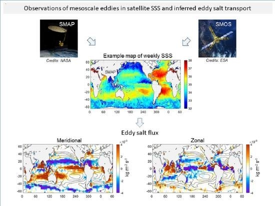
:Observations of sea surface salinity (SSS) from NASA’s Soil Moisture Active-Passive (SMAP) and ESA’s Soil Moisture and Ocean Salinity (SMOS) satellite missions are used to characterize and quantify the contribution of mesoscale eddies to the ocean transport of salt. Given large errors in satellite retrievals and, consequently, SSS maps, we evaluate two products from the two missions and also use two different methods to assess the eddy transport of salt. Comparing the two missions, we find that the estimates of the eddy transport of salt agree very well, particularly in the tropics and subtropics. The transport is divergent in the subtropical gyres (eddies pump salt out of the gyres) and convergent in the tropics. The estimates from the two satellites start to differ regionally at higher latitudes, particularly in the Southern Ocean and along the Antarctic Circumpolar Current (ACC), resulting, presumably, from a considerable increase in the level of noise in satellite retrievals (because of poor sensitivity of the satellite radiometer to SSS in cold water), or they can be due to insufficient spatial resolution. Overall, our study demonstrates that the possibility of characterizing and quantifying the eddy transport of salt in the ocean surface mixed layer can rely on the use of satellite observations of SSS. Yet, new technologies are required to improve the resolution capabilities of future satellite missions in order to observe mesoscale and sub-mesoscale variability, improve the signal-to-noise ratio, and extend these capabilities to the polar oceans.
1. Introduction
Sea surface salinity (SSS) is an essential climate variable that reflects changes in the marine hydrological cycle and plays an important role in ocean dynamics [1]. Over 80% of the Earth’s surface freshwater flux, precipitation (P) minus evaporation (E), occurs over the ocean’s surface [2,3], leaving an imprint on SSS. Therefore, changes in the SSS distribution can be used to monitor changes in the Earth’s water cycle [2,3]. Variations in SSS also affect the density of sea water, influencing the stability of the upper-ocean stratification and mixing [2]. This is particularly important at high latitudes, where salinity is a major factor controlling seawater density. For example, a complete shutdown of deep convection in the Labrador Sea is possible due to the increased freshening of the ocean surface layer linked to the accelerated melting of the Greenland ice sheet [4]. In the tropics, surface salinity can play a unique role in determining the depth of the surface mixed layer, indirectly affecting the air–sea exchanges of heat and momentum [5]. Therefore, knowledge of the SSS distribution is necessary for understanding the hydrological cycle, ocean circulation, and for monitoring changes in the ocean component of the Earth’s climate system. To this end, a better understanding of the physical processes governing the distribution of SSS is required.
The distribution of SSS is governed by a variety of physical processes varying over a broad range of spatial and temporal scales, and all require quantitative evaluation to connect variations in SSS to variations in the marine hydrological cycle [6,7]. Among these physical processes is horizontal advection by ocean currents and, in particular, by currents associated with mesoscale variability. Indeed, kinetic energy in the ocean surface layer is dominated by mesoscale variability or eddies [8,9]. Eddies are thought to play an important role in shaping the distribution of salt in the ocean [10], although it is not yet clear quantitatively what the overall role of the eddies is in the ocean salt budget, particularly in the surface mixed layer where the ocean interacts with the atmosphere [11]. Studies of mesoscale SSS variability are usually limited to relatively small geographic areas where high-resolution salinity observations exist [12], or they utilize outputs of ocean models [13]. However, the latter may have their own inadequacies, arising for example, from insufficient resolution and/or errors in the forcing fields [7,14]. For consistent description, observational estimates of the eddy fluxes are required [15].
Observations of ocean salinity have significantly been expanded in the last decade with the advent of satellite technology [16,17]. European Space Agency’s Soil Moisture and Ocean Salinity (SMOS) satellite was launched in November 2009 and since then has provided near-global observations of SSS with unprecedented spatial and temporal resolution. The Aquarius/SAC-D satellite, a collaborative mission between NASA and Argentina’s space agency, was launched in June 2011 and operated for 4 years, delivering high-quality salinity data, followed by continuous, high-resolution, near-global observations of SSS from NASA’s Soil Moisture Active-Passive (SMAP) satellite, which was launched in January 2015. More details on the technical characteristics of Aquarius/SAC-D, SMOS, and SMAP satellite missions can be found in, e.g., [16].
Satellite observations of SSS provide continuous time series with enhanced spatial and temporal resolution not available by other components of the global ocean observing system (GOOS). However, this is a new technology, and it is known that satellite-based observations of SSS are prone to significant errors. Typical errors in footprint measurements can be as large as 1 psu [18,19]. Errors are reduced to 0.2–0.3 psu in gridded SSS maps [19,20], but they are still quite large compared to the accuracy of in situ measurements, such as from Argo profiling floats. The errors are comparable to a typical eddy-induced SSS anomaly of O (0.1–0.3 psu) [11,21,22,23], and the signal-to-noise ratio for a mesoscale eddy signal appears to be low.
Despite these limitations, several studies have demonstrated the ability of satellite SSS measurements to observe mesoscale eddies [11,16,24]. For example, in [24], the observed patterns of eddy-induced SSS and sea surface height (SSH) anomalies were used to quantify the contribution of eddies to the ocean transport of salt in the subtropical North Atlantic. In another regional study, [25] used satellite SSS data to quantify meridional eddy salt transport in the three subtropical gyres in the Southern Hemisphere. Their results for the South Indian Ocean suggest that the eddy-induced salt flux can accomplish as much as 50% of the required divergence of salt out of the subtropical evaporative regime, perhaps explaining why the South Indian Ocean is the freshest among the three subtropical SSS maxima in the Southern Hemisphere. Yet, in spite of a few successful regional studies, it is still not completely clear as to what extent the new satellite-derived SSS data are suitable for studying the mesoscale signal [11].
The goal of this paper is twofold. First, we intend to characterize eddy salt fluxes in the ocean surface mixed layer globally using satellite observations of SSS. Second, we attempt to answer a question as to what extent such estimates are reliable enough to make quantitative conclusions, given the fact the satellite SSS data are of relatively short duration and also characterized by relatively large root-mean-square (RMS) errors, particularly at mesoscale resolution. To this end, we evaluate two products from two satellite missions, SMAP and SMOS. Although the two satellites use the same principles to retrieve SSS (the satellites provide measurements of the surface brightness temperature at L-band radiometric frequency), they differ significantly in the design, observation approach, and retrieval algorithms [18]. Therefore, the two satellite SSS datasets can be considered quasi-independent. Thus, comparing the two satellite missions may help establish confidence in our analysis and show if and where the satellite data are mature enough to provide reliable estimates of the eddy transport. We also evaluate two methods to estimate the eddy transport of salt. The first is indirect and is based on the so-called eddy composite analysis (e.g., [24]). The second is a traditional approach, which estimates the eddy flux as a covariance between eddy-induced velocity and SSS perturbations at a given geographical location [15]. This is also a novel element of our study. The rest of the paper is organized as follows. Section 2 describes the satellite data used in the study. In Section 3, we will look into how the two satellites “see” the mesoscale SSS signal using a representative example in the South Indian Ocean. Then, we will infer eddy fluxes of salt in the surface mixed layer globally using two satellite SSS datasets and also two different methods. To put our flux estimates into perspective, we will evaluate eddy salt flux divergence in each of the five subtropical gyres and compare it to the climatological mean surface freshwater flux (evaporation minus precipitation, E–P) to assess the role played by mesoscale eddies in balancing the E–P flux. A concluding discussion is in Section 4.
2. Data and Methods
2.1. Data
Two satellite-based SSS datasets have been used in our study.
SMOS SSS data are debiased Level-3 version 4 maps generated by LOCEAN/ACRI-ST Expertise Center [20]. We use 9-day maps produced on a 25-km × 25-km grid with a temporal interval of 4 days. The dataset covers the period from January 2010 to September 2019. The maps are derived from SMOS SSS Level-2 (swath) data by temporally averaging pixel observations over a 9-day running Gaussian kernel and spatially averaging neighbor observations over a 30-km radius circle around each grid point. The estimated spatial resolution of this product is approximately 75 km [20].
SMAP SSS data used in this study are produced by a Remote Sensing System (RSS) and consist of gridded SSS fields obtained by the temporal averaging of geo-located SMAP SSS Level-2 data. We use 8-day Level-3 SSS maps produced on a regular 0.25°-latitude × 0.25°-longitude Earth grid created by averaging all valid Level-2 (swath) observations within each grid cell. The maps are produced daily by applying an 8-day running average that is centered on a particular day of the year. The dataset covers the period from April 2015 to the present. For consistency with SMOS data, we used maps with a 4-day temporal interval. The effective spatial resolution of this product is approximately 70 km. A detailed description of SMAP SSS data can be found in [26].
Additional observational datasets are used to assess the eddy transport of salt.
Sea-level anomaly (SLA) observations from satellite altimetry and the associated surface geostrophic velocity fields are provided by the Copernicus Marine Environment Monitoring Service (CMEMS). In our study, we use a multi-satellite version of the product. The dataset covers the period from 1993 to the present and consists of daily SLA and surface geostrophic velocity fields on a 0.25°-longitude × 0.25°-latitude grid.
To track the signal of individual eddies, we use the Mesoscale Eddy Trajectory Atlas version 2.0 (META v2.0, [27]). The dataset covers the period from 1993 to 2019 and consists of more than 350,000 trajectories of eddies detected and tracked in SLA maps using the methodology of [28]. For each eddy, the dataset includes coordinates of the eddy center, eddy amplitude, eddy radius scale, and the average radial speed.
2.2. Methods
To assess the transport properties of individual eddies, we performed the so-called eddy composite analysis. The eddy composite analysis consists of a few simple steps and involves averaging over all snapshots of a variable of interest (in our case SSS) around individual eddies (eddy “realizations”) identified in SLA maps. Specifically, we used weekly SSS fields sampled in 500-km by 500-km boxes around the eddy centers identified in the eddy dataset. In a given geographic area (bin), the averages included only eddies located inside the area’s boundaries. In addition, in order to isolate the eddy signal and remove large-scale variability, prior to the composite analysis, the SSS and SLA fields were high-pass filtered using a 2D Hanning filter of half-width of 6°.
Following the approach by [31] for the heat flux, the meridional transport of salt due to a composite eddy can be estimated as [24]
where is eddy meridional velocity, is eddy SSS anomaly, and is the mixed-layer depth (MLD, which can be estimated from regional climatology (e.g., [11]). The angular brackets denote composite averages. The integral in (1) is taken over the eddy “wavelength” to ensure that the mean mass transport across the eddy is zero [31]. Zonal transport can be estimated similarly.
The eddy transport of salt in the surface mixed layer can also be estimated in a traditional way by computing covariances between eddy-induced velocity and SSS perturbations at a given geographical location as , where and are eddy-induced fluctuations of surface velocity and SSS. In Section 3, we estimate the eddy-induced salt flux from a multi-year time series of SSS and SLA (geostrophic velocity). In this case, to separate the eddy signal from low-frequency variability (annual and longer time-scales), the analysis is made using decomposition in the frequency domain. Following the approach by [14] for the heat flux, the zonal and meridional components of the eddy salt flux can be determined as
where , and are Fourier transforms of the velocity and salinity time series, the asterisk denotes complex conjugate, and is frequency. The integration in (2) is over the frequency band [ ], which is associated with the eddy variability and is taken in our study to be time scales shorter than 6 months.
3. Results
3.1. Regional Example
As introduced above, two satellite-derived SSS datasets are used in this study, which are hereafter called SMOS and SMAP SSS for short. We select the overlapping period in the two datasets from April 2015 to May 2019 to perform a comparative analysis of mesoscale variability.
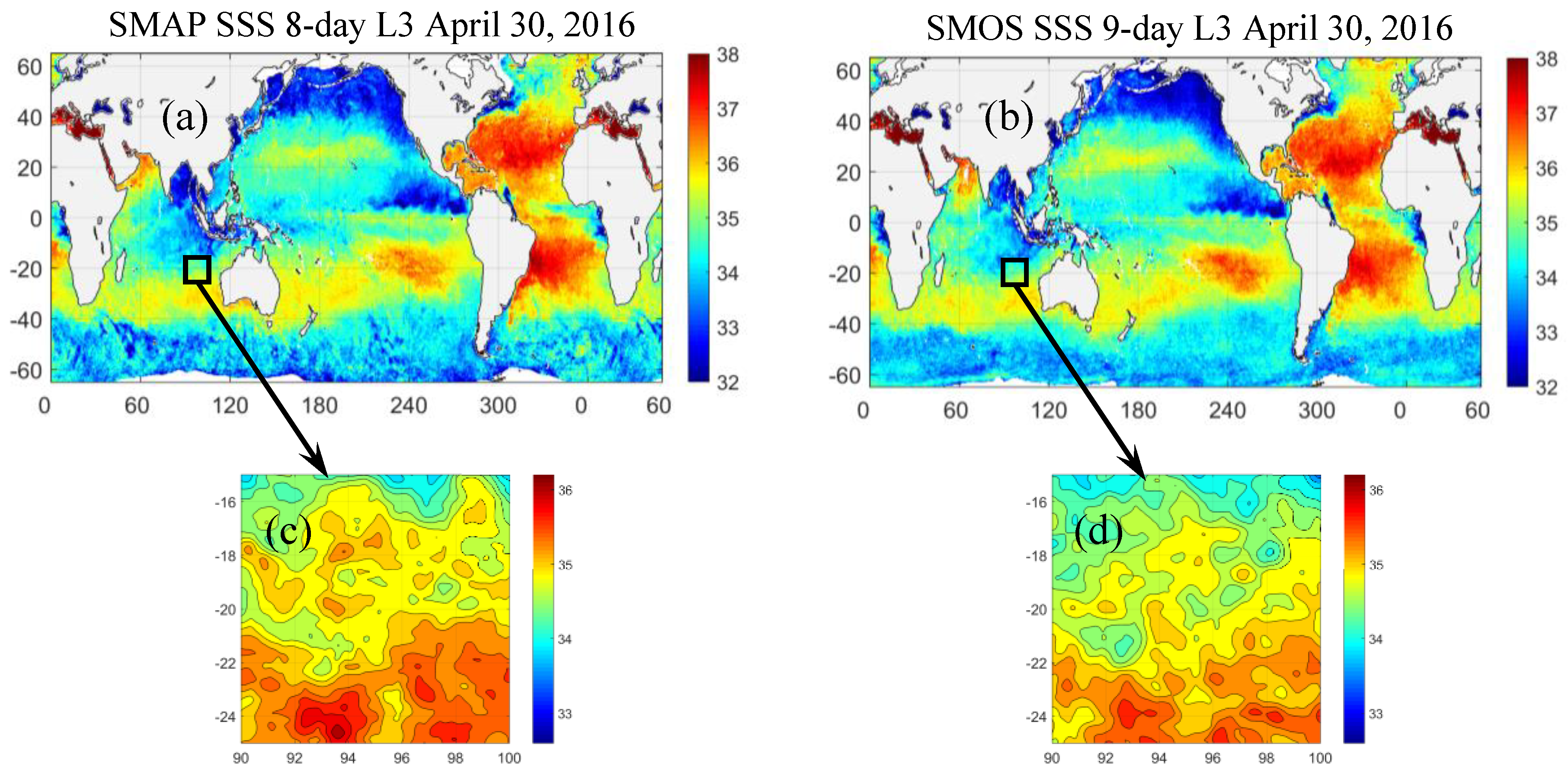
Figure 1 presents examples of the weekly maps from the two satellites. The maps are for the same week (9-day and 8-day running averages, to be more exact) and thus, technically, have to “see” the same structure. As expected, the two SSS fields demonstrate the same basin-scale structure. Surface salinity is higher in the subtropics (there are SSS maxima in all five subtropical oceans) and lower in the tropics and high latitudes. There are, practically, no differences between the maps at these scales. However, there are significant discrepancies at smaller scales and, in particular, at the mesoscale. To illustrate this, the inserts in Figure 1 show zooms on a 10°-longitude × 10°-latitude area in the South Indian Ocean. The mesoscale structures in these maps look quite different, and the differences can be as large as 0.2 psu.
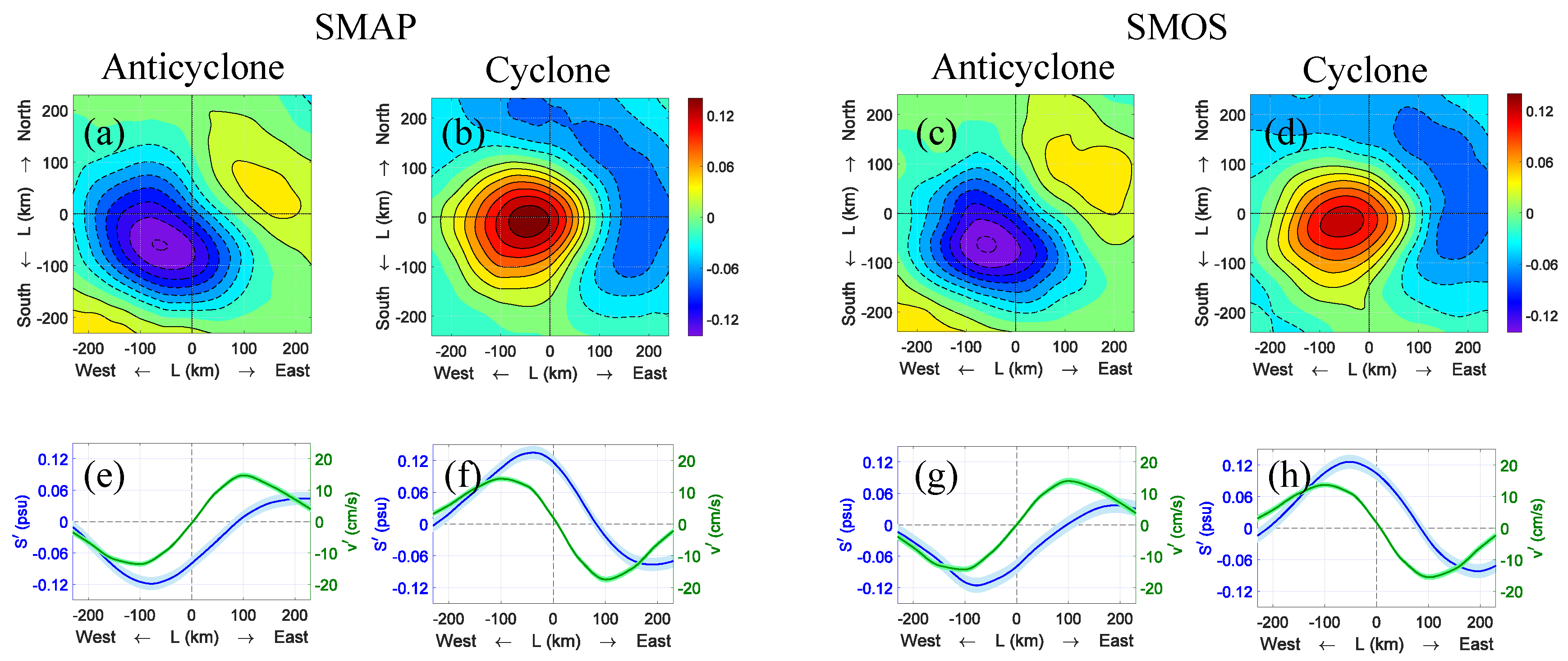
Such large discrepancies between the SSS maps in the mesoscale range raise a question as to what extent the satellite-derived SSS maps are suitable for mesoscale studies and, in particular, for estimating such a delicate matter as the eddy-induced transport of salt. This question would be in line with the analysis by [11], who argue that “one would first need to have much smaller error bars”. To address this question, let us first consider a regional example in the South Indian Ocean (SIO). The region is chosen somewhat arbitrarily; yet, it corresponds to a previous study [24], which first revealed the signature of mid-ocean mesoscale eddies in satellite SSS. Following [24], to suppress the noise, we average SSS maps in the reference frame co-moving with individual eddies (from the eddy dataset) and construct eddy composites. Over 268 cyclonic and 215 anticyclonic eddy realizations were found in the eddy dataset in the study region for the period from April 2015 to May 2019. Composite structures of eddy-induced SSS anomalies, corresponding to the average eddies, are shown in Figure 2, where we compare composite eddies in SMOS and SMAP observations, respectively. Remarkably, the two datasets result in virtually identical SSS anomaly patterns corresponding to an average eddy, despite the high level of noise and discrepancies in individual snapshots. By averaging over many eddy realizations, we have been able to average the noise out and infer only the essential, persistent structure of eddy-induced SSS anomalies. This example also illustrates that the noise in the maps in the mesoscale range is not correlated (particularly between the two satellites) and can effectively be suppressed by proper averaging. Finally, using Equation (1), we can estimate the meridional transport of salt associated with the composite eddies in Figure 2. An average anticyclonic (cyclonic) eddy identified in the study domain transports ≈ kg/s of salt northward in a 50-m surface mixed layer. Again, the estimates remarkably agree between the two satellite datasets.
It is worth reiterating that a net eddy flux of salt by an average eddy arises due to systematic phase differences between eddy-induced SLA and SSS perturbations such that the eddy velocity and SSS perturbations correlate over the eddy “wavelength” [32]. In particular, this is how westward-propagating eddies are able to provide meridional transport of salt. To illustrate this effect, Figure 2 (bottom panels) shows zonal sections across the composite eddies. The SSS anomaly (blue curves) is generally in phase with the eddy meridional velocity (green curves), producing in a positive correlation over the eddy length (; eddies pump salt northward). The standard error of each eddy composite is estimated from the standard deviation of the corresponding SSS anomaly and the number of eddy realizations used to compute the average. The standard error in all cases is quite small, smaller than 0.02 psu, showing that the eddy-induced SSS anomalies are well defined in the satellite SSS data, adding confidence to our estimates.
3.2. Eddy Salt Transport by Mean of Eddy Composite Analysis
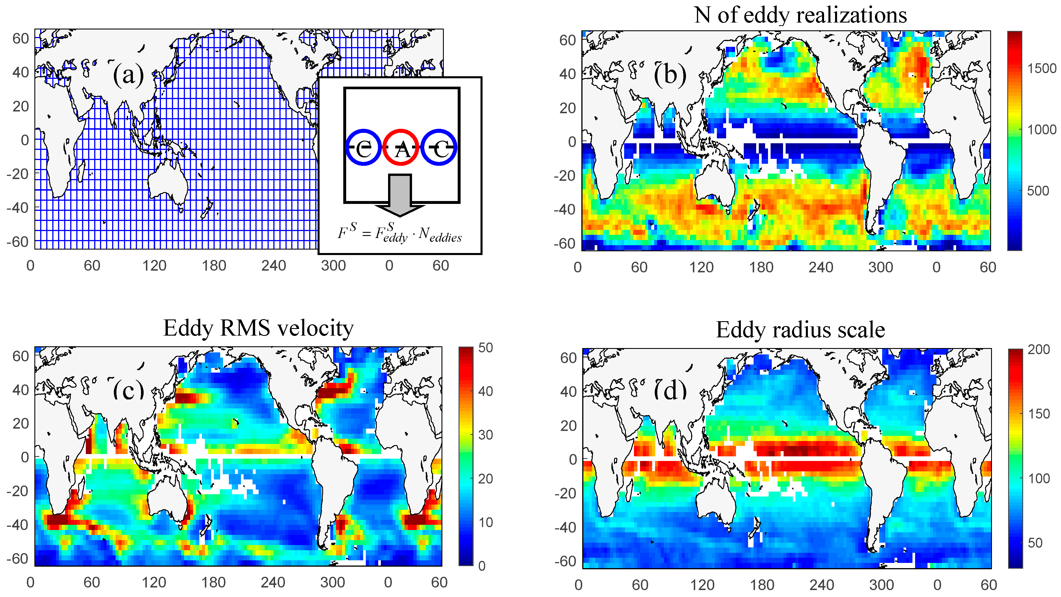
Using eddy composites reconstructed in different parts of the ocean, we can estimate the eddy transport of salt. Following the approach by [33], the ocean is presumed to be densely packed with mesoscale eddies. Therefore, a zonal or meridional section can be treated as a sequence of cyclonic and anticyclonic eddies (Figure 3a). In a limited geographic area (bin), eddies are assumed to be geometrically and dynamically similar such that their average effect can be represented by a “typical” (composite) eddy [34]. Then, the eddy flux across the section can be computed as the flux per a composite eddy multiplied by the number of eddies that can geometrically fit into the section.
To utilize this idea globally, we divide the ocean into 6°-longitude × 6°-latitude geographic bins. The bin size of 6° (≈600 km) is chosen because it corresponds to the average eddy propagation distance of 550 km derived from the satellite altimetry data [9] and thus seems to be optimal. Eddy composites are constructed in each geographic bin, and the eddy flux across the bin is estimated using the idea of the densely packed eddies as described above. A schematic illustration of the algorithm as well as maps of eddy properties relevant to our study is provided in Figure 3.
The distribution of the number of eddy realizations found in every 6° × 6° region over the 4-year period from April 2015 to May 2019 is shown in Figure 3b. In each bin, the number of eddy realizations is defined as the number of eddy centroids found in the bin divided by the number of SLA (SSS) maps used to cover a 28-day period. This way, the number of eddy realizations does not depend on whether daily or, e.g., weekly maps are used to identify eddies and construct eddy composites. The 28-day period is chosen somewhat arbitrarily; yet, it corresponds to the minimum lifetime of eddies in the eddy dataset and can be viewed as the Lagrangian decorrelation time scale. These numbers are also used to assess error bars in the eddy composite estimates. Figure 3b shows that a larger number of eddy realizations is typically observed in mid-latitudes; fewer eddies are found in the tropics. The latter can partially be attributed to the larger length scale of eddies in the tropics (Figure 3d), such as fewer eddies can simultaneously fit into a bin.
The map of eddy RMS velocity in Figure 3c shows that large-amplitude eddies with the RMS velocity up to 40 cm/s occur in the regions of major ocean currents such as the Gulf Stream in the North Atlantic (NA), the Kuroshio in the North Pacific (NP), the Agulhas Return Current in the SIO, and the Antarctic Circumpolar Current (ACC) in the Southern Ocean. In the interiors of the gyres, the eddy RMS velocities are generally small, smaller than 10 cm/s. Unlike the eddy RMS velocity, the geographical distribution of the average eddy length scale (Figure 3d) is characterized by a simple latitudinal dependence. Eddy length scales gradually decrease with latitude from ≈200 km in the tropical band to ≈50 km at 60° latitude [9]. A concern here is that at high latitudes, the spatial resolution of the satellite SSS data may be too close to the eddy length scales, which may affect the construction of eddy composites.
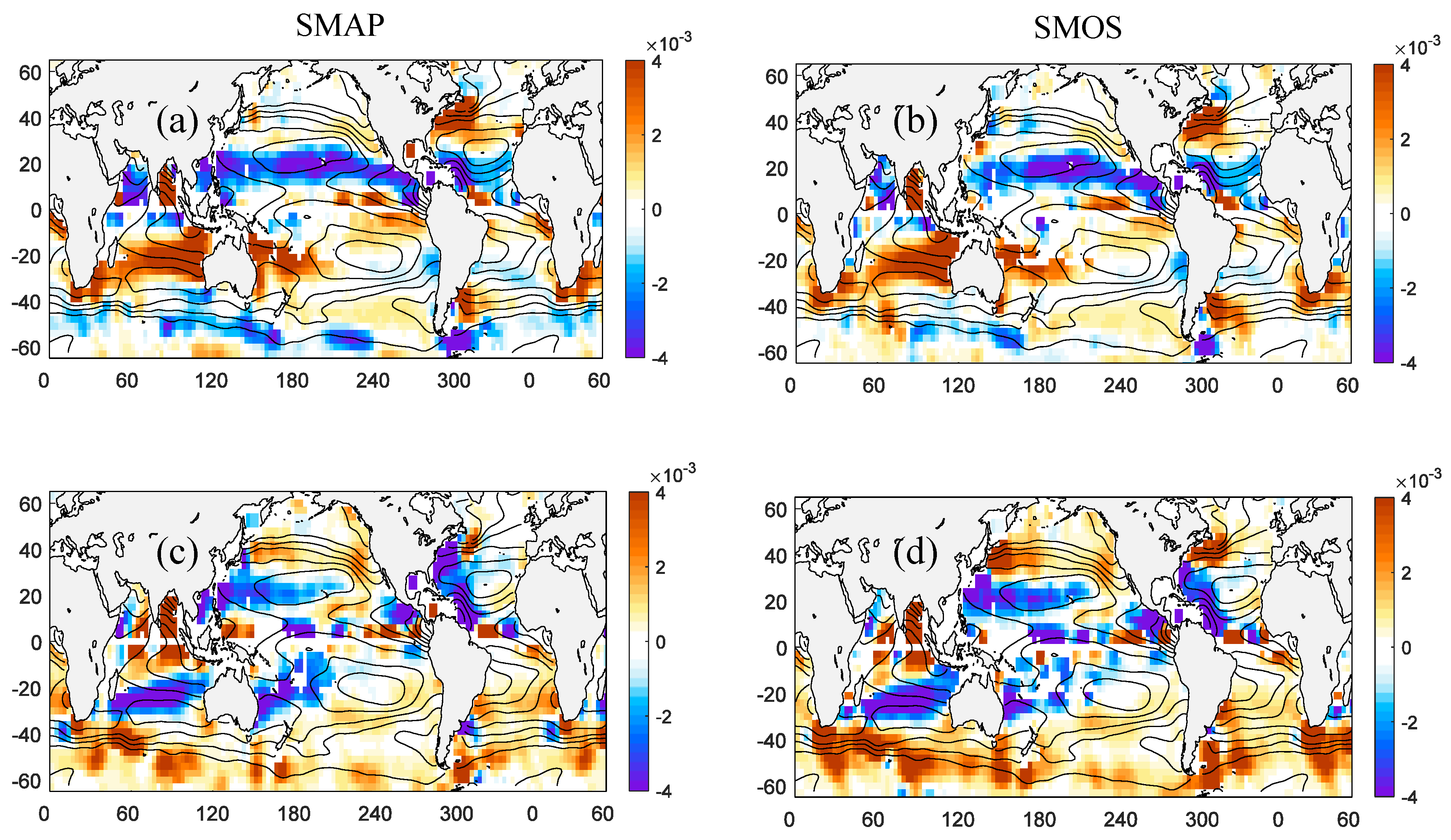
Estimates of the eddy salt flux through the eddy composite analysis are presented in Figure 4. Shown are meridional and zonal components of the eddy salt flux in the surface mixed layer estimated from both SMAP and SMOS SSS datasets.
The first thing to note in Figure 4 is that the estimates of the eddy salt flux agree very well between the two satellites and show physically meaningful structure. This includes both the meridional and zonal components of the flux. In each of the five subtropical gyres (identified by the subtropical SSS maxima), the eddy flux is divergent—eddies pump salt out of the gyre. The meridional salt transport is equatorward on the equatorward side of the gyre and poleward on the poleward side. The zonal component also contributes to this process, although its spatial structure is more complicated. In the NP, South Pacific (SP), and NA, the zonal component is generally eastward (positive) over the eastern side of the gyre and westward (negative) over the westward side. In the South Atlantic (SA), the zonal component is eastward (positive) over the eastern side of the gyre. In the SIO, the zonal component is westward (negative) over the equatorward limb of the subtropical gyre, which is consistent with the direction of the mean SSS gradient (the mean isohalines are tilted on the horizontal plane; the mean SSS is increasing toward the west). Overall, we can see that the zonal component of the flux appears significant in the regions of strong zonal background SSS gradients, which is generally consistent with the “gradient-flux” relationship [15]. In addition, in the subtropical gyres, the meridional structure of the meridional component of the eddy salt flux is strongly asymmetric in magnitude. The flux is one order of magnitude larger over the equatorward side of the gyre than over the poleward side. The exception is probably the South Pacific (SP), where the meridional flux is quite weak on both sides of the subtropical gyre. In the tropics, eddies tend to pump salt into the areas of low SSS, such as in the eastern Pacific Fresh Pool [11]. There, the meridional salt transport is equatorward (negative) on the poleward side of the pool and poleward (positive) on the equatorward side (Figure 4a); thus, the transport is convergent. The same feature can be observed in the tropical SIO. The meridional transport is equatorward (positive) on the poleward side of the Indian Ocean fresh pool, along about 20°S, and poleward (negative) on the equatorward side, just south of the Equator. Eddy fluxes in the sub-polar gyres are substantially smaller than in the tropics and subtropics. In the Southern Ocean, the eddy salt transport is poleward across the Antarctic Circumpolar Current (ACC) with the largest cross-ACC transport occurring in the Indian Ocean sector (Figure 4a). The large poleward flux across the ACC suggests that eddies act to weaken strong background salinity gradients associated with the Sub-Antarctic Front (SAF).
Discrepancies in the eddy salt flux estimates from the two satellite missions start to accumulate at higher latitudes. One such area where the discrepancies are quite significant is in the Southern Ocean, particularly along the ACC where the meridional (zonal) eddy fluxes estimated from SMOS data are generally smaller (larger) than those estimated from SMAP data. Some quantitative differences are also observed in and around the Brazil–Malvinas Confluence Zone in the SA and in the sub-polar NP and NA. These discrepancies between the two datasets can be due to insufficient spatial resolution. Eddy length scales generally decrease poleward with latitude and at high latitudes may not be well resolved in the present datasets. Alternatively, the discrepancies can be related to large errors in SSS retrievals. Due to the poor sensitivity of satellite radiometer to SSS in cold water, the level of noise in satellite retrievals at high latitudes increases dramatically. Then, the amount of averaging performed to construct eddy composites may not be adequate to suppress the noise. It is important to emphasize that the discrepancies in the eddy flux estimates are solely due to discrepancies in the satellite SSS datasets, as all other data (SLA maps, mesoscale eddy dataset) and procedures are exactly the same.
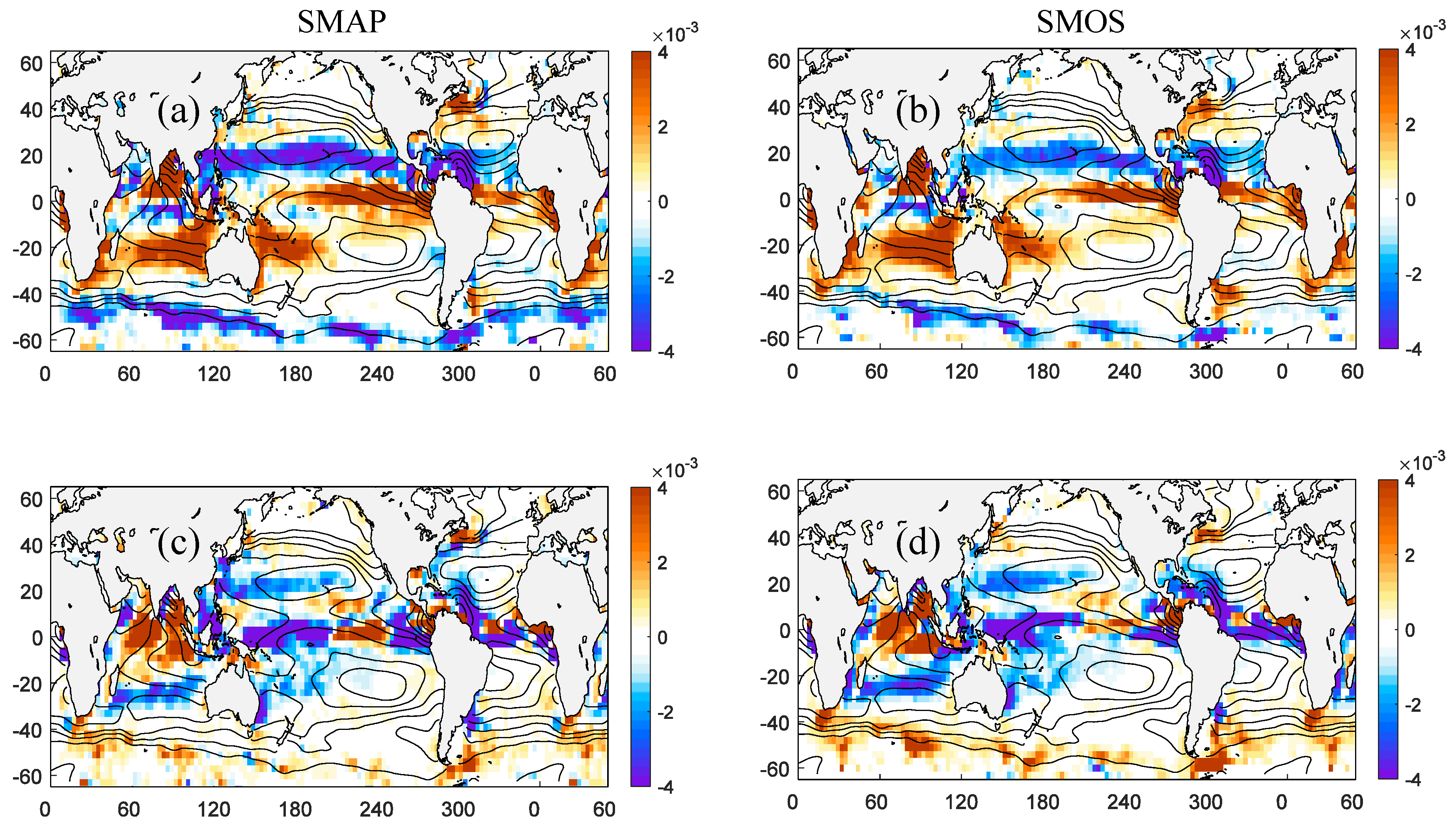
3.3. Eddy Salt Transport by Mean of Eddy Covariance
Next, we estimate the eddy salt flux as a covariance of salinity and velocity fluctuations at a point as defined by Equation (2). To increase the statistical significance of our estimates and for comparison with previous analysis, the covariances (2) are averaged in 3°-longitude × 3°-latidude bins. In addition, we use the full range of SMOS data spanning the period from 2011 to 2019. The results are displayed in Figure 5.
The maps of the eddy salt fluxes from SMAP and SMOS nearly mirror each other. Again, some quantitative differences are observed in the Southern Ocean along the ACC, where SMOS data demonstrate systematically lower meridional fluxes and somewhat stronger zonal fluxes. This can partly be related to the longer period of averaging in the case of SMOS data and/or higher level of noise. Other than that, the comparison is remarkably good. In addition, we can observe quite large meridional and zonal salt fluxes in the near-equatorial region, particularly in the Pacific Ocean, which are likely related to the signal of Tropical Instability Waves (TIWs) [16], not captured by the eddy composite analysis (Figure 4). We also note that the zonal salt transport is divergent in the central equatorial Pacific (eddies mix salt out of the central Pacific and into both the western and eastern Pacific freshwater pools) and convergent further east (change of sign at around 120°W). The results in the near equatorial region have to be interpreted with caution though. The geostrophic balance breaks at the Equator (the Coriolis force vanishes) and the altimetry-derived estimates of the zonal geostrophic flow near the Equator, where the Coriolis force is weak, can be less accurate [35].
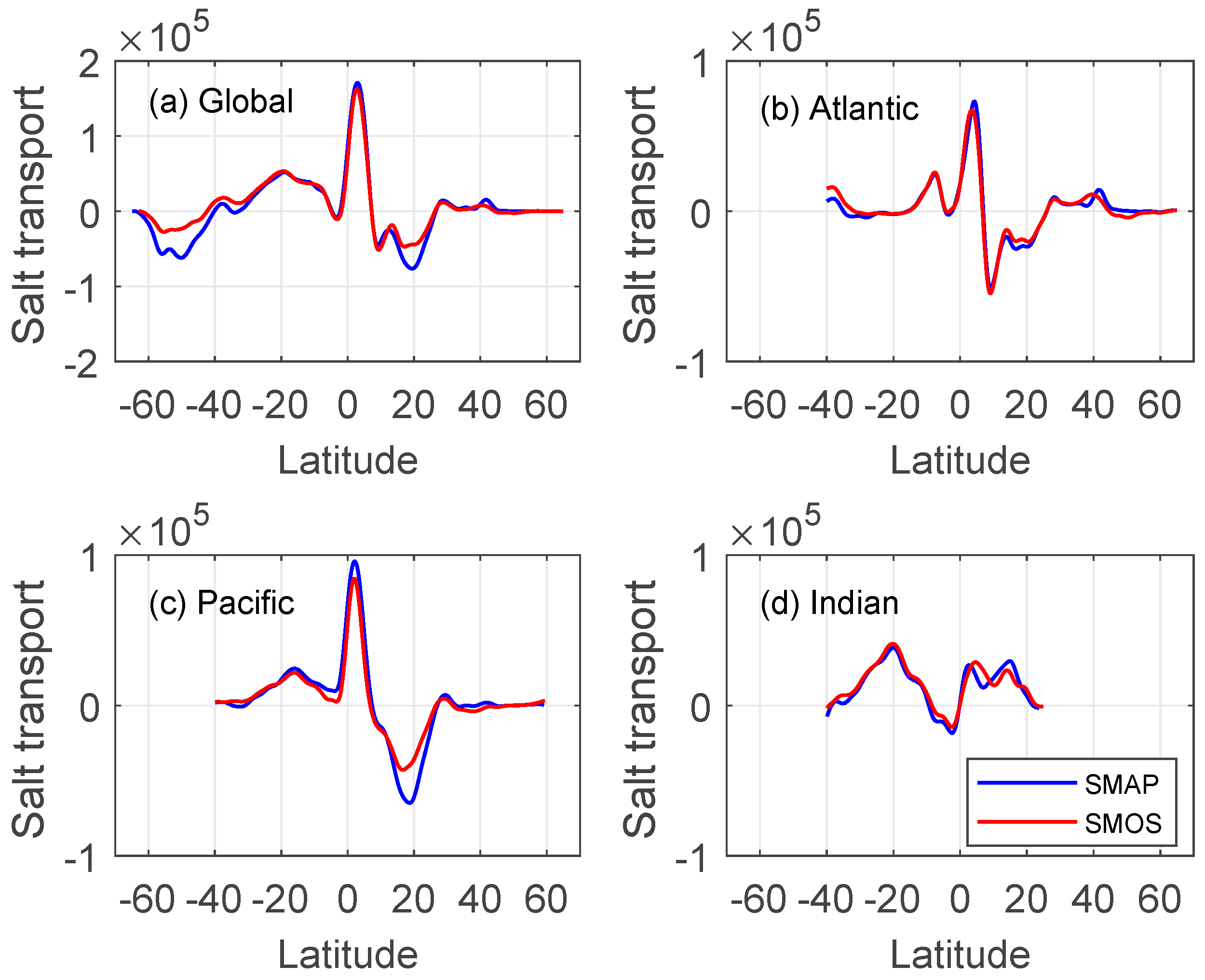
For a more quantitative comparison, Figure 6 shows the zonally integrated meridional transport of salt in the three oceans and globally as a function of latitude. Here, we use estimates from the covariance analysis (Figure 5). The agreement between the two satellites is striking, particularly in the Atlantic and Indian Oceans. Quantitative discrepancies are in the subtropical Pacific (Figure 6c) and in the Southern Ocean between 60 and 40°S (Figure 6a), where the eddy transport is weaker by about 30% in SMOS estimates. Comparing the eddy salt transport in different basins, we also note large maxima in the Atlantic and Pacific near-equatorial belt peaking at about 2–3°N. These are the largest peaks and are likely associated with the signal of TIWs that are active in both the Atlantic and Pacific [21,36]. Similar peaks have been observed in the Pacific Ocean (but not in the Atlantic) in a modeling study by [37], who also attributed the peaks to the signal of TIWs. It appears that TIWs can play a very significant role in the local salt budget in the tropical Pacific and Atlantic.
3.4. Implications for the Subtropical SSS Maxima
To put our estimates into perspective, we consider the role of mesoscale eddies in balancing the mean E–P flux in the interiors of the subtropical gyres. The importance of the eddy salt transport to the mean salinity distribution in the subtropical gyres has been investigated in a number of studies [7,10,25,33,38], all using different data and techniques. The results vary significantly. Evaporation (E) typically exceeds precipitation (P) within the subtropical gyres where local SSS maxima exist [39]. To maintain a steady-state distribution of SSS, the E–P flux, which acts to increase surface salinity, should be compensated by oceanic processes, which would transfer the excess of salt out of the SSS-maximum regions [10]. Among these oceanic processes is the eddy transport of salt. Following the approach by [10], we assess the relative role mesoscale eddies play in the surface mixed layer in compensating the E–P flux.
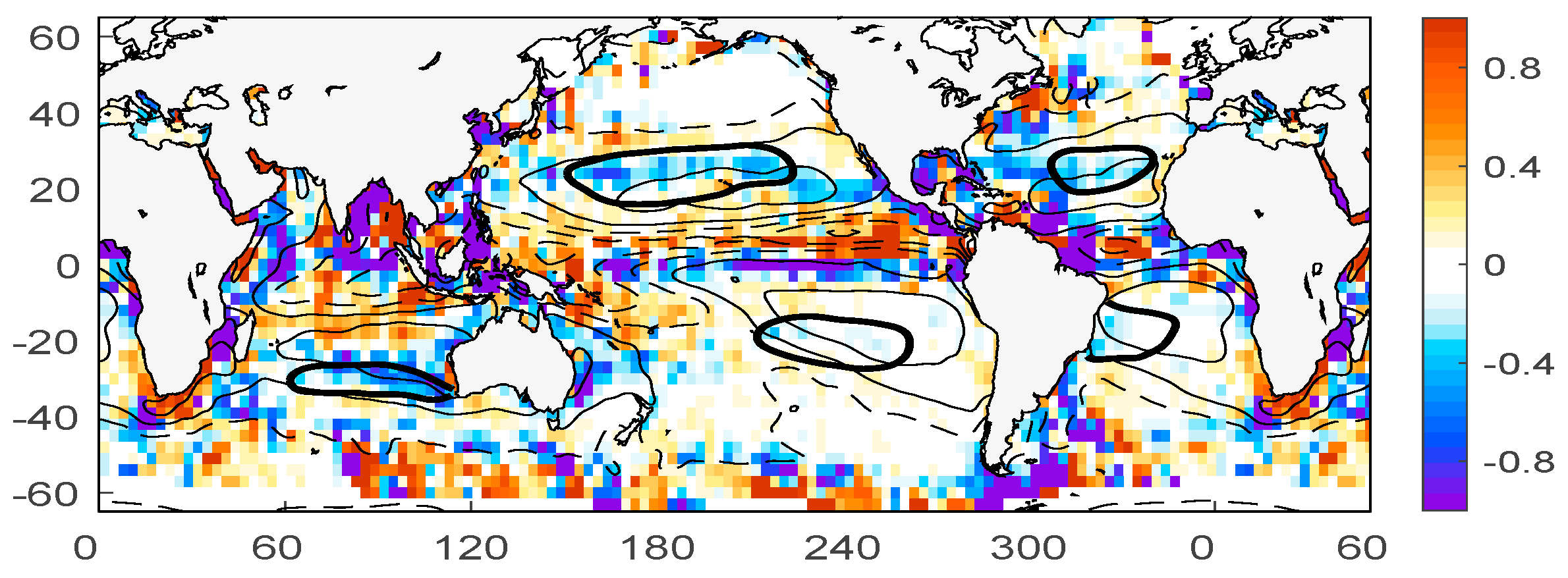
Figure 7 shows the divergence of salt due to eddy transport. Shown on top are contours of the mean E–P. The distribution of the divergence of the salt flux is patchy (taking a derivative in space amplifies small scales), but the large-scale patterns are apparent. The divergence of salt is negative in the five subtropical oceans, roughly coinciding with the SSS-maximum regions. These regions are defined in Figure 7 as the regions bounded by specific isohalines (black bold contours). They are 37 psu in the NA, 35 psu in the NP, 36.8 psu in the SA, 36.0 in the SP, and 35.6 in the SIO. The choice is somewhat subjective, yet it generally corresponds to the previous studies [39] and is suitable for further evaluation of the eddy effects. In each of the five SSS-maximum regions, we evaluate the contribution of the eddy salt flux and compare it to the surface forcing. The relevant terms in the surface mixed layer salinity budget are the eddy-induced divergence of salt, and the surface forcing, which is determined as the “virtual salt flux” [40], where is the reference salinity and is the mixed layer depth (MLD). The eddy salt flux divergence in each area is estimated as the integral over the area (equivalent to the flux through the boundary of the area) and is compared to the area integral of the surface forcing. The influence of the MLD variability is not taken into account, fixing it to the mean value of 50 m.
The percentage of the mean E–P flux balanced by the eddy salt flux in each of the five subtropical gyres is shown in Table 1. The highest surface forcing compensation is observed in the SIO and NP: around 21% and 15%, respectively. The NA also has a high percentage of the surface-forcing compensation of around 14%. The smallest values are in the SP and SA, where the eddy flux compensates for no more than 6% of the surface forcing. Likewise, we can see a very good agreement between SMAP and SMOS estimates.
Comparing our results to previous studies, we find generally similar results. The most relevant is probably the study by [7], who conducted a series of numerical experiments to evaluate the contributions of the eddy transport of salt to maintaining a quasi-steady-state balance in the subtropical SSS maxima. Their estimates of the surface forcing compensation also show significant regional differences, ranging from 10% in the SP to 25% in the SIO, which is comparable to our results. Using SMOS SSS data from 2010 to 2016, [20] obtained slightly higher surface forcing compensation rates, ranging from nearly 50% in the SIO to 12% in the SA. However, the quantitative comparison between different studies is complicated by several issues. One of these is that the bounded areas vary significantly from study to study, which affects both the integral of the eddy term and the surface forcing term [7]. Likewise, the results would depend on how mesoscale eddies are defined. Contrary to our study, [25] defined the eddy field as everything that is time varying, including the seasonal cycle. Although relatively small, the seasonal cycle and inter-annual variability can contribute to the estimates of the eddy term [37], perhaps explaining the larger numbers in [25]. However, overall, the regional characteristics and the differences seem to compare well to our results. Relatively low numbers in Table 1 also indicate that the eddy transport is not the only mechanism responsible for the compensation of the SSS increase due to excessive evaporation in the subtropics. Other oceanic processes are important, among which are the wind-driven Ekman transport as well as subsurface processes such as entrainment and mixing across the base of the mixed layer (e.g., [40,41,42]).
4. Discussion and Conclusions
In this study, we have diagnosed the eddy transport of salt in the surface mixed layer of the ocean from satellite observations of SLA and SSS. Given relatively large errors in satellite SSS retrievals, we used two products from two different satellite missions, SMAP and SMOS. We have also evaluated the eddy transport of salt using two methods. The first method is based on the so-called eddy composite analysis. As a result of the averaging over a large number of eddies in a given geographic area, composite eddies result in quite small standard errors (<0.02 psu in most cases), producing robust estimates of the associated transport of salt. The second method estimates the eddy transport of salt in a traditional way by computing pointwise covariances between eddy-induced velocity and SSS fluctuations.
Comparing between the two satellite missions, SMAP and SMOS, we find that the estimates of the eddy salt transport agree very well, particularly in the tropics and subtropics. The transport is divergent in the subtropical gyres (eddies pump salt out of the gyres) and convergent in the tropics. The estimates from the two satellites start to disagree regionally at higher latitudes, particularly in the Southern Ocean along the ACC, where estimates from SMOS data show systematically lower meridional fluxes but stronger zonal fluxes (Figure 5). Some quantitative differences are also observed in the western tropical Pacific (along ≈ 20°N) where SMOS data demonstrate somewhat weaker meridional transport. These discrepancies in the eddy salt transport estimates are exclusively due to discrepancies in the satellite SSS datasets, as all other data and procedures have been used the same. The discrepancies at high latitudes are likely related to a considerable increase in the level of noise in the satellite retrievals (because of poor sensitivity of the satellite radiometer to SSS in cold water), which may affect the computed correlations or can be due to resolution issues. Eddy length scales generally decrease with increasing latitude (Figure 3d) and at high latitudes may not be well resolved in the present SSS datasets. Yet, given relatively small quantitative differences between the estimates from the two satellite missions, it is quite difficult to say which one is more accurate in depicting mesoscale SSS variability. In addition, there is no compelling theory that could be used to assess the expectations, nor are there adequate high-resolution observational programs for a direct comparison, particularly at high latitudes where the largest differences are observed. The accuracy can be (and likely is) regionally dependent, e.g., one satellite can provide more accurate data in one area and less accurate in the other, and for various reasons (for example, SMOS observations seem to be much more affected by radio frequency interference (RFI) and land contamination, which can be a source of large errors in SSS retrievals as far as 1000 km from the coast [16,20]). Overall, we find the comparison very satisfactory, without discrediting either satellite.
The comparison between the two methods (Figure 4 and Figure 5) seems to validate the assumption that the ocean is densely packed with mesoscale eddies, and the eddy transport is mainly due to large eddies. The latter is to be expected. Both theoretical arguments [43,44] and observational and modeling studies suggest that horizontal eddy fluxes in the ocean are dominated by large mesoscale eddies. In particular, [45] explored spectral characteristics of the eddy heat fluxes in the Pacific Ocean from satellite sea surface temperature (SST) and SLA data and found that the fluxes were dominated by contributions from length scales that were very close to the length scales of large mesoscale eddies identified in the eddy dataset by [9]. Likewise, numerical experiments by [46] have demonstrated that horizontal eddy fluxes arise mainly due to large mesoscale eddies and change only slightly when the model resolution is increased. These arguments make the analysis of the eddy salt fluxes from satellite observations very relevant.
The comparison between the two methods (Figure 4 and Figure 5) also emphasizes the physical mechanism responsible for the eddy transport of salt—that is, horizontal advection of background SSS gradient by eddy velocities. This results in the eddy-induced velocity and SSS perturbations being generally in phase over the eddy wavelength (Figure 3), providing necessary conditions for non-zero correlation [32]. One possible implication of our analysis is also a potential to reconstruct a three-dimensional (3D) structure of the eddy-induced transport of salt using in situ data, such as Argo profiling float data. Although the spatial resolution of the Argo data is obviously not sufficient for direct estimates (such as Equation (2)), it might be quite sufficient to construct 3D eddy composites (e.g., [33]), which in turn can be used to reconstruct a 3D distribution of the eddy transport (similar to a one-layer reconstruction such as in Section 3.2). Such a reconstruction would be meaningful, as shown here by the comparison with direct estimates at the sea surface. This technique, yet for the eddy heat flux, was used by [47] to reconstruct the eddy transport of heat across a zonal section (47°N) in the NA.
Our analysis also confirms that the eddy transport of salt (or, equivalently, freshwater) is an essential component of the marine hydrological cycle. The regions of major eddy transport of salt identified in our study occur in the tropical belt, across the equatorward limbs of the subtropical gyres, and across the ACC. The eddy salt transport is poleward across the ACC with the largest transport taking place in the Indian Ocean sector. The large poleward transport across the ACC suggests that eddies act to weaken strong background salinity gradients associated with the Sub-Antarctic Front. The eddy transport in the sub-polar gyres is substantially smaller than the eddy transport in the tropics and subtropics. We also note that the zonal component of the eddy salt transport is quite significant, particularly over the western and eastern boundaries of the gyres and in the near-equatorial belt, where strong zonal gradients of SSS are observed.
To put our estimates into perspective, we quantified the relative role of the eddy transport in balancing the climatological mean E–P flux in the subtropical gyres, where local SSS maxima exist. The eddy transport of salt plays an essential role in balancing the E–P flux in each of the five gyres, yet with significant regional differences. The highest surface forcing compensation, around 21%, is observed in the SIO. The lowest surface forcing compensation, around 5%, is observed in the SP and SA. The numbers compare favorably to previous studies [7,25], based on different data and techniques, adding confidence to our results.
Our study demonstrates that the possibility to characterize and quantify the eddy transport of salt in the ocean surface layer can rely on the use of satellite observations of SSS. Here, we estimated the time mean effects of eddies based on less than ten years of satellite data. However, recent studies suggest that temporal variability in the eddy salt transport is particularly important and can be related to climate changes [3]. This interaction between the scales is not yet well known and understood. Therefore, a continuation of satellite observations of SSS with mesoscale resolution to assemble at least several decades of data is needed to help understand these processes and scale interactions.
While past (Aquarius) and current (SMAP and SMOS) satellite missions have helped to better understand how the ocean salinity operates, a considerable part of the SSS variability associated with mesoscale and sub-mesoscale processes remains missing. Current satellite missions still have limited spatial resolution and limited accuracy for mesoscale monitoring, particularly at high latitudes. Thus, new technologies and observation approaches are required to improve resolution capabilities of future satellite missions in order to observe mesoscale variability, improve the signal-to-noise ratio, and extend these capabilities to the polar oceans [17].
Author Contributions
Conceptualization, O.M.; methodology, O.M.; validation and data analysis, O.M., P.H. and V.M.; writing—original draft preparation, O.M.; writing—review and editing, O.M., P.H. and V.M.; funding acquisition, O.M. All authors have read and agreed to the published version of the manuscript.
Funding
This research was supported by the National Aeronautics and Space Administration (NASA) Physical Oceanography Program through grant NNX17AK06G and grant NNX17AH26G.
Institutional Review Board Statement
Not applicable.
Informed Consent Statement
Not applicable.
Data Availability Statement
Data used in this study are available as follows. SMAP salinity data are produced by Remote Sensing Systems and sponsored by the NASA Ocean Salinity Science Team. Data are available at www.remss.com. The L3_DEBIAS_LOCEAN_v4 Sea Surface Salinity maps have been produced by LOCEAN/IPSL (UMR CNRS/UPMC/IRD/MNHN) laboratory and ACRI-st company that participate in the Ocean Salinity Expertise Center (CECOS) of Centre Aval de Traitement des Donnees SMOS (CATDS). The data are available at https://0-doi-org.brum.beds.ac.uk/10.17882/52804#69293. Sea level anomaly (SLA) observations from satellite altimetry and the respective geostrophic velocity fields are provided by the Copernicus Marine Environment Monitoring Service (CMEMS) at http://marine.copernicus.eu. Mesoscale Eddy Trajectory Atlas products were produced by SSALTO/DUACS and distributed by AVISO+ (https://www.aviso.altimetry.fr/) with support from CNES, in collaboration with Oregon State University with support from NASA. Precipitation data were obtained from the Global Precipitation Climatology Project (GPCP) at https://rda.ucar.edu/datasets/ds728.3/. Evaporation data were obtained from the Objectively Analyzed air-sea Fluxes project (OAFlux) at http://oaflux.whoi.edu.
Acknowledgments
We thank three anonymous reviewers for their thoughtful comments. IPRC/SOEST contribution 1502/11232.
Conflicts of Interest
The authors declare no conflict of interest.
References
- U.S. CLIVAR Office. Report of the U.S. CLIVAR Salinity Science Working Group; U.S. CLIVAR Report; U.S. CLIVAR Office: Washington, DC, USA, 2007; p. 46. [Google Scholar]
- Schmitt, R.W. Salinity and the Global Water Cycle. Oceanography 2008, 21, 12–19. [Google Scholar] [CrossRef]
- Durack, P.J. Ocean Salinity and the Global Water Cycle. Oceanography 2015, 28, 20–31. [Google Scholar] [CrossRef] [Green Version]
- Yang, Q.; Dixon, T.; Myers, P.; Bonin, J.; Chambers, D.; Broeke, M.R.; Ribergaard, M.H.; Mortensen, J. Recent increases in Arctic freshwater flux affects Labrador Sea convection and Atlantic overturning circulation. Nat. Commun. 2016, 7. [Google Scholar] [CrossRef] [PubMed] [Green Version]
- Lukas, R.; Lindstrom, E. The mixed layer of the western equatorial Pacific Ocean. J. Geophys. Res. 1991, 96, 3343–3357. [Google Scholar] [CrossRef]
- Vinogradova, N.T.; Ponte, R.M. Clarifying the link between surface salinity and freshwater fluxes on monthly to interannual time scales. J. Geophys. Res. Oceans 2013, 118, 3190–3201. [Google Scholar] [CrossRef]
- Busecke, J.J.M.; Abernathey, R.P.; Gordon, A.L. Lateral Eddy Mixing in the Subtropical Salinity Maxima of the Global Ocean. J. Phys. Oceanogr. 2017, 47, 737–754. [Google Scholar] [CrossRef]
- Ferrari, R.; Wunsch, C. Ocean circulation kinetic energy: Reservoirs, sources, and sinks. Annu. Rev. Fluid Mech. 2009, 41, 253–282. [Google Scholar] [CrossRef] [Green Version]
- Chelton, D.B.; Schlax, M.G.; Samelson, R.M. Global Observations of Nonlinear Mesoscale Eddies. Prog. Oceanogr. 2011, 91, 167–216. [Google Scholar] [CrossRef]
- Gordon, A.L.; Giulivi, C.F. Ocean eddy freshwater flux convergence into the North Atlantic Subtropics. J. Geophys. Res. Oceans 2014, 119, 3327–3335. [Google Scholar] [CrossRef]
- Delcroix, T.; Chaigneau, A.; Soviadan, D.; Boutin, J.; Pegliasco, C. Eddy-induced salinity changes in the tropical Pacific. J. Geophys. Res. Oceans 2019, 124, 374–389. [Google Scholar] [CrossRef]
- Busecke, J.; Gordon, A.L.; Li, Z.; Bingham, F.M.; Font, J. Subtropical surface layer salinity budget and the role of mesoscale turbulence. J. Geophys. Res. Oceans 2014, 119, 4124–4140. [Google Scholar] [CrossRef] [Green Version]
- Treguier, A.M.; Deshayes, J.; Lique, C.; Dussin, R.; Molines, J.M. Eddy contributions to the meridional transport of salt in the North Atlantic. J. Geophys. Res. Oceans 2012, 117. [Google Scholar] [CrossRef] [Green Version]
- Jayne, S.R.; Marotzke, J. The oceanic eddy heat transport. J. Phys. Oceanogr. 2002, 32, 3328–3345. [Google Scholar] [CrossRef]
- Bachman, S.; Fox-Kemper, B. Eddy parameterization challenge suite I: Eddy spindown. Ocean Model. 2013, 64, 12–28. [Google Scholar] [CrossRef]
- Reul, N.; Grodsky, S.A.; Arias, M.; Boutin, J.; Catany, R.; Chapron, B.; Amico, F.; Dinnat, E.; Donlon, C.; Fore, A.; et al. Sea surface salinity estimates from spaceborne L-band radiometers: An overview of the first decade of observation (2010–2019). Remote Sens. Environ. 2020, 242. [Google Scholar] [CrossRef]
- Vinogradova, N.; Lee, T.; Boutin, J.; Drushka, K.; Fournier, S.; Sabia, R.; Stammer, D.; Bayler, E.; Reul, N.; Gordon, A.; et al. Satellite Salinity Observing System: Recent Discoveries and the Way Forward. Front. Mar. Sci. 2019, 6. [Google Scholar] [CrossRef]
- Meissner, T.; Wentz, F.; Vine, D.; Lagerloef, G.; Lee, T. Estimate of uncertainties in the Aquarius salinity retrievals. In Proceedings of the Geoscience and Remote Sensing Symposium (IGARSS), Milan, Italy, 26–31 July 2015; pp. 5324–5327. [Google Scholar] [CrossRef]
- Kao, H.Y.; Lagerloef, G.S.E.; Lee, T.; Melnichenko, O.; Meissner, T.; Hacker, P. Assessment of Aquarius Sea Surface Salinity. Remote Sens. 2018, 10, 1341. [Google Scholar] [CrossRef] [Green Version]
- Boutin, J.; Vergely, J.L.; Thouvenin, M.C.; Supply, A.; Khvorostyanov, D. SMOS SSS L3 maps generated by CATDS CEC LOCEAN debias V4.0. SEANOE 2019. [Google Scholar] [CrossRef]
- Lee, T.; Lagerloef, G.; Gierach, M.M.; Kao, H.Y.; Yueh, S.; Dohan, K. Aquarius reveals salinity structure of tropical instability waves. Geophys. Res. Lett. 2019, 39, L12610. [Google Scholar] [CrossRef]
- Maes, C.; Dewitte, B.; Sudre, J.; Garcon, V.; Varillon, D. Small-scale features of temperature and salinity surface fields in the Coral Sea. J. Geophys. Res. Oceans 2013, 118, 5426–5438. [Google Scholar] [CrossRef] [Green Version]
- Kolodziejczyk, N.; Hernandez, O.; Boutin, J.; Reverdin, G. SMOS salinity in the subtropical North Atlantic salinity maximum: 2. Two-dimensional horizontal thermohaline variability. J. Geophys. Res. Oceans 2015, 120, 972–987. [Google Scholar] [CrossRef] [Green Version]
- Melnichenko, O.; Amores, A.; Maximenko, N.; Hacker, P.; Potemra, J. Signature of mesoscale eddies in satellite sea surface salinity data. J. Geophys. Res. Oceans 2017, 122, 1416–1424. [Google Scholar] [CrossRef]
- Qu, T.; Lian, Z.; Nie, X.; Wei, Z. Eddy-induced meridional salt flux and its impacts on the sea surface salinity maxima in the southern subtropical oceans. Geophys. Res. Lett. 2019, 46, 11292–11300. [Google Scholar] [CrossRef]
- Meissner, T.; Wentz, F.J.; Manaster, A.; Lindsley, R. Remote Sensing Systems SMAP Ocean Surface Salinities [Level 2C, Level 3 Running 8-day, Level 3 Monthly], Version 4.0 Validated Release; Remote Sensing Systems: Santa Rosa, CA, USA, 2019. [Google Scholar] [CrossRef]
- Aviso+Altimetry. Mesoscale Eddy Trajectory Atlas Product Handbook; Aviso+Altimetry: Ramonville St Agne, France, 2019. [Google Scholar]
- Schlax, M.G.; Chelton, D.B. The “Growing Method” of Eddy Identification and Tracking in Two and Three Dimensions; Ocean and Atmospheric Sciences, College of Earth, Oregon State University: Corvallis, OR, USA, 2016. [Google Scholar]
- Huffman, G.J.; Bolvin, D.T.; Adler, R.F. GPCP version 1.2 One-Degree Daily Precipitation Data Set. In Research Data Archive at the National Center for Atmospheric Research; Computational and Information Systems Laboratory: Boulder, CO, USA, 2016. [Google Scholar] [CrossRef]
- Yu, L.; Weller, R.A. Objectively Analyzed air-sea heat Fluxes for the global ice-free oceans (1981-2005). Bull. Am. Meteorol. Soc. 2007, 88, 527–529. [Google Scholar] [CrossRef] [Green Version]
- Hausmann, U.; Czaja, A. The observed signature of mesoscale eddies in sea surface temperature and the associated heat transport. Deep-Sea Res. I 2012, 70, 60–72. [Google Scholar] [CrossRef]
- Roemmich, D.; Gilson, J. Eddy transport of heat and thermocline waters in the North Pacific: A key to interannual/decadal climate variability? J. Phys. Oceanogr. 2001, 31, 675–687. [Google Scholar] [CrossRef]
- Amores, A.; Melnichenko, O.; Maximenko, N. Coherent mesoscale eddies in the North Atlantic subtropical gyre: 3D structure and transport with application to the salinity maximum. J. Geophys. Res. 2017, 122, 23–41. [Google Scholar] [CrossRef]
- Thompson, A.F.; Young, Y.R. Scaling Baroclinic Eddy Fluxes: Vortices and Energy Balance. J. Phys. Oceanogr. 2006, 36, 720–738. [Google Scholar] [CrossRef]
- Sudre, J.; Maes, C.; Garçon, V. On the global estimates of geostrophic and Ekman surface currents. Limnol. Oceanogr. Fluids Environ. 2013, 3. [Google Scholar] [CrossRef] [Green Version]
- Lee, T.; Lagerloef, G.; Kao, H.Y.; Phaden, M.J.; Willis, J.; Gierach, M.M. The influence of salinity on tropical Atlantic instability waves. J. Geophys. Res. Oceans 2014, 119, 8375–8394. [Google Scholar] [CrossRef]
- Treguier, A.M.; Deshayes, J.; Sommer, J.; Lique, C.; Madec, G.; Penduff, T.; Molines, J.M.; Barnier, B.; Bourdalle, B.R.; Talandier, C. Meridional transport of salt in the global ocean from an eddy resolving model. Ocean Sci. 2014, 10, 243–255. [Google Scholar] [CrossRef] [Green Version]
- Bryan, F.; Bachman, S. Isohaline Salinity Budget of the North Atlantic Salinity Maximum. J. Phys. Oceanogr. 2015, 45, 724–736. [Google Scholar] [CrossRef]
- Gordon, A.L.; Giulivi, A.L.; Busecke, J.; Bingham, F.M. Differences among subtropical surface salinity patterns. Oceanography 2015, 28, 32–39. [Google Scholar] [CrossRef] [Green Version]
- Farrar, J.T.; Rainvill, L.; Plueddemann, A.J.; Kessler, W.S.; Lee, C.; Hodges, B.A.; Schmitt, R.W.; Edson, J.B.; Riser, S.C.; Erikse, C.C.; et al. Salinity and temperature balances at the SPURS Central mooring during fall and winter. Oceanography 2015, 28, 56–65. [Google Scholar] [CrossRef] [Green Version]
- Hasson, A.; Delcroix, T.; Boutin, J. Formation and variability of the South Pacific Sea Surface Salinity maximum in recent decades. J. Geophys. Res. Oceans 2013, 118, 5109–5116. [Google Scholar] [CrossRef] [Green Version]
- Katsura, S.; Oka, E.; Qiu, B.; Schneider, N. Formation and Subduction of North Pacific Tropical Water and Their Interannual Variability. J. Phys. Oceanogr. 2013, 43, 2400–2415. [Google Scholar] [CrossRef] [Green Version]
- Larichev, V.; Held, I.M. Eddy amplitudes and fluxes in a homogeneous model of fully developed baroclinic instability. J. Phys. Oceanogr. 1995, 25, 2285–2297. [Google Scholar] [CrossRef] [Green Version]
- Thompson, A.F.; Young, W.R. Two-layer baroclinic eddy heat fluxes: Zonal flows and energy balance. J. Atmos. Sci. 2007, 64, 3214–3231. [Google Scholar] [CrossRef] [Green Version]
- Aberhatney, R.; Wortham, C. Phase speed cross spectra of eddy heat fluxes in the eastern Pacific. J. Phys. Oceanogr. 2015, 45, 1285–1301. [Google Scholar] [CrossRef] [Green Version]
- Capet, X.; Williams, J.C.; Molemaker, M.J.; Shchepetkin, A.F. Mesoscale to submesoscale transition in the California Current System. Part 1: Flow structure and eddy flux. J. Phys. Oceanogr. 2008, 38, 29–43. [Google Scholar] [CrossRef] [Green Version]
- Müller, V.; Melnichenko, O. Decadal changes of meridional eddy heat transport in the subpolar North Atlantic derived from satellite and in situ observations. J. Geophys. Res. Oceans 2020, 125. [Google Scholar] [CrossRef]
Figure 1.
(a) Soil Moisture Active-Passive (SMAP) sea surface salinity (SSS) (psu) and (b) Soil Moisture and Ocean Salinity (SMOS) SSS (psu) fields for the week centered on April 30, 2016. The inserts (c,d) show local zooms of (a,b), respectively, in the region (25–15°S, 90–100°E) in the South Indian Ocean (black rectangle).

Figure 2.
(Top) SSS anomalies (psu) associated with anticyclonic (a,c) and cyclonic (b,d) composite eddy in the South Indian Ocean (25–15°S, 90–100°E). The left and right pairs of panels compare SMAP (left) and SMOS (right) SSS analyses. (Bottom, e–h) Zonal sections across the composite eddies. In each panel, the green and blue curves show the eddy meridional velocity (cm/s) and SSS anomaly (psu), respectively. The blue (green) shaded area represents standard errors of the composite SSS (meridional velocity).

Figure 3.
(a) Schematic illustration showing how eddy fluxes of salt are computed globally from eddy composites reconstructed in 6°-longitude × 6°-latitude bins. Blue lines show the boundaries of the bins. The insert illustrates how the meridional flux of salt in each bin is estimated. The flux through the zonal section of the bin is given by the flux per a composite eddy multiplied by the number of eddies that can fit into the section (blue and red circles show schematically cyclonic (C) and anticyclonic (A) eddies, respectively). (b) Number of eddy realizations observed in 6°-longitude × 6°-latitude bins over the 4-year period from April 2015 to May 2019. (c) Eddy root-mean-square (RMS) velocity (cm/s), estimated as 0.71 of the mean speed-based amplitude. (d) Mean eddy speed-based radius scale (km).

Figure 4.
Eddy salt fluxes in the surface mixed layer estimated through the eddy composite analysis from SMAP (a,c) and SMOS (b,d) SSS data during the common observational period from 2015 to 2019. (a,b) Meridional salt flux. Positive (negative) values indicate northward (southward) salt flux. (c,d) Zonal salt flux. Positive (negative) values indicate eastward (westward) salt flux. Units are kg m−2 s−1. Shown on top of each figure are contours of mean SSS (C.I. = 0.5 psu).

Figure 5.
Eddy salt fluxes in the surface mixed layer estimated by covariance analysis from SMAP (a,c) and SMOS (b,d) SSS data. (a,b) Meridional salt flux. Positive (negative) values indicate northward (southward) salt flux. (c,d) Zonal salt flux. Positive (negative) values indicate eastward (westward) salt flux. Units are kg m−2 s−1. Shown on top of each figure are contours of mean SSS (C.I. = 0.5 psu).

Figure 6.
Zonally integrated eddy salt fluxes in the surface mixed layer evaluated (a) globally and over the (b) Atlantic, (c) Pacific, and (d) Indian Ocean from SMAP (blue) and SMOS (red) SSS data. The fluxes are in 1-m layer so the units are kg m−1 s−1.
Figure 6.
Zonally integrated eddy salt fluxes in the surface mixed layer evaluated (a) globally and over the (b) Atlantic, (c) Pacific, and (d) Indian Ocean from SMAP (blue) and SMOS (red) SSS data. The fluxes are in 1-m layer so the units are kg m−1 s−1.

Figure 7.
Divergence of the eddy salt flux, computed from SMOS SSS data. Units are 10−8 kg m−3 s−1. Negative values represent salt divergence. Shown on top are contours of mean evaporation (E)–precipitation (P). C.I. = 0.5 mm day−1, zero contour is omitted. Solid contours show E–P > 0 (evaporation exceed precipitation), dashed: E–P < 0 (precipitation exceed evaporation). The subtropical SSS-maximum areas are bounded by contours of mean SSS (bold contours): 37 psu in the North Atlantic, 35 psu in the North Pacific, 36.8 psu in the South Atlantic, 36.0 in the South Pacific, and 35.6 in the South Indian Ocean.


Table 1.
Percentage of the E–P flux in the subtropical SSS-maxima balanced by the eddy salt transport.
Table 1.
Percentage of the E–P flux in the subtropical SSS-maxima balanced by the eddy salt transport.
| SIO | NA | SA | NP | SP | |
|---|---|---|---|---|---|
| SMAP | 21 | 14 | 3 | 15 | 6 |
| SMOS | 20 | 11 | 5 | 12 | 4 |
Publisher’s Note: MDPI stays neutral with regard to jurisdictional claims in published maps and institutional affiliations. |
© 2021 by the authors. Licensee MDPI, Basel, Switzerland. This article is an open access article distributed under the terms and conditions of the Creative Commons Attribution (CC BY) license (http://creativecommons.org/licenses/by/4.0/).
Share and Cite
MDPI and ACS Style
Melnichenko, O.; Hacker, P.; Müller, V. Observations of Mesoscale Eddies in Satellite SSS and Inferred Eddy Salt Transport. Remote Sens. 2021, 13, 315. https://0-doi-org.brum.beds.ac.uk/10.3390/rs13020315
AMA Style
Melnichenko O, Hacker P, Müller V. Observations of Mesoscale Eddies in Satellite SSS and Inferred Eddy Salt Transport. Remote Sensing. 2021; 13(2):315. https://0-doi-org.brum.beds.ac.uk/10.3390/rs13020315
Chicago/Turabian StyleMelnichenko, Oleg, Peter Hacker, and Vasco Müller. 2021. "Observations of Mesoscale Eddies in Satellite SSS and Inferred Eddy Salt Transport" Remote Sensing 13, no. 2: 315. https://0-doi-org.brum.beds.ac.uk/10.3390/rs13020315
Note that from the first issue of 2016, this journal uses article numbers instead of page numbers. See further details here.