New Method for Automated Quantification of Vertical Spatio-Temporal Changes within Gully Cross-Sections Based on Very-High-Resolution Models


Abstract
:
1. Introduction
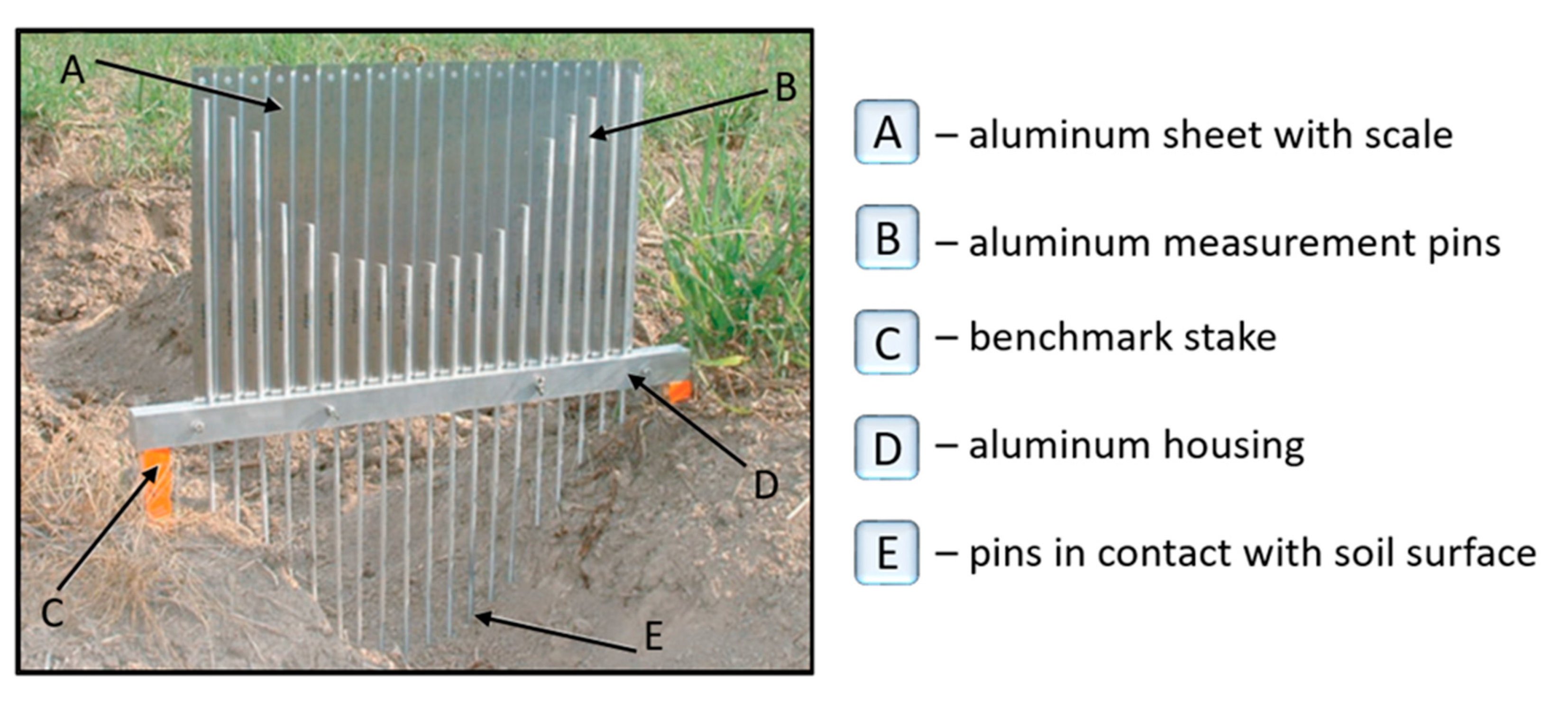
2. Study Area
3. Materials and Methods
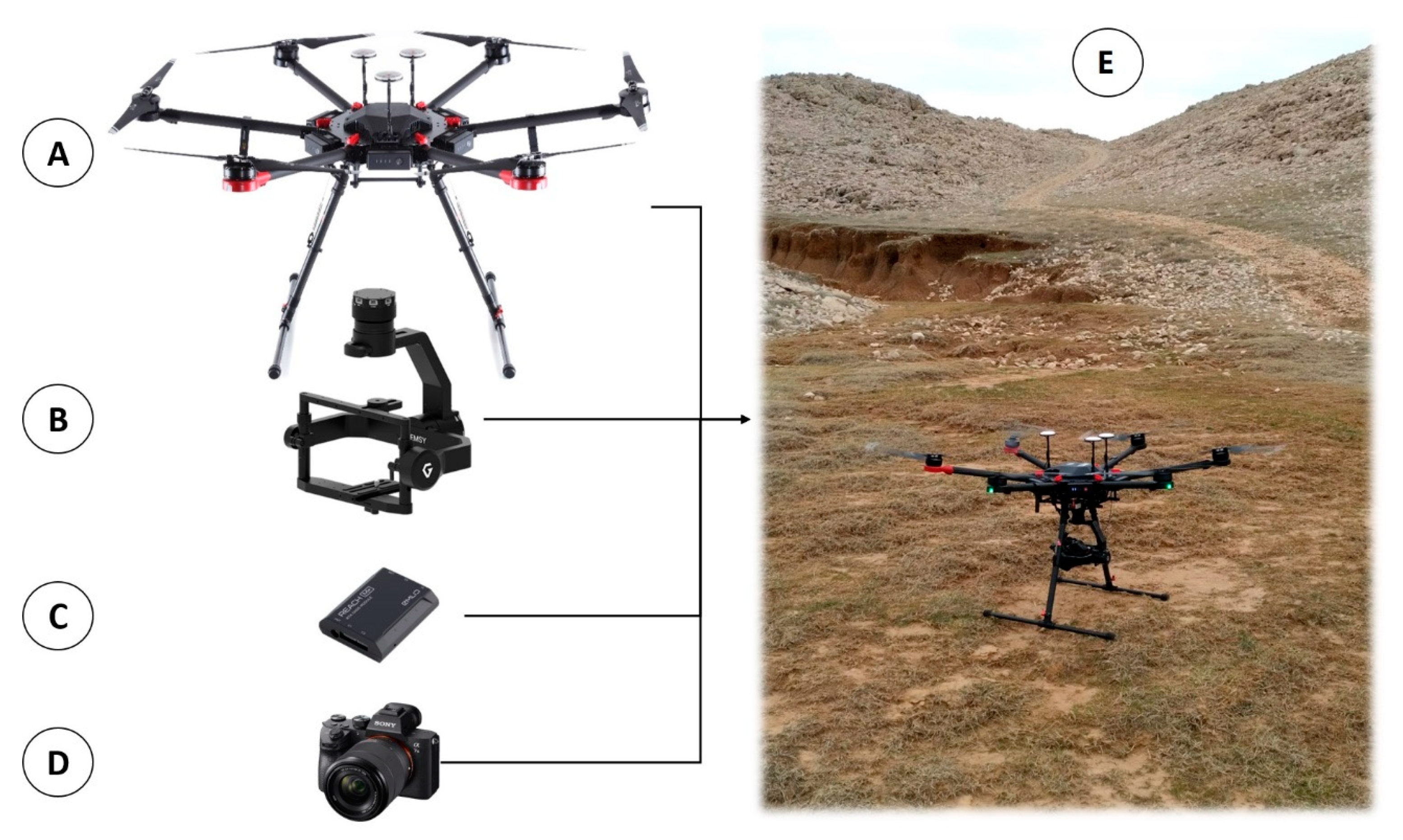
3.1. Assembling and Functional Integration of Repeat Aerophotogrametric System (RAPS)
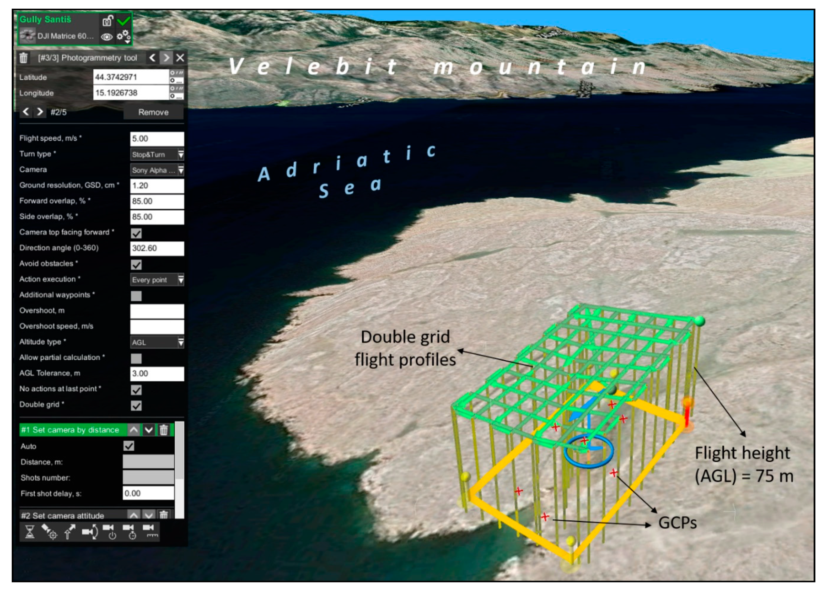
3.2. Field Data Acquisition
3.3. Aerial Data Processing and VHR DSM Creation
Validation of Model Accuracy and Uncertainty
- = minimal level of detection calculated as root sum square of errors based on RMSE values
- = minimal level of detection calculated as root sum square of errors based on MAE values
- = error (RMSE or MAE) for survey A calculated in used CPs
- = error (RMSE or MAE) for survey B calculated in used CPs
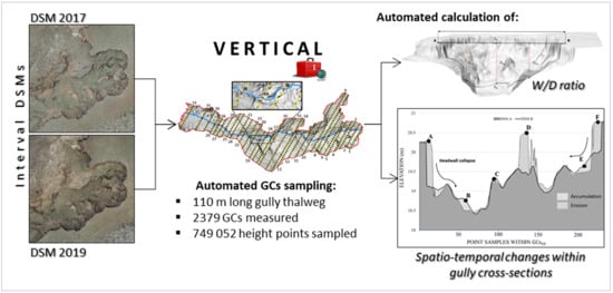
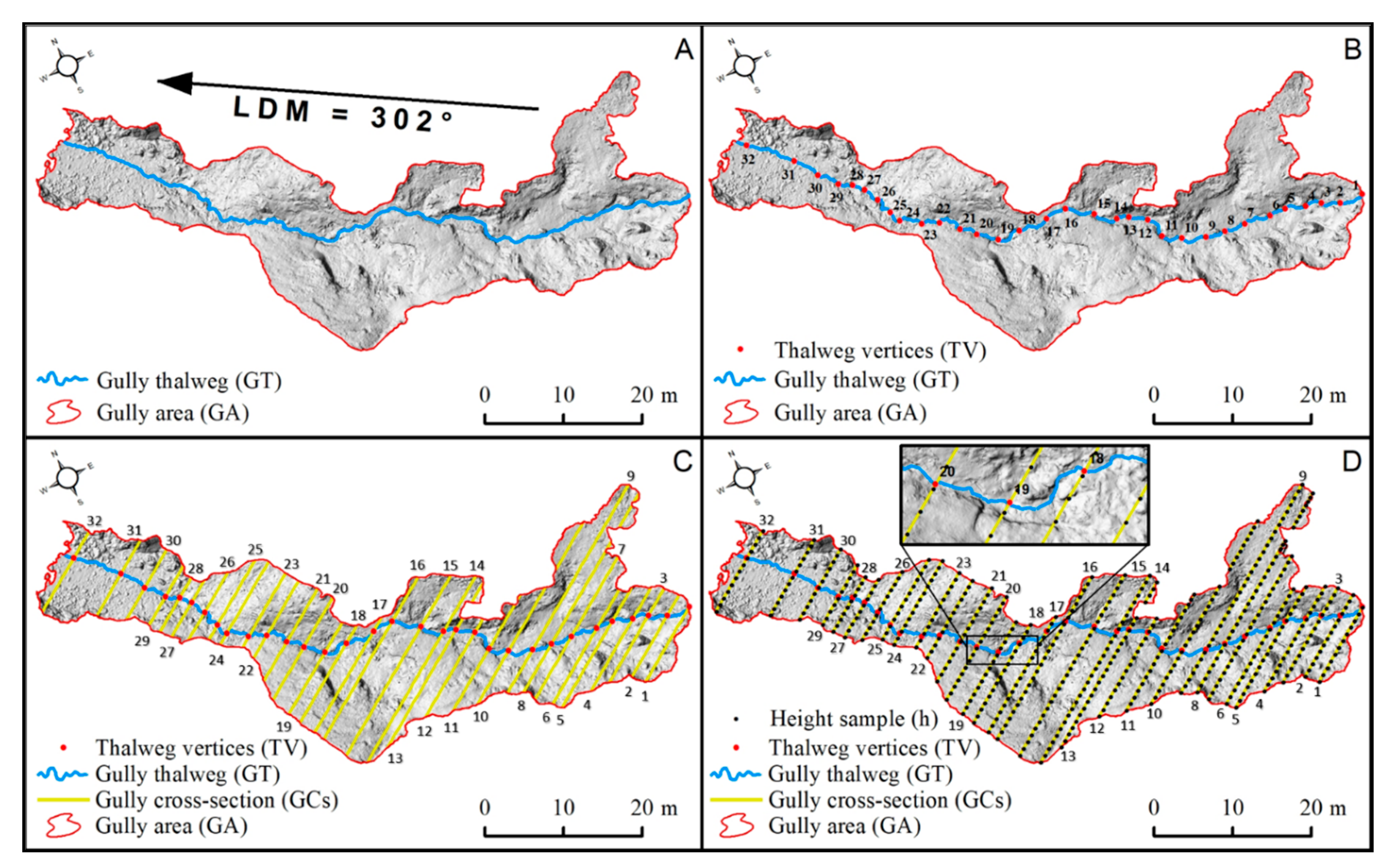
3.4. Development of the VERTICAL Method
- A1 = GCs line constructed left from every MSL vertex
- A2 = GCs line constructed right from every MSL vertex
- LDM = mean linear direction of MSL
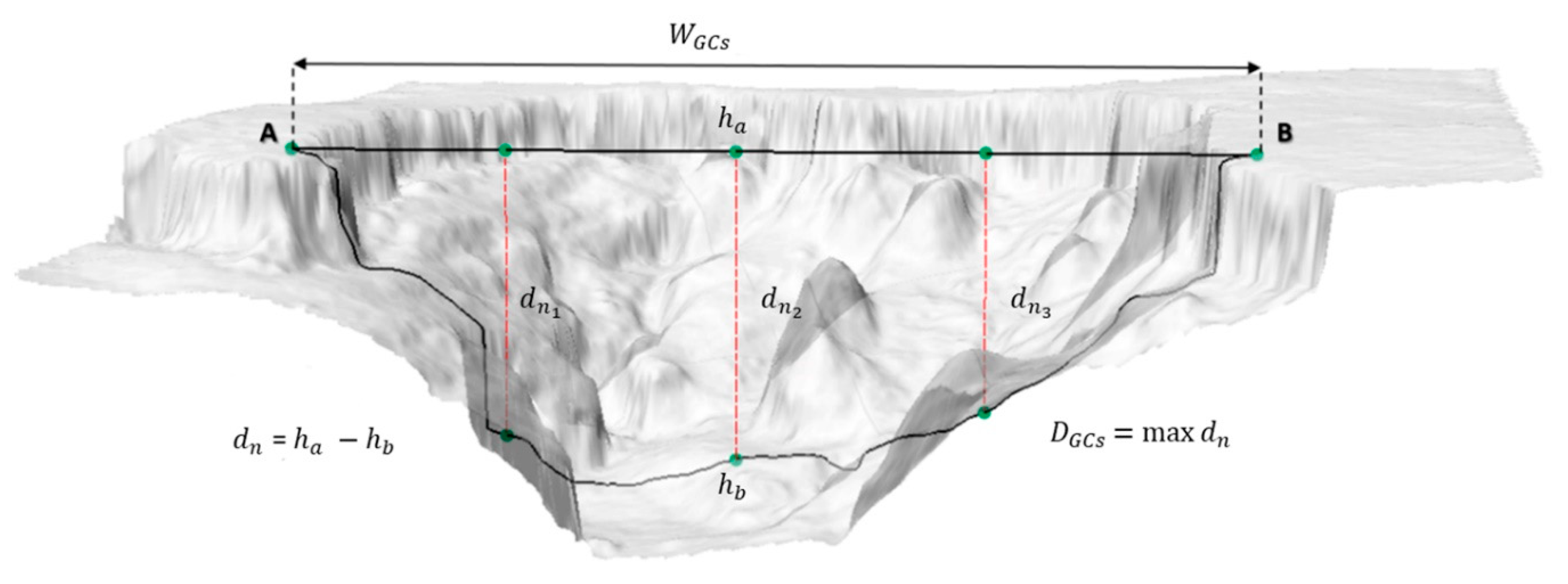
- = height difference at the sampled point
- = height of sampled point in initial DSM
- = height of sampled point in final DSM
- = width of the sampled GCs
- =maximal depth of the sampled GCs
4. Results
4.1. Spatial Resolution and Accuracy of Created Interval VHR Models
4.2. Interpretation of Determined Spatio-Temporal Change
4.3. Interpretation of Derived W/D Ratio
5. Discussion
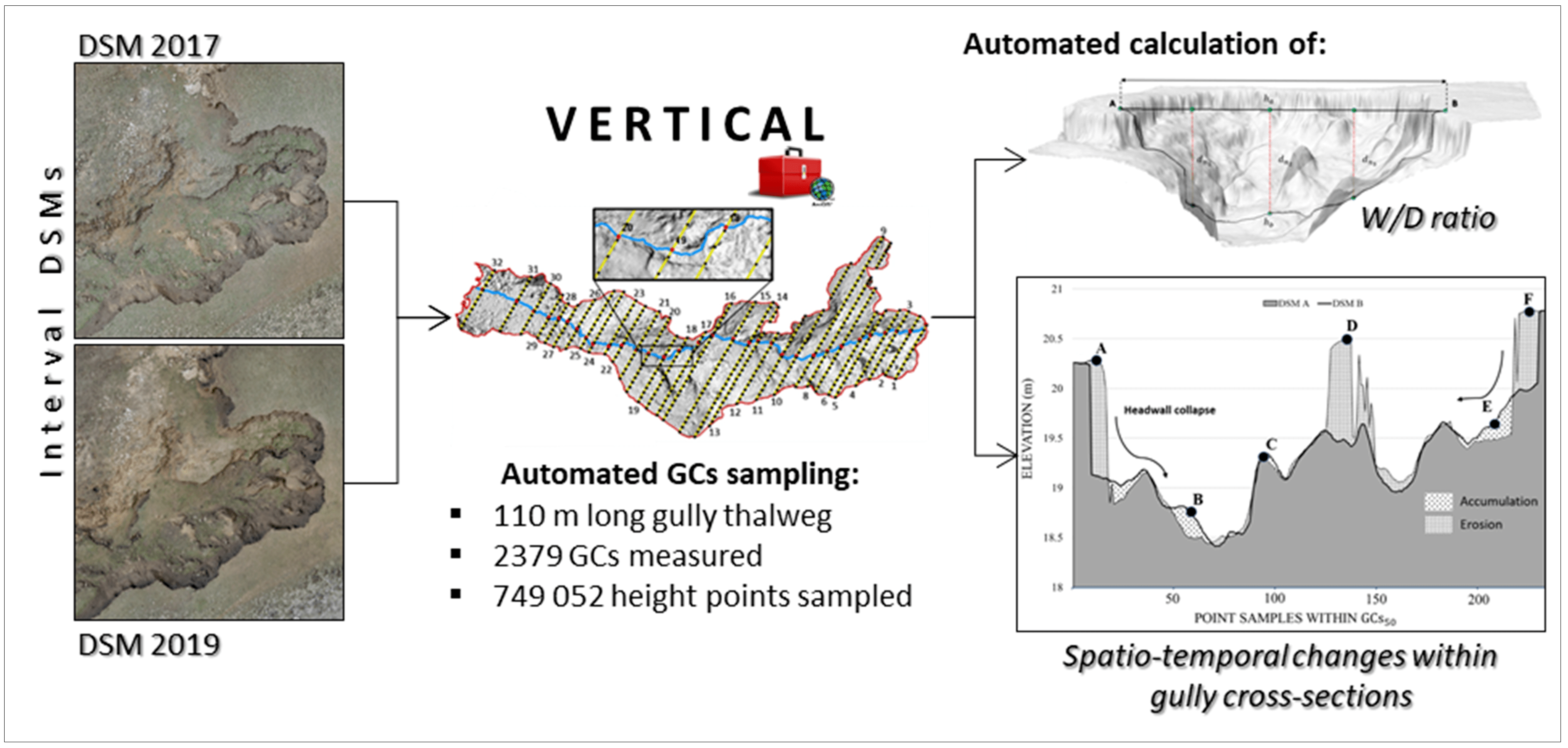
5.1. Advantages of VERTICAL over the Profilometer
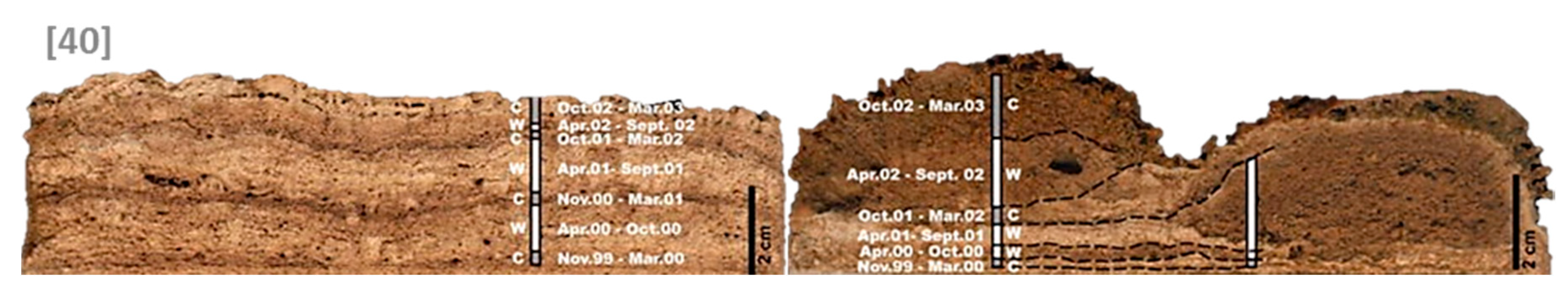
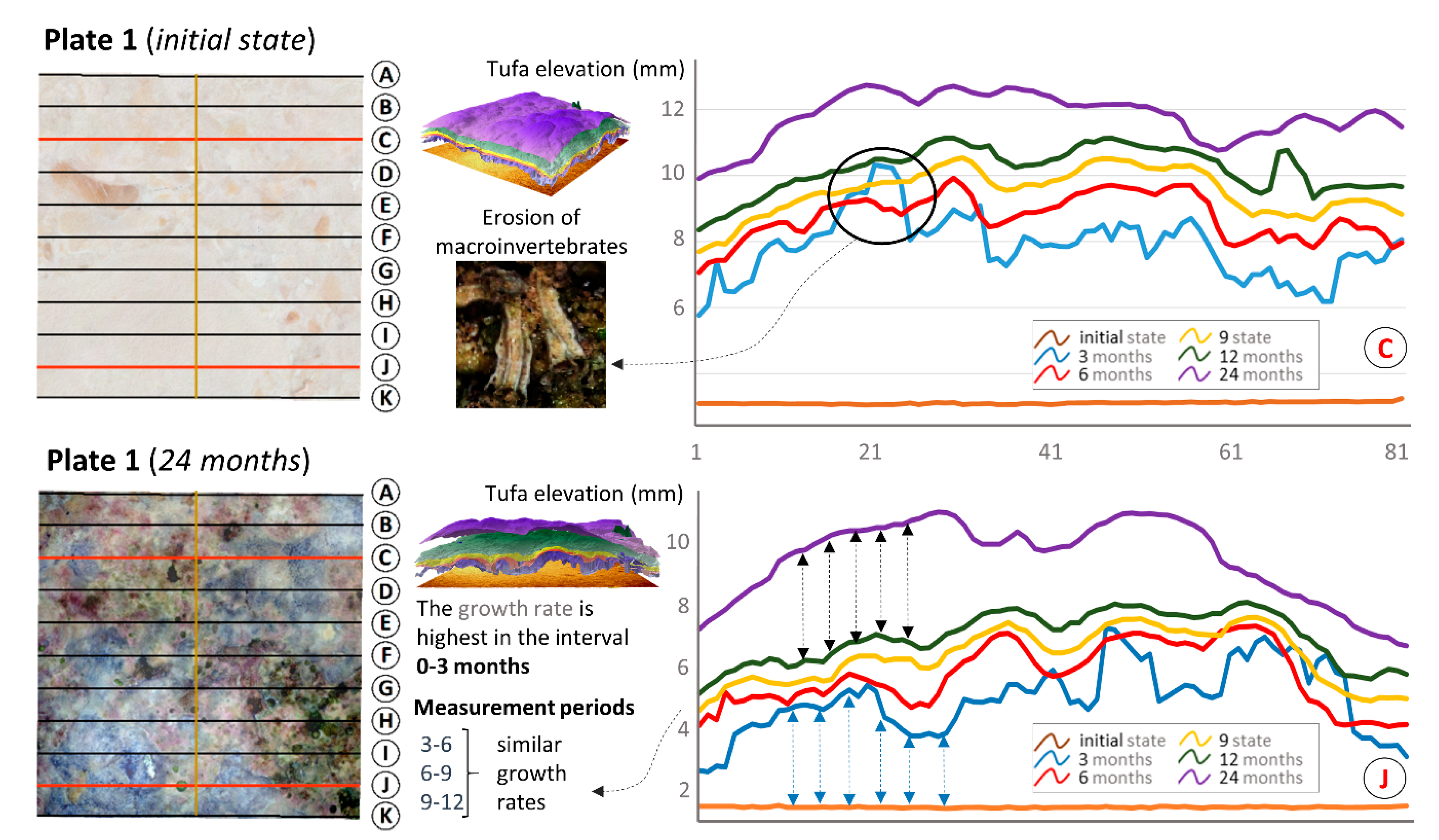
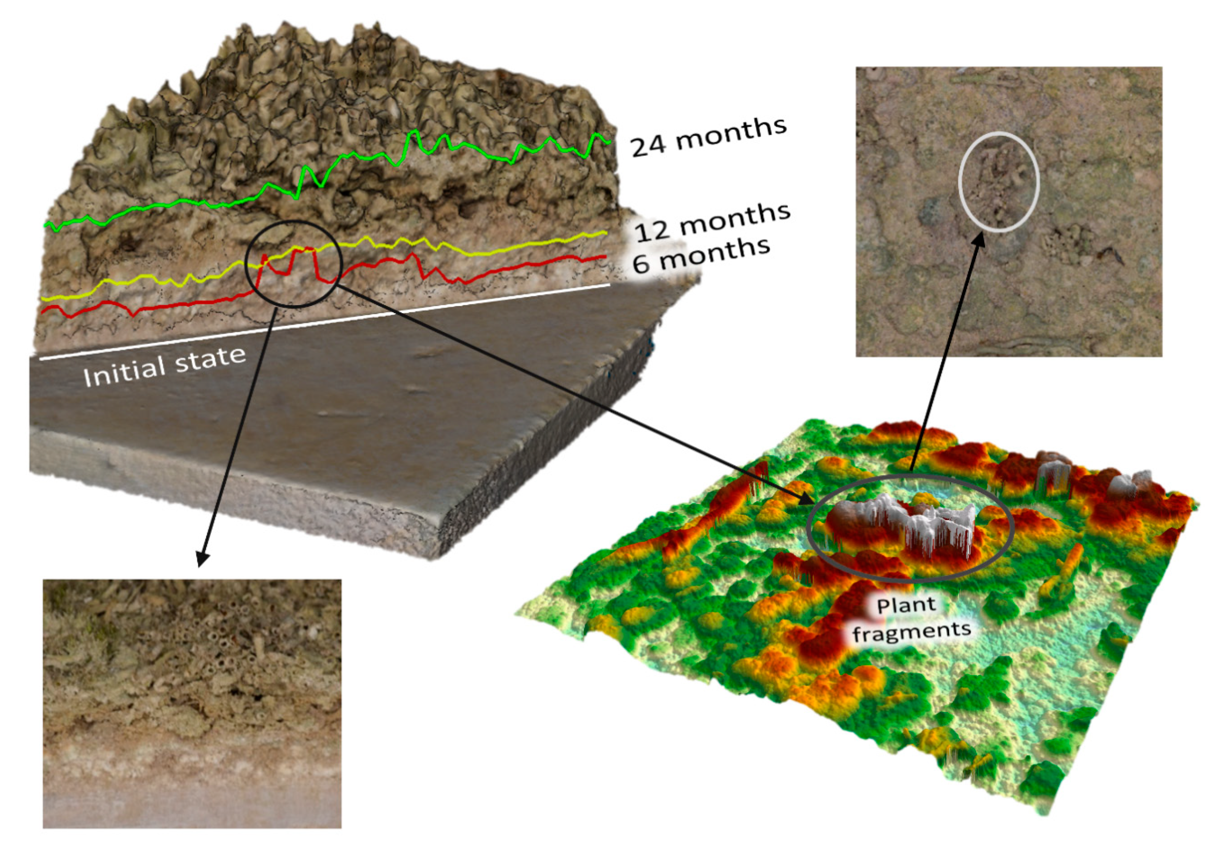
5.2. Applicability of VERTICAL in the Study of Tufa Formation Dynamics (TFD)
5.3. Limitations of VERTICAL Method
6. Conclusions
- (1)
- VERTICAL method successfully overcomes the stated limitations of the profilometer and similar traditional field measurement techniques, as its application facilitates and simplifies the overall process of detection and measurement of vertical spatio-temporal changes within GCs. The extent of the user’s required expertise and its influence on error generation are minimalized with VERTICAL.
- (2)
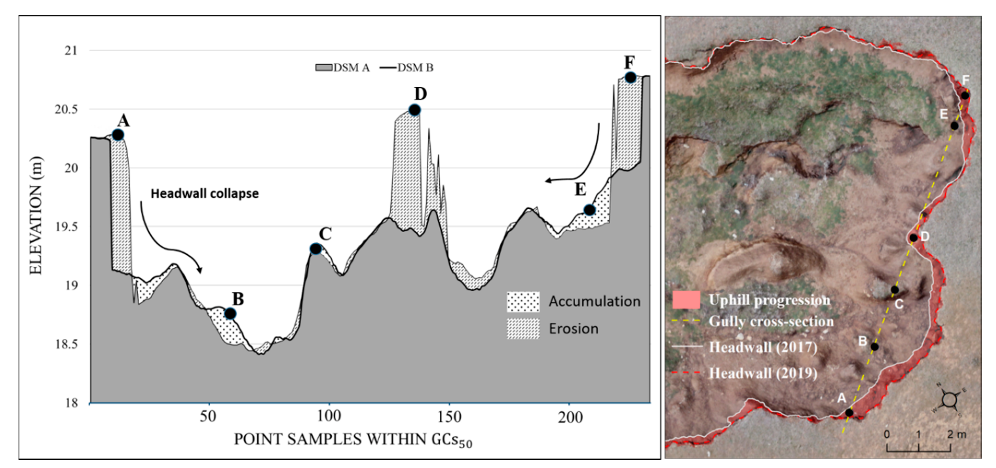
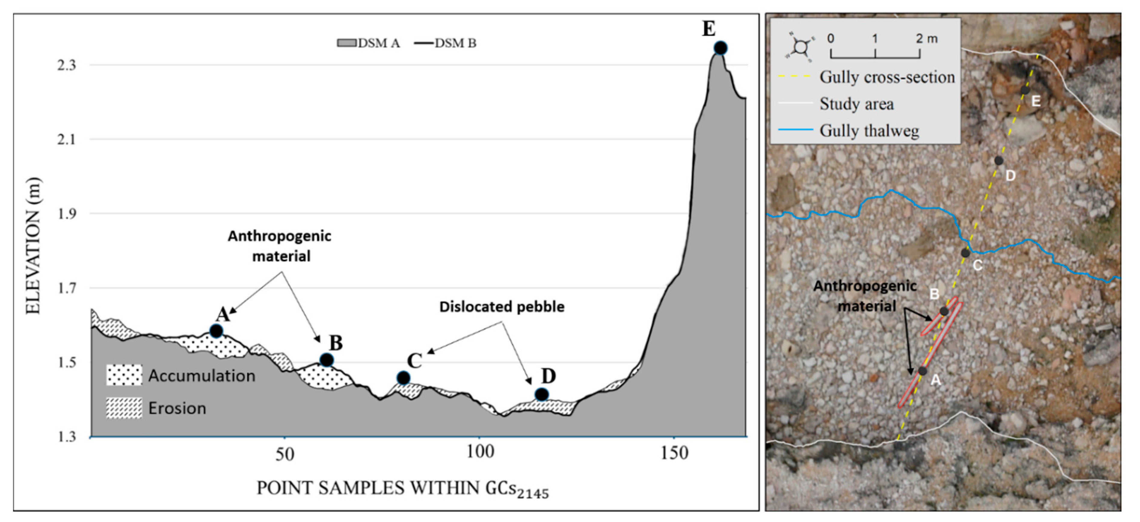
- A very large number of GCs sampled by VERTICAL allows a thorough representation of overall spatio-temporal changes in gully geometry. Due to the high sampling density detailed distinction of different complex erosion and accumulation induced processes is possible. Interpretation of measured spatio-temporal changes is possible within the whole gully (Figure 8), or within separate chosen GCs (Figure 9, Figure 10 and Figure 11).
- (3)
- As demonstrated in Section 5.2, the VERTICAL method is potentially applicable for other, similar scientific purposes, where multi-temporal accurate measurement of spatio-temporal changes in cross-sectional geometry is required (e.g., river material dynamics, ice mass dynamics, tufa sedimentation, and erosion).
- (1)
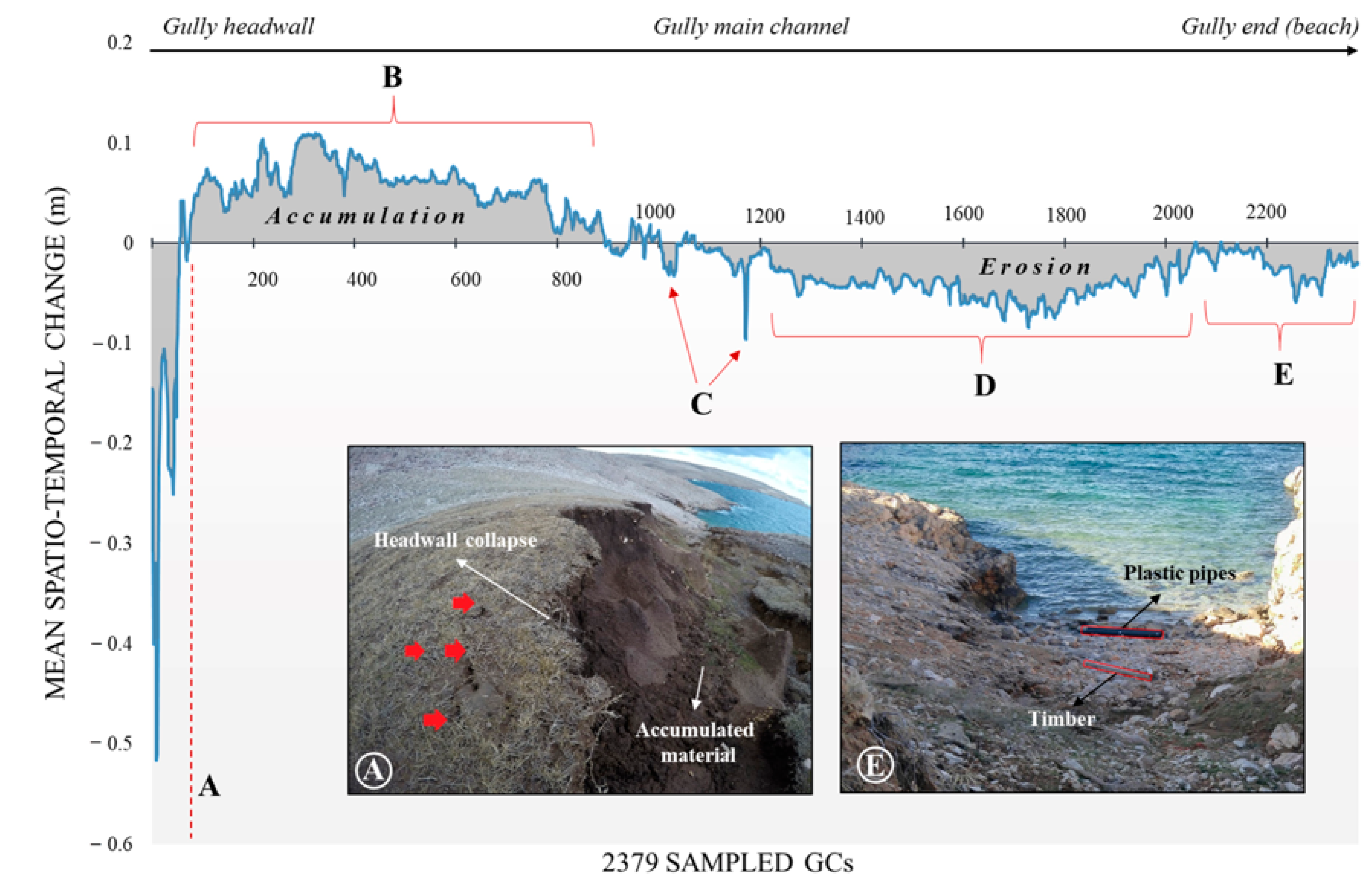
- Mean STC values vary significantly within 2379 GCs of gully Santiš from the gully headcut until the gully terminus.
- (2)
- Highest erosion rates were recorded at the initial part of the gully, where intensive collapse and uphill progression of gully headcut were observed.
- (3)
- Most of the material eroded from gully headcut and sidewalls is being accumulated within the first 20 meters of the gully. Such accumulation could be related to the lack of stronger surface flow, capable of further transportation of eroded material.
- (4)
- Less homogenous middle part of the gully is influenced by the occasional occurrence of stronger selective erosion, manifested mainly through the channel incision and sidewall collapse.
- (5)
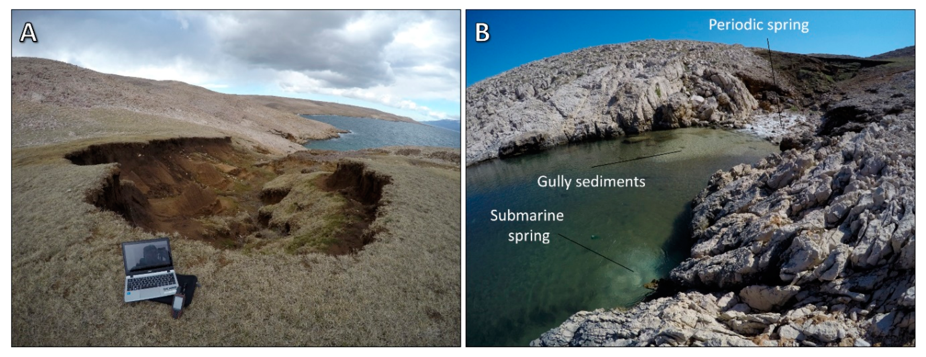
- The final part of gully Santiš is influenced by the dynamics of the Adriatic Sea, which are disrupting and dislocating accumulated sediments.
Supplementary Materials
Author Contributions
Funding
Institutional Review Board Statement
Informed Consent Statement
Data Availability Statement
Acknowledgments
Conflicts of Interest
Abbreviations
| STC | spatio-temporal changes |
| GCs | gully cross-sections |
| VHR | very high resolution |
| UAV | unmanned aerial vehicle |
| RAPS | repeat aerophotogrammetric system |
| GHR | gully headcut retreat |
| SfM | structure from Motion |
| CP | checkpoint |
| GCP | ground control point |
References
- Vandekerckhove, L.; Poesen, J.; Oostwoud-Wijdenes, D.; Nachtergaele, J.; Kosmas, D.; Roxo, M.J.; Figueiredo, T.D. Thresholds for gully initiation and sedimentation in Mediterranean Europe. Earth Surf. Process. Landf. 2000, 25, 1201–1220. [Google Scholar] [CrossRef]
- Wijdenes, D.J.O.; Poesen, J.; Vandekerckhove, L.; Ghesquiere, M. Spatial distribution of gully head activity and sediment supply along an ephemeral channel in a Mediterranean environment. Catena 2000, 39, 147–167. [Google Scholar] [CrossRef]
- Vandekerckhove, L.; Poesen, J.; Wijdenes, D.O.; Gyssels, G. Short-term bank gully retreat rates in Mediterranean environments. Catena 2001, 44, 133–161. [Google Scholar] [CrossRef]
- Vandekerckhove, L.; Poesen, J.; Govers, G. Medium-term gully headcut retreat rates in Southeast Spain determined from aerial photographs and ground measurements. Catena 2003, 50, 329–352. [Google Scholar] [CrossRef]
- Lesschen, J.P.; Kok, K.; Verburg, P.H.; Cammeraat, L.H. Identification of vulnerable areas for gully erosion under different scenarios of land abandonment in Southeast Spain. Catena 2007, 71, 110–121. [Google Scholar] [CrossRef]
- De Baets, S.; Poesen, J.; Reubens, B.; Muys, B.; De Baerdemaeker, J.; Meersmans, J. Methodological framework to select plant species for controlling rill and gully erosion: Application to a Mediterranean ecosystem. Earth Surf. Process. Landf. 2009, 34, 1374–1392. [Google Scholar] [CrossRef]
- Marzolff, I.; Ries, J.B.; Poesen, J. Short-term versus medium-term monitoring for detecting gully-erosion variability in a Mediterranean environment. Earth Surf. Process. Landf. 2011, 36, 1604–1623. [Google Scholar] [CrossRef]
- Ben Slimane, A.; Raclot, D.; Evrard, O.; Sanaa, M.; Lefevre, I.; Le Bissonnais, Y. Relative contribution of rill/interrill and gully/channel erosion to small reservoir siltation in Mediterranean environments. Land Degrad. Dev. 2016, 27, 785–797. [Google Scholar] [CrossRef]
- Erktan, A.; Cécillon, L.; Graf, F.; Roumet, C.; Legout, C.; Rey, F. Increase in soil aggregate stability along a Mediterranean successional gradient in severely eroded gully bed ecosystems: Combined effects of soil, root traits and plant community characteristics. Plant Soil 2016, 398, 121–137. [Google Scholar] [CrossRef]
- Poesen, J.; Nachtergaele, J.; Verstraetena, G.; Valentin, C. Gully erosion and environmental change: Importance and research needs. Catena 2003, 50, 91–133. [Google Scholar] [CrossRef]
- Martínez-Casasnovas, J.A.; Ramos, M.C.; Poesen, J. Assessment of sidewall erosion in large gullies using multi-temporal DEMs and logistic regression analysis. Geomorphology 2004, 58, 305–321. [Google Scholar] [CrossRef]
- Poesen, J.; Vanwalleghem, T.; de Vente, J.; Knapen, A.; Verstraeten, G.; Martínez-Casasnovas, J.A. Gully erosion in Europe. In Soil Erosion in Europe; Boardman, J., Poesen, J., Eds.; John Wiley & Sons: Hoboken, NJ, USA, 2007; pp. 515–536. [Google Scholar]
- Valentin, C.; Poesen, J.; Li, Y. Gully erosion: Impacts, factors and control. Catena 2005, 63, 132–153. [Google Scholar] [CrossRef]
- Herzig, A.; Dymond, J.R.; Marden, M. A gully-complex model for assessing gully stabilisation strategies. Geomorphology 2011, 133, 23–33. [Google Scholar] [CrossRef]
- Vanmaercke, M.; Poesen, J.; Van Mele, B.; Demuzere, M.; Bruynseels, A.; Golosov, V.; Rodrigues Bezerra, J.F.; Bolysov, S.; Dvinskih, A.; Frankl, A.; et al. How fast do gully headcuts retreat? Earth Sci. Rev. 2016, 154, 336–355. [Google Scholar] [CrossRef]
- Gutiérrez, Á.G.; Schnabel, S.; Contador, F.L. Gully erosion, land use and topographical thresholds during the last 60 years in a small rangeland catchment in SW Spain. Land Degrad. Dev. 2009, 20, 535–550. [Google Scholar] [CrossRef]
- Kirkby, M.J.; Bracken, L.J. Gully processes and gully dynamics. Earth Surf. Process. Landf. 2009, 34, 1841–1851. [Google Scholar] [CrossRef]
- Martínez-Casasnovas, J.A.; Ramos, M.C.; García-Hernández, D. Effects of land-use changes in vegetation cover and sidewall erosion in a gully head of the Penedès region (northeast Spain). Earth Surf. Process. Landf. 2009, 34, 1927–1937. [Google Scholar] [CrossRef]
- Campo-Bescós, M.A.; Flores-Cervantes, J.H.; Bras, R.L.; Casalí, J.; Giráldez, J.V. Evaluation of a gully headcut retreat model using multitemporal aerial photographs and digital elevation models. J. Geophys. Res. Earth 2013, 118, 2159–2173. [Google Scholar] [CrossRef] [Green Version]
- Gómez-Gutiérrez, Á.; Schnabel, S.; Berenguer-Sempere, F.; Lavado-Contador, F.; Rubio-Delgado, J. Using 3D photo-reconstruction methods to estimate gully headcut erosion. Catena 2014, 120, 91–101. [Google Scholar] [CrossRef]
- Rengers, F.K.; Tucker, G.E. Analysis and modeling of gully headcut dynamics, North American high plains. J. Geophys. Res. Earth Surf. 2014, 119, 983–1003. [Google Scholar] [CrossRef] [Green Version]
- Giménez, R.; Marzolff, I.; Campo, M.A.; Seeger, M.; Ries, J.B.; Casalí, J.; Alvarez-Mozos, J. Accuracy of high-resolution photogrammetric measurements of gullies with contrasting morphology. Earth Surf. Process. Landf. 2009, 34, 1915–1926. [Google Scholar] [CrossRef]
- Casalí, J.; Giménez, R.; Campo-Bescós, M.A. Gully geometry: What are we measuring? Soil 2015, 1, 509–513. [Google Scholar] [CrossRef] [Green Version]
- Deng, Q.; Qin, F.; Zhang, B.; Wang, H.; Luo, M.; Shu, C.; Liu, H.; Liu, G. Characterizing the morphology of gully cross-sections based on PCA: A case of Yuanmou Dry-Hot Valley. Geomorphology 2015, 228, 703–713. [Google Scholar] [CrossRef]
- Feng, Y.; Mu, H.; Qin, F.; Deng, Q.; Liu, H.; Zhang, B.; Liu, S.; Liu, G. Modeling the morphology of gully cross sections in the Yuanmou Dry-hot Valley. Phys. Geogr. 2017, 38, 448–469. [Google Scholar] [CrossRef]
- Casalí, J.; Loizu, J.; Campo, M.A.; De Santisteban, L.M.; Álvarez-Mozos, J. Accuracy of methods for field assessment of rill and ephemeral gully erosion. Catena 2006, 67, 128–138. [Google Scholar] [CrossRef]
- Castillo, C.; Pérez, R.; James, M.R.; Quinton, J.N.; Taguas, E.V.; Gómez, J.A. Comparing the accuracy of several field methods for measuring gully erosion. Soil Sci. Soc. Am. J. 2012, 76, 1319–1332. [Google Scholar] [CrossRef] [Green Version]
- Moges, A.; Holden, N.M. Estimating the rate and consequences of gully development, a case study of Umbulo catchment in southern Ethiopia. Land Degrad. Dev. 2008, 19, 574–586. [Google Scholar] [CrossRef]
- Zheng, F.; Wackrow, R.; Meng, F.R.; Lobb, D.; Li, S. Assessing the Accuracy and Feasibility of Using Close-Range Photogrammetry to Measure Channelized Erosion with a Consumer-Grade Camera. Remote Sens. 2020, 12, 1706. [Google Scholar] [CrossRef]
- Caraballo-Arias, N.A.; Conoscenti, C.; Di Stefano, C.; Ferro, V.; Gómez-Gutiérrez, A. Morphometric and hydraulic geometry assessment of a gully in SW Spain. Geomorphology 2016, 274, 143–151. [Google Scholar] [CrossRef] [Green Version]
- Casalí, J.; López, J.J.; Giráldez, J.V. Ephemeral gully erosion in southern Navarra (Spain). Catena 1999, 36, 65–84. [Google Scholar] [CrossRef]
- Capra, A.; Di Stefano, C.; Ferro, V.; Scicolone, B. Similarity between morphological characteristics of rills and ephemeral gullies in Sicily, Italy. Hydrol. Process. Int. J. 2009, 23, 3334–3341. [Google Scholar] [CrossRef]
- Perez-Gutierrez, C.; Álvarez-Mozos, J.; Martínez-Fernández, J.; Sánchez, N. Comparison of a multilateral-based acquisition with Terrestrial Laser Scanner and profilometer technique for soil roughness measurement. In Proceedings of the 2010 IEEE International Geoscience and Remote Sensing Symposium, Honolulu, HI, USA, 25–30 July 2010; pp. 2988–2991. [Google Scholar]
- Álvarez-Mozos, J.; Campo, M.Á.; Giménez, R.; Casalí, J.; Leibar, U. Implications of scale, slope, tillage operation and direction in the estimation of surface depression storage. Soil Tillage Res. 2011, 111, 142–153. [Google Scholar] [CrossRef]
- Perroy, R.L.; Bookhagen, B.; Asner, G.P.; Chadwick, O.A. Comparison of gully erosion estimates using airborne and ground-based LiDAR on Santa Cruz Island, California. Geomorphology 2010, 118, 288–300. [Google Scholar] [CrossRef]
- Whitford, J.A.; Newham, L.T.H.; Vigiak, O.; Melland, A.R.; Roberts, A.M. Rapid assessment of gully sidewall erosion rates in data-poor catchments: A case study in Australia. Geomorphology 2010, 118, 330–338. [Google Scholar] [CrossRef]
- Marić, I.; Šiljeg, A.; Cukrov, N.; Roland, V.; Domazetović, F. How fast does tufa grow? Very high-resolution measurement of the tufa growth rate on artificial substrates by the development of a contactless image-based modelling device. Earth Surf. Process. Landf. 2020, 45, 2331–2349. [Google Scholar] [CrossRef]
- Marzolff, I.; Poesen, J. The potential of 3D gully monitoring with GIS using high-resolution aerial photography and a digital photogrammetry system. Geomorphology 2009, 111, 48–60. [Google Scholar] [CrossRef]
- Pike, A.; Mueller, T.; Rienzi, E.; Neelakantan, S.; Mijatovic, B.; Karathanasis, T.; Rodrigues, M. Terrain Analysis for Locating Erosion Channels: Assessing LiDAR Data and Flow Direction Algorithm. Plant Soil Sci. Fac. Publ. 2012, 51, 45–63. [Google Scholar]
- Stöcker, C.; Eltner, A.; Karrasch, P. Measuring gullies by synergetic application of UAV and close range photogrammetry—A case study from Andalusia, Spain. Catena 2015, 132, 1–11. [Google Scholar] [CrossRef]
- Viles, H. Technology and geomorphology: Are improvements in data collection techniques transforming geomorphic science? Geomorphology 2016, 270, 121–133. [Google Scholar] [CrossRef]
- Westoby, M.J.; Brasington, J.; Glasser, N.F.; Hambrey, M.J.; Reynolds, J.M. ‘Structure-from-Motion’photogrammetry: A low-cost, effective tool for geoscience applications. Geomorphology 2012, 179, 300–314. [Google Scholar] [CrossRef] [Green Version]
- Clapuyt, F.; Vanacker, V.; Van Oost, K. Reproducibility of UAV-based earth topography reconstructions based on Structure-from-Motion algorithms. Geomorphology 2016, 260, 4–15. [Google Scholar] [CrossRef]
- Eltner, A.; Kaiser, A.; Castillo, C.; Rock, G.; Neugirg, F.; Abellán, A. Image-based surface reconstruction in geomorphometry–merits, limits and developments. Earth Surf. Dyn. 2016, 4, 359–389. [Google Scholar] [CrossRef] [Green Version]
- James, M.R.; Robson, S.; d’Oleire-Oltmanns, S.; Niethammer, U. Optimising UAV topographic surveys processed with structure-from-motion: Ground control quality, quantity and bundle adjustment. Geomorphology 2017, 280, 51–66. [Google Scholar] [CrossRef] [Green Version]
- Mosbrucker, A.R.; Major, J.J.; Spicer, K.R.; Pitlick, J. Camera system considerations for geomorphic applications of SfM photogrammetry. Earth Surf. Process. Landf. 2017, 42, 969–986. [Google Scholar] [CrossRef] [Green Version]
- Kasprzak, M.; Jancewicz, K.; Michniewicz, A. UAV and SfM in detailed geomorphological mapping of granite tors: An example of Starościńskie Skały (Sudetes, SW Poland). Pure Appl. Geophys. 2018, 175, 3193–3207. [Google Scholar] [CrossRef] [Green Version]
- Gomez, C.; Hayakawa, Y.; Obanawa, H. A study of Japanese landscapes using structure from motion derived DSMs and DEMs based on historical aerial photographs: New opportunities for vegetation monitoring and diachronic geomorphology. Geomorphology 2015, 242, 11–20. [Google Scholar] [CrossRef] [Green Version]
- Dietrich, J.T. Applications of Structure-from-Motion Photogrammetry to Fluvial Geomorphology. Ph.D. Thesis, University of Oregon, Eugene, OR, USA, December 2014. Available online: https://0-search-proquest-com.brum.beds.ac.uk/openview/c62ca57d49fed676ce963409dc53cfad/1?pq-origsite=gscholar&cbl=18750&diss=y (accessed on 14 February 2020).
- Ewertowski, M.W.; Tomczyk, A.M.; Evans, D.J.; Roberts, D.H.; Ewertowski, W. Operational framework for rapid, very-high resolution mapping of glacial geomorphology using low-cost unmanned aerial vehicles and structure-from-motion approach. Remote Sens. 2019, 11, 65. [Google Scholar] [CrossRef] [Green Version]
- Meinen, B.U.; Robinson, D.T. Where did the soil go? Quantifying one year of soil erosion on a steep tile-drained agricultural field. Sci. Total Environ. 2020, 729, 138320. [Google Scholar] [CrossRef]
- Meinen, B.U.; Robinson, D.T. Mapping erosion and deposition in an agricultural landscape: Optimization of UAV image acquisition schemes for SfM-MVS. Remote Sens. Environ. 2020, 239, 111666. [Google Scholar] [CrossRef]
- Gong, C.; Lei, S.; Bian, Z.; Liu, Y.; Zhang, Z.; Cheng, W. Analysis of the Development of an Erosion Gully in an Open-Pit Coal Mine Dump During a Winter Freeze-Thaw Cycle by Using Low-Cost UAVs. Remote Sens. 2019, 11, 1356. [Google Scholar] [CrossRef] [Green Version]
- Hemmelder, S.; Marra, W.; Markies, H.; De Jong, S.M. Monitoring river morphology & bank erosion using UAV imagery–A case study of the river Buëch, Hautes-Alpes, France. Int. J. Appl. Earth Obs. Geoinf. 2018, 73, 428–437. [Google Scholar]
- Glendell, M.; McShane, G.; Farrow, L.; James, M.R.; Quinton, J.; Anderson, K.; Evans, M.; Benaud, P.; Rawlins, B.; Morgan, D.; et al. Testing the utility of structure-from-motion photogrammetry reconstructions using small unmanned aerial vehicles and ground photography to estimate the extent of upland soil erosion. Earth Surf. Process. Landf. 2017, 42, 1860–1871. [Google Scholar] [CrossRef]
- Pineux, N.; Lisein, J.; Swerts, G.; Bielders, C.L.; Lejeune, P.; Colinet, G.; Degré, A. Can DEM time series produced by UAV be used to quantify diffuse erosion in an agricultural watershed? Geomorphology 2017, 280, 122–136. [Google Scholar] [CrossRef]
- Neugirg, F.; Stark, M.; Kaiser, A.; Vlacilova, M.; Della Seta, M.; Vergari, F.; Schmidt, J.; Becht, M.; Haas, F. Erosion processes in calanchi in the Upper Orcia Valley, Southern Tuscany, Italy based on multitemporal high-resolution terrestrial LiDAR and UAV surveys. Geomorphology 2016, 269, 8–22. [Google Scholar] [CrossRef]
- Carollo, F.G.; Di Stefano, C.; Ferro, V.; Pampalone, V. Measuring rill erosion at plot scale by a drone-based technology. Hydrol. Process. 2015, 29, 3802–3811. [Google Scholar] [CrossRef]
- Bazzoffi, P. Measurement of rill erosion through a new UAV-GIS methodology. Ital. J. Agron. 2015, 10, 708. [Google Scholar] [CrossRef] [Green Version]
- Kaiser, A.; Neugirg, F.; Rock, G.; Müller, C.; Haas, F.; Ries, J.; Schmidt, J. Small-scale surface reconstruction and volume calculation of soil erosion in complex Moroccan gully morphology using structure from motion. Remote Sens. 2014, 6, 7050–7080. [Google Scholar] [CrossRef] [Green Version]
- Hayakawa, Y.S.; Obanawa, H. Volumetric change detection in bedrock coastal cliffs using terrestrial laser scanning and uas-based SFM. Sensors 2020, 20, 3403. [Google Scholar] [CrossRef]
- Koutalakis, P.; Tzoraki, O.; Gkiatas, G.; Zaimes, G.N. Using UAV to Capture and Record Torrent Bed and Banks, Flood Debris, and Riparian Areas. Drones 2020, 4, 77. [Google Scholar] [CrossRef]
- Cucchiaro, S.; Fallu, D.J.; Zhang, H.; Walsh, K.; Van Oost, K.; Brown, A.G.; Tarolli, P. Multiplatform-SfM and TLS data fusion for monitoring agricultural terraces in complex topographic and landcover conditions. Remote Sens. 2020, 12, 1946. [Google Scholar] [CrossRef]
- Hout, R.; Maleval, V.; Mahe, G.; Rouvellac, E.; Crouzevialle, R.; Cerbelaud, F. UAV and LiDAR Data in the Service of Bank Gully Erosion Measurement in Rambla de Algeciras Lakeshore. Water 2020, 12, 2748. [Google Scholar] [CrossRef]
- D’Oleire-Oltmanns, S.; Marzolff, I.; Peter, K.D.; Ries, J.B. Unmanned aerial vehicle (UAV) for monitoring soil erosion in Morocco. Remote Sens. 2012, 4, 3390–3416. [Google Scholar] [CrossRef] [Green Version]
- Frankl, A.; Stal, C.; Abraha, A.; Nyssen, J.; Rieke-Zapp, D.; De Wulf, A.; Poesen, J. Detailed recording of gully morphology in 3D through image-based modelling. Catena 2015, 127, 92–101. [Google Scholar] [CrossRef] [Green Version]
- Li, Z.; Zhang, Y.; Zhu, Q.; Yang, S.; Li, H.; Ma, H. A gully erosion assessment model for the Chinese Loess Plateau based on changes in gully length and area. Catena 2017, 148, 195–203. [Google Scholar] [CrossRef]
- Castillo, C.; Marín-Moreno, V.J.; Pérez, R.; Muñoz-Salinas, R.; Taguas, E.V. Accurate automated assessment of gully cross-section geometry using the photogrammetric interface FreeXSapp. Earth Surf. Process. Landf. 2018, 43, 1726–1736. [Google Scholar] [CrossRef]
- Wu, H.; Xu, X.; Zheng, F.; Qin, C.; He, X. Gully morphological characteristics in the loess hilly-gully region based on 3D laser scanning technique. Earth Surf. Process. Landf. 2018, 43, 1701–1710. [Google Scholar] [CrossRef]
- Castillo, C.; Campo-Bescós, M.A.; Giménez, R.; Pérez, R.; Casalí, J. The Optimal Lid Method for the objective definition of cross-section limits in ephemeral gullies. Catena 2019, 176, 381–393. [Google Scholar] [CrossRef]
- Frankl, A.; Poesen, J.; Scholiers, N.; Jacob, M.; Haile, M.; Deckers, J.; Nyssen, J. Factors controlling the morphology and volume (V)–length (L) relations of permanent gullies in the northern Ethiopian Highlands. Earth Surf. Process. Landf. 2013, 38, 1672–1684. [Google Scholar] [CrossRef] [Green Version]
- Heede, B.H. Morphology of gullies in the Colorado Rocky Mountains. Hydrol. Sci. J. 1970, 15, 79–89. [Google Scholar] [CrossRef]
- Tuckfield, C. Gully erosion in New Forest Hampshire. Am. J. Sci. 1964, 262, 795–807. [Google Scholar] [CrossRef]
- Poesen, J.; Govers, G. Gully erosion in the loam belt of Belgium: Typology and control measures. In Soil Erosion on Agricultural Land; Boardman, J., Foster, I.D.L., Dearing, J.A., Eds.; John Wiley & Sons Ltd.: Coventry, UK, 1989; pp. 513–530. [Google Scholar]
- Blong, R.J.; Graham, O.P.; Veness, J.A. The role of sidewall processes in gully development; some NSW examples. Earth Surf. Process. Landf. 1982, 7, 381–385. [Google Scholar] [CrossRef]
- Crouch, R.J. The relationship of gully sidewall shape to sediment production. Soil Res. 1987, 25, 531–539. [Google Scholar] [CrossRef]
- Gabet, E.J.; Bookter, A. A morphometric analysis of gullies scoured by post-fire progressively bulked debris flows in southwest Montana, USA. Geomorphology 2008, 96, 298–309. [Google Scholar] [CrossRef]
- Joshi, V.U. Soil loss estimation by field measurements in the badlands along Pravara river (Western India). J. Geol. Soc. India 2014, 83, 613–624. [Google Scholar] [CrossRef]
- Vinci, A.; Brigante, R.; Todisco, F.; Mannocchi, F.; Radicioni, F. Measuring rill erosion by laser scanning. Catena 2015, 124, 97–108. [Google Scholar] [CrossRef]
- Loughran, R.J. The measurement of soil erosion. Prog. Phys. Geogr. 1989, 13, 216–233. [Google Scholar] [CrossRef]
- Kornecki, T.S.; Fouss, J.L.; Prior, S.A. A portable device to measure soil erosion/deposition in quarter-drains. Soil Use Manag. 2008, 24, 401–408. [Google Scholar] [CrossRef]
- Sirvent, J.; Desir, G.; Gutierrez, M.; Sancho, C.; Benito, G. Erosion rates in badland areas recorded by collectors, erosion pins and profilometer techniques (Ebro Basin, NE-Spain). Geomorphology 1997, 18, 61–75. [Google Scholar] [CrossRef]
- Ryan, J.C.; Hubbard, A.L.; Todd, J.; Carr, J.R.; Box, J.E.; Christoffersen, P.; Holt, T.O.; Snooke, N. Repeat UAV photogrammetry to assess calving front dynamics at a large outlet glacier draining the Greenland Ice Sheet. Cryosphere Discuss 2014, 8, 2243–2275. [Google Scholar] [CrossRef] [Green Version]
- Dewez, T.; Leroux, J.; Morelli, S. Cliff collapse hazard from repeated multicopter UAV acquisitions: Return on experience. In Proceedings of the XXIII ISPRS Congress, Prague, Czech Republic, 12–19 July 2016; pp. 805–811. [Google Scholar]
- Rossini, M.; Di Mauro, B.; Garzonio, R.; Baccolo, G.; Cavallini, G.; Mattavelli, M.; De Amicis, M.; Colombo, R. Rapid melting dynamics of an alpine glacier with repeated UAV photogrammetry. Geomorphology 2018, 304, 159–172. [Google Scholar] [CrossRef]
- Ajayi, O.G.; Salubi, A.A.; Angbas, A.F.; Odigure, M.G. Generation of accurate digital elevation models from UAV acquired low percentage overlapping images. Int. J. Remote Sens. 2017, 38, 3113–3134. [Google Scholar] [CrossRef]
- Cook, K.L. An evaluation of the effectiveness of low-cost UAVs and structure from motion for geomorphic change detection. Geomorphology 2017, 278, 195–208. [Google Scholar] [CrossRef]
- Koci, J.; Jarihani, B.; Leon, J.X.; Sidle, R.; Wilkinson, S.; Bartley, R. Assessment of UAV and ground-based structure from motion with multi-view stereo photogrammetry in a gullied savanna catchment. ISPRS Int. J. Geo-Inf. 2017, 6, 328. [Google Scholar] [CrossRef] [Green Version]
- Lončar, N. Geomorphologic regionalization of the central and southern parts of Pag Island. Geoadria 2009, 14, 5–25. [Google Scholar] [CrossRef]
- Domazetović, F.; Šiljeg, A.; Lončar, N.; Marić, I. Development of automated multicriteria GIS analysis of gully erosion susceptibility. Appl. Geogr. 2019, 112, 102083. [Google Scholar] [CrossRef]
- Faivre, S.; Pahernik, M.; Maradin, M. The gully of Potovošća on the Island of Krk—He effects of short-term rainfall event. Geol. Croat. 2011, 64, 67–80. [Google Scholar] [CrossRef]
- Castillo, C.; Gómez, J.A. A century of gully erosion research: Urgency, complexity and study approaches. Earth Sci. Rev. 2016, 160, 300–319. [Google Scholar] [CrossRef]
- Domazetović, F.; Šiljeg, A.; Lončar, N.; Marić, I. GIS automated multicriteria analysis (GAMA) method for susceptibility modelling. MethodsX 2019, 6, 2553–2561. [Google Scholar] [CrossRef]
- Mamužić, P.; Sokač, B. Osnovna Geološka Karta SFRJ 1:100 000. Tumač za Listove Silba L 33-126 i Molat L 33-138; Institut za geološka istraživanja: Zagreb, Croatia; Savezni geološki zavod: Beograd, Serbia, 1973; p. 45. [Google Scholar]
- Sokač, B.; Šćavničar, B.; Velić, I. Osnovna Geološka Karta SFRJ 1:100 000. Tumač za List GospićL 33-127; Institut za geološka istraživanja: Zagreb, Croatia; Savezni geološki zavod: Beograd, Serbia, 1976; p. 64. [Google Scholar]
- Zaninović, K.; Gajić-Čapka, M.; Tadić, M.P.; Vučetić, M.; Milković, J.; Bajić, A.; Cindrić, K.; Cvitan, L.; Katušin, Z.; Kaučić, D.; et al. Climate atlas of Croatia: 1961–1990: 1971–2000; Croatian Meteorological and Hydrological Service: Zagreb, Croatia, 2008. [Google Scholar]
- CMHS. Croatian Meteorological and Hydrological Service; Station Pag; Croatian Meteorological and Hydrological Service: Zagreb, Croatia, 2017. [Google Scholar]
- Bašić, F. The soils of Croatia; Springer: Dordrecht, The Netherlands; Heidelberg, Germany; New York, NY, USA; London, UK, 2014. [Google Scholar]
- DJI. Matrice 600 PRO—Simply Professional Performance. 2019. Available online: https://www.dji.com/hr/matrice600-pro (accessed on 23 July 2019).
- Gremsy. T3—Let Your Creativity Run Free. 2019. Available online: https://gremsy.com/gremsy-t3/ (accessed on 12 September 2019).
- Emlid. RTK GNSS Modules for UAV Mapping. 2019. Available online: https://emlid.com/reach/#reach-mapping (accessed on 12 September 2019).
- UgCS. Leading Drone Control Software to Elevate Your Productivity. 2019. Available online: https://www.ugcs.com/ (accessed on 4 March 2019).
- Oniga, V.E.; Breaban, A.I.; Statescu, F. Determining the optimum number of ground control points for obtaining high precision results based on UAS images. Proceedings 2018, 2, 352. [Google Scholar] [CrossRef] [Green Version]
- Stonex. S10 GNSS Receiver-Datasheet. 2019. Available online: http://www.stonex.hr/S10.pdf (accessed on 14 July 2019).
- Gini, R.; Pagliari, D.; Passoni, D.; Pinto, L.; Sona, G.; Dosso, P. UAV photogrammetry: Block triangulation comparisons. Int. Arch. Photogram. Remote Sens. Spat. Inf. Sci. 2014, 1, W2. [Google Scholar] [CrossRef] [Green Version]
- Mancini, F.; Dubbini, M.; Gattelli, M.; Stecchi, F.; Fabbri, S.; Gabbianelli, G. Using unmanned aerial vehicles (UAV) for high-resolution reconstruction of topography: The structure from motion approach on coastal environments. Remote Sens. 2013, 5, 6880–6898. [Google Scholar] [CrossRef] [Green Version]
- Agisoft. Agisoft Metashape User Manual Professional Edition, Version 1.6. 2019. Available online: https://www.agisoft.com/pdf/metashape-pro_1_6_en.pdf (accessed on 14 July 2019).
- James, M.R.; Chandler, J.H.; Eltner, A.; Fraser, C.; Miller, P.E.; Mills, J.P.; Noble, T.; Robson, S.; Lane, S.N. Guidelines on the use of structure-from-motion photogrammetry in geomorphic research. Earth Surf. Process. Landf. 2019, 44, 2081–2084. [Google Scholar] [CrossRef]
- Neverman, A.J.; Fuller, I.C.; Procter, J.N. Application of geomorphic change detection (GCD) to quantify morphological budgeting error in a New Zealand gravel-bed river: A case study from the Makaroro river, Hawke’s bay. J. Hydrol. 2016, 55, 45–63. [Google Scholar]
- Fernández, T.; Pérez, J.L.; Colomo, C.; Cardenal, J.; Delgado, J.; Palenzuela, J.A.; Palenzuela, J.A.; Irigaray, C.; Chacón, J. Assessment of the evolution of a landslide using digital photogrammetry and LiDAR techniques in the Alpujarras region (Granada, southeastern Spain). Geosciences 2017, 7, 32. [Google Scholar] [CrossRef] [Green Version]
- Bates, C.B. Multi-Temporal DEM and Land Use Analysis for Determining Gully Formation. Master’s Thesis, San Francisco State University, San Francisco, CA, USA, May 2019. [Google Scholar]
- ESRI. What is ModelBuilder. 2019. Available online: http://desktop.arcgis.com/en/arcmap/10.3/analyze/modelbuilder/what-is-modelbuilder.htm (accessed on 3 November 2019).
- Gales, J.A.; Larter, R.D.; Mitchell, N.C.; Dowdeswell, J.A. Geomorphic signature of Antarctic submarine gullies: Implications for continental slope processes. Mar. Geol. 2013, 337, 112–124. [Google Scholar] [CrossRef]
- Soufi, M. Morpho-climatic classification of gullies in Fars province, southwest of IR Iran. In International Soil Conservation Organisation Conference, Brisbane, Proceedings of 13th International Soil Conservation Organization Conference: Conserving Soil and Water for Society: Sharing Solutions, Brisbane, Australia, 4–8 July 2004; International Erosion Control Association: Picton, New Zealand; Australian Society of Soil Science Incorported: Warragul, Australasia, 2004; p. 4. [Google Scholar]
- Li, Z.; Zhang, Y.; Zhu, Q.; He, Y.; Yao, W. Assessment of bank gully development and vegetation coverage on the Chinese Loess Plateau. Geomorphology 2015, 228, 462–469. [Google Scholar] [CrossRef]
- Nichols, M.H.; Nearing, M.; Hernandez, M.; Polyakov, V.O. Monitoring channel head erosion processes in response to an artificially induced abrupt base level change using time-lapse photography. Geomorphology 2016, 265, 107–116. [Google Scholar] [CrossRef]
- Lambeck, K.; Antonioli, F.; Purcell, A.; Silenzi, S. Sea-level change along the Italian coast for the past 10,000 yr. Quat. Sci. Rev. 2004, 23, 1567–1598. [Google Scholar] [CrossRef]
- Katalinić, M.; Ćorak, M.; Parunov, J. Analysis of wave heights and wind speeds in the Adriatic Sea. Marit. Technol. Eng. 2015, 1389–1394. [Google Scholar]
- Pikelj, K.; Dragnic, V.; Malovrazic, N. Eastern Adriatic: Slovenia, Croatia and Montenegro. In Coastal Erosion and Protection in Europe, 1st ed.; Pranzini, E., Williams, A., Eds.; Routledge: London, UK; New York, NY, USA, 2013; pp. 324–344. [Google Scholar]
- Orlić, M.; Kuzmić, M.; Pasarić, Z. Response of the Adriatic Sea to the bora and sirocco forcing. Cont. Shelf Res. 1994, 14, 91–116. [Google Scholar] [CrossRef]
- Spate, A.P.; Jennings, J.N.; Smith, D.I.; Greenaway, M.A. The micro-erosion meter: Use and limitations. Earth Surf. Process. Landf. 1985, 10, 427–440. [Google Scholar] [CrossRef]
- Drysdale, R.; Gillieson, D. Micro-erosion meter measurements of travertine deposition rates: A case study from Louie Creek, Northwest Queensland, Australia. Earth Surf. Process. Landf. 1997, 22, 1037–1051. [Google Scholar] [CrossRef]
- Arenas, C.; Vázquez-Urbez, M.; Auqué, L.; Sancho, C.; Osácar, C.; Pardo, G. Intrinsic and extrinsic controls of spatial and temporal variations in modern fluvial tufa sedimentation: A thirteen-year record from a semi-arid environment. Sedimentology 2014, 61, 90–132. [Google Scholar] [CrossRef]
- Auqué, L.; Arenas, C.; Osácar, C.; Pardo, G.; Sancho, C.; Vázquez-Urbez, M. Current tufa sedimentation in a changing-slope valley: The River Añamaza (Iberian Range, NE Spain). Sediment. Geol. 2014, 303, 26–48. [Google Scholar] [CrossRef]
- Vázquez-Urbez, M.; Arenas, C.; Sancho, C.; Osácar, C.; Auqué, L.; Pardo, G. Factors controlling present-day tufa dynamics in the Monasterio de Piedra Natural Park (Iberian Range, Spain): Depositional environmental settings, sedimentation rates and hydrochemistry. Int. J. Earth Sci. 2010, 99, 1027–1049. [Google Scholar] [CrossRef]


| ID | Case Study (Authors) | Measurement Method (Method Type) | of Sampled GCs Per Gully | Measured GCs Application | |
|---|---|---|---|---|---|
| 1 | Sapphire Mountains, Montana, USA [77] | Tape (direct method) | 6 | 5 | Volume; SF; D; W; W/D ratio |
| 2 | Umbulo catchment, Ethiopia [28] | Tape (direct method) | 15 | 1 | Volume; W/D ratio; D; W |
| 3 | Bardenas Reales, Navarre, Spain [22] | Laser profiliometer (indirect method); Aerial photogrammetry (indirect method) | 5 | 4–6 | D; TW; BW; CSA; W/D |
| 4 | Avon-Richardson Catchment, Victoria, Australia [36] | Aerial Photo Interpretation (indirect method) | 89 | 1 | W; D; CSA |
| 5 | Ethiopia [71] | Tape (direct method) | 811 | 1 | W; D; TW; BW; CSA; W/D; SF; volume |
| 6 | Pravara River, Western India [78] | Profilometer; Erosion pins (direct methods) | 5 | 1 | CSA; volume |
| 7 | Belgium; Ethiopia [66] | Ground photogrammetry (indirect method); Tape (direct method) | 4 | 1–2 | W; D; TW; BW; CSA |
| 8 | Yuanmou Dry-Hot Valley, Yunnan Province, China [24] | Laser distance meter (indirect method) | 152 | 3 | 26 different morphological GCs parameters |
| 9 | Extremadura, SW Spain [30] | Laser total station (indirect method) | 1 | 28 | W; D; CSA; volume |
| 10 | Loess Plateau, China [67] | Terestric laser scanning (indirect method) | 44 | 2–3 | D; TW; BW; CSA; W/D |
| 11 | Yuanmou Dry-Hot Valley, Yunnan Province, China [25] | Laser distance meter (indirect method) | 152 | 3 | 26 different morphological GCs parameters |
| 12 | Cordoba, Spain [68] | FreeXSapp (indirect method); tape (direct method) | 1 | 10 | W; D; CSA; volume |
| 13 | Loess Plateau, China [69] | Terestric laser scanning (indirect method) | 31 | 6 | D; W/D |
| 14 | New Brunswick, Canada [29] | Ground photogrammetry (indirect method); Tape (direct method) | 1 | 10 | CSA; |
| # | Component (A) | Parameter (B) | Value (C) |
|---|---|---|---|
| 1. | DJI Matrice 600 PRO | Flight time (min) | 16–32 min |
| 2. | Max takeoff weight (kg) | 15.5 | |
| 3. | Max wind resistance (m/s) | 8 | |
| 4. | Max height above sea level (m) | 2500 | |
| 5. | Max transmission distance (m) | 5000 | |
| 6. | Sony Alpha A7RII | Sensor size | 861.6 mm² (35.90mm × 24.00mm) |
| 7. | Camera weight (kg) | 0.64 | |
| 8. | Aperture | f/3.5–f/22 | |
| 9. | Sensor (px) | 7952 × 5304 | |
| 10. | ISO | 100–25600 | |
| 11. | Shutter Speed | 1/8000–30 sec | |
| 12. | Focal Length (mm) | 28–70 |
| # | Processing Step (A) | Parameter (B) | User-defined Option/Value (C) |
|---|---|---|---|
| 1 | Selection of aerial images | Image quality (IQ) check | Images with IQ < 0.8 removed |
| 2 | Align photos | Accuracy | High |
| Pair selection | Reference | ||
| Key point limit | 40.000 | ||
| Tie point limit | 10.000 | ||
| 3 | Sparse point cloud filtration (gradual selection) | Reprojection error | < 0.27 |
| Projection accuracy | < 6 | ||
| Reconstruction uncertainty | < 23 | ||
| 4 | Point cloud optimization | Optimization parameters | All parameters |
| 5 | Build dense cloud | Quality | Low |
| Depth filtering | Aggressive | ||
| 6 | Build mesh | Surface type | Arbitrary |
| Face count | High | ||
| Interpolation | Enabled | ||
| 7 | Adding GCPs and CPs | 7 GCPs and 7 CPs added | |
| 8 | Point cloud optimization | Optimization parameters | All parameters |
| 9 | Sparse point cloud filtration (gradual selection) | Reprojection error | < 0.27 |
| Projection accuracy | < 6 | ||
| Reconstruction uncertainty | < 23 | ||
| 10 | Point cloud optimization | Optimization parameters | All parameters |
| 11 | Build dense cloud | Quality | High |
| Depth filtering | Aggressive | ||
| 12 | Build mesh | Surface type | Arbitrary |
| Face count | High | ||
| Interpolation | Enabled | ||
| 13 | Build texture | Mapping mode | Generic |
| Blending mode | Mosaic | ||
| Texture size | 8096 | ||
| Color correction | Enabled | ||
| 14 | Build DEM | Coordinate system | HTRS96 |
| Source data | Dense cloud | ||
| Interpolation | Enabled | ||
| Point classes | All | ||
| 15 | Build orthomosaic | Surface mode | DEM |
| Blending mode | Mosaic | ||
Publisher’s Note: MDPI stays neutral with regard to jurisdictional claims in published maps and institutional affiliations. |
© 2021 by the authors. Licensee MDPI, Basel, Switzerland. This article is an open access article distributed under the terms and conditions of the Creative Commons Attribution (CC BY) license (http://creativecommons.org/licenses/by/4.0/).
Share and Cite
Šiljeg, A.; Domazetović, F.; Marić, I.; Lončar, N.; Panđa, L. New Method for Automated Quantification of Vertical Spatio-Temporal Changes within Gully Cross-Sections Based on Very-High-Resolution Models. Remote Sens. 2021, 13, 321. https://0-doi-org.brum.beds.ac.uk/10.3390/rs13020321
Šiljeg A, Domazetović F, Marić I, Lončar N, Panđa L. New Method for Automated Quantification of Vertical Spatio-Temporal Changes within Gully Cross-Sections Based on Very-High-Resolution Models. Remote Sensing. 2021; 13(2):321. https://0-doi-org.brum.beds.ac.uk/10.3390/rs13020321
Chicago/Turabian StyleŠiljeg, Ante, Fran Domazetović, Ivan Marić, Nina Lončar, and Lovre Panđa. 2021. "New Method for Automated Quantification of Vertical Spatio-Temporal Changes within Gully Cross-Sections Based on Very-High-Resolution Models" Remote Sensing 13, no. 2: 321. https://0-doi-org.brum.beds.ac.uk/10.3390/rs13020321