Article

Spatial and Temporal Analysis of Surface Urban Heat Island and Thermal Comfort Using Landsat Satellite Images between 1989 and 2019: A Case Study in Tehran

1
Department of Photogrammetry and Remote Sensing, Faculty of Geodesy and Geomatics Engineering, K. N. Toosi University of Technology, Tehran 19967-15433, Iran
2
Department of Technology and Society, Faculty of Engineering, Lund University, P.O. Box 118, 221 00 Lund, Sweden
*
Author to whom correspondence should be addressed.
Remote Sens. 2021, 13(21), 4469; https://0-doi-org.brum.beds.ac.uk/10.3390/rs13214469
Submission received: 5 October 2021 / Revised: 27 October 2021 / Accepted: 4 November 2021 / Published: 7 November 2021

Abstract

:
Mapping and monitoring the spatio-temporal variations of the Surface Urban Heat Island (SUHI) and thermal comfort of metropolitan areas are vital to obtaining the necessary information about the environmental conditions and promoting sustainable cities. As the most populated city of Iran, Tehran has experienced considerable population growth and Land Cover/Land Use (LULC) changes in the last decades, which resulted in several adverse environmental issues. In this study, 68 Landsat-5 and Landsat-8 images, collected from the Google Earth Engine (GEE), were employed to map and monitor the spatio-temporal variations of LULC, SUHI, and thermal comfort of Tehran between 1989 and 2019. In this regard, planar fitting and Gaussian Surface Model (GSM) approaches were employed to map SUHIs and derive the relevant statistical values. Likewise, the thermal comfort of the city was investigated by the Urban Thermal Field Variance Index (UTFVI). The results indicated that the SUHI intensities have generally increased throughout the city by an average value of about 2.02 °C in the past three decades. The most common reasons for this unfavorable increase were the loss of vegetation cover (i.e., 34.72%) and massive urban expansions (i.e., 53.33%). Additionally, the intra-annual investigations in 2019 revealed that summer and winter, with respectively 8.28 °C and 4.37 °C, had the highest and lowest SUHI magnitudes. Furthermore, the decadal UTFVI maps revealed notable thermal comfort degradation of Tehran, by which in 2019, approximately 52.35% of the city was identified as the region with the worst environmental condition, of which 59.94% was related to human residents. Additionally, the relationships between various air pollutants and SUHI intensities were appraised, suggesting positive relationships (i.e., ranging between 0.23 and 0.43) that can be used for establishing possible two-way mitigations strategies. This study provided analyses of spatio-temporal monitoring of SUHI and UTFVI throughout Tehran that urban managers and policymakers can consider for adaption and sustainable development.

Graphical Abstract

1. Introduction

An Urban Heat Island (UHI; see Table A1 for the nomenclature) is a phenomenon in which urban areas experience higher temperatures than surrounding rural areas. This phenomenon is probably one of the most important indicators of environmental conditions in metropolitan areas [1,2]. In particular, UHI adversely affects numerous socio-economic and environmental factors, including urban climate [3], vegetation growth [4], quality of drinking water [5], rain intensity [6], air pollutant concentration [7], human health [8], and energy consumption [9]. The continuous conversions of natural land covers to urban impervious surfaces alter the land surface energy processes and the thermodynamic properties of the surface, increasing the urban temperature and forming greater UHIs [2,10,11]. According to the United Nations report, the urbanization rate has grown from 29% to 55% from 1950 to 2018, and it is predicted that by 2050, 68% of the world’s population will indwell in urban areas [12]. This requires rapid urban expansions and developments, which accelerate the temperature rise in metropolitan areas and significantly intensify the UHI formation and intensity [13,14,15]. Therefore, it is of significant importance to monitor and study the UHI patterns in metropolitan areas to adopt effective mitigation strategies and promote sustainable cities [2,16].
Conventionally, in situ observations of air temperature data from ground stations or radiosondes, recorded in both urban and rural areas, were employed to calculate UHI (i.e., at urban canopy layer or urban boundary layer) intensities for further analyses [17,18]. Although in situ observations provide the most precise data, their limited number and spatial discontinuity restricted their usage for efficient UHI mapping [17,19]. Consequently, it is appealing to incorporate remote sensing data, with spatial continuity, broad coverage, and frequent data acquisition, to investigate Surface UHI (SUHI) variability in metropolitan areas [20,21]. Notably, the possibility of recording thermal emissions of the Earth’s surface through Thermal Infrared (TIR) remote sensing created an exceptional opportunity to extract Land Surface Temperature (LST) products to study SUHI patterns allowing for a more profound understanding of thermal spatial pattern and the impact of surface characteristics of SUHI [22]. Additionally, the LST products allow calculating different thermal comfort indices, such as Urban Thermal Field Variance Index (UTFVI), a broadly used thermal index for assessing the environmental condition of metropolitan areas, to manifest the impact of SUHI intensities [23,24,25,26].
Up to now, many scholars have dedicated research studies to derive SUHI patterns/maps from remote sensing LST data for further spatial analyses. For instance, Guha et al. [23] employed Landsat-8 data to map the SUHI patterns and UTFVI maps in Naples and Florence, Italy. Their results revealed that more than 75% of SUHIs were formed within Bare Land (BL) and Built-Up (BU) areas, which were also demarcated as ecologically stressed zones. In another study, Bokaie et al. [27] employed Landsat Thematic Mapper (TM) data to map the SUHIs of Tehran in 2010 and investigate its relationship with the Land Use/Land Cover (LULC) map and Normalized Difference Vegetation Index (NDVI) image. They reported full compliance between average LST values and LULC classes and a moderate negative correlation between LST and NDVI values, which was also in accordance with other studies [28]. Likewise, several other scholars incorporated multi-temporal remote sensing data to map the spatio-temporal variability of SUHI patterns [29,30,31]. For example, de Faria Peres et al. [32] explored the trend of SUHI evolution over 30 years and compared the results with LULC maps. The results suggested that the main reason for the 2 °C rise of SUHI intensity in Rio de Janeiro was associated with urban expansion due to the significant growth of LST in urban areas. Additionally, Nadizadeh Shorabeh et al. [33] employed five Landsat images between 1985 and 2017 to study the SUHI variations in Tehran. Later, they applied the Cellular Automata-Markov (CA-M) and Artificial Neural Networks (ANN) model to predict the LULC of 2033 to model the future surface SUHI intensity.
Tehran is the largest and most populated metropolitan in Iran, and as the central hub (i.e., political, economic, social) of the country, it has experienced enormous population growth and extensive urbanization [34]. Several studies were carried out to study and monitor SUHI and LST variations throughout the city [35,36,37,38,39,40,41]. However, the SUHIs were still extracted by a single image in these studies, so that they could not be considered as a thorough description of annual or seasonal SUHI. This is because Utilizing time-series remote sensing images produces a more detailed and persuasive understanding of the complexity of SUHI in comparison with analyzing this phenomenon with limited images [42,43]. Moreover, the thermal environmental condition of Tehran has not been analyzed in previous studies. To the best of our knowledge, no comprehensive study was dedicated to investigating three decades of SUHI and UTFVI patterns in Tehran through time-series data. Furthermore, Tehran is suffering from severe air pollution [44], and thus, it is required to appraise the relationship between air pollutants and SUHI intensities, which has not been conducted in Tehran. In fact, the contradictory reports of the relationship between air pollutants and SUHI intensities in different locations necessitate performing these analyses for Tehran [45,46,47,48]. These investigations would provide profound information about the environmental condition of Tehran, leading to effective decision-making for a sustainable city.
Considering the foregoing, this paper aims to extend previous studies and provide relevant information from new aspects by investigating the spatio-temporal variability of SUHI and thermal comfort and appraising the relationship of SUHI intensities and air pollutant concentrations in Tehran. Specifically, the present study follows three objectives: (1) Investigating the SUHI changes over the past three decades and examining its intra-annual variations, providing the SUHI magnitudes and footprints; (2) exploring the spatial changes of the environmental condition of Tehran over the last three decades using the UTFVI; and (3) identifying the relationship between SUHI intensities and different air pollutants concentration for Tehran.

2. Study Area and Data

This section covers three subsections, namely the study area, satellite remote sensing data, and ground data.

2.1. Study Area

Tehran, covering an area of about 730 km2, is the capital of Iran, located between 34°35′–35°50′N and 51°02′–51°36′E in the northern part of Iran (Figure 1). Tehran is surrounded by the Alborz Mountains to its north and the country’s central desert to its south, with a significant impact on the formation of a semi-arid climate. The climate is mild in spring and autumn, hot in summer, and cold in winter, especially at night. With a high elevation range between 900 and 1800 m above sea level, Tehran includes diverse annual temperatures, reaching 42 °C in July [49]. Tehran is the central economic, political, and recreational hub of Iran that attracts the most internal immigrants. Being the first immigrant destination, the city population has grown from 6 million in 1985 to over 8.5 million in 2017 [33]. Consequently, the city has undergone significant urbanization and urban expansion, leading to several environmental issues, such as air pollution, heavy traffic, and high energy consumption demands [50,51]. Furthermore, the widespread conversion of natural land covers and Green Space (GS) areas to BU and impervious surface areas, such as altering the thermodynamic characteristics of the surface [10], resulted in an increase in urban temperature and formation of SUHIs with higher intensities [52]. Therefore, profound research should be dedicated to studying and monitoring long-term SUHI patterns and the thermal comfort of Tehran to promote a sustainable city through adaptation and mitigation strategies.

2.2. Satellite Data

TIR and optical (i.e., visible, infrared, and shortwave infrared) bands of Landsat-5 and Landsat-8 satellite datasets were utilized for LULC, SUHI, and UTFVI mapping. Landsat-5 and Landsat-8 are the fifth and eighth satellites of the Landsat Program, which were launched as a joint cooperation between the United States Geological Survey (USGS) and the National Aeronautics and Space Administration (NASA).
Time series data from 1989, 1999, 2009, and 2019 were utilized for a thorough analysis of SUHI and UTFVI throughout the year. These satellite data were collected from the Google Earth Engine (GEE) cloud computing platform, which provides efficient and rapid data access for geospatial data processing and prototyping [53,54]. Here, the surface reflectance of Landsat-5 and Landsat-8 data within GEE through ImageCollection IDs of (LANDSAT/LT05/C01/T1_SR) and (LANDSAT/LC08/C01/T1_SR), respectively, were employed.
In total, 47 Landsat-5 scenes (i.e., Path 164 and Row 35), with less than 25% cloud coverage, between 1989 and 2012 were used for LULC mapping and generating SUHI and UTFVI maps in 1989, 1999, and 2009. Additionally, 21 Landsat-8 scenes (i.e., Path 164 and Row 35) with less than 25% cloud coverage were also used to derive LST images and map SUHI and UTFVI in 2019 and to produce LULC maps between 2013 and 2019. Table A2 provides brief specifications of the satellite images used in this study, and the ImageCollection IDs are provided in Table A3.

2.3. Ground Data

In the present study, field observations from pollutant monitoring stations were employed to investigate the relationships between SUHI intensity and different air pollutants. The hourly measured variables from 20 stations (see Figure 1) were provided by the Tehran Air Quality Control Company. In this regard, the concentration values of air pollutant variables, including NO2, O3, and PM with aerodynamic diameters of 2.5 and 10 microns for the year 2019, were downloaded from (https://air.tehran.ir accessed on 10 January 2020). Downscaled daily average concentration values were utilized for further analyses. Table 1 provides average and Standard Deviation (SD) values of different air pollutants throughout Tehran in 2019.

3. Methodology

Figure 2 presents the flowchart of the proposed method for monitoring and mapping the SUHI and UTFVI patterns. The proposed methodology includes four subsections, which are described separately in detail. In this regard, first, the satellite data preprocessing is explained. The LULC and SUHI mapping are described in the two next subsections, followed by the UTFVI explanations in the last subsection.

3.1. Satellite Data Preprocessing

As mentioned earlier, Landsat-5 and Landsat-8 surface reflectance datasets were employed. Several preprocessing steps were initially applied to Landsat series satellite images by the GEE developers. Regarding the initial preprocessing, the Landsat Ecosystem Distribution Adaptive Processing System (LEDAPS) and the Land Surface Reflectance Code (LaSRC) algorithms were respectively applied to Landsat-5 and Landsat-8 images for atmospheric correction. Afterward, the C Function of Mask (CF Mask) was performed to identify cloud, shadow, water, and snow masks for each pixel [55].
In this study, only cloud-free satellite data over the study area were used for further processing. The surface reflectance optical data were directly used to produce LULC maps and NDVI images of the study area, while other preprocessing steps, including surface emissivity estimation (Equations (1) and (2)) [56] and emissivity correction to derive LST images, were applied. It is worth noting that the emissivity correction increases the reliability of the LST data [57,58] and, thus, improves the reliability of SUHI and UTFVI analyses.
ε = 0.004 × P v + 0.986
P v = ( ( NDVI NDVI min ) / ( NDVI max   NDVI min ) ) 2
where ε and P v are surface emissivity and vegetation cover density, respectively, and NDVI values were calculated based on Near Infrared ( ρ NIR ) and Red ( ρ Red ) surface reflectance bands. Subsequently, estimated surface emissivity, along with brightness temperature images, are employed to calculate the LST images by Equation (3).
LST = L λ { 1 + [ ( λ . L λ α ) * ln ε ] }
where L λ is brightness temperature in kelvin, and λ is the effective wavelength of the emitted radiance. Moreover, α is calculated based on h . c / k , in which k is the Stephan Boltzmann constant ( 1.38 × 10 23   J / K ), h is the Planck’s constant ( 6.626 × 10 34   J . s ), and c is the velocity of light ( 2.998 × 10 8   m / s ).

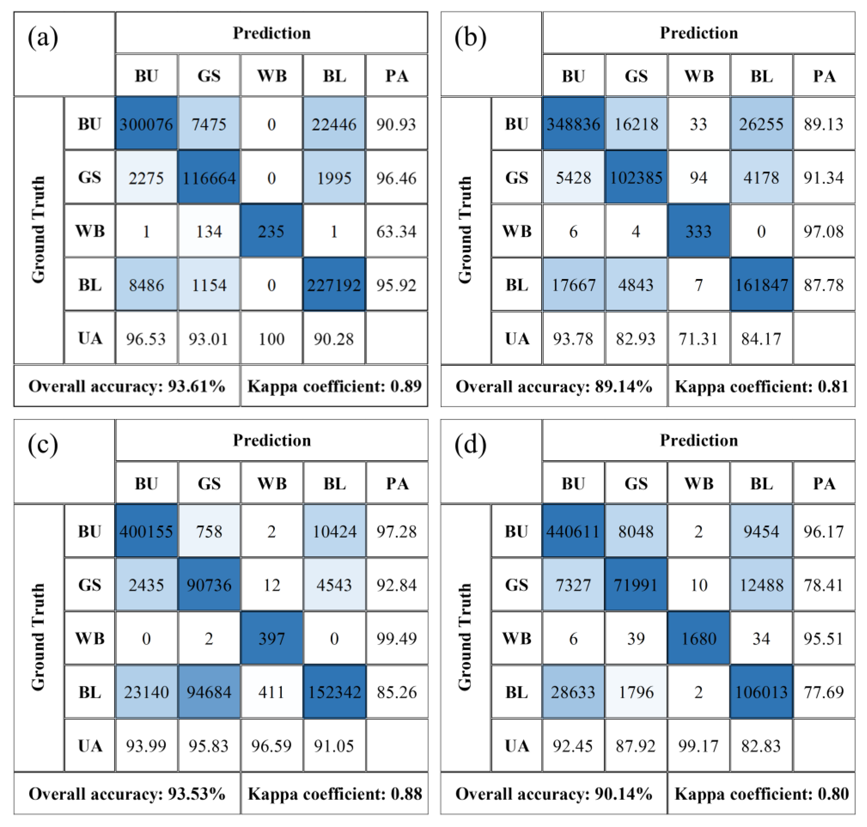
3.2. Land Cover/Land Use (LULC) Mapping

Optical surface reflectance images from both Landsat-5 and Landsat-8 satellites were employed to generate four class LULC maps with 30 m spatial resolution from 1989 to 2019. The produced LULC maps were used to investigate the urbanization trend during the last three decades and also to examine their relationship with the spatio-temporal patterns of SUHI and UTFVI maps for the years 1989, 1999, 2009, and 2019. The Support Vector Machine (SVM) classifier with the Radial Basis Function (RBF) kernel implemented within GEE was utilized to produce LULC maps. SVM is a non-parametric classification algorithm, which is based on fitting optimal separating hyperplanes between different classes by focusing on the training samples that lie at the edge of the distribution of the classes in the features space, called support vectors [59]. It is worth noting that the RBF kernel was used since it provides accurate LULC maps [60], and its necessary tuning parameters were determined based on several trial and error attempts to achieve satisfactory classification results. The generated LULC maps include four classes, namely Water Body (WB, including artificial lakes), Green Space (GS, including urban parks, urban forests, trees, croplands, and grasslands), Bare Land (BL, including unused lands with soil cover), and Built-Up (BU, including human residents, industrial sites, and urban infrastructure). The required reference samples to support the supervised classification tasks were collected by precise visual interpretation of each image, and then they were randomly split into two halves of training and test samples [61]. On average, 248 polygons with an area of about 4.7 km2, including four LULC classes, were collected for each period, and Table A4 provides the number of polygons and area of each land cover for the years 1989, 1999, 2009, and 2019.

3.3. Surface Urban Heat Island (SUHI) Mapping

Generally, SUHI mapping methods are categorized into three groups, namely (1) using LST as a proxy of SUHI, (2) LST differences between urban and the surroundings [13,62] (i.e., reference areas), and (3) statistical methods [20]. The first approach uses LST values to investigate the SUHI variability since the SUHI manifests itself in hotspot forms or high LST values in comparison to the surrounding environment [63]. The main limitation of these approaches is that they avoid the measurement of SUHI intensities and make SUHI comparisons more challenging [20]. In the second category, the LST differences between urban areas and mean LST values of reference areas (e.g., rural, suburban, water, and vegetation) are employed to map the SUHI [38,64]. Although these methods are simple to implement and provide SUHI intensities, they commonly suffer from uncertainties associated with urban and reference areas delineation [65]. The third category utilized statistical algorithms, such as Gaussian Surface Modeling (GSM) and linear regression functions, to generate SUHI maps [66,67]. These approaches are not affected by the biases caused by reference area selection and, thus, facilitate the SUHI comparisons [20].
In this study, the planar fitting and GSM were implemented to map the SUHI areas of Tehran. The GSM model enables a better understanding of the SUHI patterns as it provides the magnitude, spatial extent, and central location of the SUHI. Furthermore, this method allows quantitative comparisons of SUHI maps over timescales for a single city [68]. The GSM was first developed by [69], and then was employed in other studies to delineate SUHI intensity and its spatial extents. A stable workflow to implement the GSM model for SUHI mapping is thoroughly described in [70]; however, brief step-wise explanations are provided in the following. For this task, the first step is to compute the SUHI map based on Equation (4). To this end, the urban areas (BU pixels from the LULC maps) were temporarily masked from the LST images ( T ( x , y ) ; x and y are the pixel coordinates), and then a planar surface was fitted to the existing non-urban LST values to determine T 0 , a 1 , and a 2 . This part attempts to model the spatial pattern of LST in the study area with the assumption of no BU areas. The next step is to subtract the fitted surface from the actual LST with all pixels to extract the SUHI patterns (Equation (4)). Afterward, the GSM, as shown in Equation (5), is fitted to the derived SUHI images using the least-square method. These approaches provide the SUHI characteristics, including SUHI magnitude ( a 0 ), the central location of the primary heat island ( x 0 and y 0 ), its orientation ( φ ), and its spatial extent ( a x and a y ). Furthermore, as an automatic workflow, it eliminated the uncertainties associated with reference area selection [20].
T ( x . y ) = T 0 +   a 1 x + a 2 y +   SUHI ( x . y )
SUHI   ( x , y ) = a 0 * exp [ ( ( x x 0   ) cos φ + ( y y 0 ) sin φ ) 2 0.5 a x 2 ( ( y y 0   ) cos φ ( x x 0 ) sin φ ) 2 0.5 a y 2 ]

3.4. Urban Thermal Filed Variance Index (UTFVI) Mapping

UTFVI, which is calculated based on Equation (6) [71], is an extensively used indicator that describes the environmental condition and quality of urban health through the measure of thermal comfort presence in the environment [25]. Although there are different indices for the evaluation of thermal comfort, they are not applicable in some regions due to the lack of data [72,73,74]. UTFVI notably causes adverse impacts on different socio-economic and environmental issues, including humidity, air quality, indirect economic loss, reduced living comfort, and increased mortality rate [75]. Accordingly, the examination of the UTFVI patterns is attracting more interest in the scientific community since it could provide beneficial information of thermal comfort status, ensuring sustainable development [25]. The calculated UTFVI values were then classified into six classes (see Table 2) for better visualization and to provide explicit environmental condition patterns throughout the city [23].
UTFVI = LST   LST mean LST   mean

4. Results

4.1. Decadal LULC, SUHI, and UTFVI

Figure 3 shows the generated LULC, SUHI, and UTFVI maps over Tehran from 1989 to 2019.
Figure 3a–d illustrates that the city has undergone a substantial LULC change, mainly in terms of urban expansion and the conversion of natural land covers into urban impervious surfaces and BU. In particular, the produced LULC maps, with overall accuracies that varied between 89.14% and 93.61% (see Figure A1), indicate that the BU areas covered 329.49 km2, 387.24 km2, 446.93 km2, and 505.17 km2 of the city in 1989, 1999, 2009, and 2019, respectively. This specifies an approximately 53.33% growth in BU areas over the last three decades. Additionally, the time-series LULC maps generated from 25 Landsat-5 and Landsat-8 images between 1989 and 2019 revealed a gradual upward trend of urbanization with a rate of 5.86 (±2.42) km2 per year in Tehran. According to Figure 3a–d, considerable urban expansions occurred in the western and northern parts of the city due to the construction and development of residential, industrial, and commercial infrastructures. For instance, in 1989, most of the western parts of Tehran were covered by BL and GS, constantly changing to BU by 2019. Moreover, a notable part of GS areas in 1989, especially in the northern parts, were lost and superseded by BU.
Likewise, Figure 3e–h presents the SUHI maps of Tehran between 1989 and 2019. As is clear, the spatial patterns of SUHIs have changed over the past three decades. Visually, the regions in which the SUHI intensities were increased are mostly demarcated in locations where BU areas were developed or BL areas exist. For example, the northern part of the city experienced SUHI intensification that is mainly associated with the drastic reduction of GS areas (see Figure 3a–d), which had eliminated the cooling effect of this land cover. Similarly, the western regions, which have been the center of urban development for the past decades, encountered a significant increase in SUHI intensity. Considering LULC maps (Figure 3a–d), the SUHI intensifications could be partly identified as the consequences of GS loss across Tehran. In addition to SUHI intensity changes over the regions associated with LULC transitions, the city center, which was almost covered by BU in the study period, also experienced a moderate aggravation of this phenomenon. Despite spatial changes of SUHI intensities throughout Tehran, further statistical analysis revealed that the average SUHI intensity in Tehran increased from 2.05 °C to 4.07 °C from 1989 to 2019. This also confirms the necessity of devoting more research studies to examine the SUHI patterns and intensities for further adaption.
The UTFVI maps were also derived from LST images and then were classified into six classes (see Table 2) for better visualization and to provide an explicit spatio-temporal overview of the environmental condition and thermal comfort throughout Tehran (Figure 3i–l). Generally, major BU areas were distributed over two extreme categories of EC and WTC, while small BU patches were demarcated in GC and NC. As in the SUHI maps and urbanization patterns, the western part of Tehran had a higher rate of UTFVI alterations, in which the WTC has spatially expanded except for small patches, including the Chitgar Lake and the surrounding areas. The center and south of the city have also experienced thermal comfort degradation since the WTC patches have enlarged. UTFVI maps of 1989-2009 illustrate that over 55.45% of Tehran was identified as EC, while in 2019, 52.35% and 37.11% were classified as WTC and EC, respectively. The results manifest a 16.37% and 18.34% increase and decrease in the areas of WTC and EC in 2019, respectively, compared to the same classes in 2009.

4.1.1. Relationship between SUHI and LULC

For a more profound comparison between SUHI variations and LULC changes, the SUHI maps were classified into five categories, provided in Table 3.
The classified SUHI maps, along with the corresponding pie charts showing the share of each SUHI class, are presented in Figure 4. It is evident that over the past three decades, the majority (i.e., over 70%) of the city was classified as Medium SUHI. Furthermore, the area of Very Low SUHI had moderate spatial changes and declined by about 2.26% from 1989 to 2019, which was mainly focused on the northern part of the study area. This may be mainly linked to the loss of vegetation covers (i.e., GS) and their replacement with urban impervious surfaces (i.e., BU). The area of Low SUHI increased by about 3.16% over the last three decades, of which further investigations revealed that 60.45% of this class was transited from the Very Low SUHI. Despite the variations of spatial distribution, the High SUHI maintained nearly 9% of Tehran’s area over the study period. Moreover, Very High areas, except for some small patches, were mainly distributed and expanded in the western parts of Tehran, which was also in agreement with impervious surface developments. The Very High area increased by about 3.44% from 1989 to 2019 and reached 10.05% of the entire study area.
Additionally, the distribution of each LULC class at different SUHI categories for 1989, 1999, 2009, and 2019 was extracted by combining the LULC and classified SUHI maps. According to the results (Figure 5), except for the WB, the majority area of other LULC classes had Medium SUHI. The results suggest that the SUHI intensity (i.e., SUHI category) has increased over the BL and BU areas over the last three decades while remaining relatively the same for the other two LULC classes. Moreover, the area of BU with High and Very High SUHI intensities slightly increased from 1989 to 2019, which indicates the necessity for precise monitoring of the SUHI phenomenon, especially in these regions, to adopt mitigation strategies. Likewise, one can see a notable increase in the area of BL with High and Very High SUHI intensities reaching nearly 47.53% in total over the last three decades, which could also cause environmental issues for their proximities. The WB areas mostly included Very Low SUHI that was already expected based on the cooling effect characteristics of this land cover, except for a moderate fluctuation in 1999 that could be linked to the misclassification errors of the LULC maps. Although the area of Very High and High SUHI classes over the GS areas remained the same over time, the total area with Very Low and Low SUHI intensities declined by about 15.49% in 2019, compared to their corresponding utmost values (i.e., 39.12%) in 1999. In addition to the GS loss throughout the city, the thinning of GS cover can also be understood as another reason for this decline due to the weakening of cooling efficiency [76].
To further appraise the impact of GS loss as a great source of SUHI mitigation [8,35], the decadal transition of GS to other LULC classes and the related SUHI intensity changes were investigated (see Table 4). Considering Table 4, the most significant transition of GS to other LULC classes, with a total area of 51.32 km2, occurred from 1999 to 2009. This considerable LULC change has also been accompanied by an increment in the SUHI intensity. In particular, the conversion of 20.61% of GS to BL from 1999 to 2009 resulted in a 2.16 °C rise in SUHI intensity in the corresponding locations. Likewise, the replacement of 18.61% of GS with BU areas led to a 1.24 °C growth in the SUHI intensity. After LULC changes between 1999 and 2009, the most extensive variation in GS occurred from 1989 to 1999 with a 40.03 km2 loss of GS, which resulted in an average SUHI intensification of about 1.02 °C in the transition zones. In total, regarding the GS conversion to other LULC classes from 1989 to 2019, approximately 85.76 km2 of GS disappeared, by which the SUHI intensity experienced an average rise of about 2.84 °C in the changed areas, leading to SUHI intensification throughout the city.

4.1.2. Relationship between UTFVI and LULC

In order to examine the status of the LULC classes in terms of environmental condition and thermal comfort, the relative percentage of each class for the two UTFVI classes of EC and WTC for 1989, 1999, 2009, and 2019 were extracted (Figure 6). It is worth noting that only two extreme UTFVI classes were considered since these two classes cover nearly 90% of the study area. In general, during the last three decades, all LULC classes had downward trends in EC and upward trends in WTC. According to the results, BL areas were dominantly demarcated in WTC in all time intervals. The BL areas had the most environmental change in the last three decades. In particular, the area of BL with EC declined from 28.60% in 1989 to about 10% in 2019, and meanwhile, the BL area with WTC grew by about 22.53%, reaching 84.95% in 2019. In contrast, WB and GS areas were located mostly in EC; however, the GS experienced a more severe degradation (i.e., a downward trend in EC and an upward trend in WTC) in environmental conditions, which could probably be linked to the loss and thinning of GS cover. More importantly, Figure 6a shows that in 1989, over 61.35% of BU areas were located in EC, while in 2019, this percentage considerably decreased by about 19.01%, reaching 42.34%. Likewise, an unfavorable upward trend can be seen in Figure 6b, in which nearly 45.31% of the BU areas were demarcated in WTC. Consequently, the results confirmed that from 1989 to 2019, the BU, which is the permanent habitat of people, experienced significant thermal comfort decay. These adverse environmental conditions in BU areas can be associated with considerable urban expansions in unsuitable western parts of the city, which have also been classified as WTC in the earlier year of this study.

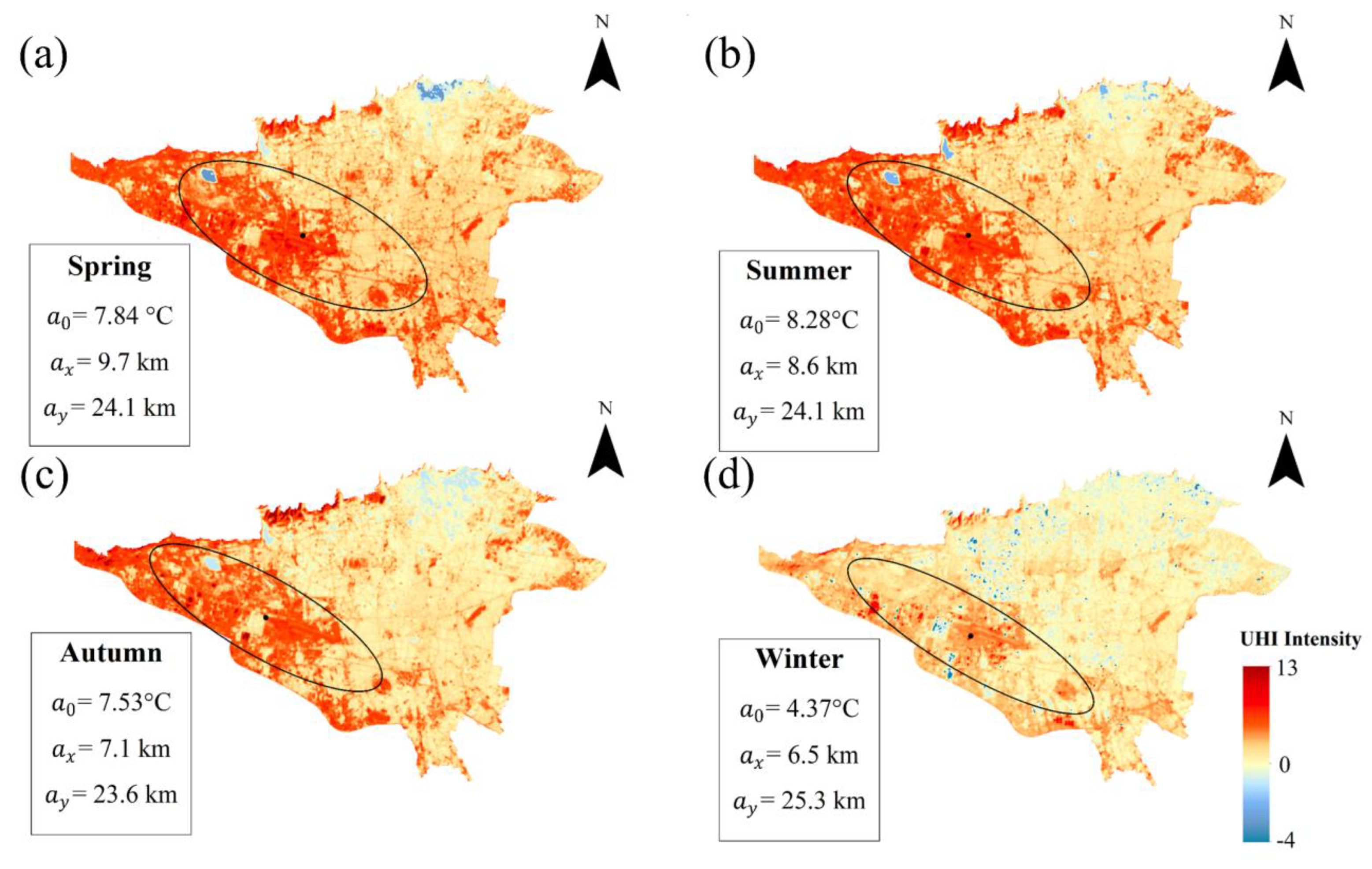
4.2. Intra-Annual Variation of SUHI

Seasonal variations of SUHI were also examined in the most recent year (i.e., 2019) of the study period to obtain an overview of the current spatio-temporal SUHI status. This analysis can provide practical information for future planning to promote a sustainable city. In this regard, the pattern and descriptive characteristics of the GSM are represented in Figure 7. Figure 7a–d illustrates the center and spatial footprint of primary SUHI, using an ellipse with an orientation of φ and major and minor axes that are equal to a x and a y . As is clear, the SUHI throughout Tehran generally had higher intensity in summer and spring. It is evident that summer had the highest SUHI magnitude of 8.28 °C with the greatest SUHI footprint, while the winter had the lowest SUHI magnitude of 4.37 °C. The GSM results implied that almost the western and southwestern regions of the city, where the center of SUHI was located in all seasons, had the highest rate of this phenomenon. This could be related to the development and concentration of industrial infrastructure and urban expansions in these regions. It is worth mentioning that there were other parts of the city with SUHI hotspots; however, the GSM model attempted to find and fit the greatest SUHI hotspot in the study area. Furthermore, the visual inspection of the results revealed that despite the concentrated patches with high SUHI intensity, the road networks with impervious surfaces, especially in the center of the city, included high SUHI intensity. This may be rooted in the fact that these roads in the city center mostly suffer from high traffic and the related heat from the combustion of fossil fuels.
As already discussed in detail in Section 4.1., the study area has undergone a significant LULC change in the past three decades. Here, the seasonal variations of SUHI intensities in different seasons between 1989 and 2019 were also explored. According to Table 5, the average SUHI intensities of all LULC classes in each season have modestly increased from 1989 to 2019. For instance, the BL average SUHI in summer 1989 increased by about 2.35 °C and reached 7.39 °C in summer 2019. Likewise, the average SUHI intensities over BU in spring from 1989 to 2019 rose from 2.86 °C to 4.44 °C. In total, the results revealed that the rise of the SUHI intensity itself through time and the LULC changes, in addition to causing a higher amount of LULC classes to experience higher SUHI intensities, have increased the average SUHI intensity throughout the city and decreased the thermal comfort and quality of the city.

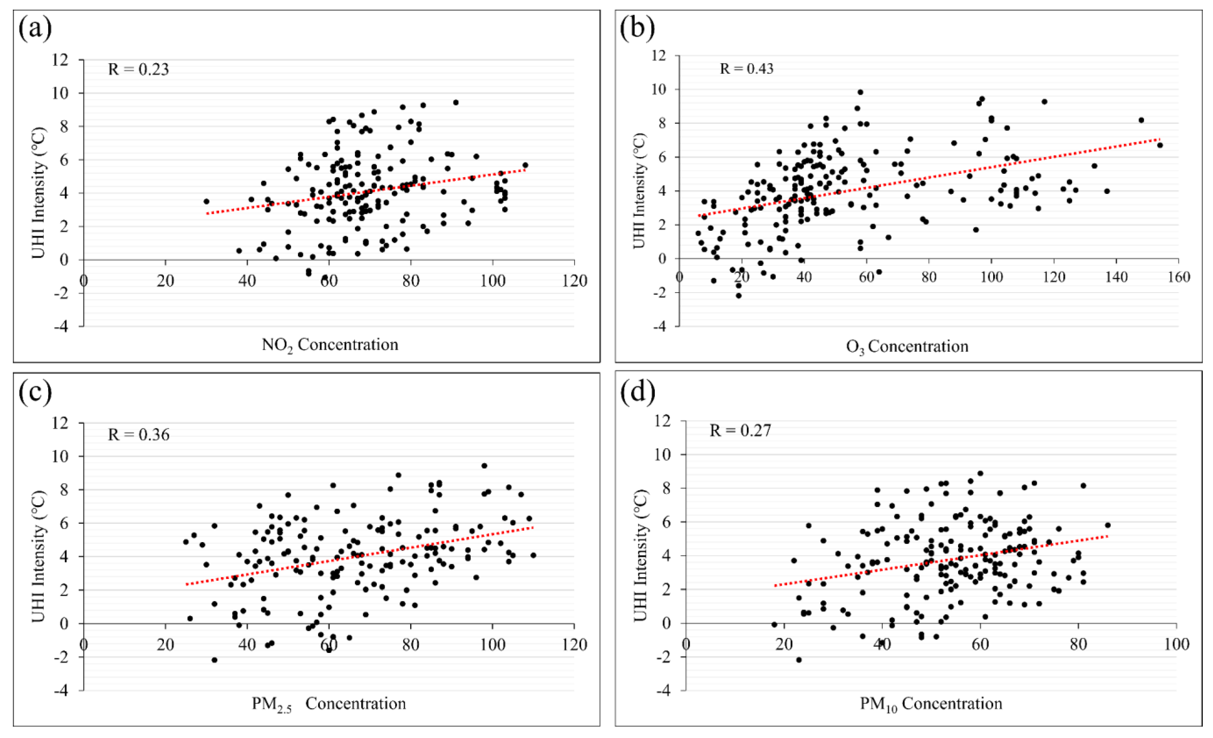
4.3. Relationship between SUHI and AP

Air pollution is an influential factor on LST and consequently on SUHI intensity [77]. However, contradicting reports on the relationship between air pollutants and SUHI intensity in different regions [45,46,47,48] necessitate local studies to appraise their relationship in Tehran. In particular, these types of investigations should be examined through case-specific studies to ensure the selection of efficient strategies due to the complex and different characteristics of urban areas [46]. Accordingly, the results can assist in adopting more efficient strategies for the mitigation of these two adverse environmental phenomena [78]. Here, five different air pollutants, including NO2, O3, PM2.5, and PM10, were considered to discover their relationships with SUHI intensity. Figure 8 illustrates the generally positive relationships between daily pollutants concentration and SUHI intensity in 2019. To estimate the strength of bivariate associations between SUHI and air pollutants, the Correlation Coefficient (CC) values were calculated. Considering the annual investigations, O3 and NO2 had the highest and lowest CC values of 0.43 and 0.23, respectively. Furthermore, the CC values were also computed in seasonal time scales. According to the results, the highest CC values for O3 (0.64) and PM10 (0.60) were observed in autumn, while NO2 (0.43) had the highest CC value in spring. Additionally, PM2.5 was the only pollutant that had almost steady behavior in all seasons, with an average CC value of 0.48. The discrepancies in seasonal CC values could be linked to other climate and meteorological factors such as wind speed, boundary layer structure, weather conditions, solar radiation, temperature inversion, and humidity [48,79]. The results indicate that these two environmental issues had a positive relationship, and an increase in one can strengthen the other and, thus, should be properly monitored since they are threats to human life and degrade the quality of life in metropolitan areas [80,81].

5. Discussion

Due to socio-economic and political conditions, Tehran has experienced a high rate of population rise in recent decades, which has led to Tehran being named one of the cities with the highest annual growth in Asia [34]. These demographic changes were accompanied by an increase in demands for urban facilities and resulted in a massive conversion of natural land covers to urban impervious surfaces [28]. This study illustrated that from 1989 to 2019, the dramatic urban expansion was accompanied by a considerable increase in the agglomeration of BU areas during each decadal interval (Figure 3). The sharp rise in BU constructions, especially in the western part of Tehran, has altered the thermodynamic properties of the surface and increased LST. The decadal examination of SUHI patterns throughout the city indicated the deterioration of thermal conditions in the study area. One of the main consequences of urbanization that emerged with the land cover transition was creating and intensifying SUHIs [82]. Some of the factors that have contributed to the aggregated growth of SUHI intensity include population growth, an increase in BU areas, the expansion of industrial activities, GS cover reduction, and changes in the intensity of solar radiation [52,83]. Different studies have focused on the appraisal of LULC transitions on increasing LST and SUHI. Furthermore, researchers have reported a negative relationship between GS cover and SUHI intensity and its significant role in mitigating the SUHI intensity [84]. Considering Tehran, the northern part of the city had the most considerable cooling effect associated with dense GS cover. However, over the last three decades, notable GS areas disappeared, and as a result, the SUHI intensity increased. Despite the GS loss, the thinning of GS density due to land cover changes also weakened the cooling efficiency of the remnant GS areas [76]. Taking the current structure of Tehran and the urban morphology, it may be practically infeasible and resource-intensive to create new large GS (i.e., parks and forests) areas within the hotspot zones of SUHI and, thus, it would be more cost-effective to establish new policies to encourage the use of green and cool roofs to mitigate the SUHI intensities [85], which can be followed up in future studies. Furthermore, utilizing high-albedo materials for roofs, pavements, and roads can also help mitigate SUHI and cool the city [86]. Additionally, the decadal analyses of the thermal comfort of the city through the UTFVI index demonstrated that the environmental condition of the city experienced a notable decay. More importantly, currently, 45.31% of BU exists in WTC zones that can potentially threaten human health. Despite other natural and climate-related factors that contributed to the environmental decay of Tehran, the construction of BU areas in locations with WTC in earlier decades has caused the unsuitable environmental condition of the majority of BU areas in Tehran. Therefore, it could be stated that the current status of the environmental condition of Tehran should be considered before any possible urban expansion to avoid further degradations of thermal comfort in BU areas.
Tehran is suffering from high-density air pollution [44]. Population growth, fossil fuel consumption, and the reduction of local winds due to vast vertical urban expansion have played essential roles in increasing the air pollutant concentration in Tehran. Additionally, urban growth, the conversion of natural land cover to buildings and human residents, and climate change have all enhanced the UHI intensity throughout the city. The preliminary analysis in this study reveals the positive interaction between SUHI and AP, which is also in accordance with similar studies in other areas [77,87,88]. In fact, high pollutant concentrations can trap more earth-emitted infrared radiation and heat in the urban environment, thus increasing the temperature [89]. Consequently, it is possible to incorporate suitable strategies to simultaneously reduce the SUHI intensity and AP concentration [90]. For instance, urban greening (i.e., increasing the vegetation cover through the city, especially in hotspot zones) is known to be an effective approach to mitigate the SUHI intensity. In this case, an efficient strategy would be choosing appropriate plant/tree species that have higher pollutant tolerance [90]. For example, Currie and Bass [91] found that extending green roofs by grass or shrubs can significantly mitigate AP, and it is well known that green roofs were stated to be one of the suitable approaches for UHI mitigation. Likewise, a model estimated by Yang et al. [92] indicated that increasing green roofs by about 20 ha can remove nearly 1700 kg of air pollutions during one year in Chicago. Furthermore, alterations in the urban microclimate can influence pollutant dispersion [90]. In particular, SUHI-related warm temperatures in urban areas affect the atmospheric turbulence and increase the boundary layer’s height, leading to higher air pollution concentration [7,93]. Accordingly, SUHI mitigation will remove the effect that excessive warm temperatures have on atmospheric turbulence. For instance, Epstein et al. [94] reported that a decrease of about 0.35 k in the UHI intensity can decrease the urban boundary layer height by about 60%, thus boosting the dispersion of aerosol particles inside a deeper boundary layer, decreasing the aerosol concentration.
In this paper, Landsat-5 and Landsat-8 satellite images were collected from GEE. This geospatial cloud platform helps to reduce the dedicated time and effort for repetitive tasks, including pre-processing, image acquisition, and calibrating, of time-series satellite data [95]. Accordingly, it is recommended to exploit the considerable potential of GEE for long-term urban studies, especially for LULC, SUHI, and UTFVI mapping and monitoring.

6. Conclusions

Time-series Landsat-5 and Landsat-8 satellite images were employed to study the spatio-temporal variations of LULC, SUHI, and UTFVI throughout Tehran. The main findings of this study include the following:
The generated LULC maps indicated that the simultaneous loss of GS areas along with the expansion of BU areas have contributed toward SUHI intensification by an average of 2.02 °C over the last three decades.
The seasonal SUHI investigations revealed that the summer had the highest SUHI magnitude and footprint in Tehran.
The UTFVI analysis revealed that the thermal comfort condition of Tehran has been significantly degraded since 52.35% of the city was identified as WTC, which was increased by about 16.37% compared with 2009.
Notable thermal comfort degradation, especially in BU areas, was also associated with arbitrary urban expansion in the western part of Tehran since these regions were also classified as WTC even in earlier years when no BU existed.
The preliminary results of comparing SUHI intensities and AP (i.e., NO2, O3, PM2.5, and PM10) concentrations indicated positive CC values between these two environmental phenomena in Tehran, which could be considered to adopt two-way mitigation strategies.
Policymakers and urban managers can employ the results of this study to avoid further environmental degradation in Tehran and assist with movement toward a sustainable city. In this regard, urban greening (i.e., by expanding urban parks, forests, and green roofs) can be considered to improve the environmental condition of Tehran. Determining and allocating pollution-tolerant plant species with reasonable cooling effects can be considered as the next step to enhance the quality of life in Tehran.

Author Contributions

Conceptualization, F.N. and A.G.; methodology, F.N. and A.G.; software, F.N.; validation, F.N.; formal analysis, F.N.; investigation, F.N., A.M., A.G. and S.J.; resources, F.N.; data curation, F.N.; writing—original draft preparation, F.N. and A.G.; writing—review and editing, F.N., A.M., A.G. and S.J.; visualization, F.N.; supervision, A.M. and S.J. All authors have read and agreed to the published version of the manuscript.

Funding

This research received no external funding.

Institutional Review Board Statement

Not applicable.

Informed Consent Statement

Not applicable.

Data Availability Statement

Landsat satellite images and air pollutant concentration values are publicly available from (https://developers.google.com/earth-engine/datasets/catalog/landsat accessed on 10 January 2020) and (https://air.tehran.ir accessed on 10 January 2020), respectively.

Acknowledgments

The authors would like to thank the United States Geological Survey (USGS) and Tehran Air Quality Control Company to freely provide Landsat Archive satellite data and air pollutant concentration values, respectively. Additionally, the authors thank the three anonymous reviewers for their constructive comments.

Conflicts of Interest

The authors declare no conflict of interest.

Appendix A

Table A1. The nomenclature of all abbreviations used in this paper.
AbbreviationsDefinitionsAbbreviationsDefinitions
ANNArtificial Neural NetworksNCNormal Condition
ASTERThermal Emission and Reflection RadiometerNDVINormalized Difference Vegetation Index
BCBad ConditionOLIOperational Land Imager
BLBare LandPMParticulate Matter
BUBuilt-UpRBFRadial Basis Function
CA-MCellular Automata-MarkovSDStandard Deviation
CCCorrelation CoefficientSUHISurface Urban Heat Island
CF MaskC Function of MaskSVMSupport Vector Machine
ECExcellent ConditionTIRThermal Infrared
GCGood ConditionTIRSThermal Infrared Sensor
GEEGoogle Earth EngineTMThematic Mapper
GSGreen SpaceUHIUrban Heat Island
GSMGaussian Surface ModelUSGSUnited States Geological Survey
LaSRCLand Surface Reflectance CodeUTFVIUrban Thermal Field Variance Index
LEDAPSLandsat Ecosystem Distribution Adaptive Processing SystemWBWater Body
LSTLand Surface TemperatureWCWorse Condition
LULCLand Use/Land CoverWTCWorst Condition
NASANational Aeronautics and Space Administration
Table A2. Brief specification of satellite images used for LUCL, UHI, UTFVI, and NDVI mapping over the study area.
ResultSatelliteBandsSpatial Resolution (m)Number of ImagesDates
LULCLandsat-51, 2, 3, 4, 5, and 7301810/06/1989, 13/06/1990, 16/06/1991, 18/06/1992, 25/09/1993, 12/09/1994, 11/06/1995, 17/09/1996, 13/04/1997, 05/07/1998, 24/07/1999, 12/09/2000, 29/07/2001, 30/06/2002, 30/06/2008, 13/03/2009, 04/06/2010, 09/07/2011
Landsat-82, 3, 4, 5, 6, and 730716/09/2013, 18/08/2014, 05/08/2015, 07/08/2016, 25/07/2017, 26/06/2018, 31/07/2019
UHI, UTFVI, and NDVILandsat-5630/120 m3201/01/1989, 06/03/1989, 25/05/1989, 10/06/1989, 26/06/1989, 29/08/1989, 14/09/1989, 30/09/1989, 16/10/1989, 13/01/1999, 18/03/1999, 19/04/1999, 05/05/1999, 21/05/1999, 06/06/1999, 08/07/1999, 24/07/1999, 09/08/1999, 10/09/1999, 12/10/1999, 13/11/1999, 13/03/2009, 01/06/2009, 17/06/2009, 03/07/2009, 19/07/2009, 04/08/2009, 05/09/2009, 21/09/2009, 07/10/2009, 08/11/2009, 24/11/2009
Landsat-81030/100 m1504/01/2019, 05/02/2019, 21/02/2019, 10/04/2019, 12/05/2019, 28/05/2019, 13/06/2019, 29/06/2019, 15/07/2019, 31/07/2019, 16/08/2019, 01/09/2019, 17/09/2019, 03/10/2019, 19/10/2019
The NDVI images were calculated to apply emissivity correction of LST images. In total, 47 Landsat-5 and 21 Landsat-8 scenes were considered. There are several common image dates between the two above categories.
Table A3. ImageCollection IDs of Landsat-5 and Landsat-8 datasets of this study.
  • LANDSAT/LT05/C01/T1_SR/LT05_164035_19890101
  • LANDSAT/LT05/C01/T1_SR/LT05_164035_19890306
  • LANDSAT/LT05/C01/T1_SR/LT05_164035_19890525
  • LANDSAT/LT05/C01/T1_SR/LT05_164035_19890610
  • LANDSAT/LT05/C01/T1_SR/LT05_164035_19890626
  • LANDSAT/LT05/C01/T1_SR/LT05_164035_19890829
  • LANDSAT/LT05/C01/T1_SR/LT05_164035_19890914
  • LANDSAT/LT05/C01/T1_SR/LT05_164035_19890930
  • LANDSAT/LT05/C01/T1_SR/LT05_164035_19891016
  • LANDSAT/LT05/C01/T1_SR/LT05_164035_19900613
  • LANDSAT/LT05/C01/T1_SR/LT05_164035_19910616
  • LANDSAT/LT05/C01/T1_SR/LT05_164035_19920618
  • LANDSAT/LT05/C01/T1_SR/LT05_164035_19930925
  • LANDSAT/LT05/C01/T1_SR/LT05_164035_19940912
  • LANDSAT/LT05/C01/T1_SR/LT05_164035_19950611
  • LANDSAT/LT05/C01/T1_SR/LT05_164035_19960917
  • LANDSAT/LT05/C01/T1_SR/LT05_164035_19970413
  • LANDSAT/LT05/C01/T1_SR/LT05_164035_19980705
  • LANDSAT/LT05/C01/T1_SR/LT05_164035_19990113
  • LANDSAT/LT05/C01/T1_SR/LT05_164035_19990318
  • LANDSAT/LT05/C01/T1_SR/LT05_164035_19990419
  • LANDSAT/LT05/C01/T1_SR/LT05_164035_19990505
  • LANDSAT/LT05/C01/T1_SR/LT05_164035_19990521
  • LANDSAT/LT05/C01/T1_SR/LT05_164035_19990606
  • LANDSAT/LT05/C01/T1_SR/LT05_164035_19990708
  • LANDSAT/LT05/C01/T1_SR/LT05_164035_19990724
  • LANDSAT/LT05/C01/T1_SR/LT05_164035_19990809
  • LANDSAT/LT05/C01/T1_SR/LT05_164035_19990910
  • LANDSAT/LT05/C01/T1_SR/LT05_164035_19991012
  • LANDSAT/LT05/C01/T1_SR/LT05_164035_19991113
  • LANDSAT/LT05/C01/T1_SR/LT05_164035_20000912
  • LANDSAT/LT05/C01/T1_SR/LT05_164035_20010729
  • LANDSAT/LT05/C01/T1_SR/LT05_164035_20020630
  • LANDSAT/LT05/C01/T1_SR/LT05_164035_20080630
35.
LANDSAT/LT05/C01/T1_SR/LT05_164035_20090313
36.
LANDSAT/LT05/C01/T1_SR/LT05_164035_20090601
37.
LANDSAT/LT05/C01/T1_SR/LT05_164035_20090617
38.
LANDSAT/LT05/C01/T1_SR/LT05_164035_20090703
39.
LANDSAT/LT05/C01/T1_SR/LT05_164035_20090719
40.
LANDSAT/LT05/C01/T1_SR/LT05_164035_20090804
41.
LANDSAT/LT05/C01/T1_SR/LT05_164035_20090905
42.
LANDSAT/LT05/C01/T1_SR/LT05_164035_20090921
43.
LANDSAT/LT05/C01/T1_SR/LT05_164035_20091007
44.
LANDSAT/LT05/C01/T1_SR/LT05_164035_20091108
45.
LANDSAT/LT05/C01/T1_SR/LT05_164035_20091124
46.
LANDSAT/LT05/C01/T1_SR/LT05_164035_20100604
47.
LANDSAT/LT05/C01/T1_SR/LT05_164035_20110709
48.
LANDSAT/LC08/C01/T1_SR/LC08_164035_20130916
49.
LANDSAT/LC08/C01/T1_SR/LC08_164035_20140818
50.
LANDSAT/LC08/C01/T1_SR/LC08_164035_20150805
51.
LANDSAT/LC08/C01/T1_SR/LC08_164035_20160807
52.
LANDSAT/LC08/C01/T1_SR/LC08_164035_20170725
53.
LANDSAT/LC08/C01/T1_SR/LC08_164035_20180626
54.
LANDSAT/LC08/C01/T1_SR/LC08_164035_20190104
55.
LANDSAT/LC08/C01/T1_SR/LC08_164035_20190205
56.
LANDSAT/LC08/C01/T1_SR/LC08_164035_20190221
57.
LANDSAT/LC08/C01/T1_SR/LC08_164035_20190410
58.
LANDSAT/LC08/C01/T1_SR/LC08_164035_20190512
59.
LANDSAT/LC08/C01/T1_SR/LC08_164035_20190528
60.
LANDSAT/LC08/C01/T1_SR/LC08_164035_20190613
61.
LANDSAT/LC08/C01/T1_SR/LC08_164035_20190629
62.
LANDSAT/LC08/C01/T1_SR/LC08_164035_20190715
63.
LANDSAT/LC08/C01/T1_SR/LC08_164035_20190731
64.
LANDSAT/LC08/C01/T1_SR/LC08_164035_20190816
65.
LANDSAT/LC08/C01/T1_SR/LC08_164035_20190901
66.
LANDSAT/LC08/C01/T1_SR/LC08_164035_20190917
67.
LANDSAT/LC08/C01/T1_SR/LC08_164035_20191003
68.
LANDSAT/LC08/C01/T1_SR/LC08_164035_20191019
Table A4. Number and area of reference samples were collected using satellite images to support the supervised classification task for LULC mapping.
IDClass1989199920092019
PolygonsArea (ha)PolygonsArea (ha)PolygonsArea (ha)PolygonsArea (ha)
1Built-Up6484.016790.667194.3877105.62
2Bare Land83199.8584208.1981193.7880189.38
3Green Space78169.5983193.0982180.3076163.77
4Water Body147.38147.38147.382515.89
Total239460.83248499.33247475.84258474.66
Figure A1. Confusion matrix of (a) 1989, (b) 1999, (c) 2009, and (d) 2019 Land Use/Land Cover (LULC) maps of Tehran.
Remotesensing 13 04469 g0a1

References

  1. Ye, C.; Wang, M.; Li, J. Derivation of the characteristics of the Surface Urban Heat Island in the Greater Toronto area using thermal infrared remote sensing. Remote Sens. Lett. 2017, 8, 637–646. [Google Scholar] [CrossRef]
  2. Li, X.; Zhou, W. Spatial patterns and driving factors of surface urban heat island intensity: A comparative study for two agriculture-dominated regions in China and the USA. Sustain. Cities Soc. 2019, 48, 101518. [Google Scholar] [CrossRef]
  3. Gaur, A.; Eichenbaum, M.K.; Simonovic, S.P. Analysis and modelling of surface Urban Heat Island in 20 Canadian cities under climate and land-cover change. J. Environ. Manag. 2018, 206, 145–157. [Google Scholar] [CrossRef] [PubMed]
  4. Zipper, S.C.; Schatz, J.; Singh, A.; Kucharik, C.J.; Townsend, P.A.; Loheide, S.P., II. Urban heat island impacts on plant phenology: Intra-urban variability and response to land cover. Environ. Res. Lett. 2016, 11, 54023. [Google Scholar] [CrossRef]
  5. Krause, C.W.; Lockard, B.; Newcomb, T.J.; Kibler, D.; Lohani, V.; Orth, D.J. Predicting influences of urban development on thermal habitat in a warm water stream. JAWRA J. Am. Water Resour. Assoc. 2004, 40, 1645–1658. [Google Scholar] [CrossRef]
  6. Gu, Y.; Li, D. A modeling study of the sensitivity of urban heat islands to precipitation at climate scales. Urban Clim. 2018, 24, 982–993. [Google Scholar] [CrossRef]
  7. Li, H.; Meier, F.; Lee, X.; Chakraborty, T.; Liu, J.; Schaap, M.; Sodoudi, S. Interaction between urban heat island and urban pollution island during summer in Berlin. Sci. Total Environ. 2018, 636, 818–828. [Google Scholar] [CrossRef]
  8. Jacobs, S.J.; Gallant, A.J.E.; Tapper, N.J.; Li, D. Use of cool roofs and vegetation to mitigate urban heat and improve human thermal stress in Melbourne, Australia. J. Appl. Meteorol. Climatol. 2018, 57, 1747–1764. [Google Scholar] [CrossRef]
  9. Santamouris, M.; Cartalis, C.; Synnefa, A.; Kolokotsa, D. On the impact of urban heat island and global warming on the power demand and electricity consumption of buildings—A review. Energy Build. 2015, 98, 119–124. [Google Scholar] [CrossRef]
  10. Swamy, G.; Nagendra, S.M.S.; Schlink, U. Urban heat island (UHI) influence on secondary pollutant formation in a tropical humid environment. J. Air Waste Manag. Assoc. 2017, 67, 1080–1091. [Google Scholar] [CrossRef] [PubMed] [Green Version]
  11. Sarif, M.; Rimal, B.; Stork, N.E. Assessment of Changes in Land Use/Land Cover and Land Surface Temperatures and Their Impact on Surface Urban Heat Island Phenomena in the Kathmandu Valley (1988–2018). ISPRS Int. J. Geo Inf. 2020, 9, 726. [Google Scholar] [CrossRef]
  12. 2018 Revision of World Urbanization Prospects; UN DESA: New York, NY, USA, 2018.
  13. Estoque, R.C.; Murayama, Y. Monitoring surface urban heat island formation in a tropical mountain city using Landsat data (1987–2015). ISPRS J. Photogramm. Remote Sens. 2017, 133, 18–29. [Google Scholar] [CrossRef]
  14. Gui, X.; Wang, L.; Yao, R.; Yu, D.; Li, C.A. Investigating the urbanization process and its impact on vegetation change and urban heat island in Wuhan, China. Environ. Sci. Pollut. Res. 2019, 26, 30808–30825. [Google Scholar] [CrossRef]
  15. Harmay, N.S.M.; Kim, D.; Choi, M. Urban Heat Island associated with Land Use/Land Cover and climate variations in Melbourne, Australia. Sustain. Cities Soc. 2021, 69, 102861. [Google Scholar] [CrossRef]
  16. Dewan, A.; Kiselev, G.; Botje, D.; Mahmud, G.I.; Bhuian, M.H.; Hassan, Q.K. Surface urban heat island intensity in five major cities of Bangladesh: Patterns, drivers and trends. Sustain. Cities Soc. 2021, 71, 102926. [Google Scholar] [CrossRef]
  17. Han, J.; Liu, J.; Liu, L.; Ye, Y. Spatiotemporal Changes in the Urban Heat Island Intensity of Distinct Local Climate Zones: Case Study of Zhongshan District, Dalian, China. Complexity 2020, 2020, 8820338. [Google Scholar] [CrossRef]
  18. Weng, Q.; Lu, D.; Schubring, J. Estimation of land surface temperature–vegetation abundance relationship for urban heat island studies. Remote Sens. Environ. 2004, 89, 467–483. [Google Scholar] [CrossRef]
  19. Firozjaei, M.K.; Kiavarz, M.; Alavipanah, S.K.; Lakes, T.; Qureshi, S. Monitoring and forecasting heat island intensity through multi-temporal image analysis and cellular automata-Markov chain modelling: A case of Babol city, Iran. Ecol. Indic. 2018, 91, 155–170. [Google Scholar] [CrossRef]
  20. Zhou, D.; Xiao, J.; Bonafoni, S.; Berger, C.; Deilami, K.; Zhou, Y.; Frolking, S.; Yao, R.; Qiao, Z.; Sobrino, J.A. Satellite remote sensing of surface urban heat islands: Progress, challenges, and perspectives. Remote Sens. 2019, 11, 48. [Google Scholar] [CrossRef] [Green Version]
  21. Weng, Q.; Firozjaei, M.K.; Sedighi, A.; Kiavarz, M.; Alavipanah, S.K. Statistical analysis of surface urban heat island intensity variations: A case study of Babol city, Iran. GIScience Remote Sens. 2019, 56, 576–604. [Google Scholar] [CrossRef]
  22. Zhao, C.; Jensen, J.L.R.; Weng, Q.; Currit, N.; Weaver, R. Use of Local Climate Zones to investigate surface urban heat islands in Texas. GIScience Remote Sens. 2020, 57, 1083–1101. [Google Scholar] [CrossRef]
  23. Guha, S.; Govil, H.; Dey, A.; Gill, N. Analytical study of land surface temperature with NDVI and NDBI using Landsat 8 OLI and TIRS data in Florence and Naples city, Italy. Eur. J. Remote Sens. 2018, 51, 667–678. [Google Scholar] [CrossRef]
  24. Alfraihat, R.; Mulugeta, G.; Gala, T. Ecological evaluation of urban heat island in Chicago City, USA. J. Atmos. Pollut. 2016, 4, 23–29. [Google Scholar]
  25. Kafy, A.-A.; Rahman, M.S.; Islam, M.; Al Rakib, A.; Islam, M.A.; Khan, M.H.H.; Sikdar, M.S.; Sarker, M.H.S.; Mawa, J.; Sattar, G.S.; et al. Prediction of seasonal urban thermal field variance index using machine learning algorithms in Cumilla, Bangladesh. Sustain. Cities Soc. 2021, 64, 102542. [Google Scholar] [CrossRef]
  26. Singh, P.; Kikon, N.; Verma, P. Impact of land use change and urbanization on urban heat island in Lucknow city, Central India. A remote sensing based estimate. Sustain. Cities Soc. 2017, 32, 100–114. [Google Scholar] [CrossRef]
  27. Bokaie, M.; Zarkesh, M.K.; Arasteh, P.D.; Hosseini, A. Assessment of urban heat island based on the relationship between land surface temperature and land use/land cover in Tehran. Sustain. Cities Soc. 2016, 23, 94–104. [Google Scholar] [CrossRef]
  28. Rousta, I.; Sarif, M.O.; Gupta, R.D.; Olafsson, H.; Ranagalage, M.; Murayama, Y.; Zhang, H.; Mushore, T.D. Spatiotemporal analysis of land use/land cover and its effects on surface urban heat island using Landsat data: A case study of Metropolitan City Tehran (1988–2018). Sustainability 2018, 10, 4433. [Google Scholar] [CrossRef] [Green Version]
  29. Liu, X.; Zhou, Y.; Yue, W.; Li, X.; Liu, Y.; Lu, D. Spatiotemporal patterns of summer urban heat island in Beijing, China using an improved land surface temperature. J. Clean. Prod. 2020, 257, 120529. [Google Scholar] [CrossRef]
  30. Sultana, S.; Satyanarayana, A.N.V. Assessment of urbanisation and urban heat island intensities using landsat imageries during 2000–2018 over a sub-tropical Indian City. Sustain. Cities Soc. 2020, 52, 101846. [Google Scholar] [CrossRef]
  31. Shirani-Bidabadi, N.; Nasrabadi, T.; Faryadi, S.; Larijani, A.; Roodposhti, M.S. Evaluating the spatial distribution and the intensity of urban heat island using remote sensing, case study of Isfahan city in Iran. Sustain. Cities Soc. 2019, 45, 686–692. [Google Scholar] [CrossRef]
  32. De Faria Peres, L.; de Lucena, A.J.; Rotunno Filho, O.C.; de Almeida França, J.R. The urban heat island in Rio de Janeiro, Brazil, in the last 30 years using remote sensing data. Int. J. Appl. Earth Obs. Geoinf. 2018, 64, 104–116. [Google Scholar] [CrossRef]
  33. Nadizadeh Shorabeh, S.; Hamzeh, S.; Zanganeh Shahraki, S.; Firozjaei, M.K.; Jokar Arsanjani, J. Modelling the intensity of surface urban heat island and predicting the emerging patterns: Landsat multi-temporal images and Tehran as case study. Int. J. Remote Sens. 2020, 41, 7400–7426. [Google Scholar] [CrossRef]
  34. Sharifi, A.; Hosseingholizadeh, M. The effect of rapid population growth on urban expansion and destruction of green space in Tehran from 1972 to 2017. J. Indian Soc. Remote Sens. 2019, 47, 1063–1071. [Google Scholar] [CrossRef]
  35. Farhadi, H.; Faizi, M.; Sanaieian, H. Mitigating the urban heat island in a residential area in Tehran: Investigating the role of vegetation, materials, and orientation of buildings. Sustain. Cities Soc. 2019, 46, 101448. [Google Scholar] [CrossRef]
  36. Jahangir, M.S.; Moghim, S. Assessment of the urban heat island in the city of Tehran using reliability methods. Atmos. Res. 2019, 225, 144–156. [Google Scholar] [CrossRef]
  37. Bokaie, M.; Shamsipour, A.; Khatibi, P.; Hosseini, A. Seasonal monitoring of urban heat island using multi-temporal Landsat and MODIS images in Tehran. Int. J. Urban Sci. 2019, 23, 269–285. [Google Scholar] [CrossRef]
  38. Haashemi, S.; Weng, Q.; Darvishi, A.; Alavipanah, S.K. Seasonal variations of the surface urban heat island in a semi-arid city. Remote Sens. 2016, 8, 352. [Google Scholar] [CrossRef] [Green Version]
  39. Sadeghinia, A.; Alijani, B.; Zeaieanfirouzabadi, P. Analysis of Spatial-Temporal Structure of the Urban Heat Island in Tehran through Remote Sensing and Geographical Information System. J. Geogr. Environ. Hazards 2013, 1, 1–17. [Google Scholar]
  40. Hashemi Darebadami, S.; Darvishi Boloorani, A.; AlaviPanah, S.K.; Bayat, R. Investigation of changes in surface urban heat-island (SUHI) in day and night using multi-temporal MODIS sensor data products (Case Study: Tehran metropolitan). J. Appl. Res. Geogr. Sci. 2019, 19, 113–128. [Google Scholar] [CrossRef] [Green Version]
  41. Moghbel, M.; Shamsipour, A.A. Spatiotemporal characteristics of urban land surface temperature and UHI formation: A case study of Tehran, Iran. Theor. Appl. Climatol. 2019, 137, 2463–2476. [Google Scholar] [CrossRef]
  42. Shi, H.; Xian, G.; Auch, R.; Gallo, K.; Zhou, Q. Urban Heat Island and Its Regional Impacts Using Remotely Sensed Thermal Data—A Review of Recent Developments and Methodology. Land 2021, 10, 867. [Google Scholar] [CrossRef]
  43. Li, Y.; Zhang, H.; Kainz, W. Monitoring patterns of urban heat islands of the fast-growing Shanghai metropolis, China: Using time-series of Landsat TM/ETM+ data. Int. J. Appl. Earth Obs. Geoinf. 2012, 19, 127–138. [Google Scholar] [CrossRef]
  44. Sabetghadam, S.; Khoshsima, M.; Pierleoni, A. Aerosol climatology and determination of different types over the semi-arid urban area of Tehran, Iran: Application of multi-platform remote sensing satellite data. Atmos. Pollut. Res. 2020, 11, 1625–1636. [Google Scholar] [CrossRef]
  45. Zhong, C.; Chen, C.; Liu, Y.; Gao, P.; Li, H. A Specific Study on the Impacts of PM2.5 on Urban Heat Islands with Detailed In Situ Data and Satellite Images. Sustainability 2019, 11, 7075. [Google Scholar] [CrossRef] [Green Version]
  46. Henao, J.J.; Rendón, A.M.; Salazar, J.F. Trade-off between urban heat island mitigation and air quality in urban valleys. Urban Clim. 2020, 31, 100542. [Google Scholar] [CrossRef]
  47. Lai, L.-W.; Cheng, W.-L. Air quality influenced by urban heat island coupled with synoptic weather patterns. Sci. Total Environ. 2009, 407, 2724–2733. [Google Scholar] [CrossRef] [PubMed]
  48. Ngarambe, J.; Joen, S.J.; Han, C.-H.; Yun, G.Y. Exploring the relationship between particulate matter, CO, SO2, NO2, O3 and urban heat island in Seoul, Korea. J. Hazard. Mater. 2021, 403, 123615. [Google Scholar] [CrossRef] [PubMed]
  49. Shafizadeh-Moghadam, H.; Weng, Q.; Liu, H.; Valavi, R. Modeling the spatial variation of urban land surface temperature in relation to environmental and anthropogenic factors: A case study of Tehran, Iran. GIScience Remote Sens. 2020, 57, 483–496. [Google Scholar] [CrossRef]
  50. Torbatian, S.; Hoshyaripour, A.; Shahbazi, H.; Hosseini, V. Air pollution trends in Tehran and their anthropogenic drivers. Atmos. Pollut. Res. 2020, 11, 429–442. [Google Scholar] [CrossRef]
  51. Shahmohamadi, P.; Che-Ani, A.I.; Abdullah, N.; Tahir, M.M.; Maulud, K.N.A.; Mohd-Nor, M.F.I. The link between urbanization and climatic factors: A concept on formation of urban heat island. WSEAS Trans. Environ. Dev. 2010, 6, 754–768. [Google Scholar]
  52. Tayyebi, A.; Shafizadeh-Moghadam, H.; Tayyebi, A.H. Analyzing long-term spatio-temporal patterns of land surface temperature in response to rapid urbanization in the mega-city of Tehran. Land Use Policy 2018, 71, 459–469. [Google Scholar] [CrossRef]
  53. Gorelick, N.; Hancher, M.; Dixon, M.; Ilyushchenko, S.; Thau, D.; Moore, R. Google Earth Engine: Planetary-scale geospatial analysis for everyone. Remote Sens. Environ. 2017, 202, 18–27. [Google Scholar] [CrossRef]
  54. Amani, M.; Ghorbanian, A.; Ahmadi, S.A.; Kakooei, M.; Moghimi, A.; Mirmazloumi, S.M.; Moghaddam, S.H.A.; Mahdavi, S.; Ghahremanloo, M.; Parsian, S.; et al. Google Earth Engine Cloud Computing Platform for Remote Sensing Big Data Applications: A Comprehensive Review. IEEE J. Sel. Top. Appl. Earth Obs. Remote. Sens. 2020, 13, 5326–5350. [Google Scholar] [CrossRef]
  55. Foga, S.; Scaramuzza, P.L.; Guo, S.; Zhu, Z.; Dilley, R.D.; Beckmann, T.; Schmidt, G.L.; Dwyer, J.L.; Joseph Hughes, M.; Laue, B. Cloud detection algorithm comparison and validation for operational Landsat data products. Remote Sens. Environ. 2017, 194, 379–390. [Google Scholar] [CrossRef] [Green Version]
  56. De Griend, A.A.; Owe, M. On the relationship between thermal emissivity and the normalized difference vegetation index for natural surfaces. Int. J. Remote Sens. 1993, 14, 1119–1131. [Google Scholar] [CrossRef]
  57. Kuenzer, C.; Dech, S. Thermal Infrared Remote Sensing: Sensors, Methods, Applications; Springer Science & Business Media: Berlin/Heidelberg, Germany, 2013; Volume 17. [Google Scholar]
  58. Boone, R.B.; Galvin, K.A.; Smith, N.M.; Lynn, S.J. Generalizing El Nino effects upon Maasai livestock using hierarchical clusters of vegetation patterns. Photogramm. Eng. Remote Sens. 2000, 66, 737–744. [Google Scholar]
  59. Cortes, C.; Vapnik, V. Support-vector networks. Mach. Learn. 1995, 20, 273–297. [Google Scholar] [CrossRef]
  60. Kavzoglu, T.; Colkesen, I. A kernel functions analysis for support vector machines for land cover classification. Int. J. Appl. Earth Obs. Geoinf. 2009, 11, 352–359. [Google Scholar] [CrossRef]
  61. Ghorbanian, A.; Kakooei, M.; Amani, M.; Mahdavi, S.; Mohammadzadeh, A.; Hasanlou, M. Improved land cover map of Iran using Sentinel imagery within Google Earth Engine and a novel automatic workflow for land cover classification using migrated training samples. ISPRS J. Photogramm. Remote Sens. 2020, 167, 276–288. [Google Scholar] [CrossRef]
  62. Dissanayake, D.; Morimoto, T.; Murayama, Y.; Ranagalage, M. Impact of landscape structure on the variation of land surface temperature in sub-saharan region: A case study of Addis Ababa using Landsat data (1986–2016). Sustainability 2019, 11, 2257. [Google Scholar] [CrossRef] [Green Version]
  63. Coutts, A.M.; Harris, R.J.; Phan, T.; Livesley, S.J.; Williams, N.S.G.; Tapper, N.J. Thermal infrared remote sensing of urban heat: Hotspots, vegetation, and an assessment of techniques for use in urban planning. Remote Sens. Environ. 2016, 186, 637–651. [Google Scholar] [CrossRef]
  64. Liu, Y.; Fang, X.; Xu, Y.; Zhang, S.; Luan, Q. Assessment of surface urban heat island across China’s three main urban agglomerations. Theor. Appl. Climatol. 2018, 133, 473–488. [Google Scholar] [CrossRef]
  65. Schwarz, N.; Lautenbach, S.; Seppelt, R. Exploring indicators for quantifying surface urban heat islands of European cities with MODIS land surface temperatures. Remote Sens. Environ. 2011, 115, 3175–3186. [Google Scholar] [CrossRef]
  66. Li, H.; Zhou, Y.; Li, X.; Meng, L.; Wang, X.; Wu, S.; Sodoudi, S. A new method to quantify surface urban heat island intensity. Sci. Total Environ. 2018, 624, 262–272. [Google Scholar] [CrossRef] [PubMed]
  67. Quan, J.; Chen, Y.; Zhan, W.; Wang, J.; Voogt, J.; Wang, M. Multi-temporal trajectory of the urban heat island centroid in Beijing, China based on a Gaussian volume model. Remote Sens. Environ. 2014, 149, 33–46. [Google Scholar] [CrossRef]
  68. Anniballe, R.; Bonafoni, S.; Pichierri, M. Spatial and temporal trends of the surface and air heat island over Milan using MODIS data. Remote Sens. Environ. 2014, 150, 163–171. [Google Scholar] [CrossRef]
  69. Streutker, D.R. A remote sensing study of the urban heat island of Houston, Texas. Int. J. Remote Sens. 2002, 23, 2595–2608. [Google Scholar] [CrossRef]
  70. Anniballe, R.; Bonafoni, S. A stable Gaussian fitting procedure for the parameterization of remote sensed thermal images. Algorithms 2015, 8, 82–91. [Google Scholar] [CrossRef] [Green Version]
  71. Zhang, Y.; Yu, T.; Gu, X.; Zhang, Y.; Chen, L. Land surface temperature retrieval from CBERS-02 IRMSS thermal infrared data and its applications in quantitative analysis of urban heat island effect. J. Remote Sens. 2006, 10, 789. [Google Scholar]
  72. Du, H.; Yang, C. Re-visitation of the thermal environment evaluation index standard effective temperature (SET*) based on the two-node model. Sustain. Cities Soc. 2020, 53, 101899. [Google Scholar] [CrossRef]
  73. Bröde, P.; Fiala, D.; Błażejczyk, K.; Holmér, I.; Jendritzky, G.; Kampmann, B.; Tinz, B.; Havenith, G. Deriving the operational procedure for the Universal Thermal Climate Index (UTCI). Int. J. Biometeorol. 2012, 56, 481–494. [Google Scholar] [CrossRef] [Green Version]
  74. Matzarakis, A.; Amelung, B. Physiological equivalent temperature as indicator for impacts of climate change on thermal comfort of humans. In Seasonal Forecasts, Climatic Change and Human Health; Springer: Berlin/Heidelberg, Germany, 2008; pp. 161–172. [Google Scholar]
  75. Sejati, A.W.; Buchori, I.; Rudiarto, I. The spatio-temporal trends of urban growth and surface urban heat islands over two decades in the Semarang Metropolitan Region. Sustain. Cities Soc. 2019, 46, 101432. [Google Scholar] [CrossRef]
  76. Yu, Z.; Guo, X.; Zeng, Y.; Koga, M.; Vejre, H. Variations in land surface temperature and cooling efficiency of green space in rapid urbanization: The case of Fuzhou city, China. Urban For. Urban Green. 2018, 29, 113–121. [Google Scholar] [CrossRef]
  77. Singh, N.; Singh, S.; Mall, R.K. Urban ecology and human health: Implications of urban heat island, air pollution and climate change nexus. In Urban Ecology; Elsevier: Amsterdam, The Netherlands, 2020; pp. 317–334. [Google Scholar]
  78. Ulpiani, G. On the linkage between urban heat island and urban pollution island: Three-decade literature review towards a conceptual framework. Sci. Total Environ. 2021, 751, 141727. [Google Scholar] [CrossRef] [PubMed]
  79. Yousefian, F.; Faridi, S.; Azimi, F.; Aghaei, M.; Shamsipour, M.; Yaghmaeian, K.; Hassanvand, M.S. Temporal variations of ambient air pollutants and meteorological influences on their concentrations in Tehran during 2012–2017. Sci. Rep. 2020, 10, 292. [Google Scholar] [CrossRef] [Green Version]
  80. Heaviside, C.; Vardoulakis, S.; Cai, X.-M. Attribution of mortality to the urban heat island during heatwaves in the West Midlands, UK. Environ. Health 2016, 15, 49–59. [Google Scholar] [CrossRef] [PubMed] [Green Version]
  81. Tan, J.; Zheng, Y.; Tang, X.; Guo, C.; Li, L.; Song, G.; Zhen, X.; Yuan, D.; Kalkstein, A.J.; Li, F.; et al. The urban heat island and its impact on heat waves and human health in Shanghai. Int. J. Biometeorol. 2010, 54, 75–84. [Google Scholar] [CrossRef] [PubMed]
  82. Fu, P.; Weng, Q. A time series analysis of urbanization induced land use and land cover change and its impact on land surface temperature with Landsat imagery. Remote Sens. Environ. 2016, 175, 205–214. [Google Scholar] [CrossRef]
  83. Firozjaei, M.K.; Fathololoumi, S.; Kiavarz, M.; Arsanjani, J.J.; Alavipanah, S.K. Modelling surface heat island intensity according to differences of biophysical characteristics: A case study of Amol city, Iran. Ecol. Indic. 2020, 109, 105816. [Google Scholar] [CrossRef]
  84. Žuvela-Aloise, M.; Koch, R.; Buchholz, S.; Früh, B. Modelling the potential of green and blue infrastructure to reduce urban heat load in the city of Vienna. Clim. Chang. 2016, 135, 425–438. [Google Scholar] [CrossRef] [Green Version]
  85. Sharma, A.; Conry, P.; Fernando, H.J.S.; Hamlet, A.F.; Hellmann, J.J.; Chen, F. Green and cool roofs to mitigate urban heat island effects in the Chicago metropolitan area: Evaluation with a regional climate model. Environ. Res. Lett. 2016, 11, 64004. [Google Scholar] [CrossRef]
  86. Deilami, K.; Kamruzzaman, M.; Liu, Y. Urban heat island effect: A systematic review of spatio-temporal factors, data, methods, and mitigation measures. Int. J. Appl. Earth Obs. Geoinf. 2018, 67, 30–42. [Google Scholar] [CrossRef]
  87. Aslam, M.Y.; Krishna, K.R.; Beig, G.; Tinmaker, M.I.R.; Chate, D.M. Seasonal variation of urban heat island and its impact on air-quality using SAFAR observations at Delhi, India. Am. J. Clim. Chang. 2017, 6, 294–305. [Google Scholar] [CrossRef] [Green Version]
  88. Wang, Y.; Du, H.; Xu, Y.; Lu, D.; Wang, X.; Guo, Z. Temporal and spatial variation relationship and influence factors on surface urban heat island and ozone pollution in the Yangtze River Delta, China. Sci. Total Environ. 2018, 631, 921–933. [Google Scholar] [CrossRef]
  89. Cao, C.; Lee, X.; Liu, S.; Schultz, N.; Xiao, W.; Zhang, M.; Zhao, L. Urban heat islands in China enhanced by haze pollution. Nat. Commun. 2016, 7, 12509. [Google Scholar] [CrossRef] [PubMed]
  90. Menon, J.S.; Sharma, R. Nature-based solutions for co-mitigation of air pollution and urban heat in Indian cities. Front. Sustain. Cities 2021, 3, 93. [Google Scholar] [CrossRef]
  91. Currie, B.A.; Bass, B. Estimates of air pollution mitigation with green plants and green roofs using the UFORE model. Urban Ecosyst. 2008, 11, 409–422. [Google Scholar] [CrossRef]
  92. Yang, J.; Yu, Q.; Gong, P. Quantifying air pollution removal by green roofs in Chicago. Atmos. Environ. 2008, 42, 7266–7273. [Google Scholar] [CrossRef]
  93. Fallmann, J.; Forkel, R.; Emeis, S. Secondary effects of urban heat island mitigation measures on air quality. Atmos. Environ. 2016, 125, 199–211. [Google Scholar] [CrossRef] [Green Version]
  94. Epstein, S.A.; Lee, S.-M.; Katzenstein, A.S.; Carreras-Sospedra, M.; Zhang, X.; Farina, S.C.; Vahmani, P.; Fine, P.M.; Ban-Weiss, G. Air-quality implications of widespread adoption of cool roofs on ozone and particulate matter in southern California. Proc. Natl. Acad. Sci. USA 2017, 114, 8991–8996. [Google Scholar] [CrossRef] [Green Version]
  95. Cárdenas, N.Y.; Joyce, K.E.; Maier, S.W. Monitoring mangrove forests: Are we taking full advantage of technology? Int. J. Appl. Earth Obs. Geoinf. 2017, 63, 1–14. [Google Scholar] [CrossRef] [Green Version]
Figure 1. The geographical extent of Tehran in Iran, along with ground stations providing air pollutant concentrations.
Remotesensing 13 04469 g001
Figure 2. Flowchart of the proposed method for investigating the spatio-temporal changes of SUHI and UTFVI, and appraising the relationship between air pollutant concentrations and SUHI intensities (SVM: Support Vector Machine, NDVI: Normalized Difference Vegetation Index, LULC: Land Use/Land Cover, BT: Brightness Temperature, BU: Built-Up, LST: Land Surface Temperature, SUHI: Surface Urban Heat Island, UTFVI: Urban Thermal Field Variance Index, GSM: Gaussian Surface Model, and CC: Correlation Coefficient).
Remotesensing 13 04469 g002
Figure 3. (ad) Land Use/Land Cover (LULC) maps, (eh) Surface Urban Heat Island (SUHI) maps, and (il) Urban Thermal Field Variance Index (UTFVI) maps of Tehran for 1989, 1999, 2009, and 2019 for top to bottom, respectively.
Remotesensing 13 04469 g003
Figure 4. Spatio-temporal pattern of classified Surface Urban Heat Island (SUHI) and distribution percentage of each SUHI class in (a) 1989, (b) 1999, (c) 2009, and (d) 2019 (see Table 3 for SUHI classes).
Remotesensing 13 04469 g004
Figure 5. Decadal distribution of each Land Use/Land Cover (LULC) class at different Surface Urban Heat Island (SUHI) categories in percentage (relative to the total area of Tehran) from 1989 to 2019.
Remotesensing 13 04469 g005
Figure 6. The trend of distributed pixels of each Land Use/Land Cover LULC class (relative to the total area of Tehran) at (a) Excellent and (b) Worst environmental conditions based on Urban Thermal Field Variance Index (UTFVI) in 1989, 1999, 2009, and 2019.
Remotesensing 13 04469 g006
Figure 7. Seasonal pattern of Surface Urban Heat Island (SUHI) in 2019: (a) Spring, (b) Summer, (c) Autumn, (d) Winter. Gaussian Surface Model (GSM) parameters: a 0 is the SUHI magnitude, a x and a y are the parameters of the spatial extent.
Remotesensing 13 04469 g007
Figure 8. The scatter plot of the annual relationship between air pollutant concentrations of (a) NO2, (b) O3, (c) PM2.5, (d) PM10 and Surface Urban Heat Island (SUHI) Intensity.
Remotesensing 13 04469 g008
Table 1. Average and Standard Deviation (SD) values of air pollutants concentration in 2019 across Tehran in( μ g m 3 ).
Air PollutantSeason
SpringSummerAutumnWinterAnnual
MeanSDMeanSDMeanSDMeanSDMeanSD
NO2648.2678.0715.863.1219.7365.6416.4169.7914.68
O349.2214.5776.6833.736.816.8322.4413.4652.9731.95
PM2.549.2513.1259.1810.6466.2712.7644.9813.5654.214.01
PM1061.4320.2270.1820.1173.1722.5464.2521.8966.5220.61
Table 2. The Urban Thermal Field Variance Index (UTFVI) ranges to define the categorial environmental condition.
UTFVI Value RangeEnvironmental Condition Category
1<0.000Excellent Condition (EC)
20.000–0.005Good Condition (GC)
30.0005–0.010Normal Condition (NC)
40.010–0.015Bad Condition (BC)
50.015–0.020Worse Condition (WC)
6>0.020Worst Condition (WTC)
Table 3. Surface Urban Heat Island (SUHI) ranges to define categorial SUHI.
SUHI Intensity RangesSUHI Category
1 SUHI SUHI mean 1.5 SUHI SD Very Low
2 SUHI mean 1.5 SUHI SD < SUHI SUHI mean SUHI SD Low
3 SUHI mean SUHI SD < SUHI SUHI mean + SUHI SD Moderate
4 SUHI mean + SUHI SD < SUHI SUHI mean + 1.5 SUHI SD High
5 SUHI > SUHI mean + 1.5 SUHI SD Very High
Table 4. Mean Surface Urban Heat Island (SUHI) intensity of Green Space (GS) class along with the conversion rates to three other Land Use/Land Cover (LULC) classes based on the number of pixels, area per km2 and the percentage of the converted pixels to the total number of GS pixels, and the mean SUHI intensity changes of converted pixels during the 10-year from 1989 to 1999, 1999 to 2009 and 2009 to 2019.
Year fromMean SUHI (°C)Year toNumb. of PixelsArea (km2)% of GSMean SUHI (°C)
1989 1999
Green Space1.286Built-Up19,50220.6715.51.442
Bare Land18,11019.214.43.267
Water Body1540.160.1−1.174
1999 2009
Green Space0.963Built-Up22,97524.3518.62.206
Bare Land25,43826.9620.63.127
Water Body000-
2009 2019
Green Space1.469Built-Up17,27818.3118.22.864
Bare Land19,12120.2720.24.878
Water Body800.080.1−3.07
Table 5. Seasonal values of mean Surface Urban Heat Island (SUHI) intensity for different types of Land Use/Land Cover (LULC) and their coverage percentage (relative to the total area of Tehran) in 1989 and 2019.
1989 2019
LULC ClassesCoverage (%)Mean SUHI (°C)Coverage (%)Mean SUHI (°C)
SpringSummerAutumnWinterSpringSummerAutumnWinter
BU 45.172.8642.8881.512−0.56169.264.444.2983.1371.706
GS 18.231.5350.8330.978−0.611.93.3593.242.7732.122
WB 0.03−0.897−2.592−1.449−1.6820.25−2.783−1.623−0.1451.595
BL 36.573.9715.0454.463−0.6618.66.8167.3926.6193.286
Publisher’s Note: MDPI stays neutral with regard to jurisdictional claims in published maps and institutional affiliations.

