
A Dense Encoder–Decoder Network with Feedback Connections for Pan-Sharpening


College of Computer Science and Technology, Chongqing University of Posts and Telecommunications, Chongqing 400065, China
*
Author to whom correspondence should be addressed.
Remote Sens. 2021, 13(22), 4505; https://0-doi-org.brum.beds.ac.uk/10.3390/rs13224505
Submission received: 12 October 2021
/
Revised: 4 November 2021
/
Accepted: 6 November 2021
/
Published: 9 November 2021
(This article belongs to the Special Issue Deep Learning and Computer Vision in Remote Sensing)
Abstract
:To meet the need for multispectral images having high spatial resolution in practical applications, we propose a dense encoder–decoder network with feedback connections for pan-sharpening. Our network consists of four parts. The first part consists of two identical subnetworks, one each to extract features from PAN and MS images, respectively. The second part is an efficient feature-extraction block. We hope that the network can focus on features at different scales, so we propose innovative multiscale feature-extraction blocks that fully extract effective features from networks of various depths and widths by using three multiscale feature-extraction blocks and two long-jump connections. The third part is the feature fusion and recovery network. We are inspired by the work on U-Net network improvements to propose a brand new encoder network structure with dense connections that improves network performance through effective connections to encoders and decoders at different scales. The fourth part is a continuous feedback connection operation with overfeedback to refine shallow features, which enables the network to obtain better reconstruction capabilities earlier. To demonstrate the effectiveness of our method, we performed several experiments. Experiments on various satellite datasets show that the proposed method outperforms existing methods. Our results show significant improvements over those from other models in terms of the multiple-target index values used to measure the spectral quality and spatial details of the generated images.
1. Introduction
Satellite technology has developed rapidly since the last century, and remote sensing satellite images have gained widespread attention and applications in many fields. They provide an important reference for applications in digital maps, urban planning, disaster prevention and control, emergency rescue, and geological observations [1,2,3,4].
In most practical applications, remote sensing images with high spatial resolution and high spectral resolution are required. Given the physical structure of satellite sensors, a single sensor is unable to achieve this. Earth-observation satellites, such as Quick-Bird, IKONOS, and World-View, are equipped with sensors for obtaining high-spatial-resolution images for single bands and multispectral sensors for obtaining low-spatial-resolution images for multiple bands, which are acquired as panchromatic (PAN) and multispectral (MS) images, respectively.
In order to fully utilise all of the information available in the two types of images, PAN and MS images are usually fused using a pan-sharpening algorithm to simultaneously generate images having PAN image spatial resolution as well as the corresponding MS image spectral resolution. This results in images with high spatial resolution and high spectral resolution, which practical applications need.
Owing to the need for high-quality remote sensing images in practical applications, many researchers have studied varied directions related to pan-sharpening algorithms: (1) component substitution (CS) [5,6,7,8], (2) multiresolution analysis (MRA) [9,10,11,12,13] (3) model-based algorithms [14,15,16,17,18,19,20], and (4) algorithms for deep learning. The representative CS algorithms are principal component analysis (PCA) [5], intensity-hue-saturation (IHS) transform [6], Gram–Schmidt (GS) sharpening [7], and partial substitution (PRACS) [8]. These methods all adopt the core idea of the CS method, namely to first rely on the MS image in another space to separate the spatial-structure component and the spectral-information component, then match the PAN image and spatial-structure component using histograms and complete the replacement or partial replacement. This makes the PAN image have the same mean and variance as the spatial component. Finally, the pan-sharpening task is completed through an inverse transformation operation. These methods can achieve good results when PAN images are highly correlated with MS images, but owing to spectral differences between MS and PAN images, CS methods often encounter spectral-preservation problems and suffer from spectral distortion. Methods based on MRA are more straightforward than CS-based methods; these extract details from the PAN images and then inject them into the upsampled MS images. This approach makes the quality of the output image sensitive to the details of the injection, which makes the image blurred, while excessive detail injection leads to artifacts and spectral distortion. Decimated wavelet transform [9], atrous wavelet transform [10], Laplacian Pyramid [11], curvelet [12], and non-subsampled contourlets transform [13] are examples of this approach. The hybrid method combines the advantages of the CS and MRA methods to improve the spectral distortion and fuzzy spatial-detail deficiencies, resulting in better fusion results.
Model-based methods are mainly based on the mapping relationship between MS images, PAN images, and the desired high-resolution multispectral (HRMS) images. If pan-sharpening can be viewed as an inverse problem, the PAN and MS images can be understood as degraded versions of the HRMS images and can be recovered through optimization procedures. As considerable information is lost during the degradation process, this is an unsettled problem. The general practice is to introduce prior constraints and regularization methods into formulas to fuse the images and thus to solve this ill-posed inverse problem. Representative algorithms include sparsity regularization [14], Bayesian posterior probability [15], and variational models [16]. A hierarchical Bayesian model to fuse many multiband images with various spectral and spatial resolutions is proposed [17]. An online coupled dictionary learning (OCDL) [18], and two fusion algorithms [19] that incorporate the contextual constraints into the fusion model via MRF models have been proposed. As these methods are highly dependent on regularization terms, the resulting solutions are sometimes unstable [20]. These methods have much more temporal complexity than many other algorithms, but they can make immense progress in gradient information extraction.
In recent years, with the rapid development of artificial intelligence, algorithms based on deep learning methods have achieved impressive results in various image-processing domains. In the field of computer vision, CNNs have been successfully applied to a large number of domains, including target detection [21], medical segmentation [22], image fusion [23], and image reconstruction [24]. Due to the superior feature-representation capabilities of deep convolutional neural networks, many researchers have used the technique for pan-sharpening [25,26].
To some extent, image super-resolution reconstruction is a task associated with whole-chromatic sharpening, as super-resolution and euchromatic sharpening are both designed to improve image resolution. However, there are some differences between them, as the former is usually a single-input, single-output process, while the latter is a multiple-input, single-output case. Therefore, in earlier work, the PAN image and the MS image are usually cascaded together in the input grid for training, treating the pan-sharpening task as an image-regression task. Inspired by the super-resolution work based on CNN [27], Masi et al. [28] followed the three-layer CNN architecture in SRCNN to implement pan-sharpening and increase input by introducing nonlinear radiation exponents. This is the first application of pan-sharpening in the generalised sharpening field. In light of the significant improvement of the network training effect due to the residual structure, Rao et al. [29] proposed RCNNP, a residual convolutional neural network for pan-sharpening, which continued to use a three-layer network structure when the idea of jump connections was introduced to help the network with training. Wei et al. [30] designed a deep residual network (DRPNN) to complete the pan-sharpening task, and they extended the depth of the network to eleven layers, which improved the network performance. Based on these three papers, He et al. [31] proposed two networks employing detail-injection ideas while clarifying the role of CNN in the pan-sharpening task from a theoretical perspective and clearly explaining the effectiveness of adding residual structure for pan-sharpening network improvement.
Although earlier CNN-based methods achieved better results than previous methods, they did not take into account the importance of spatial and spectral retention in the fusion process, treating it as a black-box learning process. To enhance the network’s ability to retain both spatial and spectral information, Yang et al. [32] proposed a deep network architecture for pan-sharpening (PanNet), which differs from the other methods. To preserve the spectral information, they propose a method, called spectral mapping, that directly mapps the upsampled multispectral images to the network output for lossless propagation. To enhance the network’s focus on the spatial structure in PAN images, PanNet, unlike the previous work, chose to train the network in high-frequency domains. This idea from an earlier work helped them achieve remarkable results, but it had some limitations. It is generally believed in the pan-sharpening field that PAN and MS images contain different information. PAN images are the carriers of geometric-detail (spatial) information, while MS images provide the spectral information required to fuse the images. Although PanNet trains the network in the high-frequency domain, it still inputs PAN images and MS images after cascading into the network. This operation prevents the network from completely extracting different features contained in PAN and MS images and allows the network to effectively utilise varied spatial information and spectral information. Concurrently, it only uses a simple residual structure that complements the extraction of image features at various scales and lacks the ability to more efficiently recover details from the features. As the network outputs the fusion results directly through a convolutional layer, the network cannot make full use of all the features extracted by various residual blocks, affecting the final fusion effect.
In this study, we are inspired by the ideas of the detail-injection network and image super-resolution reconstruction network. We propose a dense encoder–decoder network with feedback connections for pan-sharpening. As the CNN methods in earlier works either viewed euchromatic sharpening as a super-resolution problem [29,30] or used a CNN as a tool to extract spatial details [31,32], they generate results with good visual quality, but spectral distortion or artifacts still exist. This is mainly because it is almost impossible to individually extract features representing spatial or spectral information from the input network by stacking the PAN image and the MS information together. To address this issue, we choose to perform image fusion at the feature level rather than at the pixel level, as in earlier works. We use a dual-stream network structure to extract features from the PAN and MS images separately, which allows the network to efficiently extract the desired spatial information and spectral information without interference. To extract richer and efficient multiscale features from images, we input efficient multiscale feature-extraction modules from the two-stream network. Given the powerful multilevel feature-extraction, fusion, and reconstruction capabilities of the encoder–decoder, the extracted multiscale features are encoded and decoded based on the idea of dense connections. The shallow networks are limited by the receptive field size and can only extract coarse features, which we have repeated in subsequent networks, owing to the idea of dense connections, which partly limits the learning power of the network. We, therefore, introduce a feedback-connectivity mechanism that transfers deep features back to the shallow network through long-jump connections to optimise coarse low-level features and improve early reconstruction capability by completing preliminary reconstructed-image correction for some incorrect features in the early network. Concurrently, we follow the idea of detail injection, using the fusion results of the network as the detail branch and low resolution multispectral (LRMS) images as the approximate branch. Both can help the network obtain excellent HRMS images.
In conclusion, the main contributions of this study are as follows:
- We propose a multiscale feature-extraction block with an attention mechanism to address the issue of insufficient network extraction ability to extract diverse scales, which can not only effectively extract multiscale features but also utilise feature information between multiple channels. In addition, the spatial and channel-attention mechanisms can effectively enhance the acquisition of important features to the network so as to help the fusion and reconstruction of the later network.
- We propose an efficient feature-extraction block with two-way residuals, which stacks three multiscale feature-extraction blocks, enables the network to extract multiscale features at different depths, and maps low-level features to high-level space with two jump connections for the purpose of collecting more information.
- We use a network structure with a multilayer encoder and decoder combined with dense connections to complete the task of integrating and reconstructing the extracted multiscale spatial and spectral information. As the task of the deep network is to encode the semantic information and abstract information of images, it is difficult for the network to recover texture, boundary, and colour information directly from advanced features, but shallow networks are excellent at identifying such detailed information. We inject low-level features into high-level features via long-jump connections, making it easier for the network to recover fine real images, while numerous dense connection operations bring the feature graph at the semantic level in the encoder closer to the feature graph in the decoder.
- We inject HRMS images from the previous subnetwork into the shallow structure of the latter subnetwork, complete the feedback connectivity operation, and attach the loss function to each subnetwork to ensure that correct deep information can be transmitted backwards in each iteration and the network can obtain better reconstruction capabilities earlier.
The rest of this article is arranged as follows. We present the relevant CNN-based work that inspired us in Section 2 and analyse networks that have achieved significant results in the current pan-sharpening work based on CNN. Section 3 introduces the motivation of our proposed dense encoder–decoder network with feedback connections and explains in detail the structure of each part of the network. In Section 4, we show the experimental results and compare them with other methods. We discuss the validity of the various structures in the network in Section 5 and summarise the paper in Section 6.
2. Background and Related Work
2.1. Convolutional Neural Networks
Based on work in other fields, it is shown that better results can be obtained by increasing the depth and width of the network [33,34]. However, blindly increasing the depth of the network does not improve the network effectively. Worse, the problem of gradient explosion and gradient extinction occurs during training with increasing network depth, hampering networks with deeper and more complex structures. To overcome this difficulty, He et al. [35] proposed a residual learning framework to reduce the difficulty of network optimization and reduce degradation problems so that a deeper network structure could be used in the task. The advent of ResNet made network optimization simpler and allowed researchers to design deeper and more complex network structures to improve results. Based on this work, Huang et al. [36] proposed the intensive connection network (DenseNet) by fully injecting simple features of shallow networks into deep networks, achieving better performance than ResNet but requiring fewer parameters and lower computational costs.
Olaf et al. [23] proposed a U-Net network with a fully symmetrical encoder–decoder structure. The encoder structure in the first half of the network obtains multiscale features by reducing the spatial dimension, and the decoder structure in the second half progressively recovers the details and spatial dimensions of the image. The loss of information during downsampling is compensated for by adding a shortcut connection between the encoder and the decoder, which helps the decoder to better fix the details of the target. This network structure has provided immense inspiration to other researchers. Zhou et al. [37] proposed the U-Net++ network based on the U-Net network, introducing the idea of dense connectivity into the network. They took advantage of long and short connections to allow the network to grasp various levels of features and integrate them through a feature superposition manner while adding a shallower U-Net structure to ensure smaller differences in feature-graph scaling at fusion. Huang et al. [38] improved the U-Net structure from another angle, and U-Net 3+ redesigned the jump connection compared to U-Net and U-Net++. To enhance the network’s ability to explore full-scale information, they proposed full-scale jump connections, where each decoder layer in U-Net 3+ incorporates feature maps from small-scale and same-scale features in the encoder and large-scale features from the decoder, where fine-grained and coarse-grained semantics enable the network to produce more accurate location perception and boundary-enhanced images.
These network structures, which have achieved remarkable results in other fields, have considerably inspired researchers performing pan-sharpening work and have been applied to the core ideas of these networks in recent CNN-based pan-sharpening work, achieving good results.
2.2. CNN-Based Pan-Sharpening
Inspired by the idea of traditional pan-sharpening methods to improve the structural consistency of fusion images by using the Qualcomm information of PAN images, Yang et al. [32] proposed a network structure called PanNet. Inspired by enhanced network performance in U-Net [37], RBDN [39] and GoogLeNet [34] that enhanced the multiscale feature grasping of networks, Fu et al. [40] presented an improved approach based on the original structure of PanNet. As the introduction of extensive pooling operations to obtain abstract features results in irreparable loss of spatial information, the network used to perform pan-sharpening does not expand the receptive field after downsampling images by pooling operations to obtain multiscale features. However, removing pooling operations slows down the increase in receptive fields. Simultaneously, because PanNet uses high-frequency information as input, it is equivalent to only fine details and edges being input into the network, and extracting multiscale features in a hierarchical way leads to limited multiscale representation ability of the network. To overcome this difficulty, they proposed a grouped multiscale expansion block based on expansion convolution [41] to extract the multiscale representation at the fine-granular level.
As PAN images are the carriers of spatial information in pan-sharpening work while MS images provide spectral information, recent work abandoned the practice of stacking PAN images and MS input networks as in earlier works [28,29,30,31,32], instead extracting features separately and choosing to fuse images in the feature domain rather than the pixel domain. Liu et al. [42] proposed a dual-stream fusion network for pan-sharpening where, to make full use of the spatial and spectral information in the image, they used two identical subnetworks to extract complementary information and features of PAN and MS images. To recover fine and realistic details from the extracted features, they introduced the encoder–decoder structure from U-Net [37] into pan-sharpening. Furthermore, to enhance the network to utilise all levels of features, the encoder was added to the decoder and connected to the corresponding feature maps to inject more details lost during downsampling. In a subsequent work, Liu et al. [43] proposed an improvement on TFNet, called ResTFNet, that further improves the performance of the proposed network by using basic residual blocks instead of the continuous convolutional layer in TFNet. Inspired by the dual-stream network structure, Fu et al. [44] proposed a network structure called TPNwFB that, after extracting spatial and spectral information, introduces a feedback connectivity mechanism to implement a subnetwork iterative process using recurrent structures, which allows strong-deep feature backflow to modify poor low-level features. In TPNwFB, input features are iteratively upsampled and downsampled in TPNwFB to achieve a reverse projection mechanism, enabling feature-extraction blocks to generate more powerful features. As early networks using MSE loss-constraint networks made images too smooth and lost edge information, TFNet, ResTFNet, and TPNwFB were trained using MAE loss-constraint networks.
Liu et al. [45] used a dual-stream network to extract PAN and MS image features and an encoder–decoder structure for fusion and reconstruction of images. They also introduces the idea of generating an adversarial network for the first time in pan-sharpening work, proposing a network called PSGAN. In this GAN-based model, the generator attempts to generate images similar to the ground truth values, while the discriminator attempts to distinguish between the generated images and the HRMS images. PSGAN builds a generator through a dual-stream network that generates high-quality HRMS images using encoders and decoders, and then introduces a five-layer structured network as a discriminator. Shao et al. [46] reference a PSGAN network by proposing a network structure called RED-cGAN. Unlike the former, RED-cGAN discards the operation of up and downsampling in the network and replaces additional constraints as an input discriminator from an LRMS image for a PAN image. The two models differ from other methods by using multiple loss functions to constrain network learning rather than network training using MSE or MAE loss functions alone.
Zhang et al. [47] proposed a multilevel dense neural network for pan-sharpening. They made some modifications to the original DenseNet to enable it to complete the pan-sharpening task. They combined dual-stream and densely connected networks. To make full use of spatial and spectral information, the network in the hierarchical feature extraction and image reconstruction fraction consists of up to 83 convolutional layers, deep networks that have never been used in other pan-sharpening work. Li et al. [48] proposed to obtain higher performance HRMS images by using a network structure called MDECNN. They adopted a similar idea to PanNet to train the network in the high-frequency domain and enhance the spectral information of the image by spectral mapping but used a two-stream network to extract features for the PAN and MS images separately. Moreover, in their network, the feature information of the PAN image is extracted by using a multiscale feature-extraction module, and a parallel expansion of convolutional blocks is used to obtain the features of the various receptive fields of the image. MDECNN encodes and decodes U-Net-like structures and designs dense encoding blocks to comprehensively image deep images with a symmetric structure with the same number of encoders and decoders but discards upsampling and downsampling operations in the U-Net network and replaces the jump connections in the encoder and decoder for dense connections between all convolutional layers. The network is constrained by a mixed loss function, which is a combination of MSE loss and MAE loss. The loss of spectral information is constrained by MSE loss, and MAE is used as a constraint on spatial loss.
3. Proposed Network
In this section, we detail the specific structure of the DEDwFB model presented in this study. As we use a detail-injection network, our proposed network has clear interpretability. The use of dense and feedback connections in the network gives the network excellent early ability to reconstruct images, while effective feature reuse helps the network alleviate the challenge of gradient disappearance and gradient explosion during gradient transmission, giving the network very good performance against overfitting. We give a detailed description of each part of the proposed network framework. As shown in Figure 1 and Figure 2, our model consists of two branches. One includes the LRMS image-approximation branch, which provides most of the spectral information and a small amount of spatial information needed to fuse the images, while the other is the detailed branch used to extract spatial details. This structure has clear physical interpretability, and the presence of approximate branching forces CNN to focus on learning the section information needed to complement LRMS images, which would reduce uncertainty in network training. The detail branch has a structure similar to the encoder–decoder system, consisting of a two-path network, multiscale feature-extraction networks, feature-fusion and recovery networks, feedback connectivity structures, and image-reconstruction networks.
3.1. Two-Path Network
In pan-sharpening, it is widely accepted that the PAN and MS images contain different information. PAN images are the carriers of geometrical detail information, while MS images provide spectral information for the fusion images. The goal of pan-sharpening is to combine spatial details and spectral information to generate new HRMS images.
Although PAN images are considered carriers of spatial information, they may also contain spectral information. Similarly, the spatial information required for the HRMS image is also present in the MS image. To make full use of the information of PAN and MS images, we rely on CNN to fully extract the varied spatial and spectral information in the images and to perform feature-fusion reconstruction and image-recovery work in the feature domain.
We used two identical network results to extract features from the PAN and MS images separately. One network took single-band PAN images (size H × W × 1) as input, while the other network used multiband MS images (size H × W × N) as input. Before entering the network, we upsampled the MS images by transposition convolution to make them the same size as the PAN image. Each subnetwork consists of two separate convolutional layers and a subsampling layer, each followed by a parametric rectified linear unit (PReLU). The downsampling operation improves the robustness of the input image to certain perturbations while obtaining features of translation invariance, rotation invariance, and scale invariance and reduces the risk of overfitting. Most CNN architectures utilise maximum or average pooling for downsampling, but pooling results in an irreparable loss of spatial information, which is unacceptable for pan-sharpening. Therefore, throughout the network, we use a convolutional kernel of step 2 for downsampling rather than simple pooling. The two-path network consists of two branches, each including two layers and one layer. We use to represent convolution layers with size f × f convolution kernels and n channels and use to represent the PReLU activation function, , while represents the extracted MS and PAN image features, respectively, and represents the concatenation operation:
3.2. Multiscale Feature-Extraction Network
Remote sensing images contain a large number of large-scale objects, such as buildings, roads, vegetation, mountains, and water bodies, as well as vehicles, ships, pedestrians, and municipal facilities. In order to obtain more accurate HRMS images, our network needs to have the ability to fully capture features having different scales from the PAN and MS images. The depth and width of the network have a clear effect on the network’s ability to acquire multiscale features. With a deeper network structure, the network can learn richer feature information and context-related mapping. Owing to the emergence of the ResNet [35] network structure, optimizing the network training process by adding skip connections effectively solves the issues of gradient explosion, gradient disappearance, and training difficulties as the network structure deepens, ensuring that we can use deeper networks to obtain features at various scales. The inception structure proposed by an earlier study [34] fully extends the width of the network so that the network can acquire features of various scales at the same depth.
Inspired by the idea of enhancing network feature extraction by extending network depth and width, we propose an efficient feature-extraction block (EFEB) to help the network efficiently acquire features at various scales. As shown in Figure 3, EFEB consists of three identical multiscale feature-extraction blocks (MFEB) with attention mechanisms and two jump connections. MFEB can help the network acquire local multiscale features by extending network width at a single depth, while EFEB uses multiple MFEB features at various depths. As each MFEB output contains different features and makes full use of these different hierarchical features, we use a simple hierarchical feature-fusion structure that maps low-level features to advanced space through two jump connections, giving EFEB more efficient multiscale feature grasping.
Inspired by GoogLeNet, MFEB was designed to expand the ability of the network to obtain multiscale features using a structure shown in Figure 4. To obtain features at different scales in the same level of the network, we used four parallel branches for separate feature extraction. On each clade, we used convolutional nuclei of sizes 3 × 3, 5 × 5, 7 × 7, and 9 × 9, respectively, to obtain receptive fields at different scales. However, this results in high computational costs, which increases the training difficulty of the network. Inspired by the structural improvement work of PanNet in a study [40], we chose to similarly use the dilated convolution [41] operation to expand the receptive field of small-scale convolutional kernels without additional parameters. As void convolution is a sparse sampling method, with a mesh effect when multiple void convolutions are superimposed, some pixels are not utilised at all while losing the continuity and correlation of information. This results in a lack of correlation between features obtained from distant convolution, which severely affects the quality of the last-obtained HRMS images. To mitigate this concern, we introduce Res2Net [49]’s idea to improve the dilated convolution.
We used a dilated convolution block on each branch to gain more contextual information using a 3 × 3 layer and set the expansion rate to 1, 2, 3, and 4, equivalent to our use of convolutional kernels of sizes 3 × 3, 5 × 5, 7 × 7, and 9 × 9 but using a minimal number of parameters. To further expand the receptive field and obtain more sufficient multiscale features, we processed the features using a convolutional layer of 3 × 3 on each clade.
To mitigate the issue of grid effects caused by dilated convolution and the lack of correlation between the extracted features, we connected the output of the former branch to the next branch by jumping, which is repeated several times until the outputs of all branches are processed. This allows for different scale features to be effectively complementary and the loss of detailed features and semantic information to be avoided as large-scale convolutional kernels can be dominated by multiple small-scale convolutional cores. Jump connections between branches allow each branch to have continuous receptive fields of 3, 5, 7, and 9, respectively, while avoiding information loss from continuous use of dilated convolution. Finally, we fused the results from the four pathway cascades through a 1 × 1 convolutional layer. We then used spatial and channel-attention mechanisms through compressed spatial information to measure channel importance and compressed channel information to obtain measures of spatial location importance. Indicators indicate the importance of different feature channels and spatial locations that can help the network enhance features more important to the current task. To better preserve intrinsic information, the output features are fused to the original input in a similar manner, and the jump connections across the module effectively reduce training difficulty and possible degradation. This procedure can be defined as:
We use to represent convolution layers with size f × f convolution kernels and n channels.,, and represent the sigmoid activation functions, PReLU activation function, and global average pooling layer, respectively. and represent the measures of channel importance and the measures of spatial location importance, respectively. Furthermore, x represents multiscale features extracted from four branches with different-scale receptive fields, and represents the concatenation operation.
3.3. Feature Fusion and Recovery Networks
To effectively fuse the various levels of extracted multiple-scale features and recover high-quality HRMS images, we propose a feature-fusion and recovery block (FFRB) composed of densely connected encoders and decoders. The concrete structures of the FFRB and residual block are shown in Figure 5. CNN-based pan-sharpening approaches, such as TFNet [42], ResTFNet [43], PSGAN [45], and RED-cGAN [46] adopt a fully symmetric encoder–decoder framework structure and achieve remarkable results. Unlike these works on network design based on the U-Net [23] infrastructure, we are inspired by U-Net++ [37] and U-Net3+ [38] to propose more complex but more efficient encoder–decoder structures.
Owing to the different size of the receptive field, the shallow structure of the network focuses on capturing some simple features, such as boundary, colour, and texture information, whereas deep structures are good at capturing semantic information and abstract features. The downsampling operation improves the robustness of the input image to certain perturbations while obtaining features of translation invariance, rotation invariance, and scale invariance and reducing the risk of overfitting. Continuous downsampling can increase the receptive-field size and help the network fully capture multiscale features. The downsampling operation helps the encoder fuse and encode features at different levels, the edge and detail information of the image are recovered through the upsampling operation and decoder, and the reconstruction of the fusion image was initially completed. However, multiple downsampling and upsampling operations can cause edge information and small-scale object loss. The complex-encoded semantic and abstract information also poses substantial difficulties for the decoder.
As shown in Figure 5, we used four residual blocks and three downsampling operations to compose the encoder network. Unlike other fully symmetrical encoder–decoder structures in the work, we used six residual blocks to constitute the decoder network and add an upsampling layer before each decoder. In the network, we doubled the number of channels of the feature graph by each subsampled layer and halve the number of feature-graph channels at each upsampled layer. As we changed the number of channels after each downsampling and upsampling, given that the jump connection of the residual block requires input and output with the same number of channels, we changed the number of channels via a 1 × 1 convolutional layer.
To effectively compensate for the information lost in multiple downsampling and upsampling operations and to reduce the difficulty for the decoder to recover features from highly complex and abstract information, we introduced the idea of dense connectivity in the encoder-decoder structure, adding dense connectivity between encoders and decoders with the same size of the feature graph, which not only places the encoder and decoder at a similar semantic level but also improves the ability of the network to resist overfitting. Different levels of features focus on different information but are consistent with the importance of completing pan-sharpening, and in order to obtain higher precision images while enhancing the ability of the network to explore full-scale information and make full use of all levels of features, we also added dense connections between decoders acting on the same encoder. The input to each decoder is composed of feature maps in encoders and decoders with the same scale and large scale that capture fine-grained and coarse-grained semantics at the full scale.
3.4. Feedback Connection Structure
Li et al. [50] carefully designed a feedback block to extract powerful high-level representations for low-level computer-vision tasks and transmit high-level representations to perfect low-level functions. Fu et al. [44] added this feedback connection mechanism for super-resolution tasks to the network for pan-sharpening. They enable the feature-extraction block to generate more powerful features by iterating the information in each subnetwork to the same module of the next subnetwork, iteratively up and downsampling the input features to achieve the feedback connectivity mechanism.
Our proposed network has a similar structure to that of TPNwFB, which consists of four identical subnetworks, each with a specific structure, as shown in Figure 2. Compared to feedforward connections, each network layer can only accept information from the previous layer, and the shallow network cannot access useful information from the deep network, so it can only extract the underlying features, lacking sufficient context information and abstract fields. Feedback connections can input features that have already completed the initial reconstruction as depth information into the next subnetwork. The high-level information transmitted can complement the semantic and abstract information lacking in low-level features, correct the misinformation carried in low-level features, correct some previous states, and provide the network with significant early reconstruction capability.
3.5. Image Reconstruction Network
We reconstructed the images from the recovered features using a residual block and a convolution layer of 3 × 3. We upsampled the recovered features to the same scale as the PAN image and injected them into the residual block after they were stacked with the features extracted by the two-path network, which helps compensate for the information lost by the network during convolution while effectively reducing the training difficulty of the network. Finally, the detailed features needed to complement the LRMS images were recovered by a convolutional layer and interacted with the LRMS in the approximate branch to generate high-quality HRMS images. This procedure can be defined as:
We use to represent cascading operations. and represent convolutional and deconvolutional layers, respectively, and f and n represent the size and number of channels of convolutional kernels. and represent the residual blocks and the feature-fusion reconstruction blocks, respectively.
3.6. Loss Function
The L2 loss function may cause local minimization problems and result in artifacts in the image-smoothing region. Simultaneously, the L1 loss function yields a good minimum, and the L1 loss function retains the spectral information, such as colour and brightness, better than the L2 loss function. Therefore, we chose the L1 loss function to optimise the parameters of the proposed network. We attached the loss function to each subnet, ensuring that the information passed to the latter subnetwork in the feedback connection is valid:
where , and represent a set of training samples; and refer to the PAN image and low-resolution MS image, respectively; represents high-resolution MS images; represents the entire network; and is the parameter in the network.
4. Experiments and Analysis
In this section, we demonstrate the effectiveness and superiority of the proposed method through experiments on the QuickBird, WorldView-2, WorldView-3, and IKONOS datasets. In early experiments, the best model is selected for experiments by comparing and evaluating the training and test results of various network parameter models. Finally, the visual and objective metrics of our best model are compared with several existing traditional algorithms and CNN methods to demonstrate the superior performance of the proposed method.
4.1. Datasets
For QuickBird data, the spatial resolution of the MS image is 2.44 m, the spatial resolution of the PAN image is 0.61 m, and the MS image has four bands, i.e., blue, green, red, and near-infrared (NIR) bands, with a spectral resolution of 450–900 nm. For WorldView-2 and WorldView-3 data, the spatial resolutions of the MS images are 1.84 m and 1.24 m, respectively, the spatial resolutions of the PAN images are 0.46 m and 0.31 m, respectively, the MS image has eight bands, i.e., coastal, blue, green, yellow, red, edge, NIR and NIR 2 bands, and the spectral resolutions of the images are 400–1040 nm. For IKONOS data, the spatial resolution of the MS image is 4 m, the spatial resolution of the PAN image is 1 m, and the MS image has four bands, i.e., blue, green, red, and near-NIR bands, with a spectral resolution of 450–900 nm.
The network architecture in this study was implemented using the PyTorch deep learning framework and trained on an NVIDIA RTX 2080Ti GPU. The training time for the entire program was approximately eight hours. We used the Adam optimisation algorithm to minimise the loss function and optimise the model. We set the learning rate to 0.001 and the exponential decay factor to 0.8. The LRMS and PAN images were both downsampled by Wald’s protocol in order to use the original LRMS images as the ground truth images. The image patch size was set to 64 × 64 and the batch size to 64. To facilitate visual observation, the red, green, and blue bands of the multispectral images were used as imaging bands of RGB images to form colour images. The results are presented using ENVI. In the calculation of image-evaluation indexes, all the bands of the images were used simultaneously.
Considering that different satellites have different properties, the models were trained and tested on all four datasets. Each dataset is divided into two subsets, namely the training and test sets, between which the samples do not overlap. The training set was used to train the network, and the test set was used to evaluate the performance. The sizes of the training and test sets for the four datasets are listed in Table 1. We used a separate set of images as a validation set to assess differences in objective metrics and to judge the quality of methods from a subjective visual perspective, each consisting of original 256 × 256 MS images and original 1024 × 1024 PAN images.
4.2. Evaluation Indexes
We contrast the performance of different algorithms through two different types of experiments, i.e., simulation experiments with HRMS images as a reference and real experiments without HRMS images as a reference, because in the actual application scenarios of remote sensing images, there is often a lack of HRMS images. In order to more objectively evaluate and analyse the performance of different algorithms in different aspects of different datasets, we selected ten objective evaluation indicators according to the characteristics of simulation experiments and real experiments. Depending on whether or not reference images are used, they can be divided into reference indicators and non-reference indicators.
The universal image quality index [51], averaged over the bands (Q_avg) and its four-band extension, Q4 [52] represents the quality of each band and the quality of all the bands, respectively. The relative global dimensional synthesis error (ERGAS) [32], also known as the relative overall two-dimensional comprehensive error, is generally used as the overall quality index. The relative average spectral error (RASE) [42] estimates the overall spectral quality of the pan-sharpened image. Structural similarity (SSIM) [53] is a measure of similarity between two images. The correlation coefficient (CC) [43] is a widely used index for measuring the spectral quality of pan-sharpened images. It calculates the correlation coefficient between the generated image and the corresponding reference image. The spectral angle mapper (SAM) [54] measures the spectral distortion of the pan-sharpened image compared with the reference image. It is defined as the angle between the spectral vectors of the pan-sharpened image and the reference image in the same pixel. The closer Q_avg, Q4, SSIM, and SCC are to 1, the better the fusion results, while the lower SAM, RASE, and ERGAS are, the better the fusion quality.
To evaluate these methods in the full-resolution case, we used the reference-free mass index (QNR) [55] and its spatial index (DS), as well as the spectral index (Dλ) for quantitative evaluation. QNR primarily reflects the fusion performance with no real reference values and is composed of Ds and Dλ. The Ds index being close to 0 indicates good structural performance; the Dλ index being close to 0 shows good fusion in the spectrum; and a QNR value close to 1 indicates the original full-colour pan-sharpening performance. As these metrics rely heavily on raw MS and PAN images, often, quantifying the similarity of certain components in the fusion images to low-resolution observations would bias these indicator estimates, and for this reason, some methods can generate images with high QNR values but poor quality.
4.3. Simulated Experiments and Real Experiments
To verify the effectiveness and reliability of the proposed network, we performed simulated and real experiments on different datasets. Some representative traditional and deep learning-based algorithms were selected from four datasets, and performance was compared between different methods by subjective visual and objective metrics. The selected traditional algorithms include the CS-based methods, such as IHS [5], PRACG [8], HPF [56], and GS [7]. Among the MRA-based methods, DWT [9] and GLP [57] were considered. One model-based method, PPXS [58], was considered. We selected five deep learning-based methods as contrast objects, including PNN [28], DRPNN [30], PanNet [40], ResTFNet [43], and TPNwFB [44].
4.3.1. Experiment with QuickBird Dataset
The fusion results using the QuickBird dataset with four bands are shown in Figure 6. Figure 6a–c shows the HRMS, LRMS, and PAN (with a resolution of 256 × 256 pixels), Figure 6d–j shows the fusion results of the traditional algorithms, and Figure 6k–p shows the fusion results of the deep learning methods.
Based on the analysis of all the fused and contrast images, it can be intuitively observed that the fused images of the seven non-deep learning methods have obvious colour differences. These images have distinct spectral distortions, with some ambiguity in the edges of the image. Significant artifacts appear around moving objects. Among these methods, the spectral distortion of the DWT image is the most severe. The IHS fusion image has an obvious detail loss in the obvious part of the changing spectral information. The spatial distortion of the PPXS is the most severe, and the fusion image presents a very vague effect. GLP and GS present significant edge blur in the spectral distortion region, and the PRACS method presents artifacts in the image edges, while HPF images show slight blur and edge-texture blur on the image. The deep learning methods show good fidelity to spectral and spatial information on the QuickBird dataset, and it is difficult to determine the texture details of image generation through subjective vision. Therefore, we further compared the following metrics and objectively analysed the advantages and disadvantages of each fusion method. Table 2 lists the results of objective analysis of each method according to the index values.
Objective evaluation metrics show that deep learning-based methods show significantly better performance than conventional methods in terms of evaluating spectral information as well as the metrics for measuring spatial quality. Among traditional methods, the HPF method achieves the best results on the overall metrics, but there is still a huge gap compared to those using deep learning. The HPF and GLP methods differ only slightly in other metrics, but the HPF method outperforms the GLP method in maintaining spectral information, while GLP’s spatial details are better. With extremely severe spectral distortion and ambiguous spatial detail, the DWT band exhibits extremely poor performance across all metrics. The PPXS RASE index evaluation outperforms only the serious DWT, shows spatial distortion, and the fusion image is fuzzy. However, it has a good retention of spectral information. In CNN-based methods, affected by the network structure, the more complex networks can achieve better results in general. As only the three-layer network structure was used, even when the nonlinear radiation metrics were introduced with added input, PNN showed the worst performance in the deep learning-based approach. Networks using dual-stream structures achieve significantly superior performance over PNN, DRPNN, and PanNet, bringing the texture details and spectral information of the fused images closer to the original image. Although our proposed network and TPNwFB use feedback connectivity, we use a more efficient feature-extraction structure. Therefore, whether one indicator evaluates spatial or spectral information, the proposed neural network outperforms all compared fusion methods, without obvious artifacts or spectral distortion in the fusion results. These results demonstrate the effectiveness of our proposed method.
4.3.2. Experiment with WorldView-2 Dataset
The fusion results using the WorldView-2 dataset with four bands are shown in Figure 7. Figure 7a–c shows the HRMS, LRMS, and PAN (with a resolution of 256 × 256 pixels), Figure 7d–j shows the fusion results of the traditional algorithms, and Figure 7k–p shows the fusion results of the deep learning methods.
It is intuitively seen from the graph that the fusion images of non-deep learning methods have distinct colour differences compared to the reference images, and the results of traditional methods are affected by more serious spatial blurring than deep learning-based methods. PRACS and GLP partially recover better spatial details and spectral information, obtaining better subjective visual effects than other conventional methods. However, it is still affected by spectral distortion and artifacts. Through visual observation, it is intuitive that deep learning-based methods do better in the preservation of spectral information than conventional methods.
Table 3 presents the results of objective analysis of each method according to the index values. On the WorldView-2 dataset, images produced using conventional algorithms and fusion images produced based on deep learning algorithms do not show significant gaps in various metrics, but the latter still performs better from all perspectives.
Unlike other methods, PanNet chose to train networks in the high-frequency domain, still inevitably causing a loss of information, even with spectral mapping. Owing to the differences between datasets, it is harder to train deep learning-based methods on WorldView-2 datasets than on other datasets. This results in PanNet failing to achieve satisfactory results on the objective evaluation indicators. Notably, the networks using the feedback connectivity mechanism yielded significantly better results than other methods, with better objective evaluation of metrics, indicating that the fusion images are more similar to ground truth. On each objective evaluation metric, our proposed method exhibits good quality in terms of spatial detail and spectral fidelity.
4.3.3. Experiment with WorldView-3 Dataset
The fusion results using the WorldView-3 dataset with four bands are shown in Figure 8. Figure 8a–c shows the HRMS, LRMS, and PAN (with a resolution of 256 × 256 pixels), Figure 8d–j shows the fusion results of the traditional algorithms, and Figure 8k–p shows the fusion results of the deep learning methods. Table 4 presents the results of objective analysis of each method according to the index values.
On the WorldView-3 dataset, non-deep learning methods are still affected by spectral distortion, which is particularly evident with buildings. The DWT fusion images exhibit the most severe spectral distortion and a loss of spatial detail. The IHS fusion images show partial details of some spectral distortion regions and fuzzy artifacts of the road-vehicle regions. The HPF, GS, GLP, and PRACS methods show good performance in the overall spatial structure, but they show distortion and ambiguity in spectrum and detail. The HPF and GS methods can show colours closer to the reference image, but the edges and details of the house are accompanied by artifacts visible to the naked eye. Spectral distortion in non-deep learning methods leads to local detail loss, with distortion and blurring of vehicle and building edges. Deep learning-based methods all reflect a better retention of spectral and spatial information as a whole.
To further compare the performance of the various methods, we analysed them using objective evaluation measures for different networks. Although PPXS achieved good evaluation on SAM, it has an obvious gap in terms of other metrics and other methods. The HPF and GLP methods show performance similar to that of deep learning methods on SAM metrics, achieving good results in preserving spatial information and yielding better spectral information in the fused results over other non-deep learning methods. However, they still have a large gap on RASE and ERGAS and the methods using CNN, indicating that there are more detailed blurs and artifacts in the fused images.
Among the CNN methods, PanNet showed the best performance, with superior results using high-frequency domains on the WorldView-3 dataset. ResTFnet and TPNwFB achieved similar performance, in addition to TPNwFB, still showing better performance in SSIM indicators, which shows that feedback connection operations in the network still play an important role. Compared with all the contrast methods, our proposed network more effectively retains the spectral and spatial information in the image, yielding good fusion results. Based on all the evaluation measures, the proposed method significantly outperforms the existing fusion methods, demonstrating the effectiveness of the proposed method.
4.3.4. Experiment with the IKONOS Dataset
The fusion results using the IKONOS dataset with four bands are shown in Figure 9. Figure 9a–c shows the HRMS, LRMS, and PAN (with a resolution of 256 × 256 pixels), Figure 9d–j shows the fusion results of the traditional algorithms, and Figure 9k–p shows the fusion results of the deep learning methods. Table 5 presents the results of objective analysis of each method according to the index values.
All conventional methods produce images with apparent spectral distortion and blur or loss of edge detail. It is clear from the figure that the images obtained using the PNN and DRPNN methods have significant spectral distortion. At the same time, given that the spatial structure is too smooth and a lot of edge information is lost, the index value objectively shows the advantages and disadvantages of various methods, and the overall effect of deep learning is significantly better than that of traditional methods. These data suggest that networks with an encoder–decoder structure have better performance than other structures. ResTFNet obtained significantly superior results using this dataset. Through our proposal that the network-generated images closest approach the original image, the evaluation metrics clearly show the effectiveness of the method.
4.3.5. Experiment with WorldView-3 Real Dataset
For the full-resolution experiment, we used the model trained by the reduced-resolution experiment and the real data as the input to generate fused images. In this experiment, we directly input MS and PAN images into models without any resolution reduction, which guarantees the ideal full-resolution experimental results and follows a similar approach to those used by the other models.
The fusion results using the WorldView-3 Real dataset with four bands are shown in Figure 10. Figure 10a,b shows the LRMS and PAN (with a resolution of 256 × 256 pixels), Figure 10c–i shows the fusion results of the traditional algorithms, and Figure 10j–o shows the fusion results of the deep learning methods. Table 6 presents the results of objective analysis of each method according to the index values.
By observing the fusion images, it is found that DWT and IHS show obvious spectral distortion. Although in the GS and GLP methods, the overall spatial structure information is well preserved, local information is lost. The merged images in the PRACS method were too smooth, resulting in severe loss of edge detail.
TPNwFB and our proposed method have the best overall performance and can demonstrate practical utility in using feedback connection operations in the network. An analysis of objective data shows that the index values of PPXS are significantly better than other methods in Dλ but decreased slightly in QNP and Ds. Deep learning-based methods show a certain performance gap in non-deep learning methods. However, given the extremely simple network structure of PNN and DRPNN, satisfactory results are not achieved. Considering three indicators, our proposed network achieves better results in full-resolution experiments, conclusively demonstrating that the proposed innovation plays a positive role in generalised sharpening.
4.3.6. Experiment with QuickBird Real Dataset
The fusion results using the QuickBird Real dataset with four bands are shown in Figure 11. Figure 11a,b shows the LRMS and PAN (with a resolution of 256 × 256 pixels), Figure 11c–i shows the fusion results of the traditional algorithms, and Figure 11j–o shows the fusion results of the deep learning methods. Table 7 presents the results of objective analysis of each method according to the index values.
PRACS and PPXS obtain better visual effects in non-deep learning methods with sufficient retention of spectral information but still lack effective retention of detail compared to deep learning methods. Among the deep learning methods, ResTFNet and our proposed method achieved the best results on the whole, with full and effective retention of spatial details and spectral colour and comprehensive analysis of three objective evaluation indicators. The use of encoder–decoder structure in the network structure can effectively improve the performance of the network in real experiments.
4.3.7. Processing Time and Model Size
As shown in Table 8, for different deep learning methods, our proposed method had the longest processing time in the test mode. Our method also has a far greater number of parameters than the other methods. The data clearly show that the more complex the model, the more time it takes to generate a single fusion image; however, a more complex structure can achieve better performance results. Our method is mainly designed to optimize the structure from the perspective of improving the effect of the fusion result. The issue of optimizing the network runtime was not considered.
5. Discussion
5.1. Discussion of EFEB
In this subsection, we examine the influence of each part of the model through ablation learning in order to obtain the best performance of the model. To obtain high-quality HRMS images, we propose a dense encoder–decoder network with feedback connections for pan-sharpening. In the network, we use an efficient feature-extraction module to fully capture features at different scales in networks of different depths and widths. To increase the depth of the network, we used three MFEBs. In each MFEB, we increased the width of the network by using four branches with different receptive fields.
To validate the effectiveness of our proposed EFEB and to explore the impact of combinations using different receptive field branches on the fusion results, we performed comparative experiments on them using four datasets. We performed experiments using convolutional kernel combinations with different receptive field sizes while retaining three MEFB and four branches in each block, from which the best receptive field scale was selected for combination. Experiments demonstrate that the highest-performing multiscale modules can be obtained by using structures with an expansion rate of {1,2,3,4}. We used four branches with receptive field sizes of 3, 5, 7, and 9, separately, although if we increased the parameters and the number of calculations, we would obtain noticeably better results. The experimental results are presented in Table 9.
To validate the effectiveness of EFEB across the model, we compared the networks using EFEB to those not using this module on four datasets. The objective evaluation indicators are listed in Table 10. Using EFEB increases the width and depth of the network to extract richer feature information and to identify additional mapping relationships that meet expectations. Elimination of multiscale modules results in a lack of multiscale feature learning and detail learning, which hampers the extraction of more efficient features in the current task, thus reducing image-reconstruction capabilities. EFEB demonstrates the effectiveness of multiple-enhancing network performance in experiments on all four datasets.
5.2. Discussion of FFRB
In the network, we used a network structure with a multilayer encoder and decoder combined with dense connections to complete the task of integrating and reconstructing the extracted multiscale spatial and spectral information. In contrast with other two-stream networks for pan-sharpening, which used encoder–decoder structures to decode only the results after the last level encoding, we decoded the results after each level encoding. We also added sufficient dense connections between the encoder and the decoder, which is a further improvement of the conventional symmetric encoder–decoder structure.
To demonstrate that the dense connection between the encoder and the decoder is valid, we retrained a network for comparison on four datasets that retained the same number of encoders and decoders as our proposed network but did not use the dense connection operation. The experimental results are presented in Table 11.
Through objective indicators on four datasets, it is clear that we injected low-level features into advanced features through long-jump connections, improved the ability of the network to make full use of all features, reduced information loss during upsampling and downsampling, reduced differences in semantic feature level in the encoder and decoder, reduced the difficulty of network training, and improved the network’s ability to recover fine real images.
5.3. Discussion of Feedback Connections
In the network, to obtain better reconstruction power earlier, we introduced feedback connectivity operations to refine deep features in the previous subnetwork by iterating exactly the same network four times into the shallow network structure. As the number of iterations of the subnet had significant effects on the final result, we evaluated the network with different numbers of iterations using the QuickBird dataset. The experimental results are presented in Table 12.
We trained a network with the same four subnet structures and attached the loss function to each subnet, but we disconnected the feedback connection between each subnetwork. A comparison of the resulting indexes is presented in Table 13. Although the two networks trained under exactly the same conditions, there is a clear gap in their relative performance, and the feedback connection significantly improves performance and gives the network good early reconstruction capability.
6. Conclusions
In this paper, we proposed a dense encoder–decoder network with feedback connections for pan-sharpening based on the practical demand for high-quality HRMS images. We adopted a network structure that has achieved remarkable results in other image-processing fields for pan-sharpening and combined it with knowledge in the remote sensing image field to effectively improve the network structure. Our proposed DEDwFB structure, which significantly improves the depth and width of the network, improves its ability to grasp large-scale features and reconstruct images, effectively improving the quality of fusion images.
We aimed to achieve two goals: spectral information preservation and spatial information preservation in pan-sharpening. PAN and LRMS were therefore chosen to process separate images using dual-stream structures, without interference, taking advantage of diverse information in the two images. Efficient feature-extraction blocks sufficiently increase the network’s ability to grab features from different scales of receptive fields and fully recover higher-quality images from scratch-to features through an encoder–decoder network with dense connectivity mechanisms. Feedback mechanisms help networks refine low-level information through powerful deep features and help shallow networks obtain useful information from coarse reconstructed HRMS.
Experiments on four datasets demonstrate that the structure we used in the network is very efficient for obtaining higher-quality fusion images than other methods. As our proposed network has replicated feature extraction and image fusion reconstruction structures, the network can obtain better results when processing images with more complex information. The method is better at processing spectroscopic and spatially informative images, and complex network structures and dense jump connections can efficiently capture rich features from dense buildings, dense vegetation, and large amounts of transportation, which helps to produce satisfactory high-quality fusion images.
Author Contributions
Data curation, W.L.; formal analysis, W.L.; methodology, W.L. and M.X.; validation, M.X.; visualization, M.X. and X.L.; writing—original draft, M.X.; writing—review and editing, M.X. and X.L. All authors have read and agreed to the published version of the manuscript.
Funding
This research was funded by the National Natural Science Foundation of China (no. 61972060, U171321, and 62027827), the National Key Research and Development Program of China (no. 2019YFE0110800), and the Natural Science Foundation of Chongqing (cstc2020jcyj-zdxmX0025 and cstc2019cxcyljrc-td0270).
Data Availability Statement
Data sharing is not applicable to this article.
Acknowledgments
The authors would like to thank all of the reviewers for their valuable contributions to our work.
Conflicts of Interest
The authors declare no conflict of interest.
References
- Wang, R.S.; Xiong, S.Q.; Ni, H.F.; Liang, S.N. Remote sensing geological survey technology and application research. Acta Geol. Sinica 2011, 85, 1699–1743. [Google Scholar]
- Li, C.Z.; Ni, H.F.; Wang, J.; Wang, X.H. Remote Sensing Research on Characteristics of Mine Geological Hazards. Adv. Earth Sci. 2005, 1, 45–48. [Google Scholar]
- Yin, X.K.; Xu, H.L.; Fu, H.Y. Application of remote sensing technology in wetland resource survey. Heilongjiang Water Sci. Technol. 2010, 38, 222. [Google Scholar]
- Wang, Y.; Wang, L.; Wang, Z.Y.; Yu, Y. Research on application of multi-source remote sensing data technology in urban engineering geological exploration. In Land and Resources Informatization; Oriprobe: Taipei City, Taiwan, 2021; pp. 7–14. [Google Scholar]
- Tu, T.-M.; Su, S.-C.; Shyu, H.-C.; Huang, P.S. A new look at IHS-like image fusion methods. Inf. Fusion 2001, 2, 177–186. [Google Scholar] [CrossRef]
- Kwarteng, P.; Chavez, A. Extracting spectral contrast in Landsat Thematic Mapper image data using selective principal component analysis. Photogramm. Eng. Remote Sens. 1989, 55, 339–348. [Google Scholar]
- Laben, C.A.; Brower, B.V. Process for Enhancing the Spatial Resolution of Multispectral Imagery Using Pan-Sharpening. U.S. Patent 6,011,875, 4 January 2000. [Google Scholar]
- Choi, J.; Yu, K.; Kim, Y. A new adaptive component-substitution-based satellite image fusion by using partial replacement. IEEE Trans. Geosci. Remote Sens. 2011, 49, 295–309. [Google Scholar] [CrossRef]
- Zhou, J.; Civco, D.L.; Silander, J.A. A wavelet transform method to merge Landsat TM and SPOT panchromatic data. Int. J. Remote Sens. 1998, 19, 743–757. [Google Scholar] [CrossRef]
- Nunez, J.; Otazu, X.; Fors, O.; Prades, A.; Pala, V.; Arbiol, R. Multiresolution-based image fusion with additive wavelet decomposition. IEEE Trans. Geosci. Remote Sens. 1999, 37, 1204–1211. [Google Scholar] [CrossRef] [Green Version]
- Burt, P.J.; Adelson, E.H. The Laplacian pyramid as a compact image code. IEEE Trans. Commun. 1983, 3, 532–540. [Google Scholar] [CrossRef]
- Ghahremani, M.; Ghassemian, H. Remote-sensing image fusion based on Curvelets and ICA. Int. J. Remote Sens. 2015, 36, 4131–4143. [Google Scholar] [CrossRef]
- Shah, V.P.; Younan, N.H.; King, R.L. An Efficient Pan-Sharpening Method via a Combined Adaptive PCA Approach and Contourlets. IEEE Trans. Geosci. Remote Sens. 2008, 46, 1323–1335. [Google Scholar] [CrossRef]
- Fei, R.; Zhang, J.; Liu, J.; Du, F.; Chang, P.; Hu, J. Convolutional sparse representation of injected details for pansharpening. IEEE Geosci. Remote Sens. 2019, 16, 1595–1599. [Google Scholar] [CrossRef]
- Yin, H. PAN-guided cross-resolution projection for local adaptive sparse representation-based pansharpening. IEEE Trans. Geosci. Remote Sens. 2019, 57, 4938–4950. [Google Scholar] [CrossRef]
- Palsson, F.; Sveinsson, J.R.; Ulfarsson, M.O. A new pansharpening algorithm based on total variation. IEEE Geosci. Remote Sens. 2014, 11, 318–322. [Google Scholar] [CrossRef]
- Wei, Q.; Dobigeon, J.N.; Tourneret, Y. Bayesian fusion of multiband images. IEEE J. Sel. Top. Signal Process. 2015, 9, 1117–1127. [Google Scholar] [CrossRef] [Green Version]
- Guo, M.; Zhang, H.; Li, J.; Zhang, L.; Shen, H. An Online Coupled Dictionary Learning Approach for Remote Sensing Image Fusion. IEEE J. Sel. Top. Appl. Earth Obs. Remote Sens. 2014, 7, 1284–1294. [Google Scholar] [CrossRef]
- Xu, M.; Chen, H.; Varshney, P.K. An Image Fusion Approach Based on Markov Random Fields. IEEE Trans. Geosci. Remote Sens. 2011, 49, 5116–5127. [Google Scholar]
- Hallabia, H.; Hamam, H. An Enhanced Pansharpening Approach Based on Second-Order Polynomial Regression. In Proceedings of the 2021 International Wireless Communications and Mobile Computing (IWCMC), Harbin City, China, 28 June–2 July 2021; IEEE: Piscataway, NJ, USA, 2021; pp. 1489–1493. [Google Scholar]
- Girshick, R.; Donahue, J.; Darrell, T.; Malik, J. Rich feature hierarchies for accurate object detection and semantic segmentation. In Proceedings of the IEEE Conference on Computer Vision and Pattern Recognition, Columbus, OH, USA, 23–28 June 2014; pp. 580–587. [Google Scholar]
- Ronneberger, O.; Fischer, P.; Brox, T. U-Net: Convolutional Networks for Biomedical Image Segmentation. In Proceedings of the Lecture Notes in Computer Science, Munich, Germany, 5–9 October 2015; Volume 9351, pp. 234–241. [Google Scholar]
- Li, H.; Wu, X.J. DenseFuse: A Fusion Approach to Infrared and Visible Images. IEEE Trans. Image Process. 2019, 28, 2614–2623. [Google Scholar] [CrossRef] [Green Version]
- Dong, C.; Loy, C.C.; He, K.; Tang, X. Learning a deep convolutional network for image super-resolution. In Proceedings of the European Conference on Computer Vision, Zurich, Switzerland, 6–12 September 2014; pp. 184–199. [Google Scholar]
- Vitale, S.; Scarpa, G. A detail-preserving cross-scale learning strategy for CNN-based pansharpening. Remote Sens. 2020, 12, 348. [Google Scholar] [CrossRef] [Green Version]
- Azarang, A.; Kehtarnavaz, N. Image fusion in remote sensing by multi-objective deep learning. Int. J. Remote Sens. 2020, 41, 9507–9524. [Google Scholar] [CrossRef]
- Dong, C.; Loy, C.; He, K.; Tang, X. Image super-resolution using deep convolutional networks. IEEE Trans. Pattern Anal. Mach. Intell. 2016, 38, 295–307. [Google Scholar] [CrossRef] [Green Version]
- Masi, G.; Cozzolino, D.; Verdoliva, L.; Scarpa, G. Pansharpening by convolutional neural networks. Remote Sens. 2016, 8, 594. [Google Scholar] [CrossRef] [Green Version]
- Rao, Y.Z.; He, L.; Zhu, J.W. A Residual Convolutional Neural Network for Pan-Sharpening. In Proceedings of the International Workshop on Remote Sensing with Intelligent Processing, Shanghai, China, 18–21 May 2017. [Google Scholar]
- Wei, Y.; Yuan, Q.; Shen, H.; Zhang, L. Boosting the accuracy of multispectral image pansharpening by learning a deep residual network. IEEE Geosci. Remote Sens. Lett. 2017, 14, 1795–1799. [Google Scholar] [CrossRef] [Green Version]
- He, L.; Rao, Y.; Li, J.; Chanussot, J.; Plaza, J.; Zhu, J.; Li, B. Pansharpening via Detail Injection Based Convolutional Neural Networks. IEEE J. Sel. Top. Appl. Earth Observ. Remote Sens. 2019, 12, 1188–1204. [Google Scholar] [CrossRef] [Green Version]
- Yang, J.; Fu, X.; Hu, Y.; Huang, Y.; Ding, X.; Paisley, J. PanNet: A deep network architecture for pan-sharpening. In Proceedings of the IEEE International Conference on Computer Vision, Venice, Italy, 22–29 October 2017; pp. 5449–5457. [Google Scholar]
- Simonyan, K.; Zisserman, A. Very Deep Convolutional Networks for Large-Scale Image Recognition. arXiv 2015, arXiv:1409.1556. [Google Scholar]
- Szegedy, C.; Vanhoucke, V.; Ioffe, S.; Shlens, J.; Wojna, Z. Rethinking the inception architecture for computer vision. In Proceedings of the IEEE Conference on Computer Vision and Pattern Recognition, Las Vegas, NV, USA, 27–30 June 2016; pp. 2818–2826. [Google Scholar]
- He, K.; Zhang, X.; Ren, S.; Sun, J. Deep residual learning for image recognition. In Proceedings of the IEEE Conference on Computer Vision and Pattern Recognition, Las Vegas, NV, USA, 27–30 June 2016; pp. 770–778. [Google Scholar]
- Huang, G.; Liu, Z.; Van, L.; Weinberger, K.Q. Densely Connected Convolutional Networks. In Proceedings of the IEEE Conference on Computer Vision and Pattern Recognition, Honolulu, HI, USA, 21–26 July 2017; pp. 4700–4708. [Google Scholar]
- Zhou, Z.; Siddiquee, M.; Tajbakhsh, N. UNet++: A Nested U-Net Architecture for Medical Image Segmentation. In Deep Learning in Medical Image Analysis and Multimodal Learning for Clinical Decision Support; Springer: Cham, Switzerland, 2018; pp. 3–11. [Google Scholar]
- Huang, H.M.; Lin, L.F.; Tong, R.F.; Hu, H.J.; Zhang, Q.W.; Iwamoto, Y.; Han, X.H.; Chen, Y.W. U-Net3+: A Full-Scale Connected Unet for Medical Image Segmentation. In Proceedings of the IEEE International Conference on Acoustics, Speech, and Signal Processing, Barcelona, Spain, 4–8 May 2020; pp. 1055–1059. [Google Scholar]
- Santhanam, V.; Morariu, V.I.; Davis, L.S. Generalized deep image to image regression. In Proceedings of the IEEE Conference on Computer Vision and Pattern Recognition, Honolulu, HI, USA, 21–26 July 2017; pp. 5609–5619. [Google Scholar]
- Fu, X.; Wang, W.; Huang, Y.; Ding, X.; Paisley, J. Deep Multiscale Detail Networks for Multiband Spectral Image Sharpening. IEEE Trans. Neural Netw. Learn. Syst. 2020, 32, 2090–2104. [Google Scholar] [CrossRef]
- Yu, F.; Koltun, V. Multiscale context aggregation by dilated convolutions. arXiv 2015, arXiv:1511.07122. [Google Scholar]
- Liu, X.; Liu, Q.; Wang, Y. Remote sensing image fusion based on two-stream fusion network. In Proceedings of the 24th International Conference on Multimedia Modeling, Bangkok, Thailand, 5–7 February 2018; Springer: Berlin/Heidelberg, Germany, 2018; pp. 1–12. [Google Scholar]
- Liu, X.; Liu, Q.; Wang, Y. Remote sensing image fusion based on two-stream fusion network. Inf. Fusion 2020, 55, 1–15. [Google Scholar] [CrossRef] [Green Version]
- Fu, S.; Meng, W.; Jeon, G. Two-Path Network with Feedback Connections for Pan-Sharpening in Remote Sensing. Remote Sens. 2020, 12, 1674. [Google Scholar] [CrossRef]
- Liu, X.; Wang, Y.; Liu, Q. PSGAN: A generative adversarial network for remote sensing image pan-sharpening. In Proceedings of the IEEE International Conference on Image Processing, Athens, Greece, 7–10 October 2018; pp. 873–877. [Google Scholar]
- Shao, Z.; Lu, Z.; Ran, M.; Fang, L.; Zhou, J.; Zhang, Y. Residual encoder-decoder conditional generative adversarial network for pansharpening. IEEE Geosci. Remote Sens. Lett. 2019, 17, 1573–1577. [Google Scholar] [CrossRef]
- Zhang, L.P.; Li, W.S.; Shen, L.; Lei, D.J. Multilevel dense neural network for pan-sharpening. Int. J. Remote Sens. 2020, 41, 7201–7216. [Google Scholar] [CrossRef]
- Li, W.S.; Liang, X.S.; Dong, M.L. MDECNN: A Multiscale Perception Dense Encoding Convolutional Neural Network for Multispectral Pan-Sharpening. Remote Sens. 2021, 13, 3. [Google Scholar]
- Gao, S.; Cheng, M.; Zhao, K.; Zhang, X.; Yang, M.; Torr, P.H.S. Res2Net: A new multiscale backbone architecture. IEEE Trans. Pattern Anal. Mach. Intell. 2019, 43, 652–662. [Google Scholar] [CrossRef] [PubMed] [Green Version]
- Li, Z.; Yang, J.; Liu, Z.; Yang, X.; Jeon, G.; Wu, W. Feedback Network for Image Super-Resolution. In Proceedings of the IEEE Conference on Computer Vision and Pattern Recognition, Long Beach, CA, USA, 15–20 June 2019; pp. 3867–3876. [Google Scholar]
- Wang, Z.; Bovik, A.C. A universal image quality index. IEEE Signal Process. Lett. 2002, 9, 81–84. [Google Scholar] [CrossRef]
- Alparone, L.; Baronti, S.; Garzelli, A.; Nencini, F. A global quality measurement of pan-sharpened multispectral imagery. IEEE Geosci. Remote Sens. Lett. 2004, 1, 313–317. [Google Scholar] [CrossRef]
- Wang, Z. Image Quality Assessment: From Error Visibility to Structural Similarity. IEEE Trans. Image Process. 2004, 13, 600–612. [Google Scholar] [CrossRef] [Green Version]
- Yuhas, R.H.; Goetz, A.F.; Boardman, J.W. Discrimination among semi-arid landscape endmembers using the spectral angle mapper (SAM) algorithm. In Proceedings of the Summaries 3rd Annual JPL Airborne Geoscience Workshop, Pasadena, CA, USA, 1–5 June 1992; pp. 147–149. [Google Scholar]
- Alparone, L.; Aiazzi, B.; Baronti, S.; Garzelli, A.; Nencini, F.; Selva, M. Multispectral and panchromatic data fusion assessment without reference. Photogramm. Eng. Remote Sens. 2008, 74, 193–200. [Google Scholar] [CrossRef] [Green Version]
- Witharana, C.; Civco, D.L.; Meyer, T.H. Evaluation of pansharpening algorithms in support of earth observation based rapidmapping workflows. Appl. Geogr. 2013, 37, 63–87. [Google Scholar] [CrossRef]
- Otazu, X.; Gonzalez-Audicana, M.; Fors, O.; Nunez, J. Introduction of sensor spectral response into image fusion methods. Application to wavelet-based methods. IEEE Trans. Geosci. Remote Sens. 2005, 43, 2376–2385. [Google Scholar] [CrossRef] [Green Version]
- Shi, Y.; Wanyu, Z.; Wei, L. Pansharpening of Multispectral Images based on Cycle-spinning Quincunx Lifting Transform. In Proceedings of the IEEE International Conference on Signal, Information and Data Processing, Chongqing, China, 11–13 December 2019; pp. 1–5. [Google Scholar]
Figure 1.
Detailed structure of the proposed multistage dense encoder–decoder network with feedback connections. Red lines denote the feedback connections.
Figure 1.
Detailed structure of the proposed multistage dense encoder–decoder network with feedback connections. Red lines denote the feedback connections.

Figure 2.
Specific structure of each subnet.

Figure 3.
Specific structure of the efficient feature-extraction block.

Figure 4.
Detailed structure of the multiscale feature-extraction block.

Figure 5.
Structure of the proposed residual block and the feature-fusion recovery block.

Figure 6.
Results using the QuickBird dataset with four bands (resolutions of 256 × 256 pixels): (a) reference image; (b) PAN; (c) LRMS; (d) IHS; (e) PRACS; (f) HPF; (g) GS; (h) DWT; (i) GLP; (j) PPXS; (k) PNN; (l) DRPNN; (m) PanNet; (n) ResTFNet; (o) TPNwFB; (p) ours.
Figure 6.
Results using the QuickBird dataset with four bands (resolutions of 256 × 256 pixels): (a) reference image; (b) PAN; (c) LRMS; (d) IHS; (e) PRACS; (f) HPF; (g) GS; (h) DWT; (i) GLP; (j) PPXS; (k) PNN; (l) DRPNN; (m) PanNet; (n) ResTFNet; (o) TPNwFB; (p) ours.


Figure 7.
Results using the WorldView-2 dataset with four bands (resolutions of 256 × 256 pixels): (a) reference image; (b) PAN; (c) LRMS; (d) IHS; (e) PRACS; (f) HPF; (g) GS; (h) DWT; (i) GLP; (j) PPXS; (k) PNN; (l) DRPNN; (m) PanNet; (n) ResTFNet; (o) TPNwFB; (p) ours.
Figure 7.
Results using the WorldView-2 dataset with four bands (resolutions of 256 × 256 pixels): (a) reference image; (b) PAN; (c) LRMS; (d) IHS; (e) PRACS; (f) HPF; (g) GS; (h) DWT; (i) GLP; (j) PPXS; (k) PNN; (l) DRPNN; (m) PanNet; (n) ResTFNet; (o) TPNwFB; (p) ours.


Figure 8.
Results using the WorldView-3 dataset with four bands (resolutions of 256 × 256 pixels): (a) reference image; (b) PAN; (c) LRMS; (d) IHS; (e) PRACS; (f) HPF; (g) GS; (h) DWT; (i) GLP; (j) PPXS; (k) PNN; (l) DRPNN; (m) PanNet; (n) ResTFNet; (o) TPNwFB; (p) ours.
Figure 8.
Results using the WorldView-3 dataset with four bands (resolutions of 256 × 256 pixels): (a) reference image; (b) PAN; (c) LRMS; (d) IHS; (e) PRACS; (f) HPF; (g) GS; (h) DWT; (i) GLP; (j) PPXS; (k) PNN; (l) DRPNN; (m) PanNet; (n) ResTFNet; (o) TPNwFB; (p) ours.

Figure 9.
Results using the IKONOS dataset with four bands (resolutions of 256 × 256 pixels): (a) reference image; (b) PAN; (c) LRMS; (d) IHS; (e) PRACS; (f) HPF; (g) GS; (h) DWT; (i) GLP; (j) PPXS; (k) PNN; (l) DRPNN; (m) PanNet; (n) ResTFNet; (o) TPNwFB; (p) ours.
Figure 9.
Results using the IKONOS dataset with four bands (resolutions of 256 × 256 pixels): (a) reference image; (b) PAN; (c) LRMS; (d) IHS; (e) PRACS; (f) HPF; (g) GS; (h) DWT; (i) GLP; (j) PPXS; (k) PNN; (l) DRPNN; (m) PanNet; (n) ResTFNet; (o) TPNwFB; (p) ours.

Figure 10.
Results using the WorldView-3 Real dataset with four bands (resolutions of 256 × 256 pixels): (a) LRMS; (b) PAN; (c) IHS; (d) PRACS; (e) HPF; (f) GS; (g) DWT; (h) GLP; (i) PPXS; (j) PNN; (k) DRPNN; (l) PanNet; (m) ResTFNet; (n) TPNwFB; (o) ours.
Figure 10.
Results using the WorldView-3 Real dataset with four bands (resolutions of 256 × 256 pixels): (a) LRMS; (b) PAN; (c) IHS; (d) PRACS; (e) HPF; (f) GS; (g) DWT; (h) GLP; (i) PPXS; (j) PNN; (k) DRPNN; (l) PanNet; (m) ResTFNet; (n) TPNwFB; (o) ours.


Figure 11.
Results using the QuickBird Real dataset with four bands (resolutions of 256 × 256 pixels): (a) LRMS; (b) PAN; (c) IHS; (d) PRACS; (e) HPF; (f) GS; (g) DWT; (h) GLP; (i) PPXS; (j) PNN; (k) DRPNN; (l) PanNet; (m) ResTFNet; (n) TPNwFB; (o) ours.
Figure 11.
Results using the QuickBird Real dataset with four bands (resolutions of 256 × 256 pixels): (a) LRMS; (b) PAN; (c) IHS; (d) PRACS; (e) HPF; (f) GS; (g) DWT; (h) GLP; (i) PPXS; (j) PNN; (k) DRPNN; (l) PanNet; (m) ResTFNet; (n) TPNwFB; (o) ours.


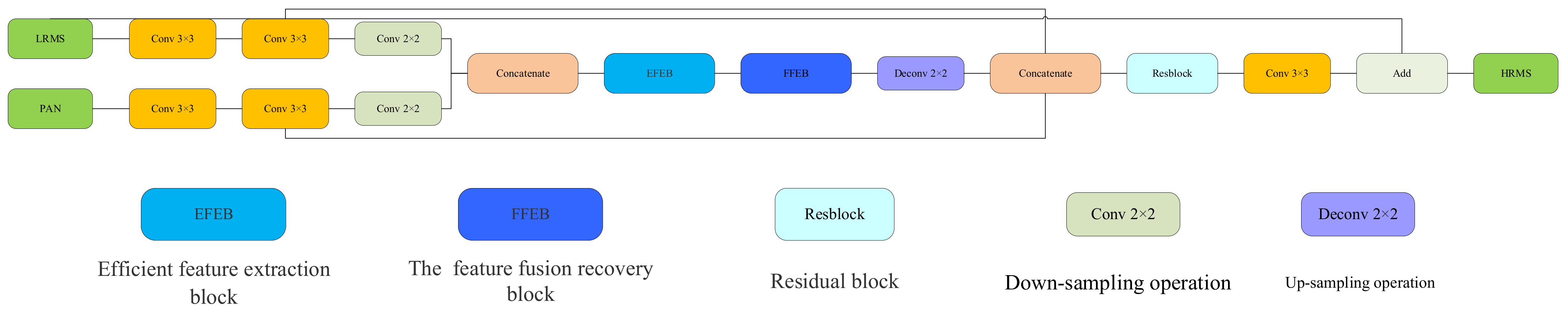
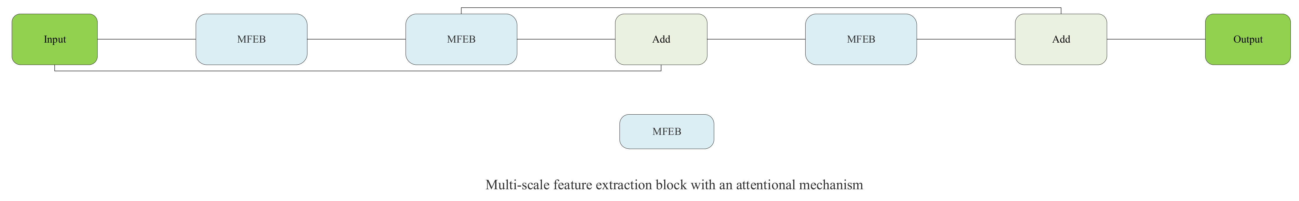
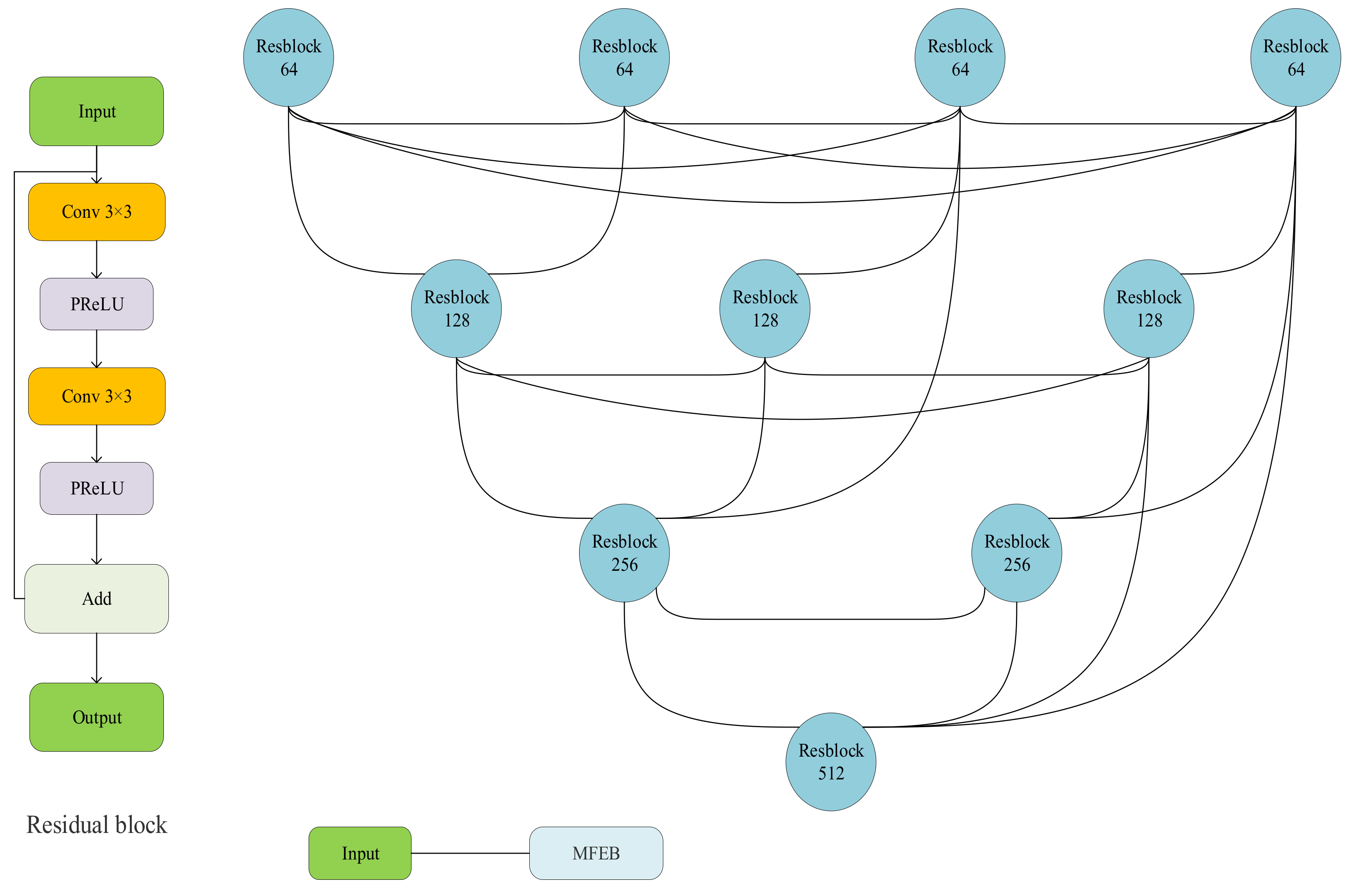
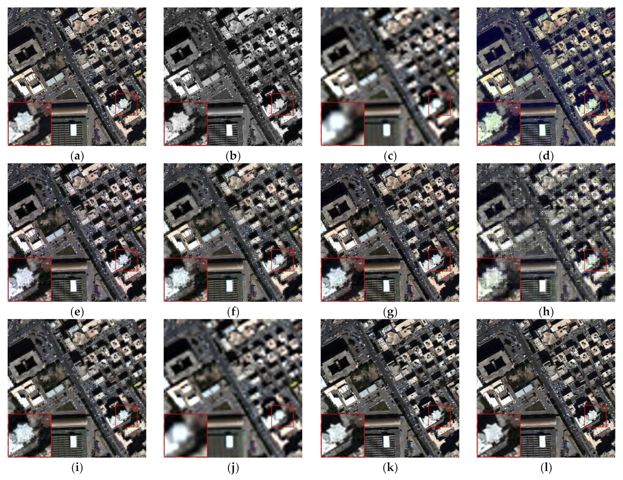
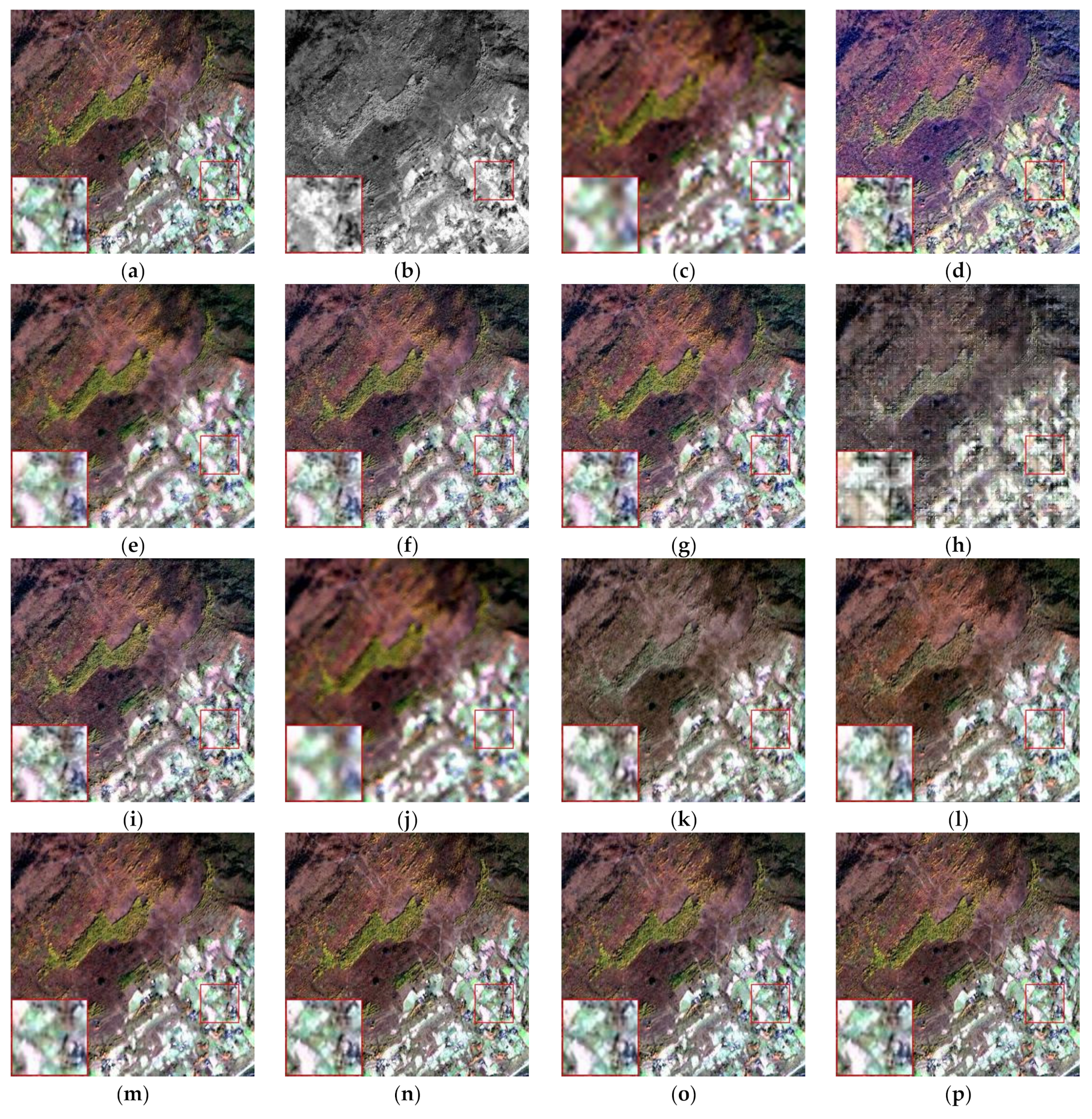
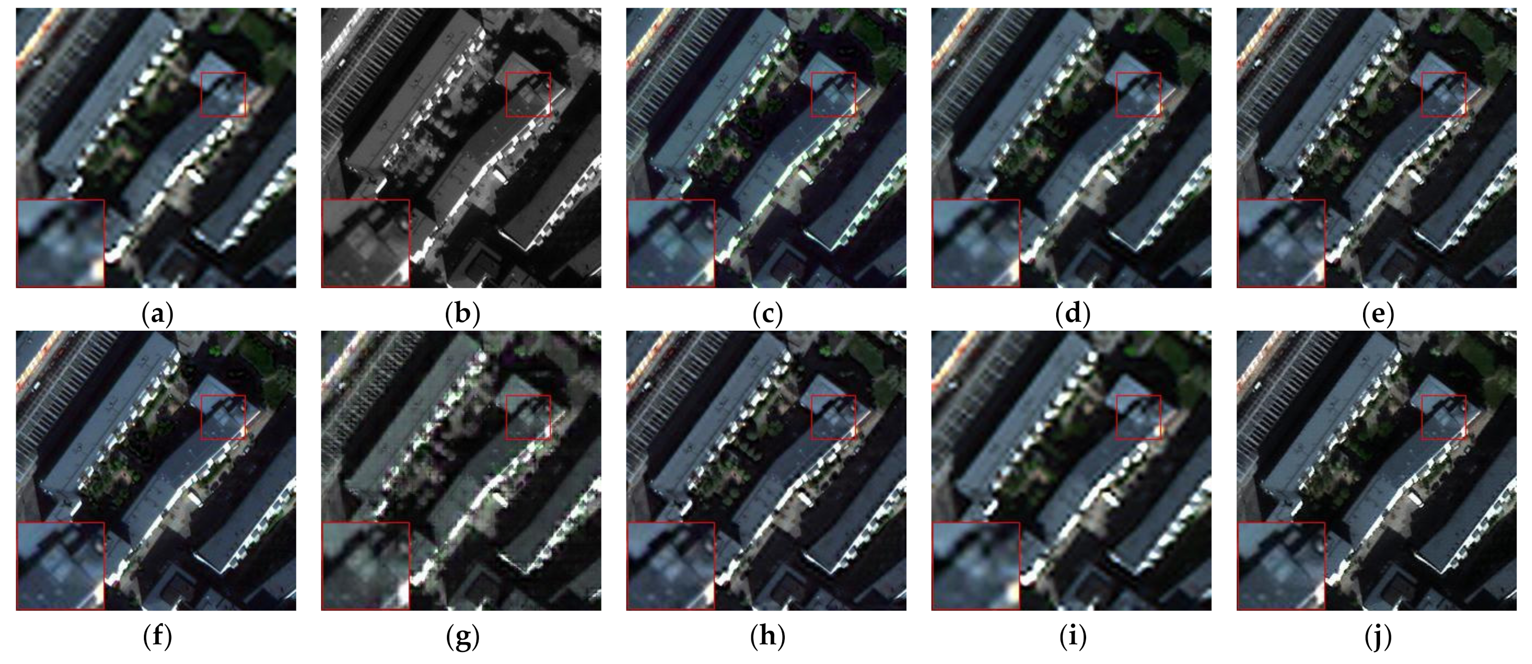
Table 1.
Size of training and test sets for different satellite datasets.
| Dataset | Total Numbers | Train Set | Validation Set |
|---|---|---|---|
| QuickBird | 950 | 750 | 200 |
| WorldView-2 | 750 | 600 | 150 |
| WorldView-3 | 1300 | 1000 | 300 |
| IKONOS | 160 | 144 | 16 |
Table 2.
Evaluations using the QuickBird dataset (best result is in bold).
| Method | SAM↓ | RASE↓ | Q_AVE↑ | ERGAS↓ | CC↑ | Q4↑ | SSIM↑ |
|---|---|---|---|---|---|---|---|
| IHS | 7.3370 | 29.2116 | 0.6930 | 7.7931 | 0.9245 | 0.8383 | 0.6968 |
| PRACS | 6.6502 | 27.0441 | 0.6985 | 7.2882 | 0.9287 | 0.8693 | 0.7003 |
| HPF | 6.1590 | 26.5007 | 0.7199 | 7.1123 | 0.9308 | 0.8795 | 0.7177 |
| GS | 6.7736 | 28.6871 | 0.6995 | 7.6727 | 0.9282 | 0.8421 | 0.7047 |
| DWT | 12.6372 | 39.1140 | 0.5688 | 9.9968 | 0.8361 | 0.7731 | 0.5492 |
| GLP | 6.2712 | 26.1510 | 0.7300 | 7.0190 | 0.9329 | 0.8872 | 0.7305 |
| PPXS | 6.3972 | 37.0457 | 0.4738 | 9.8349 | 0.8606 | 0.7126 | 0.4433 |
| PNN | 4.8988 | 20.4170 | 0.7949 | 5.4583 | 0.9612 | 0.9259 | 0.8060 |
| DRPNN | 4.0506 | 16.5490 | 0.8340 | 4.4543 | 0.9738 | 0.9527 | 0.8519 |
| PanNet | 3.8544 | 14.0295 | 0.8497 | 3.7743 | 0.9808 | 0.9627 | 0.8664 |
| ResTFNet | 2.9400 | 12.1735 | 0.8834 | 3.2852 | 0.9858 | 0.9739 | 0.9031 |
| TPNwFB | 2.5072 | 10.0468 | 0.9072 | 2.7214 | 0.9909 | 0.9822 | 0.9263 |
| ours | 1.7930 | 6.6668 | 0.9495 | 1.7914 | 0.9958 | 0.9913 | 0.9577 |
Table 3.
Evaluations using the WorldView-2 dataset (best result is in bold).
| Method | SAM↓ | RASE↓ | Q_AVE↑ | ERGAS↓ | CC↑ | Q4↑ | SSIM↑ |
|---|---|---|---|---|---|---|---|
| IHS | 5.6371 | 25.9189 | 0.7103 | 6.4711 | 0.9003 | 0.8176 | 0.6712 |
| PRACS | 4.9892 | 24.8504 | 0.7471 | 6.0704 | 0.9056 | 0.8615 | 0.7070 |
| HPF | 4.7316 | 23.7913 | 0.7413 | 5.8646 | 0.9115 | 0.8643 | 0.6950 |
| GS | 5.1635 | 25.6432 | 0.7210 | 6.3201 | 0.9030 | 0.8286 | 0.6827 |
| DWT | 8.0542 | 31.1777 | 0.6142 | 7.8327 | 0.8368 | 0.7677 | 0.5529 |
| GLP | 4.8826 | 23.4767 | 0.7563 | 5.7863 | 0.9163 | 0.8732 | 0.7124 |
| PPXS | 5.0452 | 29.1005 | 0.5384 | 7.2093 | 0.8638 | 0.7565 | 0.4580 |
| PNN | 4.4631 | 20.0271 | 0.8148 | 4.9370 | 0.9390 | 0.9055 | 0.7846 |
| DRPNN | 4.3753 | 19.8093 | 0.8161 | 4.8780 | 0.9404 | 0.9075 | 0.7851 |
| PanNet | 4.4901 | 20.6826 | 0.8078 | 5.1074 | 0.9343 | 0.9003 | 0.7765 |
| ResTFNet | 4.2802 | 18.9940 | 0.8213 | 4.6836 | 0.9447 | 0.9107 | 0.7912 |
| TPNwFB | 4.0258 | 17.9753 | 0.8413 | 4.4353 | 0.9505 | 0.9216 | 0.8124 |
| ours | 3.7506 | 16.5804 | 0.8643 | 4.0970 | 0.9584 | 0.9346 | 0.8407 |
Table 4.
Evaluations using the WorldView-3 dataset (best result is in bold).
| Method | SAM↓ | RASE↓ | Q_AVE↑ | ERGAS↓ | CC↑ | Q4↑ | SSIM↑ |
|---|---|---|---|---|---|---|---|
| IHS | 3.9227 | 20.0131 | 0.8249 | 5.0851 | 0.9532 | 0.9167 | 0.7991 |
| PRACS | 3.9758 | 17.9972 | 0.8500 | 4.4154 | 0.9577 | 0.9437 | 0.8194 |
| HPF | 3.3183 | 17.7482 | 0.8369 | 4.4816 | 0.9580 | 0.9407 | 0.8002 |
| GS | 3.5870 | 19.7825 | 0.8341 | 5.0001 | 0.9546 | 0.9229 | 0.8091 |
| DWT | 7.4893 | 29.8107 | 0.6770 | 7.5423 | 0.8853 | 0.8337 | 0.6257 |
| GLP | 3.3455 | 16.9436 | 0.8564 | 4.2733 | 0.9652 | 0.9489 | 0.8255 |
| PPXS | 3.5409 | 24.1764 | 0.7045 | 6.1892 | 0.9202 | 0.8763 | 0.6456 |
| PNN | 3.0606 | 11.3623 | 0.9219 | 2.8347 | 0.9828 | 0.9752 | 0.9095 |
| DRPNN | 2.9469 | 11.0848 | 0.9276 | 2.7820 | 0.9836 | 0.9774 | 0.9157 |
| PanNet | 2.6216 | 10.9912 | 0.9288 | 2.7574 | 0.9840 | 0.9773 | 0.9170 |
| ResTFNet | 2.6916 | 11.3202 | 0.9317 | 2.8295 | 0.9831 | 0.9764 | 0.9207 |
| TPNwFB | 2.6904 | 11.1373 | 0.9257 | 2.7867 | 0.9835 | 0.9769 | 0.9125 |
| ours | 2.4029 | 9.9737 | 0.9421 | 2.4939 | 0.9868 | 0.9813 | 0.9326 |
Table 5.
Evaluations using the IKONOS dataset (best result is in bold).
| Method | SAM↓ | RASE↓ | Q_AVE↑ | ERGAS↓ | CC↑ | Q4↑ | SSIM↑ |
|---|---|---|---|---|---|---|---|
| IHS | 3.1691 | 13.8400 | 0.3860 | 3.1599 | 0.9427 | 0.4741 | 0.4089 |
| PRACS | 2.8249 | 12.7932 | 0.4800 | 2.6011 | 0.9513 | 0.6675 | 0.5197 |
| HPF | 2.7730 | 13.5253 | 0.4683 | 2.7728 | 0.9458 | 0.6389 | 0.4950 |
| GS | 2.8089 | 14.0234 | 0.4487 | 2.8821 | 0.9411 | 0.6032 | 0.4896 |
| DWT | 9.4846 | 22.7378 | 0.3183 | 5.4503 | 0.8553 | 0.2945 | 0.3417 |
| GLP | 2.7788 | 13.5999 | 0.4852 | 2.8028 | 0.9455 | 0.6458 | 0.5083 |
| PPXS | 2.7693 | 12.7035 | 0.4065 | 2.5701 | 0.9535 | 0.6351 | 0.4725 |
| PNN | 2.4621 | 8.2089 | 0.7088 | 1.8787 | 0.9801 | 0.8057 | 0.7508 |
| DRPNN | 2.3908 | 8.6174 | 0.7147 | 1.9280 | 0.9786 | 0.8121 | 0.7521 |
| PanNet | 1.8269 | 5.6283 | 0.7899 | 1.3172 | 0.9909 | 0.8862 | 0.8210 |
| ResTFNet | 0.6309 | 1.4935 | 0.9512 | 0.4399 | 0.9994 | 0.9747 | 0.9659 |
| TPNwFB | 1.2008 | 3.3423 | 0.8842 | 0.8731 | 0.9968 | 0.9375 | 0.9069 |
| ours | 0.4096 | 1.0310 | 0.9680 | 0.2973 | 0.9997 | 0.9824 | 0.9802 |
Table 6.
Evaluations using the WorldView-3 Real Dataset (best result is in bold).
| Method | QNP↑ | Dλ↓ | Ds↓ |
|---|---|---|---|
| IHS | 0.6315 | 0.0794 | 0.3140 |
| PRACS | 0.8041 | 0.0287 | 0.1721 |
| HPF | 0.6710 | 0.1067 | 0.2488 |
| GS | 0.6426 | 0.0708 | 0.3084 |
| DWT | 0.6119 | 0.2875 | 0.1412 |
| GLP | 0.6755 | 0.1082 | 0.2425 |
| PPXS | 0.8936 | 0.0063 | 0.1008 |
| PNN | 0.7134 | 0.1080 | 0.2003 |
| DRPNN | 0.7515 | 0.0715 | 0.1907 |
| PanNet | 0.8052 | 0.0790 | 0.1257 |
| ResTFNet | 0.8805 | 0.0509 | 0.0723 |
| TPNwFB | 0.9116 | 0.0511 | 0.0393 |
| ours | 0.9213 | 0.0201 | 0.0598 |
Table 7.
Evaluations using the QuickBird Real Dataset (best result is in bold).
| Method | QNP↑ | Dλ↓ | Ds↓ |
|---|---|---|---|
| IHS | 0.6096 | 0.1173 | 0.3093 |
| PRACS | 0.8293 | 0.0374 | 0.1384 |
| HPF | 0.6468 | 0.1216 | 0.2636 |
| GS | 0.6418 | 0.0920 | 0.2932 |
| DWT | 0.5647 | 0.3273 | 0.1605 |
| GLP | 0.6512 | 0.1198 | 0.2601 |
| PPXS | 0.8743 | 0.0061 | 0.1203 |
| PNN | 0.7766 | 0.1871 | 0.0446 |
| DRPNN | 0.8178 | 0.0979 | 0.0935 |
| PanNet | 0.8236 | 0.0817 | 0.1031 |
| ResTFNet | 0.9211 | 0.0426 | 0.0379 |
| TPNwFB | 0.9090 | 0.0495 | 0.0437 |
| Proposed | 0.9311 | 0.0205 | 0.0494 |
Table 8.
Different deep learning methods for processing time and model size.
| Method | Time (S) | Model Size (MB) |
|---|---|---|
| PNN | 1.92 | 0.31 |
| DRPNN | 2.08 | 3.19 |
| PanNet | 2.22 | 2.06 |
| ResTFNet | 2.49 | 8.55 |
| TPNwFB | 2.82 | 52.3 |
| Proposed | 3.13 | 210 |
Table 9.
Quantitative evaluation results of multiscale feature-extraction modules with different combinations are shown in bold.
Table 9.
Quantitative evaluation results of multiscale feature-extraction modules with different combinations are shown in bold.
| Scale | SAM↓ | RASE↓ | Q_AVE↑ | ERGAS↓ | CC↑ | Q4↑ | SSIM↑ |
|---|---|---|---|---|---|---|---|
| 1123 | 2.0460 | 7.4101 | 0.9369 | 2.0083 | 0.9949 | 0.9897 | 0.9498 |
| 1124 | 2.0284 | 7.4482 | 0.9425 | 1.9891 | 0.9948 | 0.9899 | 0.9539 |
| 1125 | 2.1016 | 7.3502 | 0.9356 | 1.9812 | 0.9949 | 0.9897 | 0.9485 |
| 1223 | 2.1681 | 7.6609 | 0.9295 | 2.0630 | 0.9944 | 0.9890 | 0.9453 |
| 1224 | 2.2350 | 7.8802 | 0.9207 | 2.1199 | 0.9941 | 0.9879 | 0.9402 |
| 1225 | 2.0571 | 7.2789 | 0.9379 | 1.9671 | 0.9949 | 0.9903 | 0.9509 |
| 1233 | 1.9660 | 6.6951 | 0.9392 | 1.8075 | 0.9958 | 0.9913 | 0.9532 |
| 1234 | 1.7930 | 6.6668 | 0.9495 | 1.7914 | 0.9958 | 0.9913 | 0.9577 |
| 1235 | 1.8182 | 6.6792 | 0.9487 | 1.7930 | 0.9958 | 0.9914 | 0.9579 |
| 1333 | 2.1834 | 7.6122 | 0.9229 | 2.0516 | 0.9945 | 0.9889 | 0.9424 |
| 1334 | 1.9818 | 7.1717 | 0.9431 | 1.9291 | 0.9952 | 0.9906 | 0.9543 |
| 1335 | 2.2714 | 8.0409 | 0.9193 | 2.1526 | 0.9940 | 0.9879 | 0.9391 |
Table 10.
Quantitative evaluation results of different structures using different datasets. In A, a contrasting network without EFEB. In B, our network is used.
Table 10.
Quantitative evaluation results of different structures using different datasets. In A, a contrasting network without EFEB. In B, our network is used.
| Scale | SAM | RASE | Q_AVE | ERGAS | CC | Q4 | SSIM |
|---|---|---|---|---|---|---|---|
| QuickBird (A) | 2.4643 | 8.5049 | 0.9135 | 2.2910 | 0.9932 | 0.9863 | 0.9335 |
| QuickBird (B) | 1.7930 | 6.6668 | 0.9495 | 1.7914 | 0.9958 | 0.9913 | 0.9577 |
| WorldView-2 (A) | 3.8236 | 16.6670 | 0.8622 | 4.1180 | 0.9578 | 0.9332 | 0.8386 |
| WorldView-2 (B) | 3.7506 | 16.5804 | 0.8643 | 4.0970 | 0.9584 | 0.9346 | 0.8407 |
| WorldView-3 (A) | 2.4399 | 10.2544 | 0.9402 | 2.5637 | 0.9861 | 0.9804 | 0.9302 |
| WorldView-3 (B) | 2.4029 | 9.9737 | 0.9421 | 2.4939 | 0.9868 | 0.9813 | 0.9326 |
| IKONOS (A) | 0.4096 | 1.0310 | 0.9680 | 0.2973 | 0.9997 | 0.9824 | 0.9802 |
| IKONOS (B) | 0.6157 | 1.4487 | 0.9558 | 0.4389 | 0.9996 | 0.9831 | 0.9748 |
Table 11.
Quantitative evaluation results of different structures using different datasets. In A, a contrasting network is used. In B, our network is used.
Table 11.
Quantitative evaluation results of different structures using different datasets. In A, a contrasting network is used. In B, our network is used.
| Scale | SAM | RASE | Q_AVE | ERGAS | CC | Q4 | SSIM |
|---|---|---|---|---|---|---|---|
| QuickBird (A) | 2.8675 | 10.8443 | 0.8930 | 2.9372 | 0.9888 | 0.9788 | 0.9152 |
| QuickBird (B) | 1.7930 | 6.6668 | 0.9495 | 1.7914 | 0.9958 | 0.9913 | 0.9577 |
| WorldView-2 (A) | 3.8805 | 17.6535 | 0.8488 | 4.3531 | 0.9529 | 0.9260 | 0.8222 |
| WorldView-2 (B) | 3.7506 | 16.5804 | 0.8643 | 4.0970 | 0.9584 | 0.9346 | 0.8407 |
| WorldView-3 (A) | 2.4125 | 10.2680 | 0.9396 | 2.5737 | 0.9860 | 0.9803 | 0.9294 |
| WorldView-3 (B) | 2.4029 | 9.9737 | 0.9421 | 2.4939 | 0.9868 | 0.9813 | 0.9326 |
| IKONOS (A) | 0.7847 | 1.9036 | 0.9430 | 0.5412 | 0.9990 | 0.9689 | 0.9582 |
| IKONOS (B) | 0.6157 | 1.4487 | 0.9558 | 0.4389 | 0.9996 | 0.9831 | 0.9748 |
Table 12.
Results of the network quantitative evaluation with different iterations. The best performance is shown in bold.
Table 12.
Results of the network quantitative evaluation with different iterations. The best performance is shown in bold.
| Scale | SAM | RASE | Q_AVE | ERGAS | CC | Q4 | SSIM |
|---|---|---|---|---|---|---|---|
| 1 | 2.7088 | 9.1094 | 0.9039 | 2.4473 | 0.9923 | 0.9841 | 0.9276 |
| 2 | 2.4039 | 8.4655 | 0.9214 | 2.2745 | 0.9931 | 0.9861 | 0.9361 |
| 3 | 2.0831 | 7.3411 | 0.9402 | 1.9763 | 0.9948 | 0.9898 | 0.9509 |
| 4 | 1.7930 | 6.6668 | 0.9495 | 1.7914 | 0.9958 | 0.9913 | 0.9577 |
| 5 | 2.0550 | 7.1303 | 0.9379 | 1.9180 | 0.9952 | 0.9903 | 0.9504 |
Table 13.
Quantitative evaluation results of different structures using different datasets. In A, a contrasting network. In B, our network is used.
Table 13.
Quantitative evaluation results of different structures using different datasets. In A, a contrasting network. In B, our network is used.
| Scale | SAM | RASE | Q_AVE | ERGAS | CC | Q4 | SSIM |
|---|---|---|---|---|---|---|---|
| QuickBird (A) | 2.6883 | 8.7127 | 0.9040 | 2.3564 | 0.9927 | 0.9854 | 0.9274 |
| QuickBird (B) | 1.7930 | 6.6668 | 0.9495 | 1.7914 | 0.9958 | 0.9913 | 0.9577 |
| WorldView-2 (A) | 4.2092 | 18.5268 | 0.8379 | 4.5671 | 0.9489 | 0.9198 | 0.8102 |
| WorldView-2 (B) | 3.7506 | 16.5804 | 0.8643 | 4.0970 | 0.9584 | 0.9346 | 0.8407 |
| WorldView-3 (A) | 2.5027 | 9.9731 | 0.9384 | 2.4939 | 0.9869 | 0.9813 | 0.9284 |
| WorldView-3 (B) | 2.4029 | 9.9737 | 0.9421 | 2.4939 | 0.9868 | 0.9813 | 0.9326 |
| IKONOS (A) | 0.6362 | 1.6218 | 0.9557 | 0.4448 | 0.9993 | 0.9750 | 0.9691 |
| IKONOS (B) | 0.6157 | 1.4487 | 0.9558 | 0.4389 | 0.9996 | 0.9831 | 0.9748 |
Publisher’s Note: MDPI stays neutral with regard to jurisdictional claims in published maps and institutional affiliations. |
© 2021 by the authors. Licensee MDPI, Basel, Switzerland. This article is an open access article distributed under the terms and conditions of the Creative Commons Attribution (CC BY) license (https://creativecommons.org/licenses/by/4.0/).
Share and Cite
MDPI and ACS Style
Li, W.; Xiang, M.; Liang, X. A Dense Encoder–Decoder Network with Feedback Connections for Pan-Sharpening. Remote Sens. 2021, 13, 4505. https://0-doi-org.brum.beds.ac.uk/10.3390/rs13224505
AMA Style
Li W, Xiang M, Liang X. A Dense Encoder–Decoder Network with Feedback Connections for Pan-Sharpening. Remote Sensing. 2021; 13(22):4505. https://0-doi-org.brum.beds.ac.uk/10.3390/rs13224505
Chicago/Turabian StyleLi, Weisheng, Minghao Xiang, and Xuesong Liang. 2021. "A Dense Encoder–Decoder Network with Feedback Connections for Pan-Sharpening" Remote Sensing 13, no. 22: 4505. https://0-doi-org.brum.beds.ac.uk/10.3390/rs13224505
Note that from the first issue of 2016, this journal uses article numbers instead of page numbers. See further details here.