
Estimating Ground Elevation and Vegetation Characteristics in Coastal Salt Marshes Using UAV-Based LiDAR and Digital Aerial Photogrammetry

 , ,
, ,
Abstract
:1. Introduction
2. Data and Methods
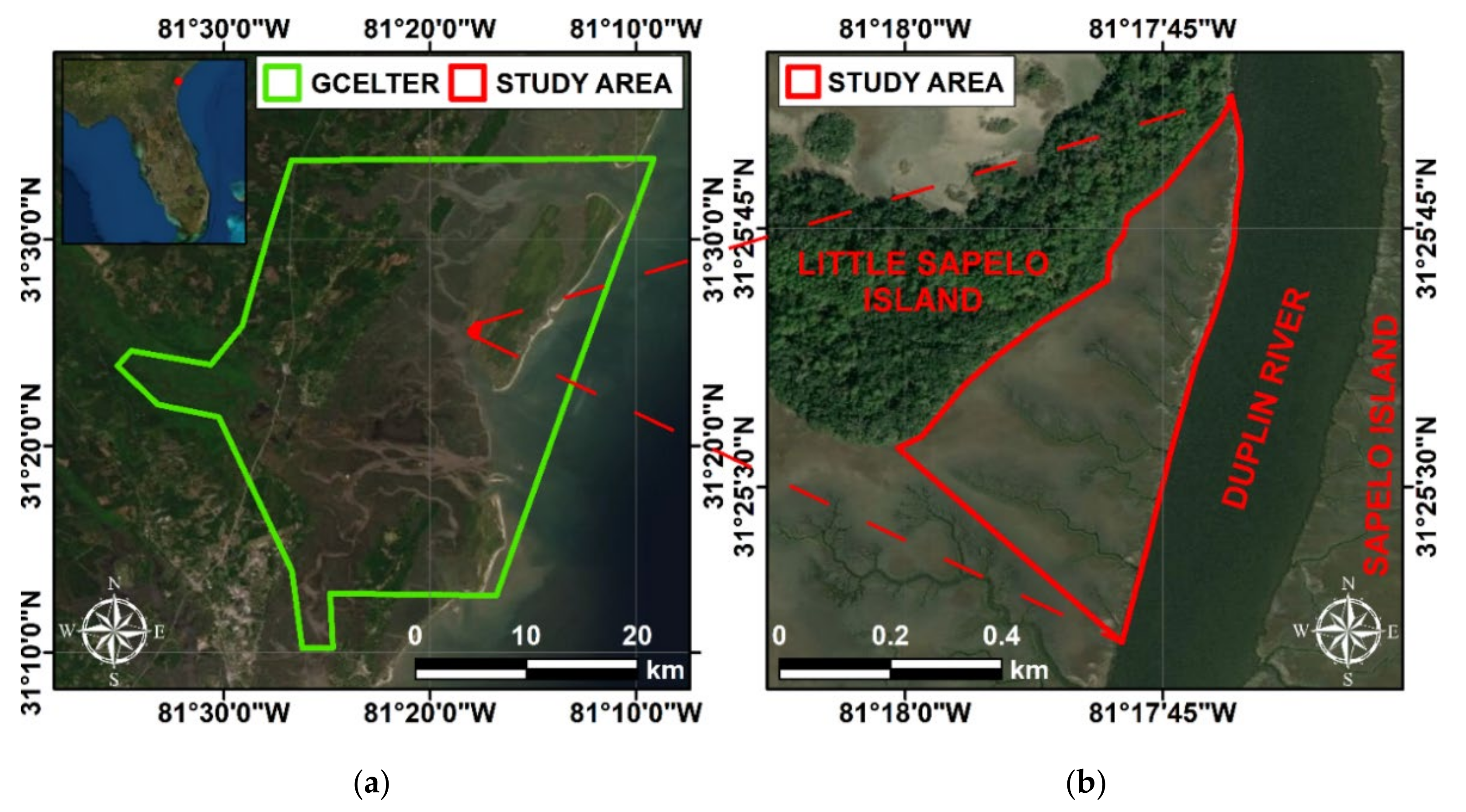
2.1. Study Site
2.2. Field Measurements
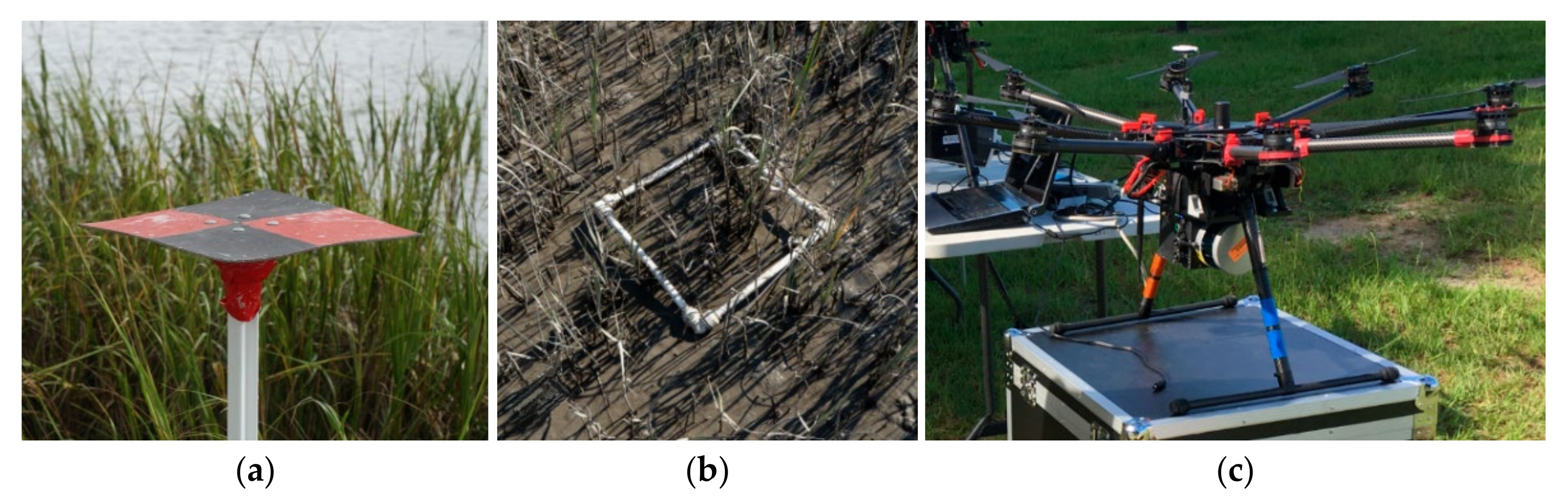
2.2.1. Ground Control Points
2.2.2. Ground Elevation and Vegetation Survey
2.3. Remote Sensing Survey
2.3.1. LiDAR-UAV Point Cloud
2.3.2. Imagery Dataset
2.3.3. Point Clouds Post-Processing
2.4. Ground Elevation and Vegetation Properties Estimation
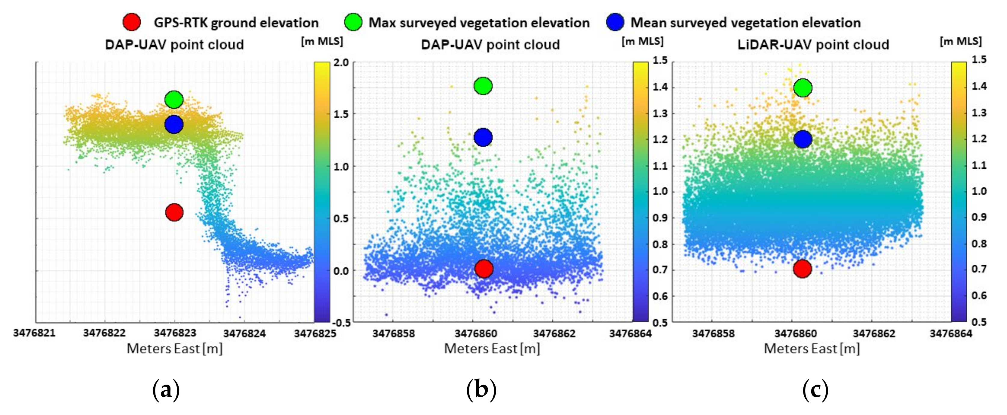
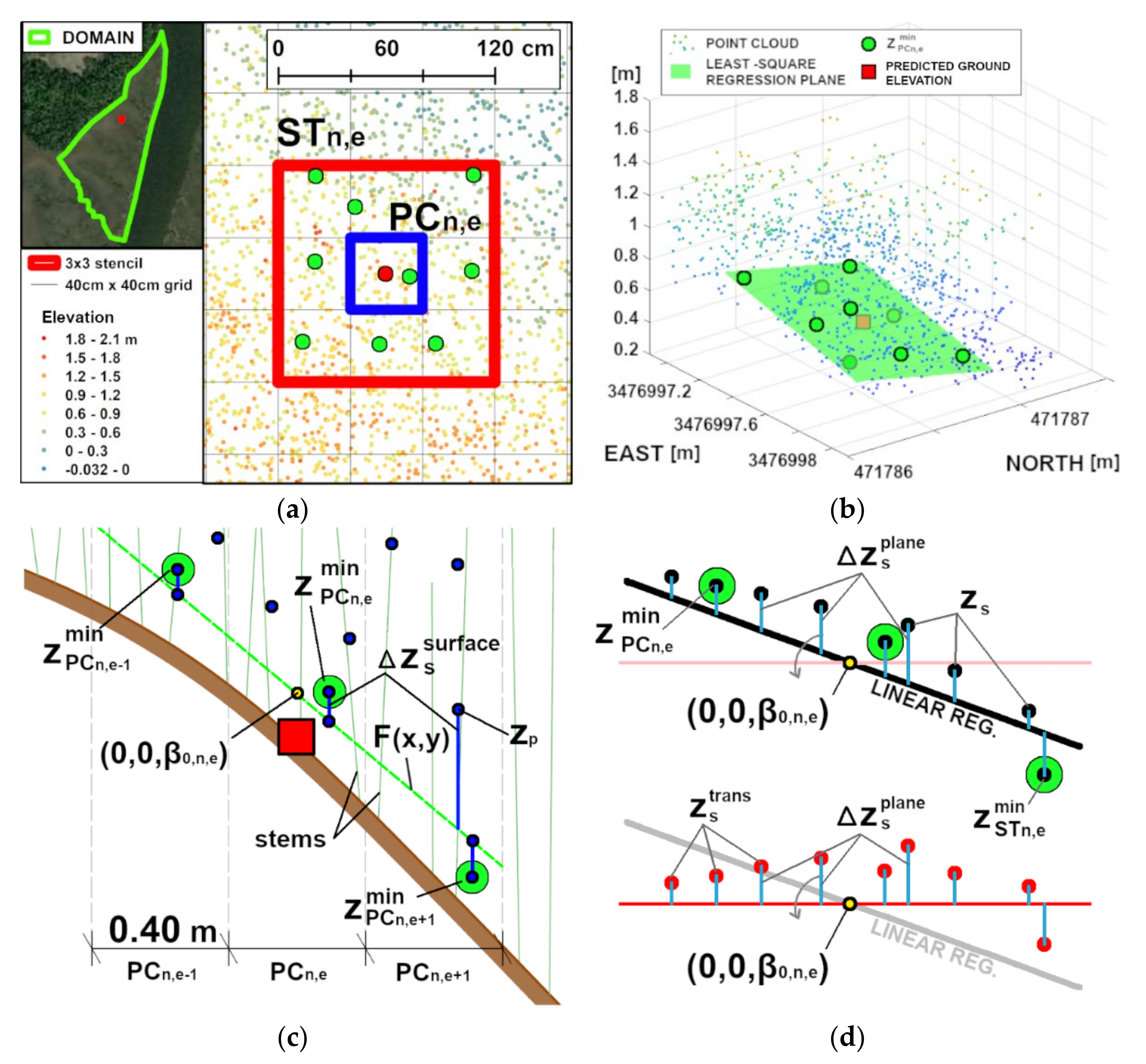
2.4.1. Point Cloud Transformation Algorithm
2.4.2. Genetic Algorithm
2.5. Leave-One-Out Cross-Validation Procedure
2.5.1. Model Predictors
2.5.2. Model Predictors from the Point Clouds
2.5.3. Model Predictors from the Imagery (RGB) Dataset
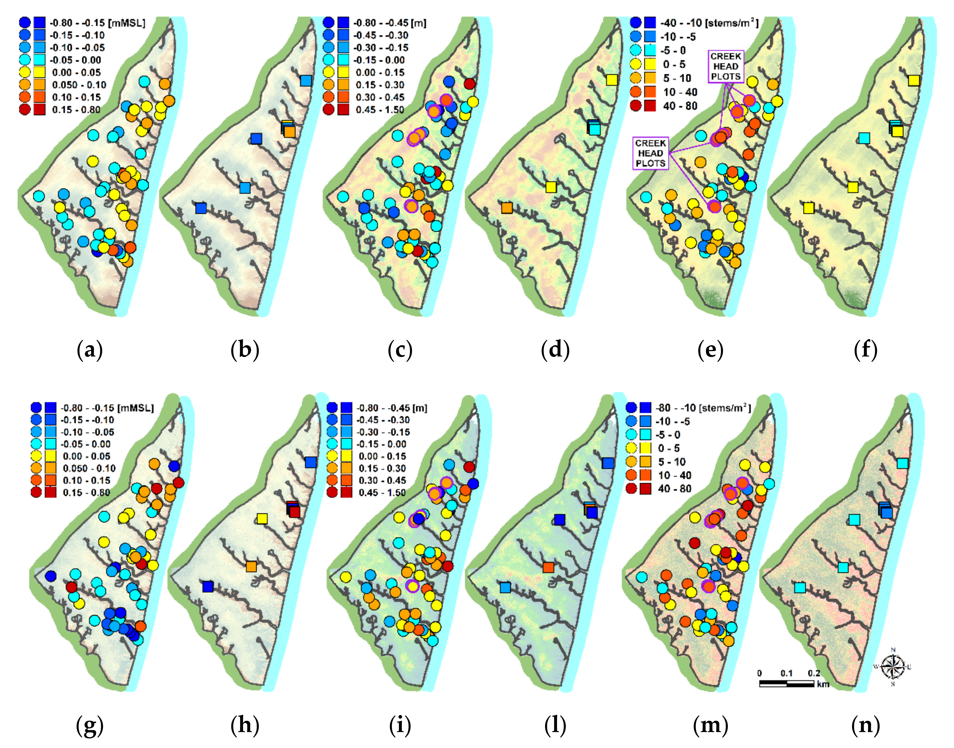
2.6. Error Analysis
3. Results
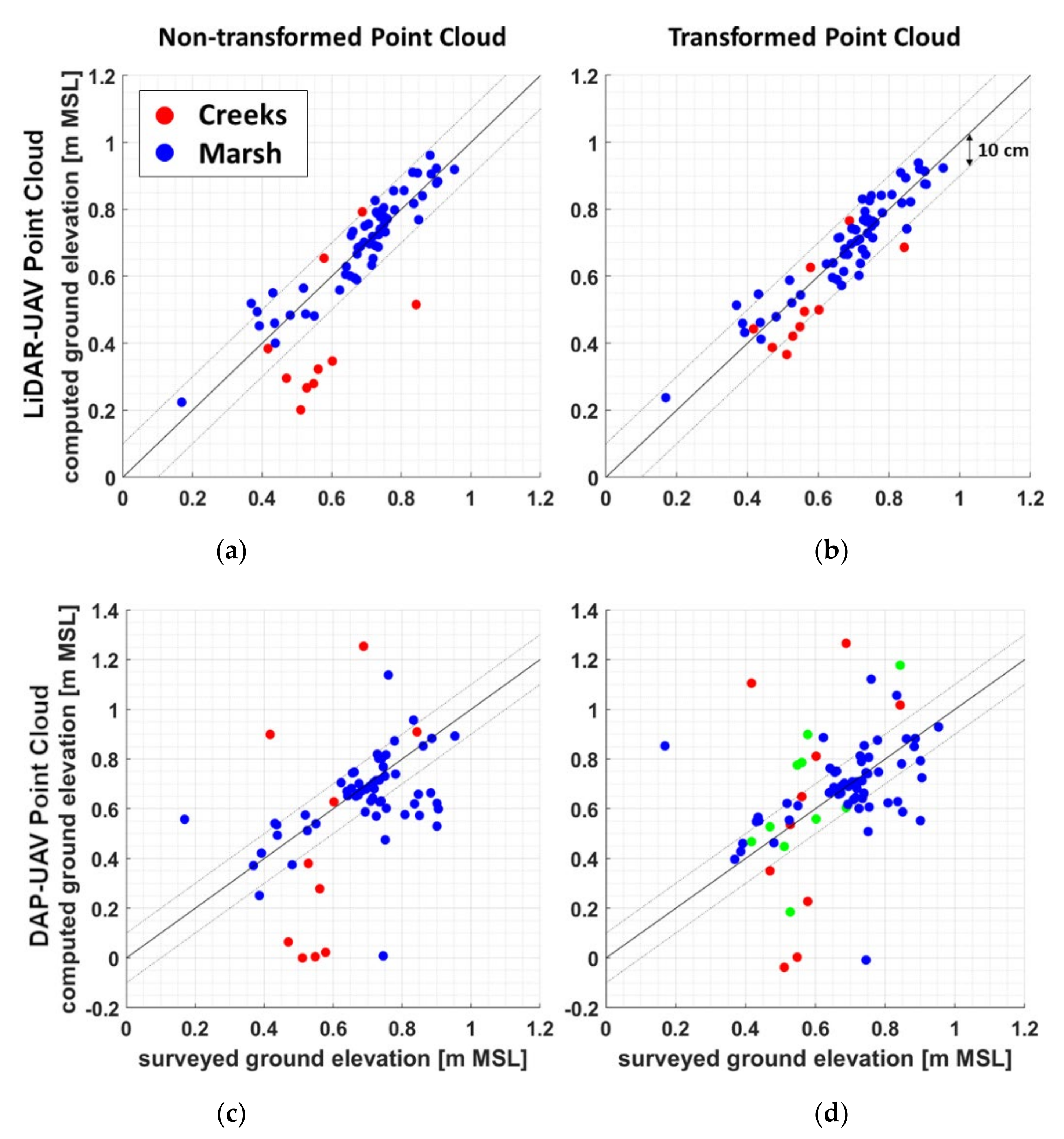
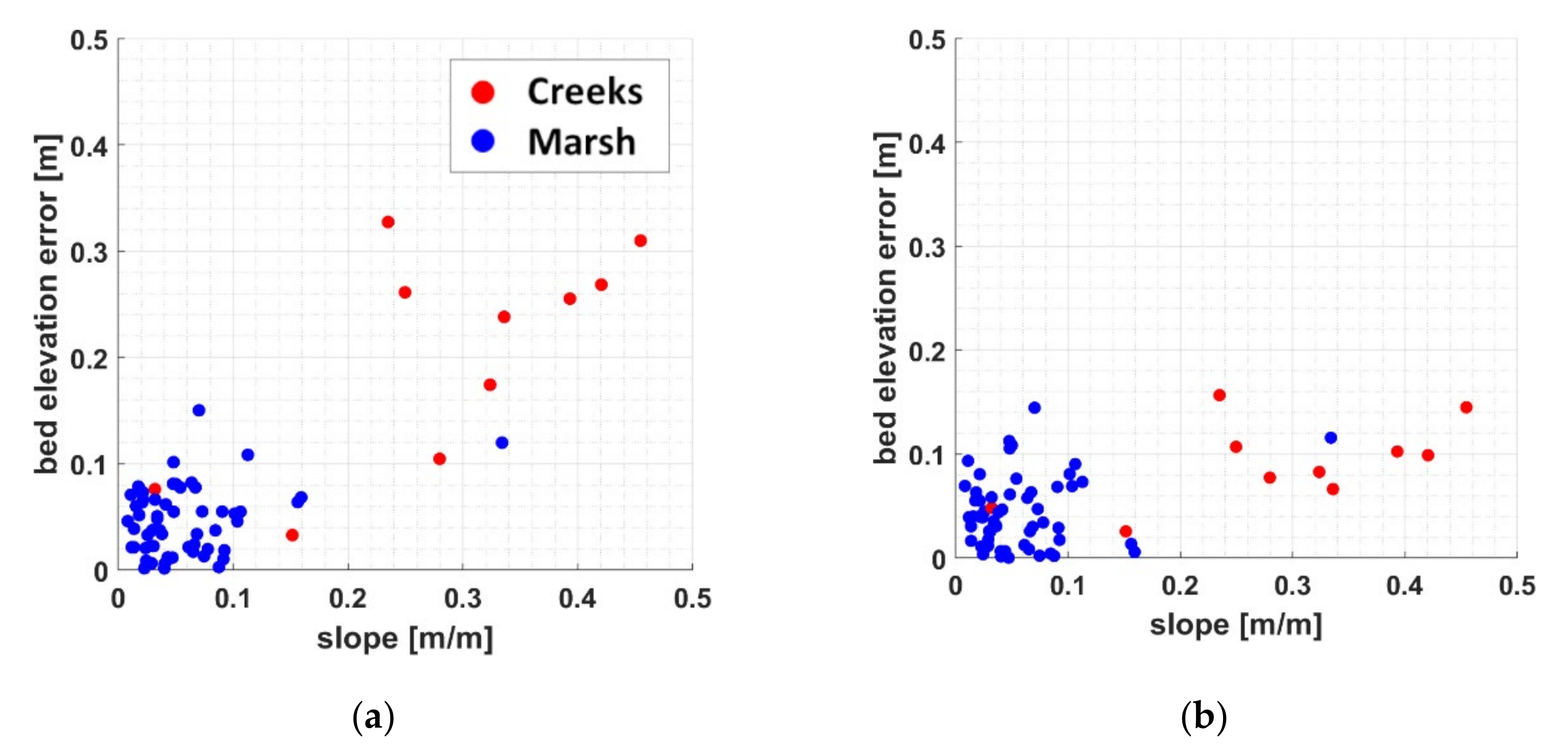
3.1. Ground Elevation Estimate
3.2. Vegetation Height and Density Estimates
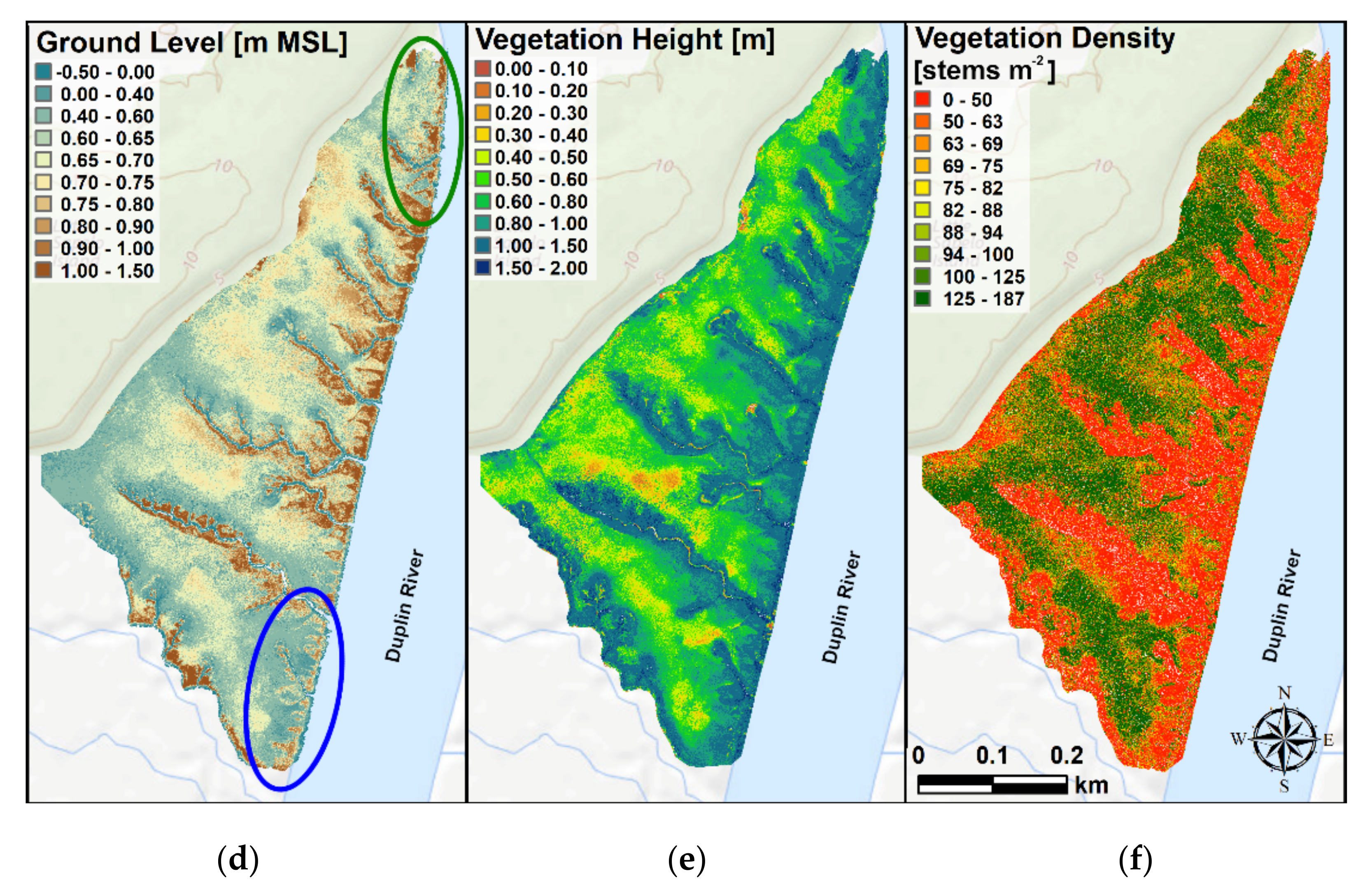
3.3. Ground Elevation and Vegetation Maps
4. Discussion
4.1. Ground Elevation Estimate
4.2. Vegetation Height and Density Estimate
4.3. High-Resolution Maps: LiDAR-UAV vs. DAP-UAV
4.4. Point Cloud Accuracy in the Literature
4.5. Limits of the Method
- Although our method detects vegetation characteristics remotely from a UAV, it requires active walking on the marsh to (i) position the land station used to calibrate the GNSS sensor on the drone, and (ii) survey bed elevations, vegetation height, and vegetation density, for calibration and validation purposes. The first limitation can be reduced by positioning the station at the boundary of the survey area, limiting the trampling to a very restricted area of the marsh. The second limit could be only partially bypassed by surveying ground elevation from a boat or a kayak, at the high tide. This method could not be used to survey vegetation properties because most of it is completely submerged during high tide. In conclusion, because this limitation could not be completely bypassed, its effects can be reduced by reducing the number of surveyed plots. Future research may be conducted to determine the error obtained by using datasets of different sizes and compositions to calibrate and validate our model.
- Due to the inability of our LiDAR sensor to collect data underwater, our approach is not used to determine the ground level and the vegetation characteristics in subtidal coastal areas. This is the reason for the missing outputs in Figure 5. The missing values correspond to the portion of the creeks close to the main channel, where water is present even at low tide. This limitation could be bypassed by using dual-frequency laser scanners, which allow the detection of both topography and (underwater) bathymetry [110,111]. Especially in the main channel, where the water turbidity could reduce the performances of these dual-frequency LiDAR, the survey can be done by using Unmanned Underwater Vehicles (UUV). However, this technology is more expensive than the one used in standard topographic laser scanners, and their precision depends on water turbidity, which is generally high in our study area.
- The short (~20–30 minutes) battery life of the aircraft limits the usage of the method to relatively small areas. This limitation can be bypassed by using surrogate aircraft, such as ultralight aircraft. However, the use of these aircraft (i) requires adequate landing and take-off areas, such as an airport, reducing the flexibility of the survey obtained with vertical take-off and landing (VTOL) UAVs; (ii) is less stable than VTOL UAVs, thus complicating dataset collection and post-processing steps; (iii) requires human personal onboard, nullifying the reduction of human loss risk obtained using UAVs.
- A LiDAR survey requires the presence of a licensed and expert drone pilot to be performed, and the use of an adequate acquisition system (i.e., laser scanner). However, due to the great popularity drones are gaining in many fields, pilots’ availability is increasing, and the cost to recreate an acquisition system similar to the one we used is becoming more affordable.
5. Conclusions
Author Contributions
Funding
Institutional Review Board Statement
Informed Consent Statement
Data Availability Statement
Acknowledgments
Conflicts of Interest
Appendix A

References
- Pinton, D.; Xu, S.; Canestrelli, A. Managing Dyke Retreat: Importance of Channel Network Evolution and Mainland Slope on Storm Surge Dissipation Over Salt Marshes. AGU Fall Meeting 2020, 2020, EP061-0016. [Google Scholar]
- Stark, J.; Van Oyen, T.; Meire, P.; Temmerman, S. Observations of tidal and storm surge attenuation in a large tidal marsh. Limnol. Oceanogr. 2015, 60, 1371–1381. [Google Scholar] [CrossRef]
- Boesch, D.F.; Turner, R.E. Dependence of Fishery Species on Salt Marshes: The Role of Food and Refuge. Estuaries 1984, 7, 460–468. [Google Scholar] [CrossRef]
- Barbier, E.B.; Hacker, S.D.; Kennedy, C.; Koch, E.W.; Stier, A.; Silliman, B. The value of estuarine and coastal ecosystem services. Ecol. Monogr. 2011, 81, 169–193. [Google Scholar] [CrossRef]
- Pendleton, L.; Donato, D.C.; Murray, B.C.; Crooks, S.; Jenkins, W.A.; Sifleet, S.; Craft, C.B.; Fourqurean, J.; Kauffman, J.B.; Marbà, N.; et al. Estimating Global “Blue Carbon” Emissions from Conversion and Degradation of Vegetated Coastal Ecosystems. PLoS ONE 2012, 7, e43542. [Google Scholar] [CrossRef] [Green Version]
- Hardisky, M.A.; Gross, M.F.; Klemas, V. Remote Sensing of Coastal Wetlands. BioScience 1986, 36, 453–460. [Google Scholar] [CrossRef]
- Alizad, K.; Hagen, S.C.; Medeiros, S.C.; Bilskie, M.V.; Morris, J.T.; Balthis, L.; Buckel, C.A. Dynamic responses and implications to coastal wetlands and the surrounding regions under sea level rise. PLoS ONE 2018, 13, e0205176. [Google Scholar] [CrossRef]
- Day, J.W.; Kemp, G.P.; Reed, D.J.; Cahoon, D.R.; Boumans, R.M.; Suhayda, J.M.; Gambrell, R. Vegetation death and rapid loss of surface elevation in two contrasting Mississippi delta salt marshes: The role of sedimentation, autocompaction and sea-level rise. Ecol. Eng. 2011, 37, 229–240. [Google Scholar] [CrossRef]
- Morris, J.; Sundberg, K.; Hopkinson, C. Salt Marsh Primary Production and Its Responses to Relative Sea Level and Nutrients in Estuaries at Plum Island, Massachusetts, and North Inlet, South Carolina, USA. Oceanography 2013, 26, 78–84. [Google Scholar] [CrossRef]
- Kirwan, M.L.; Temmerman, S.; Skeehan, M.L.K.E.E.; Guntenspergen, G.R.; Fagherazzi, S. Overestimation of marsh vulnerability to sea level rise. Nat. Clim. Chang. 2016, 6, 253–260. [Google Scholar] [CrossRef]
- Saintilan, N.; Kovalenko, K.; Guntenspergen, G.; Rogers, K.; Lynch, J.; Cahoon, D.; Gamage, V.P. Global patterns and drivers of tidal marsh response to accelerating sea-level rise. Res. Sq. 2021. in review. [Google Scholar] [CrossRef]
- Mahdianpari, M.; Granger, J.E.; Mohammadimanesh, F.; Warren, S.; Puestow, T.; Salehi, B.; Brisco, B. Smart solutions for smart cities: Urban wetland mapping using very-high resolution satellite imagery and airborne LiDAR data in the City of St. John’s, NL, Canada. J. Environ. Manag. 2020, 280, 111676. [Google Scholar] [CrossRef] [PubMed]
- US Census Bureau. Coastline America No. June. 2019. Available online: https://www.census.gov/library/visualizations/2019/demo/coastline-america.html (accessed on 7 November 2020).
- Marani, M.; Belluco, E.; D’Alpaos, A.; Defina, A.; Lanzoni, S.; Rinaldo, A. On the drainage density of tidal networks. Water Resour. Res. 2003, 39, 1040. [Google Scholar] [CrossRef]
- Reed, D.J.; Cahoon, D.R. The relationship between marsh surface topography, hydroperiod, and growth of Spartina alterniflora in a deteriorating Louisiana salt marsh. J. Coast. Res. 1992, 8, 77–87. [Google Scholar]
- Beeson, C.; Doyle, P.F. Comparison of bank erosion at vegetated and non-vegetated channel bends. JAWRA J. Am. Water Resour. Assoc. 1995, 31, 983–990. [Google Scholar] [CrossRef]
- Peruzzo, P.; Viero, D.P.; Defina, A. A semi-empirical model to predict the probability of capture of buoyant particles by a cylindrical collector through capillarity. Adv. Water Resour. 2016, 97, 168–174. [Google Scholar] [CrossRef]
- Fagherazzi, S.; Kirwan, M.L.; Mudd, S.M.; Guntenspergen, G.T.; Temmerman, S.; D’Alpaos, A.; van de Koppel, J.; Rybczyk, J.M.; Reyes, E.; Craft, C.; et al. Numerical models of salt marsh evolution: Ecological, geomorphic, and climatic factors. Rev. Geophys. 2012, 50, RG1002. [Google Scholar] [CrossRef]
- Pinton, D.; Canestrelli, A.; Fantuzzi, L. A UAV-Based Dye-Tracking Technique to Measure Surface Velocities over Tidal Channels and Salt Marshes. J. Mar. Sci. Eng. 2020, 8, 364. [Google Scholar] [CrossRef]
- Ashall, L.M.; Mulligan, R.P.; van Proosdij, D.; Poirier, E. Application and validation of a three-dimensional hydrodynamic model of a macrotidal salt marsh. Coast. Eng. 2016, 114, 35–46. [Google Scholar] [CrossRef]
- Mariotti, G.; Canestrelli, A. Long-term morphodynamics of muddy backbarrier basins: Fill in or empty out? Water Resour. Res. 2017, 53, 7029–7054. [Google Scholar] [CrossRef]
- Bennett, W.G.; Van Veelen, T.J.; Fairchild, T.P.; Griffin, J.N.; Karunarathna, H. Computational Modelling of the Impacts of Saltmarsh Management Interventions on Hydrodynamics of a Small Macro-Tidal Estuary. J. Mar. Sci. Eng. 2020, 8, 373. [Google Scholar] [CrossRef]
- Pinton, D.; Canestrelli, A.; Wilkinson, B.; Ifju, P.; Ortega, A. A new algorithm for estimating ground elevation and vegetation characteristics in coastal salt marshes from high-resolution UAV-based LiDAR point clouds. Earth Surf. Process. Landforms 2020, 45, 3687–3701. [Google Scholar] [CrossRef]
- Rogers, J.N.; Parrish, C.E.; Ward, L.G.; Burdick, D.M. Evaluation of field-measured vertical obscuration and full waveform lidar to assess salt marsh vegetation biophysical parameters. Remote. Sens. Environ. 2015, 156, 264–275. [Google Scholar] [CrossRef]
- Silvestri, S.; Marani, M. Salt-Marsh Vegetation and Morphology: Basic Physiology, Modelling and Remote Sensing Observations. In The Ecogeomorphology of Tidal Marshes; American Geophysical Union: Washington, DC, USA, 2013; Volume 59, pp. 5–25. [Google Scholar] [CrossRef]
- Gross, M.F.; Hardisky, M.A.; Klemas, V. Applications to coastal wetlands vegetation. In Theory and Applications of Optical Remote Sensing; John Wiley Sons: New York, NY, USA, 1989; pp. 474–490. [Google Scholar]
- Zhang, M.; Ustin, S.L.; Rejmankova, E.; Sanderson, E.W. Monitoring Pacific coast salt marshes using remote sensing. Ecol. Appl. 1997, 7, 1039–1053. [Google Scholar] [CrossRef]
- Young, N.E.; Anderson, R.S.; Chignell, S.M.; Vorster, A.G.; Lawrence, R.; Evangelista, P.H. A survival guide to Landsat preprocessing. Ecology 2017, 98, 920–932. [Google Scholar] [CrossRef] [Green Version]
- Hardanto, A.; Mustofa, A. Crop stage classification using supervised algorithm based on UAV and Landsat 8 image. IOP Conf. Ser. Earth Environ. Sci. 2021, 653, 012102. [Google Scholar] [CrossRef]
- Murugan, D.; Garg, A.; Singh, D. Development of an Adaptive Approach for Precision Agriculture Monitoring with Drone and Satellite Data. IEEE J. Sel. Top. Appl. Earth Obs. Remote Sens. 2017, 10, 5322–5328. [Google Scholar] [CrossRef]
- Guo, M.; Li, J.; Sheng, C.; Xu, J.; Wu, L. A Review of Wetland Remote Sensing. Sensors 2017, 17, 777. [Google Scholar] [CrossRef] [Green Version]
- Moeslund, J.E.; Arge, L.; Bøcher, P.K.; Nygaard, B.; Svenning, J.-C. Geographically Comprehensive Assessment of Salt-Meadow Vegetation-Elevation Relations Using LiDAR. Wetlands 2011, 31, 471–482. [Google Scholar] [CrossRef]
- Pinton, D.; Canestrelli, A.; Angelini, C.; Wilkinson, B.; Ifju, P.; Ortega, A. Estimating the spatial distribution of vegetation height and ground level elevation in a mesotidal salt marsh from UAV LiDAR derived point cloud. In Proceedings of the GEOMORPHOMETRY, Perugia, Italy, 22–26 June 2020; p. 115. [Google Scholar] [CrossRef]
- Uysal, M.; İlçi, V.; Ozulu, İ.M.; Erol, S.; Alkan, R.M. 3D Shoreline Mapping Using an Unmanned Aerial Vehicle where. FIG Congr. 2018, 2018, 115. [Google Scholar]
- Alizad, K.; Medeiros, S.; Foster-Martinez, M.R.; Hagen, S.C. Model Sensitivity to Topographic Uncertainty in Meso- and Microtidal Marshes. IEEE J. Sel. Top. Appl. Earth Obs. Remote Sens. 2020, 13, 807–814. [Google Scholar] [CrossRef]
- Raber, G.T.; Schill, S.R. A low-cost small unmanned surface vehicle (sUSV) for very high-resolution mapping and monitoring of shallow marine habitats. Remote Sens. Ocean. Sea Ice Coast. Waters Large Water Reg. 2019, 11150, 1115004. [Google Scholar] [CrossRef]
- Grenzdörffer, G.J.; Engel, A.; Teichert, B.; Kumar, G.; Madison, W.D.S.; Madison, W.D.S.; Madison, W.D.S. UAVs in Agriculture: Perceptions, Prospects, and "Probably Not". Int. Arch. Photogramm. Remote. Sens. Spat. Inf. Sci. 2008, 1, 1207–1213. [Google Scholar]
- Gašparović, M.; Zrinjski, M.; Barković, Đ.; Radočaj, D. An automatic method for weed mapping in oat fields based on UAV imagery. Comput. Electron. Agric. 2020, 173, 105385. [Google Scholar] [CrossRef]
- Matese, A.; Toscano, P.; Di Gennaro, S.F.; Genesio, L.; Vaccari, F.P.; Primicerio, J.; Belli, C.; Zaldei, A.; Bianconi, R.; Gioli, B. Intercomparison of UAV, Aircraft and Satellite Remote Sensing Platforms for Precision Viticulture. Remote Sens. 2015, 7, 2971–2990. [Google Scholar] [CrossRef] [Green Version]
- Nie, S.; Wang, C.; Xi, X.; Luo, S.; Li, S.; Tian, J. Estimating the height of wetland vegetation using airborne discrete-return LiDAR data. Optik 2018, 154, 267–274. [Google Scholar] [CrossRef]
- Liu, H.; Dong, P.; Wu, C.; Wang, P.; Fang, M. Individual tree identification using a new cluster-based approach with discrete-return airborne LiDAR data. Remote Sens. Environ. 2021, 258, 112382. [Google Scholar] [CrossRef]
- Yun, T.; Jiang, K.; Li, G.; Eichhorn, M.P.; Fan, J.; Liu, F.; Chen, B.; An, F.; Cao, L. Individual tree crown segmentation from airborne LiDAR data using a novel Gaussian filter and energy function minimization-based approach. Remote Sens. Environ. 2021, 256, 112307. [Google Scholar] [CrossRef]
- Michałowska, M.; Rapiński, J. A Review of Tree Species Classification Based on Airborne LiDAR Data and Applied Classifiers. Remote Sens. 2021, 13, 353. [Google Scholar] [CrossRef]
- Chamberlain, C.P.; Meador, A.J.S.; Thode, A.E. Airborne lidar provides reliable estimates of canopy base height and canopy bulk density in southwestern ponderosa pine forests. For. Ecol. Manag. 2020, 481, 118695. [Google Scholar] [CrossRef]
- Richardson, M.C.; Mitchell, C.P.J.; Branfireun, B.A.; Kolka, R.K. Analysis of airborne LiDAR surveys to quantify the characteristic morphologies of northern forested wetlands. J. Geophys. Res. Space Phys. 2010, 115, G03005. [Google Scholar] [CrossRef] [Green Version]
- Huang, C.; Peng, Y.; Lang, M.; Yeo, I.-Y.; McCarty, G. Wetland inundation mapping and change monitoring using Landsat and airborne LiDAR data. Remote Sens. Environ. 2014, 141, 231–242. [Google Scholar] [CrossRef]
- Varin, M.; Bournival, P.; Fink, J.; Chalghaf, B. Mapping Vernal Pools Using LiDAR Data and Multitemporal Satellite Imagery. Wetlands 2021, 41, 1–15. [Google Scholar] [CrossRef]
- Hirano, A.; Madden, M.; Welch, R. Hyperspectral image data for mapping wetland vegetation. Wetlands 2003, 23, 436–448. [Google Scholar] [CrossRef]
- Wang, J.; Liu, Z.; Yu, H.; Li, F. Mapping Spartina alterniflora Biomass Using LiDAR and Hyperspectral Data. Remote Sens. 2017, 9, 589. [Google Scholar] [CrossRef] [Green Version]
- Pavri, F.; Dailey, A.; Valentine, V. Integrating multispectral ASTER and LiDAR data to characterize coastal wetland landscapes in the northeastern United States. Geocarto Int. 2011, 26, 647–661. [Google Scholar] [CrossRef]
- Rapinel, S.; Hubert-Moy, L.; Clément, B. Combined use of LiDAR data and multispectral earth observation imagery for wetland habitat mapping. Int. J. Appl. Earth Obs. Geoinf. 2015, 37, 56–64. [Google Scholar] [CrossRef]
- O’Neil, G.L.; Goodall, J.L.; Behl, M.; Saby, L. Deep learning Using Physically-Informed Input Data for Wetland Identification. Environ. Model. Softw. 2020, 126, 104665. [Google Scholar] [CrossRef]
- Bork, E.W.; Su, J.G. Integrating LIDAR data and multispectral imagery for enhanced classification of rangeland vegetation: A meta analysis. Remote Sens. Environ. 2007, 111, 11–24. [Google Scholar] [CrossRef]
- Moffett, K.B.; Gorelick, S.M. Distinguishing wetland vegetation and channel features with object-based image segmentation. Int. J. Remote Sens. 2012, 34, 1332–1354. [Google Scholar] [CrossRef]
- Schut, A.G.T.; Wardell-Johnson, G.W.; Yates, C.J.; Keppel, G.; Baran, I.; Franklin, S.E.; Hopper, S.D.; Van Niel, K.P.; Mucina, L.; Byrne, M. Rapid Characterisation of Vegetation Structure to Predict Refugia and Climate Change Impacts across a Global Biodiversity Hotspot. PLoS ONE 2014, 9, e82778. [Google Scholar] [CrossRef] [Green Version]
- Chen, C.; Chang, B.; Li, Y.; Shi, B. Filtering airborne LiDAR point clouds based on a scale-irrelevant and terrain-adaptive approach. Measurement 2020, 171, 108756. [Google Scholar] [CrossRef]
- Hartley, R.; Leonardo, E.; Massam, P.; Watt, M.; Estarija, H.; Wright, L.; Melia, N.; Pearse, G. An Assessment of High-Density UAV Point Clouds for the Measurement of Young Forestry Trials. Remote Sens. 2020, 12, 4039. [Google Scholar] [CrossRef]
- Mandlburger, G.; Pfennigbauer, M.; Riegl, U.; Haring, A.; Wieser, M.; Glira, P.; Winiwarter, L. Complementing airborne laser bathymetry with UAV-based lidar for capturing alluvial landscapes. Remote Sens. Agric. Ecosyst. Hydrol. 2015, 9637, 96370A. [Google Scholar] [CrossRef]
- Coveney, S.; Fotheringham, A.S. Terrestrial laser scan error in the presence of dense ground vegetation. Photogramm. Rec. 2011, 26, 307–324. [Google Scholar] [CrossRef] [Green Version]
- Ashcroft, M.B.; Gollan, J.R.; Ramp, D. Creating vegetation density profiles for a diverse range of ecological habitats using terrestrial laser scanning. Methods Ecol. Evol. 2014, 5, 263–272. [Google Scholar] [CrossRef] [Green Version]
- Nouwakpo, S.K.; Weltz, M.A.; McGwire, K. Assessing the performance of structure-from-motion photogrammetry and terrestrial LiDAR for reconstructing soil surface microtopography of naturally vegetated plots. Earth Surf. Process. Landforms 2015, 41, 308–322. [Google Scholar] [CrossRef]
- Kalacska, M.; Chmura, G.; Lucanus, O.; Bérubé, D.; Arroyo-Mora, J. Structure from motion will revolutionize analyses of tidal wetland landscapes. Remote Sens. Environ. 2017, 199, 14–24. [Google Scholar] [CrossRef]
- Gomez, C.; Hayakawa, Y.; Obanawa, H. A study of Japanese landscapes using structure from motion derived DSMs and DEMs based on historical aerial photographs: New opportunities for vegetation monitoring and diachronic geomorphology. Geomorphology 2015, 242, 11–20. [Google Scholar] [CrossRef] [Green Version]
- Comba, L.; Biglia, A.; Aimonino, D.R.; Gay, P. Unsupervised detection of vineyards by 3D point-cloud UAV photogrammetry for precision agriculture. Comput. Electron. Agric. 2018, 155, 84–95. [Google Scholar] [CrossRef]
- Shashi, M.; Jain, K. Use of Photogrammetry in 3D modeling and visualization of buildings. J. Eng. Appl. Sci. 2007, 2, 37–40. [Google Scholar]
- Cunliffe, A.M.; Brazier, R.E.; Anderson, K. Ultra-fine grain landscape-scale quantification of dryland vegetation structure with drone-acquired structure-from-motion photogrammetry. Remote Sens. Environ. 2016, 183, 129–143. [Google Scholar] [CrossRef] [Green Version]
- Fawcett, D.; Azlan, B.; Hill, T.C.; Kho, L.K.; Bennie, J.; Anderson, K. Unmanned aerial vehicle (UAV) derived structure-from-motion photogrammetry point clouds for oil palm (Elaeis guineensis) canopy segmentation and height estimation. Int. J. Remote Sens. 2019, 40, 7538–7560. [Google Scholar] [CrossRef] [Green Version]
- Stal, C.; Tack, F.; de Maeyer, P.; de Wulf, A.; Goossens, R. Airborne photogrammetry and lidar for DSM extraction and 3D change detection over an urban area – a comparative study. Int. J. Remote Sens. 2012, 34, 1087–1110. [Google Scholar] [CrossRef] [Green Version]
- James, M.; Robson, S. Straightforward reconstruction of 3D surfaces and topography with a camera: Accuracy and geoscience application. J. Geophys. Res. Space Phys. 2012, 117. [Google Scholar] [CrossRef] [Green Version]
- Järnstedt, J.; Pekkarinen, A.; Tuominen, S.; Ginzler, C.; Holopainen, M.; Viitala, R. Forest variable estimation using a high-resolution digital surface model. ISPRS J. Photogramm. Remote Sens. 2012, 74, 78–84. [Google Scholar] [CrossRef]
- White, J.C.; Wulder, M.A.; Vastaranta, M.; Coops, N.C.; Pitt, D.; Woods, M. The Utility of Image-Based Point Clouds for Forest Inventory: A Comparison with Airborne Laser Scanning. Forests 2013, 4, 518–536. [Google Scholar] [CrossRef] [Green Version]
- Filippelli, S.K.; Lefsky, M.A.; Rocca, M.E. Comparison and integration of lidar and photogrammetric point clouds for mapping pre-fire forest structure. Remote Sens. Environ. 2019, 224, 154–166. [Google Scholar] [CrossRef]
- Moudrý, V.; Gdulová, K.; Fogl, M.; Klápště, P.; Urban, R.; Komárek, J.; Moudrá, L.; Štroner, M.; Barták, V.; Solský, M. Comparison of leaf-off and leaf-on combined UAV imagery and airborne LiDAR for assessment of a post-mining site terrain and vegetation structure: Prospects for monitoring hazards and restoration success. Appl. Geogr. 2019, 104, 32–41. [Google Scholar] [CrossRef]
- Gatziolis, D.; Lienard, J.F.; Vogs, A.; Strigul, N.S. 3D Tree Dimensionality Assessment Using Photogrammetry and Small Unmanned Aerial Vehicles. PLoS ONE 2015, 10, e0137765. [Google Scholar] [CrossRef] [Green Version]
- Klápště, P.; Fogl, M.; Barták, V.; Gdulová, K.; Urban, R.; Moudrý, V. Sensitivity analysis of parameters and contrasting performance of ground filtering algorithms with UAV photogrammetry-based and LiDAR point clouds. Int. J. Digit. Earth 2020, 13, 1672–1694. [Google Scholar] [CrossRef]
- St-Onge, B.; Vega, C.; Fournier, R.A.; Hu, Y. Mapping canopy height using a combination of digital stereo-photogrammetry and lidar. Int. J. Remote Sens. 2008, 29, 3343–3364. [Google Scholar] [CrossRef]
- Noordermeer, L.; Bollandsås, O.M.; Ørka, H.O.; Næsset, E.; Gobakken, T. Comparing the accuracies of forest attributes predicted from airborne laser scanning and digital aerial photogrammetry in operational forest inventories. Remote Sens. Environ. 2019, 226, 26–37. [Google Scholar] [CrossRef]
- Song, H.; Yang, C.; Zhang, J.; Hoffmann, W.C.; He, D.; Thomasson, J.A. Comparison of mosaicking techniques for airborne images from consumer-grade cameras. J. Appl. Remote Sens. 2016, 10, 16030. [Google Scholar] [CrossRef] [Green Version]
- DiGiacomo, A.; Bird, C.; Pan, V.; Dobroski, K.; Atkins-Davis, C.; Johnston, D.; Ridge, J. Modeling Salt Marsh Vegetation Height Using Unoccupied Aircraft Systems and Structure from Motion. Remote Sens. 2020, 12, 2333. [Google Scholar] [CrossRef]
- Gil, A.L.; Núñez-Casillas, L.; Isenburg, M.; Benito, A.A.; Bello, J.J.R.; Arbelo, M. A comparison between LiDAR and photogrammetry digital terrain models in a forest area on Tenerife Island. Can. J. Remote Sens. 2013, 39, 396–409. [Google Scholar] [CrossRef]
- Cao, L.; Liu, H.; Fu, X.; Zhang, Z.; Shen, X.; Ruan, H. Comparison of UAV LiDAR and Digital Aerial Photogrammetry Point Clouds for Estimating Forest Structural Attributes in Subtropical Planted Forests. Forests 2019, 10, 145. [Google Scholar] [CrossRef] [Green Version]
- Kopyść, P.T. The use of aerial lidar and structure from motion (sfm) photogrammetry data in analyzing microtopographic changes on hiking trails on the example of kielce (poland). Carpathian J. Earth Environ. Sci. 2020, 15, 461–470. [Google Scholar] [CrossRef]
- Guerra-Hernández, J.; Cosenza, D.N.; Rodriguez, L.C.E.; Silva, M.; Tomé, M.; Díaz-Varela, R.A.; Gonzalez-Ferreiro, E. Comparison of ALS- and UAV(SfM)-derived high-density point clouds for individual tree detection in Eucalyptus plantations. Int. J. Remote Sens. 2018, 39, 5211–5235. [Google Scholar] [CrossRef]
- Goodbody, T.R.; Coops, N.C.; Hermosilla, T.; Tompalski, P.; Pelletier, G. Vegetation Phenology Driving Error Variation in Digital Aerial Photogrammetrically Derived Terrain Models. Remote Sens. 2018, 10, 1554. [Google Scholar] [CrossRef] [Green Version]
- Graham, A.; Coops, N.C.; Wilcox, M.; Plowright, A. Evaluation of Ground Surface Models Derived from Unmanned Aerial Systems with Digital Aerial Photogrammetry in a Disturbed Conifer Forest. Remote Sens. 2019, 11, 84. [Google Scholar] [CrossRef] [Green Version]
- Guerra-Hernández, J.; González-Ferreiro, E.; Monleón, V.J.; Faias, S.P.; Tomé, M.; Díaz-Varela, R.A. Use of Multi-Temporal UAV-Derived Imagery for Estimating Individual Tree Growth in Pinus pinea Stands. Forests 2017, 8, 300. [Google Scholar] [CrossRef]
- Jensen, J.L.R.; Mathews, A.J. Assessment of Image-Based Point Cloud Products to Generate a Bare Earth Surface and Estimate Canopy Heights in a Woodland Ecosystem. Remote Sens. 2016, 8, 50. [Google Scholar] [CrossRef] [Green Version]
- Doughty, C.L.; Cavanaugh, K.C. Mapping Coastal Wetland Biomass from High Resolution Unmanned Aerial Vehicle (UAV) Imagery. Remote Sens. 2019, 11, 540. [Google Scholar] [CrossRef] [Green Version]
- Hladik, C.; Schalles, J.; Alber, M. Salt marsh elevation and habitat mapping using hyperspectral and LIDAR data. Remote Sens. Environ. 2013, 139, 318–330. [Google Scholar] [CrossRef]
- Schalles, J.; Hladik, C.; Lynes, A.; Pennings, S. Landscape Estimates of Habitat Types, Plant Biomass, and Invertebrate Densities in a Georgia Salt Marsh. Oceanography 2013, 26, 88–97. [Google Scholar] [CrossRef] [Green Version]
- Wiegert, R.G.; Chalmers, A.G.; Randerson, P.F. Productivity Gradients in Salt Marshes: The Response of Spartina alterniflora to Experimentally Manipulated Soil Water Movement. Oikos 1983, 41, 1–6. [Google Scholar] [CrossRef]
- Wang, D.; Xin, X.; Shao, Q.; Brolly, M.; Zhu, Z.; Chen, J. Modeling Aboveground Biomass in Hulunber Grassland Ecosystem by Using Unmanned Aerial Vehicle Discrete Lidar. Sensors 2017, 17, 180. [Google Scholar] [CrossRef] [PubMed] [Green Version]
- Canestrelli, A.; Spruyt, A.; Jagers, B.; Slingerland, R.; Borsboom, M. A mass-conservative staggered immersed boundary model for solving the shallow water equations on complex geometries. Int. J. Numer. Methods Fluids 2015, 81, 151–177. [Google Scholar] [CrossRef]
- Canestrelli, A.; Dumbser, M.; Siviglia, A.; Toro, E.F. Well-balanced high-order centered schemes on unstructured meshes for shallow water equations with fixed and mobile bed. Adv. Water Resour. 2010, 33, 291–303. [Google Scholar] [CrossRef]
- Madár, J.; Abonyi, J.; Szeifert, F. Genetic Programming for the Identification of Nonlinear Input−Output Models. Ind. Eng. Chem. Res. 2005, 44, 3178–3186. [Google Scholar] [CrossRef]
- Yang, X.-S. Chapter 5 Genetic algorithms. In Advances in Exploration Geophysics; Yang, X.-S., Ed.; Elsevier: Oxford, UK, 1995; Volume 4, pp. 125–158. [Google Scholar]
- Malczewski, J. Multicriteria Analysis. In Comprehensive Geographic Information Systems; Huang, B., Ed.; Elsevier: Oxford, UK, 2017; pp. 197–217. [Google Scholar]
- Shen, X.; Cao, L.; Yang, B.; Xu, Z.; Wang, G. Estimation of Forest Structural Attributes Using Spectral Indices and Point Clouds from UAS-Based Multispectral and RGB Imageries. Remote Sens. 2019, 11, 800. [Google Scholar] [CrossRef] [Green Version]
- Hopkinson, C.; Lim, K.; Chasmer, L.E.; Treitz, P.; Creed, I.F.; Gynan, C. Wetland grass to plantation forest—Estimating vegetation height from the standard deviation of lidar frequency distributions. Int. Arch. Photogramm. Remote Sens. Spat. Inf. Sci. 2004, 36, W2. [Google Scholar]
- Chen, S.; McDermid, G.J.; Castilla, G.; Linke, J. Measuring Vegetation Height in Linear Disturbances in the Boreal Forest with UAV Photogrammetry. Remote Sens. 2017, 9, 1257. [Google Scholar] [CrossRef] [Green Version]
- Miura, N.; Yokota, S.; Koyanagi, T.F.; Yamada, S. Herbaceous Vegetation Height Map on Riverdike Derived from UAV LiDAR Data. In Proceedings of the IGARSS 2018—2018 IEEE International Geoscience and Remote Sensing Symposium, Valencia, Spain, 22–27 July 2018; pp. 5469–5472. [Google Scholar] [CrossRef]
- Zhou, Z.; Yang, Y.; Chen, B. Estimating Spartina alterniflora fractional vegetation cover and aboveground biomass in a coastal wetland using SPOT6 satellite and UAV data. Aquat. Bot. 2018, 144, 38–45. [Google Scholar] [CrossRef]
- Rahlf, J.; Breidenbach, J.; Solberg, S.; Astrup, R. Forest Parameter Prediction Using an Image-Based Point Cloud: A Comparison of Semi-ITC with ABA. Forests 2015, 6, 4059–4071. [Google Scholar] [CrossRef]
- Puliti, S.; Ørka, H.O.; Gobakken, T.; Næsset, E. Inventory of Small Forest Areas Using an Unmanned Aerial System. Remote Sens. 2015, 7, 9632–9654. [Google Scholar] [CrossRef] [Green Version]
- Pennings, S.C.; Bertness, M.D. Salt marsh communities. Mar. Community Ecol. 2001, 11, 289–316. [Google Scholar]
- Weigert, R.G.; Freeman, B.J. Tidal Salt Marshes ofthe Southeast Atlantic Coast: A Community Profile; US Department of the Interior, Fish and Wildlife Service: Washington, WA, USA, 1990.
- Simpson, J.E.; Smith, T.E.L.; Wooster, M.J. Assessment of Errors Caused by Forest Vegetation Structure in Airborne LiDAR-Derived DTMs. Remote Sens. 2017, 9, 1101. [Google Scholar] [CrossRef] [Green Version]
- Tomaštík, J.; Mokroš, M.; Saloň, S.; Chudý, F.; Tunák, D. Accuracy of Photogrammetric UAV-Based Point Clouds under Conditions of Partially-Open Forest Canopy. Forests 2017, 8, 151. [Google Scholar] [CrossRef] [Green Version]
- Birdal, A.C.; Avdan, U.; Türk, T. Estimating tree heights with images from an unmanned aerial vehicle. Geomat. Nat. Hazards Risk 2017, 8, 1144–1156. [Google Scholar] [CrossRef] [Green Version]
- Mandlburger, G.; Pfennigbauer, M.; Schwarz, R.; Flöry, S.; Nussbaumer, L. Concept and Performance Evaluation of a Novel UAV-Borne Topo-Bathymetric LiDAR Sensor. Remote Sens. 2020, 12, 986. [Google Scholar] [CrossRef] [Green Version]
- Quadros, N.; Collier, P.; Fraser, C. Integration of bathymetric and topographic Lidar: A preliminary investigation. Int. Arch. Photogramm. Remote Sens. Spat. Inf. Sci. Beijing 2008, XXXVII, 1299–1304. [Google Scholar]


| Datasets | Point Clouds | RGB | ||
|---|---|---|---|---|
| Model predictors | Number of points | Red minimum, maximum, and mean intensity values | ||
| Elevation standard deviation | ||||
| Elevation skewness | Green minimum, maximum, and mean intensity values | |||
| Elevation kurtosis | ||||
| Maximum elevation | Blue minimum, maximum, and mean intensity values | |||
| Mean elevation | ||||
| Mode elevation | , | Grayscale minimum, maximum, and mean intensity values | ||
| Median elevation | ||||
| PoC | Method | Metrics [cm] | Marsh | Creeks | Marsh + Creeks | ||||||
|---|---|---|---|---|---|---|---|---|---|---|---|
| Tr | Va | Test | Tr | Va | Test | Tr | Va | Test | |||
| LiD | STn,e minimum | RMSE | 5.6 | 5.5 | 7.2 | 12.6 | 11.9 | 13.9 | 8.3 | 6.5 | 7.8 |
| MAE | 5.3 | 5.5 | 5.2 | 11.2 | 11.9 | 13.9 | 6.2 | 6.5 | 4.7 | ||
| Transformed point cloud | RMSE | 6.1 | 5.2 | 5.8 | 7.9 | 7.6 | 10.3 | 6.1 | 5.3 | 5.9 | |
| MAE | 5.1 | 5.2 | 4.2 | 7.3 | 7.6 | 10.3 | 5.1 | 5.3 | 4.2 | ||
| DAP | STn,e minimum | RMSE | 12.3 | 9.6 | 16.4 | 15.4 | 12.7 | 3.3 | 12.8 | 10.0 | 16.0 |
| MAE | 9.4 | 9.6 | 11.6 | 11.6 | 12.7 | 3.2 | 9.6 | 10.0 | 10.7 | ||
| Transformed point cloud | RMSE | 12.6 | 10.1 | 17.7 | 16.6 | 14.8 | 5.2 | 13.3 | 10.9 | 17.2 | |
| MAE | 9.8 | 10.1 | 11.6 | 13.4 | 14.8 | 5.2 | 10.4 | 10.9 | 11.3 | ||
| Method | LiDAR-UAV | DAP-UAV | ||
|---|---|---|---|---|
| a [m] | b | a [m] | b | |
| STn,e minimum | 0.013 | 1 | 0.055 | 1 |
| Transformed point cloud | −0.018 | 1 | −0.007 | 1 |
| Input Dataset | Steps | Vegetation Height | Vegetation Density | ||
|---|---|---|---|---|---|
| RMSE [cm] | MAE [cm] | RMSE [stems m−2] | MAE [stems m−2] | ||
| LiDAR-UAV | Training | 17.6 | 13.7 | 14.4 | 11.9 |
| Validation | 20.3 | 15.8 | 15.0 | 12.5 | |
| Test | 17.5 | 12.6 | 9.4 | 6.9 | |
| DAP-UAV | Training | 36.8 | 28.4 | 23.1 | 17.7 |
| Validation | 41.4 | 31.9 | 26.7 | 20.1 | |
| Test | 38.1 | 31.1 | 16.6 | 12.7 | |
| LiDAR-UAV + RGB | Training | 17.1 | 13.4 | 14.4 | 12.5 |
| Validation | 19.9 | 15.3 | 16.2 | 13.1 | |
| Test | 14.0 | 10.0 | 9.4 | 6.9 | |
| DAP-UAV + RGB | Training | 25.9 | 21.2 | 23.4 | 18.0 |
| Validation | 35.5 | 27.5 | 25.6 | 19.6 | |
| Test | 25.8 | 21.7 | 18.7 | 15.2 | |
| Source | N. GCPs | Vegetation | RMSEX [m] | RMSEY [m] | RMSEZ [m] |
|---|---|---|---|---|---|
| Guerra et al. [83] | 10 | Eucalyptus plantation | 0.037 | 0.032 | 0.155 |
| Simpon et al. [107] | 16 | Forest | 0.016 | 0.030 | 0.022 |
| Jensen et al. [87] | 200 | Woodland | - | - | <0.15 |
| Tomaŝtik et al. [108] | 9 | Forest | <0.10 | <0.10 | <0.09 |
| Birdal et al. [109] | 6 | Coniferous forest | - | - | 0.041 |
| Doughty et al. [88] | 16 | Coastal wetland | <0.12 | <0.12 | - |
Publisher’s Note: MDPI stays neutral with regard to jurisdictional claims in published maps and institutional affiliations. |
© 2021 by the authors. Licensee MDPI, Basel, Switzerland. This article is an open access article distributed under the terms and conditions of the Creative Commons Attribution (CC BY) license (https://creativecommons.org/licenses/by/4.0/).
Share and Cite
Pinton, D.; Canestrelli, A.; Wilkinson, B.; Ifju, P.; Ortega, A. Estimating Ground Elevation and Vegetation Characteristics in Coastal Salt Marshes Using UAV-Based LiDAR and Digital Aerial Photogrammetry. Remote Sens. 2021, 13, 4506. https://0-doi-org.brum.beds.ac.uk/10.3390/rs13224506
Pinton D, Canestrelli A, Wilkinson B, Ifju P, Ortega A. Estimating Ground Elevation and Vegetation Characteristics in Coastal Salt Marshes Using UAV-Based LiDAR and Digital Aerial Photogrammetry. Remote Sensing. 2021; 13(22):4506. https://0-doi-org.brum.beds.ac.uk/10.3390/rs13224506
Chicago/Turabian StylePinton, Daniele, Alberto Canestrelli, Benjamin Wilkinson, Peter Ifju, and Andrew Ortega. 2021. "Estimating Ground Elevation and Vegetation Characteristics in Coastal Salt Marshes Using UAV-Based LiDAR and Digital Aerial Photogrammetry" Remote Sensing 13, no. 22: 4506. https://0-doi-org.brum.beds.ac.uk/10.3390/rs13224506