Article

Spatial Variations of Stochastic Noise Properties in GPS Time Series

1
School of Civil and Surveying & Mapping Engineering, Jiangxi University of Science and Technology, No. 86, Hongqi Ave., Ganzhou 341000, China
2
Institute Dom Luiz (IDL), University of Beira Interior, 6201-001 Covilhã, Portugal
3
Physikalisch-Meteorologisches Observatorium Davos/World Radiation Center (PMOD/WRC), Dorfstrasse 33, CH-7260 Davos, Switzerland
4
Pacific Northwest Geodetic Array, Department of Geological Sciences, Central Washington University, Ellensburg, WA 98926-7417, USA
5
GNSS Research Center, Wuhan University, 129 Luoyu Road, Wuhan 430079, China
6
School of Geodesy and Geomatics, Wuhan University, 129 Luoyu Road, Wuhan 430079, China
*
Author to whom correspondence should be addressed.
Remote Sens. 2021, 13(22), 4534; https://0-doi-org.brum.beds.ac.uk/10.3390/rs13224534
Submission received: 8 October 2021 / Revised: 4 November 2021 / Accepted: 10 November 2021 / Published: 11 November 2021

Abstract

:
The noise in position time series of 568 GPS (Global Position System) stations across North America with an observation span of ten years has been investigated using solutions from two processing centers, namely, the Pacific Northwest Geodetic Array (PANGA) and New Mexico Tech (NMT). It is well known that in the frequency domain, the noise exhibits a power-law behavior with a spectral index of around −1. By fitting various noise models to the observations and selecting the most likely one, we demonstrate that the spectral index in some regions flattens to zero at long periods while in other regions it is closer to −2. This has a significant impact on the estimated linear rate since flattening of the power spectral density roughly halves the uncertainty of the estimated tectonic rate while random walk doubles it. Our noise model selection is based on the highest log-likelihood value, and the Akaike and Bayesian Information Criteria to reduce the probability of over selecting noise models with many parameters. Finally, the noise in position time series also depends on the stability of the monument on which the GPS antenna is installed. We corroborate previous results that deep-drilled brace monuments produce smaller uncertainties than concrete piers. However, if at each site the optimal noise model is used, the differences become smaller due to the fact that many concrete piers are located in tectonic/seismic quiet areas. Thus, for the predicted performance of a new GPS network, not only the type of monument but also the noise properties of the region need to be taken into account.

Graphical Abstract

1. Introduction

Space geodetic techniques, and GNSS (Global Navigation Satellite System) in particular, are being used in the study of dynamics of the Earth’s crust [1]. GPS stations have been installed worldwide to measure their changes in position over time with millimeter-level accuracy, which is associated with a number of geophysical phenomena such as plate motion [2,3,4], earthquakes (i.e., pre-, co-, and postseismic offsets and transients) [5,6], glacial isostatic adjustment [7,8,9,10], ocean tide loading [11,12,13,14,15], and atmospheric loading [16,17]. These geophysical phenomena can be described by a trajectory model (also called functional model) [18,19,20] and the remaining difference between the model and observations is noise, which is assumed to be a sum of stochastic processes. It is well known that noise is temporally correlated, for which power spectral density follows a power-law behavior with a spectral index of approximately −1 [21,22]. In addition, Langbein (2012) [23] and Dmitrieva et al. (2015) [24] found that random walk (RW) is present in some of the GPS time series. The effect of RW is almost a doubling of the uncertainty of the estimated linear motion [23]. On the other hand, He et al. (2019) described the analysis of 110 stations from the global IGS core network with more than 12 years of observations for which the power spectral density seems to flatten at low frequencies for 3–5% of horizontal components and around 12% for the vertical component [25]. The result is a reduction of the trend uncertainty by a factor of approximately two. In this research, we investigate the flattening of the power spectral density in some time series of the 568 permanent GPS stations around the USA (United States of America) and Canada, e.g., those blanketing the Pacific Northwest and the central western coast of the USA, from Vancouver Island to southern of California, with a concentration of stations around the Los Angeles area monitoring the San Andreas fault. A small amount of flattening of the power spectral density at low frequencies is also caused by the estimation of the linear trend [26,27]. Therefore, only strong flattening that starts at a period of 1–2 years will be considered. Flattening that starts at a longer period will be assumed to be artificial or undetectable.

2. Materials and Methods: GPS Data Processing, Time Series Analysis, and Simulation Experiment

2.1. GPS Data Processing

We used data from 568 continuously operating GPS receivers distributed over the United States, including Alaska. These data were used to compute time series consisting of position estimates with 1-day sampling by the analysis centers—PANGA/CWU (Pacific Northwest Geodetic Array/Central Washington University) and New Mexico Tech (NMT). Their solutions are given in the global International Terrestrial Reference Frame ITRF2008 reference frame [28]. The analysis center CWU computes the daily positions using the Precise Point Positioning method using the GIPSY software developed by NASA’s Jet Propulsion Laboratory (JPL), which also provides the necessary satellite ephemerides [29], clock corrections, and wide-lane phase bias estimates [30]. Note that the station positions were loosely constrained during the initial estimation and subsequently transformed into the International Terrestrial Reference Frame (ITRF2008) using only the translation and rotation [28]—but not scale—components of the JPL-provided Helmert transformations. On the other hand, NMT processing was performed using the software GAMIT/GLOBK [31,32] utilizing the same stations in North America as those with the PANGA processing, but additional stations in other parts of the world were also included for the stability of the reference frame. The Vienna Mapping Function 1 (VMF1) grid was used in both processing by PANGA and NMT for handling the troposphere delay [33]. All common parameters used in both processing steps are explained in Herring et al. (2016) [34]. No common mode error filtering is used in any processing. It is important to emphasize that GAMIT double differencing does not remove common mode error. The network of GPS stations selected by NMT and PANGA is large (a quarter of the Earth’s surface), which dilutes the strong common mode error that is detectable over smaller regions. The final processing of these time series described by Herring et al. (2016) [34] rotates the loosely constrained solutions provided by PANGA and NMT in the NAM08 reference frame using GLOBK [31,32].
Our study focuses only on the PANGA and the NMT solution (the original time series are cwu.final_nam08.pos and nmt.final_nam08.pos). For both the PANGA and the NMT solutions, the baseline lengths are their uncertainties do not change between the “loose” solutions submitted by PANGA and NMT and the solutions rotated/translated in the NAM08 reference frame. The difference with the processing preformed at NMT is mainly due to how the scale parameter is handled. The strategy in the latter includes the scale in the Helmert transformation, whereas the scale is not estimated directly in the former. Montillet et al.’s (2018) [35] study emphasized that the choice of including a radial scaling degree of freedom during daily reference frame realization primarily impacts the average network radial height and produces apparent height anomalies in excess of 5 mm that persist for months. A comprehensive discussion about the Helmert transformation and the scale parameter can be found in references [34,35].
In our analysis, the 568 stations have time series that began on 1 of January 2008 and ended on 1 January 2018. Our reason for choosing a fixed data time span is to reduce the differences between random models at different time scales. We also choose GPS stations with very few data gaps, less than 8%, which reduced the total number to 568 sites. In Appendix A, Table A1 shows that the percentage of the 568 permanent GPS stations are listed with less than a 3% data gap for each time series. As a result, more than 90% of the stations have more than 9.7 years of data. The average, maximum, and minimum data gaps of the 568 stations are also listed in this table to supply information (see Table A1 in the Appendix A) on the quality of the selected time series used throughout this study.
The GPS stations analyzed in this study have large diversity of monuments on which the GPS antenna has been installed. The metadata file (or log file) associated with each station provides a description of the monument, often referred to as mast, pillar, roof top, tower, or tripod [36,37,38]. In this study, we classified all monument types into four categories: concrete piers (CP), deep-drilled brace monument (DDBm), shallow-drilled brace monument (SDBm), and roof top/chimney (RTC). This classification follows previous studies [39,40]. Concrete pier (CP) is a pillar that can reach several meters attached deeply into the ground (up to 10 m below the surface). DDBm is braced monument where four or five 2.5 cm-diameter pipes are installed and cemented into inclined boreholes with the antenna attached at ~1 m above the surface [40,41]. The pipes are also attached deeply below the surface (up to ~10 m) using heavy motorized equipment. SDB refers to the type of equipment attached to the surface (<1 m-deep) using a hand-driller. The fourth category (RTC) gathers the antennas installed on the top of buildings sometimes using a mast attached to a wall, or with a concrete support. Note that our classification is based on the monument’s description included in each log file available for each station (Table A1 in Appendix C gives more details on the monument type of the analyzed 568 sites).

2.2. GPS Time Series Analysis

First, outliers were removed from the time series. Outliers are observations that are larger than 3 times the interquartile range of the residual time series [42]. Second, the parameters of the trajectory model were estimated with weighted least-squares while the parameters of the model that describe the noise η i were estimated using maximum likelihood estimation [18,19]. For this estimation process, we used Hector software [43].
The trajectory model y ( t i ) is a linear sum of the tectonic rate, seasonal signals, co-seismic offsets, and random stochastic processes ( e i ), see Bevis et al. [20]:
y ( t i ) = a + b ( t i t 0 ) + j = 1 2 [ c j cos ( 2 π f j t i ) + d j sin ( 2 π f j t i ) ] + k = 1 n g g k H ( t i t k ) + l = 1 n l S l tanh ( ( t i t l ) / T l ) + e i
where a is the initial position at the reference epoch t 0 , b is the rate, c j and d j are the periodic motion parameters ( j = 1 , 2 for annual and semiannual seasonal terms, respectively). The offset term g k can be caused by earthquakes, equipment (environment) changes, or human intervention, in which it is the magnitude of the change at epochs; is the total number of offsets; H is the Heaviside step function. The time of known offsets t k are retrieved from the station’s metadata. Finally, the automatic offset detection algorithm developed by Fernandes and Bos (2016) is applied to detect undocumented offsets [44].
The Cascadia subduction zone is a convergent plate boundary that stretches from northern Vancouver Island in Canada to northern California in the United States. As we model and study time series of stations located in the Pacific Northwest including the Cascadia Mountains, specific events must be modeled, such as the Episodic Tremor and Slip (ETS) [45,46,47,48], for which we used the hyperbolic tangent function [49]. The amplitude of this function is described by S i . Finally, e i describes the noise/random stochastic processes. The time of the slow slip event and the delay of the postseismic deformation are required as input parameters for the estimation of the ETS using Hector [49] with a hyperbolic tangent of which the shape is prescribed by the time the ETS event occurred and its width (see in Appendix B). The times of the slow slip events can be requested from the Pacific Northwest Geodetic Array website or by a careful analysis of the time series with some training. The start of a slow slip event is evaluated via the correlation of seismic data together with a careful check of each time series [50]. In the remainder of this work, we use four delays—namely 30, 80, 100, and 130 days—for the postseismic deformation, because it is difficult to precisely estimate the duration of crustal decay. Note that these delays are conservative numbers knowing that the repetition of the ETS events is ~14 months, as evaluated by previous geophysical studies of Cascadia [35,50]. These values represent a tradeoff in not modeling enough the phenomenon, and in contrast, absorbing other geophysical phenomena due to an overestimation of the decay time [50,51,52]. Figure 1 displays an example of the functional model including slow slip events superimposed on the observations at station ALBH. In this example, we use a 100-day decay time scale, and at the bottom are the residuals of the time series.

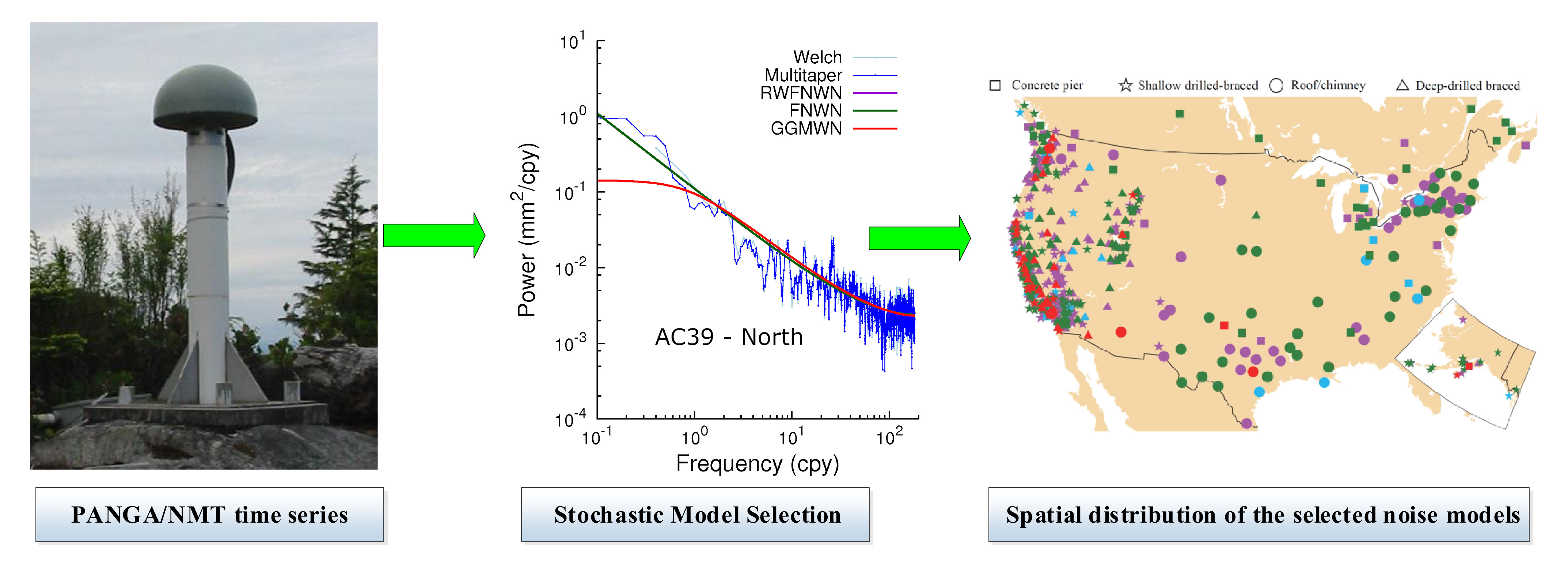
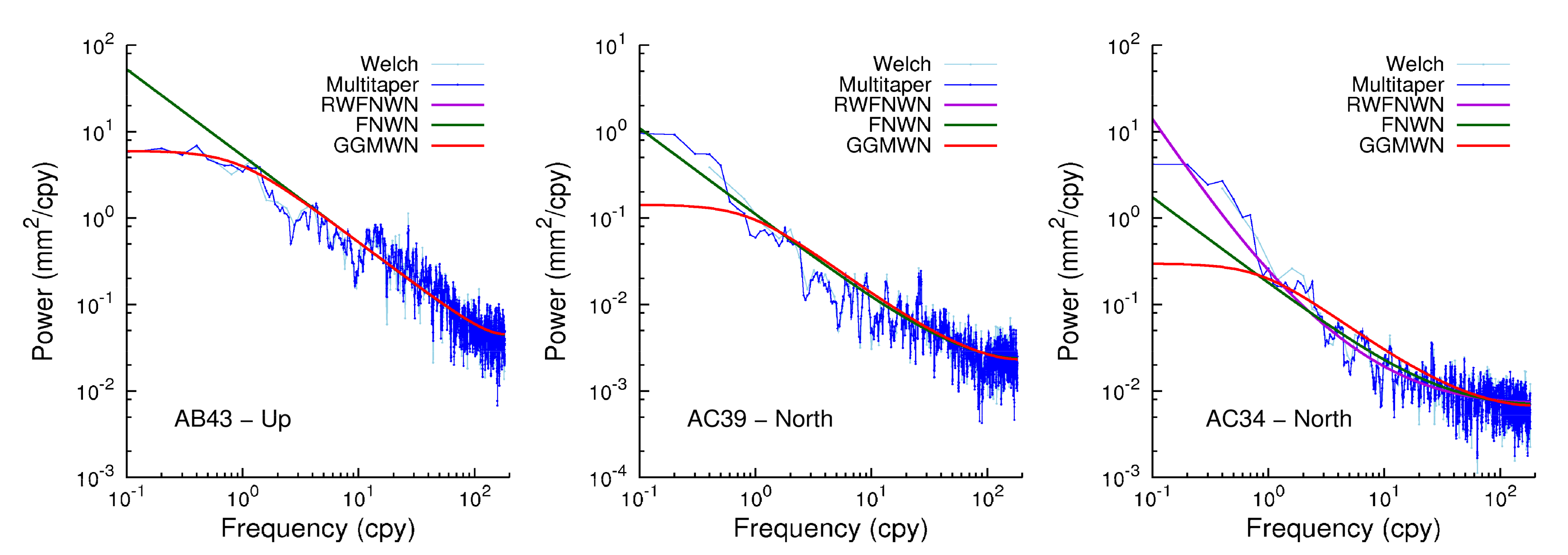
2.3. Stochastic Model Selection Criteria and Simulation Experiment

Power-law noise with a spectral index of −1 is called flicker noise (FN). Random walk (RW) noise has a spectral index of −2. Generalized Gauss Markov (GGM) noise is similar to power-law noise (PL) but flattens below a specified frequency. As noted in the introduction and shown in the following sections, the selection of the correct noise model has a significant influence on the trend uncertainty [21,23,53,54]. The theory of selecting the best model to describe the observation has a long history and many research areas simply use the Akaike or Bayesian Information Criterion [55,56]. However, Langbein (2004) followed a more empirical approach by performing Monte Carlo simulations using synthetic noise, and in this way, determined how much the difference between two log-likelihood values of two competing noise models must be before one can confidently choose one over the other [42]. In the report by Langbein (2004) and Santamaría-Gómez et al. (2011), the default noise model for these simulations, or the null model, was in all cases a random walk plus white noise and it was determined how much the log-likelihood value needed to be higher before one could accept another noise model as being better with 99% confidence [42,57]. The log-likelihood value will be abbreviated as MLE since it is estimated with the maximum likelihood method. Differences between two MLE values are represented as dMLE. The likelihood function represents a probability, although not normalized. Therefore, MLE and dMLE are logarithms of the probabilities and have no units.
We repeated the simulations using 5000 daily time series with a length of 10 years of synthetic random walk + white noise, each with amplitudes of 1 mm/yr0.5 and 0.5 mm, respectively—that is, for 5000 simulations, the dMLE for which there are 50 values greater is identified as the 99% level to reject the null hypothesis. The results are shown in Table 1.
The Bayesian Information Criterion (BIC) and BIC_tp are defined as follows (He et al., 2019) [25]:
B I C = 2 M L E + v ln ( N )
B I C _ t p = 2 M L E + ln ( N 2 π ) v  
where MLE = ln(L), the log-likelihood value; ν is the number of parameters in the noise model; N is the number of observations. The noise model with the lowest BIC value is selected. For 10 years of daily observations, ln(N) = 8.2. Following Langbein (2004) and Santamaría-Gómez et al. (2011) [42,57], we can rewrite the difference in BIC values as a difference in MLE values:
4.1 ( v n v b ) + ( M L E b M L E n ) > 0 ?
where v n and v b are the number of parameters and M L E n and M L E b are the MLE values of the null and new models, respectively. If this criterion is larger than zero, then the new noise model (b) is more likely than the null model (n). RWFN and PL have one more parameter than RW while GGM has two more parameters, resulting in correction values of 4.1 and 8.2. For example, the MLE value for the GGM model needs to be 8.2 higher than that of RW before one can be confident that it is a better representation of the noise. These correction values are similar to the values listed in Table 1. For BIC_tp, the weight factor for each extra parameter in the noise model is 3.2 for time series with a length of 10 years instead of 4.1.
As in He et al. (2019) [25], we only consider the detection of GGM to be the most likely noise model significant if ϕ < 0.98; this parameter is also estimated by Hector. If this condition is not met, then the second most likely noise model is chosen. He et al. (2019) explained that this condition implies that we only detect GGM noise with flattening that already starts around a period of 1 year [25]. For the rest of this research, this extra condition of ϕ < 0.98 was always applied in addition to satisfying Equation (4).
The values of the parameters in the noise models used in the Monte Carlo simulations of Langbein (2004) [42] are slightly different from the noise values discussed here. To ensure the most realistic results, we determined the mean values for each estimated noise model for the horizontal and vertical components for our 5000 time series, see Table 2 and Table 3. For each noise model, 5000 synthetic noise time series were generated. Each of them was analyzed using FN + WN (Flicker Noise + White noise), RW + FN + WN (Random Walk + Flicker Noise + White noise), GGM + WN (Generalized Gauss Markov + White Noise), and PL + WN (Power-law + White noise).
Instead of tabulating the 99% quantile of the difference in M L E b M L E n , we show all differences as box–whisker plots in Figure 2 and Figure 3. Thus, if all values in the box–whisker plots were negative, one could be 100% sure that using the selected noise model (the noise model we think is correct) with the highest MLE value would indeed reflect the true underlying noise models (better than the alternative noise models). One can see that this is not always the case. Applying the BIC correction (BIC and BIC_tp), resulting in the blue box–whisker plots, reduces the MLE of noise models with more parameters than the test/null model and increases it for models with fewer parameters. Therefore, BIC helps to detect FN noise while reducing the rate of detecting GGM noise. The red box–whisker plots represent the results of using BIC_tp. BIC helps increase the number of true positives (the true noise model was selected) and reduce the number of false positives (the false noise model was selected). Overall, its performance is better than BIC; thus, it will be used for the rest of this research.
From Figure 2 and Figure 3, it can be concluded from the RW + FN panels with positive box–whisker plots ( M L E b M L E n > 0 ) that in many cases, PL + WN noise is detected while in fact, the true underlying noise is RW + FN + WN [23]. On the other hand, if RW + FN + WN noise is detected, then we have high confidence that it is correct since false positives are extremely rare—see also He et al. [25]. Important for this research is the fact that for synthetic GGM, the MLE of the other noise models is always lower than that of GGM. In addition, from the other panels of Figure 2 and Figure 3 one can also see that GGM is almost never selected when the underlying noise is not GGM. Thus, we can conclude with great confidence that any detection of GGM using BIC or BIC_tp is correct.
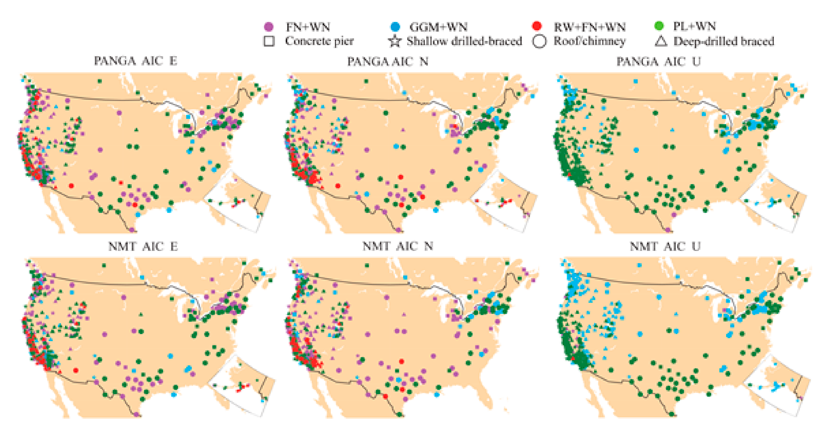
The random walk + flicker + white noise model was used by Langbein and Svarc [40] in the analyses of their time series. However, the analyses of our time series show that some flatten at low frequencies, which can be better described by a GGM noise model. These different conclusions might be caused by the fact that Langbein and Svarc [40] analyzed regionally filtered time series, whereas we are looking at unfiltered time series that are noisier and in which the smaller random walk signal might be hidden.
Note that Santamaría-Gómez et al. (2011) [57] concluded that using neither AIC nor BIC is recommended as a means to discriminate between models. Using similar Monte Carlo simulations, the reader should be convinced that for the time series of a length of 10 years used in this research, the performance of BIC and BIC_tp is actually similar to that of using the approach of Langbein and Svarc (2019) [40], leaving the general debate of using or not using the information criteria in the selection of the stochastic noise model for the future.

3. Results and Discussion with Real GPS Time Series

3.1. Multitaper Analysis

We have previously discussed the selection of noise models based on log-likelihood values. However, we can also illustrate the difference in stochastic properties of the noise by power spectral density (PSD) plots. Here, we used the Welch method to compute the PSD. We further used the multitaper method of Thomson [58], using the software of Prieto [59], which produces increasingly accurate estimates of the power at low frequencies [60]. Figure 4 shows three examples that illustrate the different behavior at low frequencies. For some stations, a flattening of the power spectrum can be observed, while for other stations, the slope of the power spectra increases at low frequencies and is better described by a random walk noise model. For the left and center panels in Figure 4, the RW part of the RW + FN + WN model was very small and resulted in very similar power spectra as FN + WN.

3.2. Episodic Tremors and Slip

In this research, the focus is on the noise within GPS time series. However, the trajectory model should be accurate in order to ensure that the separation between geophysical processes and other noise sources is realistic. This is especially important for stations that experience episodic tremors and slip (ETS) events. ETS events are restricted to 20 stations located specifically in the Cascadia area. Table 4 displays the results of modeling or not the ETS events using 100 days of postseismic decay time scale for the two processing centers, PANGA and NMT. Table A2 and Table A3 in Appendix A provide more details on the stochastic noise models’ behavior of each East North Up (ENU) component. Note that the results using 30, 80, and 130 days of postseismic relaxation are included in the appendices (see Table A4), but do not vary significantly compared with the results shown in Table A4. It is worth emphasizing that there is a slightly higher frequency rate of selecting the RW + FN + WN model, for both PANGA and NMT processing, when including a small postseismic relaxation delay (i.e., 30 or 80 days) in the functional model, which indicates that the remaining relaxation phenomenon is modeled as RW noise.
From Table 4, we can see that there is a much higher chance of selecting an RW component (i.e., the RW + FN + WN model) in the stochastic model for both processing strategies without modeling the ETS. Looking at the results using the BIC_tp, the percentages are 10.00% and 5.00% for PANGA and NMT, respectively, whereas with the ETS model, the percentages decrease to 1.67% and 0.00% for PANGA and NMT, respectively. The results are similar using the AIC. In addition, we can see that the AIC selects slightly more often the RW component in the case of PANGA processing when there is no modeling of the ETS events. This result echoes the conclusions in He et al. (2019) [25]. where it was found that the AIC criteria were slightly more sensitive to the detection of the RW component. Furthermore, with ETS modeling, the proportion of GGM + WN increases, from approximately 37% to 58% and approximately 41% to 51% for the PANGA and NMT solutions, respectively. In addition, modeling the ETS has a significant effect on the selection of the stochastic noise model of the GPS time series, as shown in Table A5 (Appendix A). As an example, the model changes when including or not including the ETS events, which is approximately 35% and 40.0% for PANGA and NMT, respectively, using the AIC, and approximately 21.7% for both PANGA and NMT with the BIC_tp criteria. In particular, for the variation in the stochastic noise models, the GGM + WN model more likely fits the time series of the Up component than the other models for the 20 sites considered here. Table A2 and Table A3 show that the changes in stochastic noise models mainly occurred in the East and North components.

3.3. Spatial Variations Analysis

In this section, we use the 568 stations located in North America and displayed in Figure 5. To process the time series and select the optimal stochastic noise model using the AIC and BIC_tp criteria, we follow the same approach described in the previous sections. Note that for the stations experiencing ETS events in the Cascadia region, the postseismic relaxation was set up to 100 days to be consistent with our results established in the previous section. In addition, we implement automatic offset detection on the GPS residual time series discussed in Fernandes and Bos (2016) [44].
The selected stochastic noise models using AIC and BIC_tp over 568 stations show high consistency (approximately 98.7% and 98.6% for the PANGA and NMT solutions, respectively). The significant differences in the selection of the stochastic noise model between AIC and BIC_tp applied to the PANGA and NMT solutions are displayed in Table 5. We can see that AIC is generally more sensitive to RW noise in the selection of the RW + FN + WN and GGM + WN models, which supports the previous conclusions mentioned in He et al. (2019) [25]. Table 6 shows the percentage of stochastic noise models selected over the 568 stations for the PANGA and NMT solutions with only the AIC (for ENU and the average of the 3 components). The difference in terms of percentage is much higher in the Up component, where, for the NMT solutions, the GGM + WN model is more likely selected, and the PL + WN for the PANGA time series.
The results in Table 6 also emphasize that the RW + FN + WN is approximately 8–14% for the horizontal components and only approximately 0.2% for the Up component; this is also demonstrated in Figure 5. Spatial distribution of the selected noise models using AIC (there is slight difference with BIC_tp—the main difference is that AIC is a little more sensitive to the RW noise, as shown in Table 5). The RW + FN + WN noise is much less in the Up component. In fact, we can see that all four models are selected in the horizontal components, whereas the vertical components have mostly PL + WN and GGM + WN noise models. This result holds in the analysis of the time series of both processing centers. This difference can be attributed to the fact that the vertical component is generally much noisier (~3 times greater) than the East and North components [22]. He et al. (2019) [25] concluded that GGM + WN fits slightly better than the other noise models for the vertical component, which is also supported by our results.
To further analyze the potential correlation of sites showing RW noise with geophysical phenomena, we highlight the sites for both NMT and PANGA solutions in Figure 5 (i.e., red dot for the RW + FN + WN). Most are located near the coasts (distance <10 km from the shoreline—see Figure A1 in Appendix A, which shows the spatial distribution of the RW sites for both PANGA/NMT) and in known tectonically active areas: the Cascadia subduction zone and San Andreas strike-slip fault. This result is in agreement with our results shown in the previous section, where we demonstrated that when the functional model does not completely capture all geophysical signals (due to earthquakes and/or postseismic deformation and possibly generates short-duration transient signals), the algorithm estimates higher amplitude RW noise than in much less tectonically active areas. The results also show that the detected RW amplitudes are larger than 0.5   m m / y r 0 . 5 . (see Figure A1 and Table A6 in Appendix A).

3.4. Relation between Type of Noise and Type of Monument

First, we analyze the velocity uncertainty of the 568 GPS stations related to type of monument. Figure 6 shows the spatial distribution of the velocity uncertainty with the optimal stochastic noise model, using AIC, for PANGA and NMT. From Figure 6, we can see that the Nevada/Idaho and Utah regions are quieter (i.e., lower uncertainty value) than the other areas, especially for the NMT solutions. In contrast, the Washington/Oregon region is noisier (i.e., higher uncertainty value). It can also be observed that there is no obvious pattern between types of monuments and velocity uncertainty. DDB monuments have the largest percentage of random walk component according to Figure 6. These monuments are mostly located along the San Andreas fault in central and southern California. Therefore, they display larger noise amplitudes due to high tectonic activities [61,62,63]. CP monuments are mostly located near Washington/Oregon states and near the Great Lakes. To recall the previous discussion, the Pacific Northwest is also a tectonic active area with the Cascadia subduction zone [64]. The Great Lakes region is not a strong tectonic active area but is known for strong postglacial rebound [65] and complex geodynamics [66]. Besides, there are other geodynamic mechanisms related to the lakes such as the lake-level variability impacted by climate change [67]. For this type of monument, GGM + WN is often the optimal model.
Furthermore, the statistical analysis of Table A7 and Table A8 together with Figure 7 show that there is diversity in the results depending on the types of monuments and components. Previous results established that the FN + WN model is the stochastic noise model mostly selected for East and North components. Our results support that the FN + WN and PL + WN are still the most common noise models, but in the up component, GGM + WN is more present as well for both PANGA and NMT solutions.
Note that the largest ratio of GGM + WN model mainly appears for the CP monuments (44.4% Up (PANGA) and 60% Up (NMT)). Thus, we cannot conclude on the discrimination between type of monuments and stochastic noise model. The noise properties are spatially varying so we cannot define a general ‘preferred’ noise model for a type of monument since it depends on the geographical distribution of the monument. The largest ratio of RW mainly appears in DDB and SDB monuments. Moreover, the largest percentage of RW component is prominent in the SDB and DDB types of monuments.
From Table A7 and Table A8, we can see some slight variations when comparing the results between the East and North components for each type of monument. The percentage of the selected RW + FN + WN model is the largest for the DDB monuments on the East component (~12.15% PANGA; 11.6% NMT), but not on the North component (~11.60% PANGA; 12.15% NMT). Instead, the probability of selecting this noise model is the largest for the SDB monuments on the North component (~19.10% PANGA; 16.73% NMT).
This sensitivity to RW noise is not experienced for the CP and RTC monuments. However, one needs to take into account that in our study, most of the CP monuments are installed in tectonically active areas where higher noise amplitude can mask the RW component. The RW component models the small-amplitude, short-duration, transient signals originating from regional (or local) deformations, which seem to be more present in the time series of the SDB and DDB monuments.
In addition, the stochastic noise properties of the vertical component are mostly modeled with PL + WN. However, the GGM + WN model challenges this result in the case of CPs where the percentage is higher, approximately 44.44% and 60.00% for PANGA and NMT solutions, respectively. Thus, these time series of the vertical component experience flattening at a low frequency, as discovered and analyzed by He et al. (2019) [25].
To further support this result, we draw a boxplot of the velocity uncertainties with the selected FL + WN and optimal noise model, as shown in Figure 8 and Figure 9, respectively. In Figure 8, a clear trend is seen from stable monuments such as the DDBm. However, Figure 9 does not show the differences between the types of monuments. We think that a large number of receivers on CP experience GGM noise, which halves the trend uncertainty. The total effect is a reduction in the correlation between the type of monument and velocity uncertainties.
From Figure 8 and Figure 9, we can also see that the RTC monument performs as well as the DDBm. To understand this result, we should look again at Table A7 and Table A8 in the Appendix A; they display the amplitude of the white noise for the PANGA processing using the AIC criteria. We notice that the amplitude of the white noise is largest for the RTC monuments. Therefore, the RTC setup may partially mask small, transient, geophysical signals by increasing the amplitude of the white noise, rendering this setup disadvantageous for geophysical studies at the regional scale when looking at small amplitude short-duration signals. From Table A7 and Table A8, we can also see that the estimated white noise amplitude is very different between the NMT and PANGA solutions. As discussed in Section 1, PANGA uses GIPSY–OASIS (GIPSYX) without any scale parameter in the Helmert transform, whereas the NMT solution results from the processing with GAMIT/GLOBK including a scale parameter. It results in different stochastic noise properties of the time series, with a smaller scatter than the PANGA ones (~30%), and hence, a smaller noise amplitude.
In light of this discussion, we can conclude that the higher white noise amplitude associated with the RTC monuments can mask the presence of a RW component (see Table A9 and Table A10 in Appendix A, which show the relation between the monument type and estimated noise model) in the stochastic noise model than in other monuments (SDBm and DDBm). This can explain why the velocity uncertainties in Figure 8 and Figure 9 are smaller.
From the above results and analysis, we can conclude that there is reduced discrimination as to which monument performs the best over the three coordinates. The spatial distribution of the monuments supersedes the type of monuments in the selection of the noise model for the global, not regionally filtered, GNSS time series. Previous studies, such as Herring et al. (2016) [34], have warned about the spatial distribution across North America. Williams et al. (2004) restricted their study to a small area to determine the influence of the various types of monuments [22]. Beavan (2005) [68] concluded that monument noise is not the dominant factor in the stochastic noise properties of the GPS time series; hence, we corroborate his results. Finally, we supplement CME reduction and the elimination of some stations in active areas in the Appendix A, to explore the effect of regional filtering and large postseismic relaxation events on monument performance. We can see that regional filtering does not change the overall results. The DDBm is still the best monument type, which supports what we have already previously discussed in this paper.

4. Conclusions

This work has investigated the noise properties of 568 GPS daily position time series with a length of 10 years in North America, computed by NMT and PANGA, together with their spatial distribution. These time series are given with respect to a global reference frame (ITRF2008) and no regional filter has been applied.
To model the noise in the GPS time series, the following models were used: FN + WN, RW + FN + WN, GGM + WN, and PL + WN. The selection of the optimal noise model was based on the log-likelihood value and the information criteria (i.e., AIC, BIC, BIC_tp) to avoid overselecting noise models with many parameters. This approach was criticized by authors of various studies who do not recommend the use of AIC or BIC. However, when we apply these information criteria to Monte Carlo simulations of synthetic time series, we can demonstrate that for noise RW + FN + WN, we have a very low percentage of false positives. Thus, if we detect RW + FN + WN noise, then we have high confidence this is correct. On the other hand, we still have a high number of false negatives, which means that PL + WN is still detected, while in reality, the underlying noise model is RW + FN + WN, in agreement with previous studies [23,25]. The simulations also demonstrate that we are able to reliably detect the GGM noise model. Statistically, we found that for around 10% of the stations, the power spectral density shows flattening at low frequencies, which can be better described with a Generalized Gauss Markov (GGM) noise model, further extending the conclusions of He et al. (2019).
For the Cascadia subduction region, which is tectonically active, it is necessary to include episodic tremor and slip in the trajectory model. Otherwise, the misfit between observations and model is absorbed as a large random walk component, which affects the value of the estimated linear motion and increases its uncertainty. In addition, our results show that the selection of the RW component in the RW + FN + WN model accounts for a non-negligible percentage when not modeling the ETS events, whereas when properly modeled, the GGM + WN and PL + WN models are more often selected. Note that AIC is generally more sensitive to the RW noise in the selection of the RW + FN + WN and GGM + WN model.
Furthermore, the spatial distribution of selected noise models shows a pattern in our case study. Stations including the RW component are generally located near the coasts (distance <10 km from the shoreline) or in active tectonic areas (Cascadia subduction zone, San Andreas fault). In terms of differences between the two processing strategies, the time series from the NMT solutions are more often modeled with the GGM + WN than the PANGA solution, therefore exhibiting a flattening of the power-spectrum. In addition, the largest percentage of RW + FN + WN model is selected in SDB and DDB monuments mainly for the horizontal components. The PL + WN and FN + WN models are generally the dominant stochastic noise models for the monuments, but the GGM + WN is also often selected for the CP monuments, especially on the Up component, which means that the very long time series generated from monitoring the CP monuments are experiencing this flattening at low frequency. The difference in results between AIC and BIC_tp is relatively small for each monument in selecting the various stochastic noise models. However, we show that the amplitude of the white noise is largest for the RTC. Therefore, the RTC setup may partially mask small transient geophysical signals by mismodeling the amplitude of the noise. Moreover, when investigating the relationship between the various types of monuments and the estimation of the geophysical signals, the results emphasized that the smallest uncertainties associated with the tectonic rate are recorded by the DDBm monuments for the East and North components, especially selecting the FL + WN model. On the vertical component, the results difference between the DDBm and SDBm is not significant. Additional results obtained by removing CME and monuments located in tectonically active areas (such as the Cascadia subduction zone) show that the uncertainties decrease, especially with CP and DDBm monuments on the East and North components. CP and DDBm monuments are mostly located in tectonically active areas or close to the coastline. Overall, we recommend the use of DDBm in noisy or tectonically active areas. However, their stochastic noise properties are different to those in more stable areas. Therefore, we conclude that the location of the station supersedes these types of monuments in the estimation of the tectonic rate uncertainty, supporting previous studies [34,68].

Author Contributions

X.H., M.S.B. and J.-P.M. writing-original draft preparation and methodology; R.F. and T.M. reviewed and edited the manuscript. T.M. provided some of the resources displayed in this study; W.J. and W.L. made the common mode error filtering analysis. All authors have read and agreed to the published version of the manuscript.

Funding

Xiaoxing He was sponsored by National Natural Science Foundation of China (42104023, 42061077) and Jiangxi University of Science and Technology High-level Talent Research Startup Project (205200100564). Machiel Bos and Rui Fernandes were sponsored by national Portuguese funds through FCT in the scope of the project UIDB/50019/2021—Instituto Dom Luiz. Computational resources were provided by C4G-Collaboratory for Geosciences (PINFRA/22151/2016).

Institutional Review Board Statement

Not applicable.

Informed Consent Statement

Not applicable.

Data Availability Statement

The processed time series are available at ftp://data-out.unavco.org/pub/products/position/.

Acknowledgments

We thank Thomas Herring and Mike Floyd of MIT for their helpful discussion on PANGA and NMT solution.

Conflicts of Interest

The authors declare no conflict of interest.

Appendix A

Table A1. Statistics of data gap over the 568 sites used in this study.
Data GapPANGAPANGAPANGANMTNMTNMT
ENUENU
<3%93.7%93.5%97.0%91.7%92.6%97.9%
Mean1.17%1.09%0.84%1.24%1.18%0.81%
Max7.91%6.41%7.61%6.79%7.07%7.20%
Min0.05%0.05%0.05%0.05%0.05%0.05%
Table A2. Stochastic noise model behavior of ENU component for the 20 GPS stations selected in the Cascadia area (PANGA).
ENUModelNo-ETSETS
AICBICtpAICBICtp
ERW + FN + WN20.00%15.00%10.00%5.00%
FN + WN30.00%60.00%30.00%45.00%
GGM + WN0.00%0.00%20.00%20.00%
PL + WN50.00%25.00%40.00%30.00%
NRW + FN + WN15.00%15.00%0.00%0.00%
FN + WN20.00%40.00%15.00%25.00%
GGM + WN30.00%25.00%65.00%65.00%
PL + WN35.00%20.00%20.00%10.00%
URW + FN + WN0.00%0.00%0.00%0.00%
FN + WN0.00%5.00%0.00%0.00%
GGM + WN85.00%85.00%90.00%90.00%
PL + WN15.00%10.00%10.00%10.00%
Table A3. Stochastic noise model behavior of ENU component for the 20 GPS stations selected in the Cascadia area (NMT).
ENUModelNo-ETSETS
AICBICtpAICBICtp
ERW + FN + WN20.00%15.00%0.00%0.00%
FN + WN45.00%65.00%40.00%50.00%
GGM + WN5.00%5.00%40.00%30.00%
PL + WN30.00%15.00%20.00%20.00%
NRW + FN + WN0.00%0.00%0.00%0.00%
FN + WN40.00%60.00%30.00%45.00%
GGM + WN25.00%20.00%30.00%15.00%
PL + WN35.00%20.00%40.00%40.00%
URW + FN + WN0.00%0.00%0.00%0.00%
FN + WN0.00%0.00%0.00%0.00%
GGM + WN95.00%95.00%95.00%95.00%
PL + WN5.00%5.00%5.00%5.00%
Table A4. Selected stochastic noise model with the AIC with varying postseismic relaxation time.
Postseismic Relaxation Time in Days (×10)PANGA-AICNMT-AIC
381013381013
RW + FN + WN42220000
FN + WN10109915141413
GGM + WN3233353530313132
PL + WN1415141415151515
Table A5. ETS effect on the selection of the stochastic noise.
Stochastic Noise Vartion
AICBICtp
PANGA35.00%40.00%
NMT21.67%21.67%
Table A6. The amplitudes (mm) of the RW component of the sites in Figure A1.
SiteENUPANGANMTSiteENUPANGANMTSiteENUPANGANMT
AC15N1.3 1.2 P170E1.2 2.0 P527E1.8 1.3
AC34E1.3 1.5 P197N1.6 1.2 P530N1.2 1.2
AC67N2.0 1.3 P197E1.4 1.5 P530E0.8 0.7
AC67E0.9 1.1 P218N1.8 2.4 P533N0.7 0.5
AV12N1.8 1.7 P238N1.7 1.6 P544E1.0 0.8
AZGBE1.3 1.3 P238E2.8 2.6 P556E0.7 0.8
BBDMN1.7 1.5 P242N2.1 2.3 P563N1.2 1.1
BBDME1.9 2.2 P247N1.1 1.2 P563E1.2 1.1
BEMTN0.6 0.6 P254N1.2 1.3 P568E0.6 0.5
BKAPN0.6 0.6 P254E0.9 0.6 P576N2.1 2.2
BKMSN1.8 1.8 P278N1.2 1.5 P576E3.2 2.4
BKMSE0.7 1.6 P278E1.6 1.6 P585N0.8 0.8
CARHN1.2 1.0 P284N1.2 1.3 P601N0.7 0.6
CARHE1.5 1.5 P284E1.6 1.9 P607N0.8 0.7
CLARN1.0 1.3 P300N2.1 1.7 P610N0.7 0.5
CLARE0.9 0.5 P300E3.1 3.1 P623N0.7 0.6
COPRN0.8 0.8 P302N1.1 1.2 P627N0.7 0.9
CPXXE1.5 1.7 P302E2.7 2.7 P643N1.5 1.5
CSDHE1.4 0.9 P309E1.7 1.4 P649N0.7 0.8
CTMSN0.7 0.6 P317N0.6 0.5 P649E0.7 0.7
CVHSE2.1 1.7 P317E1.5 1.1 P716N1.8 1.3
FMTPN1.2 1.4 P319N0.9 0.7 P716E2.5 2.1
FMVTN1.0 0.9 P376N0.9 1.4 P729N1.6 1.7
GVRSE1.0 0.7 P376E1.1 0.7 P729E2.6 2.3
KBRCE1.8 1.6 P406N2.5 2.3 SELDN2.0 1.4
LBC2N2.1 1.8 P421E2.1 2.4 SELDE0.9 0.8
LBC2E1.5 1.7 P457E0.8 1.0 TOSTN1.1 1.2
LDESN0.6 0.6 P465E1.4 1.3 TXTAN2.3 2.3
OKDTN1.1 1.0 P473E1.1 0.9 VNCON1.4 1.2
OPBLN0.5 0.6 P491N0.8 0.7 VNCOE0.9 0.8
P003E0.9 0.9 P504N0.7 0.6 WCHSN0.9 1.2
P124N1.2 0.9 P511N0.8 0.6 WCHSE1.6 1.2
P125E0.8 0.9 P526N0.8 0.7 WHC1E0.6 0.8
P169E0.5 0.5 P526E1.4 1.0 WNRAN1.3 1.1
P170N1.5 1.4 P527N1.4 1.3 WNRAE0.8 0.8
Table A7. Amplitude (mm) of white noise vs. type of monument (PANGA).
PANGAENU
μσμσμσ
RTC0.660.350.750.320.61.46
CP0.470.350.740.320.250.82
DDB0.660.220.720.320.551.19
SDB0.670.270.750.340.711.27
Table A8. Amplitude (mm) of white noise vs. type of monument (NMT).
NMTENU
μσμσμσ
RTC0.620.310.530.270.290.76
concrete0.550.400.560.260.270.76
DDB0.580.180.530.190.160.55
SDB0.590.200.550.250.150.51
Table A9. Monument type vs. noise model PANGA (AIC).
ENUMonument TypeRW + FN + WNFN + WNGGM + WNPL + WN
EConcrete pier4.44%28.89%11.11%55.56%
Deep-drilled braced12.15%49.72%5.52%32.60%
Roof/chimney5.06%44.30%7.59%43.04%
Shallow-drilled braced8.75%46.77%6.46%38.02%
NConcrete pier4.44%44.44%22.22%28.89%
Deep-drilled braced11.60%47.51%11.05%29.83%
Roof/chimney6.33%26.58%12.66%54.43%
Shallow-drilled braced19.01%39.54%6.84%34.60%
UConcrete pier0.00%0.00%44.44%55.56%
Deep-drilled braced0.55%2.76%8.29%88.40%
Roof/chimney0.00%3.80%21.52%74.68%
Shallow-drilled braced0.00%3.80%13.69%82.51%
Table A10. Monument type vs. noise model NMT.
ENUMonument TypeRW + FN + WNFN + WNGGM + WNPL + WN
EConcrete pier2.22%31.11%15.56%51.11%
Deep-drilled braced11.60%43.09%6.08%39.23%
Roof/chimney2.53%46.84%6.33%44.30%
Shallow-drilled braced9.51%39.54%9.51%41.44%
NConcrete pier2.22%51.11%20.00%26.67%
Deep-drilled braced12.15%45.86%6.63%35.36%
Roof/chimney3.80%39.24%15.19%41.77%
Shallow-drilled braced16.73%44.87%6.84%31.56%
UConcrete pier0.00%4.44%60.00%35.56%
Deep-drilled braced0.55%4.97%33.15%61.33%
Roof/chimney0.00%0.00%27.85%72.15%
Shallow-drilled braced0.00%2.66%32.32%65.02%
Figure A1. Spatial distribution of the RW sites for PANGA/NMT (the rectangular area in the lower left corner of the figure is a zoom view of all the stations under P406 without station name mark).
Remotesensing 13 04534 g0a1
As mentioned in the previous section on ‘GPS processing’, the PANGA and NMT solutions did not implement any regional filtering. We extract the regional common mode error (CME) on the GPS network for both PANGA and NMT solution. For filtering on the CME, we implement the VBPCA method to extract CME (Li et al., 2020). The VBPCA method imposed a priori distributions on the model parameters and estimated the hyperparameters by maximizing the evidence of observed signals. This method can naturally handle missing data in the Bayesian framework and utilizes the variational expectation–maximization iterative algorithm to search the CME for the incomplete GNSS position time series. Moreover, it can automatically select the optimal number of principal components for data reconstruction and be more reliable against the overfitting problem than other statistical signal decomposition methods. The boxplots with CME filter of the velocity uncertainties with the selected FL + WN and optimal noise model are shown in Figure A2aa. From Figure A2aa together with Figure 8 and Figure 9, we can see that regional filtering does not change the overall results. The DDBm is still the best monument type. The CME removal is only interesting looking at the CP monuments. However, we only have 45 CP in this study. In addition, some of the 568 analyzed sites were located in a region that was known to contain tectonic or volcanic transient events, which will affect the stochastic noise properties and, therefore, the monument performance. Thus, we removed these sites (reducing the total number to 538 sites). The boxplot figures after filtering the CME and with optimal model selection are shown in Figure A2bb. Overall, the filter improves only the results with CP monuments. These monuments are located in the Pacific Northwest, with postseismic relaxation, and this result supports what we have already said in this study.
Figure A2. Boxplot with CME filter with FN + WN model for PANGA (P.) and NMT (N.) solution. (a) Boxplot with CME filter with FN + WN model for PANGA (P.) and NMT (N.). (b) Boxplot with CME filter with FN + WN model for PANGA and NMT (large postseismic relaxation sites removed).
Remotesensing 13 04534 g0a2
Figure A3. Boxplot with CME filter with optimal model for PANGA and NMT solution. (a) Boxplot with CME filter with optimal model for PANGA and NMT. (b) Boxplot with CME filter with optimal model for PANGA and NMT (remove large postseismic relaxation sites).
Remotesensing 13 04534 g0a3

Appendix B

For the postseismic relaxation or Episodic Tremor and Slip events, we assume that the observations are the sum of a deterministic model and stochastic noise. This deterministic model is as follows:
X = i = 0 n P p i ( t t R ) i + i = 1 n J b j H ( t t j ) + i = 1 n F s i sin ( ω i t ) + c i cos ( ω i t ) + i = 1 n T e i ( 1 exp ( ( t t i ) / T i ) ) + j = 1 n L a j log ( 1 + ( t t j ) / T j ) ) + k = 1 n T u k 2 [ tanh ( ( t t k ) / T k ) ) 1 ] l = 1 n L a l × f l ( t )
where p i are the coefficients of a n p degree polynomial. By default, n p = 1 means a linear trend. H ( t ) is the Heaviside step function and used to model offsets with amplitudes b j . An annual and semiannual signal are commonly included in the model and therefore have their own keywords, ’seasonal’ and ’halfseasonal’, in Hector [43]. In the equation, their angular velocities are represented by ω i . Other periodic signals need to be entered using the keyword ’PeriodicSignals’, followed by a list of their periods in days. The time of the slow slip event and the delay of the postseismic deformation are required as input parameters for the estimation of the ETS using Hector with a hyperbolic tangent by providing two parameters, t k and T k .

Appendix C

Table A11. Monument types of the analyzed 568 sites: concrete pier (CP), Deep-drilled brace (DDB), Shallow-drilled brace (SDB), and Roof top/Chimney (RTC).
SiteTypeSiteTypeSiteTypeSiteTypeSiteTypeSiteTypeSiteTypeSiteType
1NSURTCCORVSDBMAT2SDBP114DDBP256DDBP420DDBP557DDBROCKSDB
AB07SDBCOVGRTCMHCBRTCP115DDBP257SDBP421DDBP558DDBSASKCP
AB22SDBCPXXSDBMICWCPP116DDBP258SDBP422DDBP563DDBSCIASDB
AB43SDBCRBTSDBMIDADDBP117DDBP259DDBP423DDBP566SDBSDHLSDB
AB44SDBCRU1SDBMIDSCPP118SDBP262DDBP427DDBP568SDBSEATRTC
AC15DDBCSCISDBMIG1SDBP119SDBP267DDBP429DDBP569SDBSEDRDDB
AC20SDBCSDHSDBMIHOCPP121DDBP268DDBP432DDBP570SDBSELDCP
AC27SDBCSSTSDBMIIRCPP124DDBP272DDBP436DDBP572DDBSHE2CP
AC31SDBCTBRRTCMLFPSDBP125DDBP273SDBP437DDBP576SDBSHINDDB
AC34SDBCTDMSDBMNMCSDBP128DDBP274SDBP439DDBP579DDBSHLDDDB
AC39SDBCTGURTCMOILDDBP132DDBP275DDBP442DDBP580SDBSHOSDDB
AC41SDBCTMSSDBMPLECPP134SDBP276DDBP445SDBP581DDBSHRVRTC
AC59SDBCTPURTCMPWDSDBP138DDBP278SDBP448SDBP583SDBSIBYCP
AC63SDBCVHSSDBMSOLCPP139SDBP280DDBP449SDBP585SDBSMELDDB
AC67SDBDDSNSDBMTFVRTCP141SDBP283DDBP451DDBP592DDBSNFDRTC
ADRICPDOBSCPNANOCPP148SDBP284SDBP457SDBP593SDBSPICDDB
AGMTSDBDRAOCPNCPORTCP154SDBP285DDBP460DDBP595SDBSPK1RTC
AHIDSDBDSSCSDBNCSWRTCP156DDBP287SDBP461DDBP599SDBSPMSSDB
AL30RTCDUBOCPNEAHCPP157SDBP288SDBP462SDBP601SDBSTJOCP
AL50CPDVPBSDBNEDRRTCP160DDBP289SDBP463SDBP606SDBSVINSDB
AL60RTCECFSSDBNEGIRTCP163DDBP290SDBP465DDBP607SDBTABLSDB
ALBHCPECSDDDBNHRGSDBP164SDBP293SDBP466DDBP610SDBTBLPSDB
ALGOCPELIZSDBNHUNRTCP165DDBP294DDBP467SDBP611SDBTHCPSDB
ALPPSDBESCUCPNJTWRTCP166SDBP295SDBP468DDBP615SDBTHU3CP
ARCMRTCEWPPSDBNMRORTCP167SDBP296SDBP469SDBP616DDBTOIYDDB
ARPGRTCFERNDDBNMSFRTCP168SDBP297SDBP471DDBP617SDBTONODDB
AV01SDBFGSTSDBNOR3CPP169SDBP300DDBP472DDBP618SDBTORPSDB
AV02SDBFMTPSDBNYBHRTCP170SDBP301DDBP473SDBP621SDBTOSTSDB
AV06SDBFMVTSDBNYBTRTCP171SDBP302DDBP474DDBP622SDBTPW2SDB
AV07SDBFOOTDDBNYCLRTCP174SDBP305DDBP476SDBP623DDBTWHLSDB
AV08SDBFORESDBNYCPRTCP175DDBP306DDBP478SDBP626SDBTXABRTC
AV09SDBFRDNCPNYDVRTCP178SDBP309DDBP480DDBP627SDBTXAMRTC
AV10SDBFREDDDBNYFDRTCP180SDBP312DDBP482DDBP636DDBTXCHCP
AV11SDBGAATRTCNYFSRTCP182DDBP313DDBP483DDBP643SDBTXCOCP
AV12SDBGARFRTCNYFVRTCP183SDBP314SDBP484SDBP649DDBTXDRRTC
AV16SDBGARLDDBNYHCRTCP185SDBP315DDBP485SDBP651DDBTXELRTC
AV18SDBGOBSSDBNYHSRTCP186DDBP316DDBP486DDBP653SDBTXHERTC
AZGBRTCGODECPNYLVRTCP187SDBP317SDBP490SDBP674DDBTXLFRTC
BAIECPGOSHDDBNYMDRTCP188SDBP318DDBP491SDBP675SDBTXLLRTC
BAMFSDBGVRSSDBNYMLRTCP189SDBP319DDBP504SDBP677DDBTXPERTC
BAR1SDBHAMPRTCNYONRTCP192DDBP324SDBP511DDBP678DDBTXPRRTC
BAYRCPHCMNSDBNYPDRTCP196DDBP326SDBP513SDBP683DDBTXSARTC
BBDMSDBHLFXCPNYPFRTCP197SDBP332SDBP514DDBP684SDBTXSNRTC
BBIDSDBHOGSCPNYSTRTCP206DDBP341SDBP515DDBP698SDBTXSTRTC
BBRYSDBHUNTSDBNYWLRTCP208SDBP344DDBP516DDBP700SDBTXTARTC
BCOVSDBHVYSSDBNYWTRTCP210DDBP354SDBP519DDBP706DDBTXTYRTC
BEMTSDBHWUTCPOHASRTCP211DDBP356SDBP523DDBP710SDBTXVARTC
BEPKSDBIDDRCPOKDTRTCP212DDBP367DDBP525SDBP716SDBTXWARTC
BILLDDBKBRCSDBOPBLSDBP213DDBP370SDBP526SDBP720SDBTXWFCP
BKAPSDBKNGSRTCOPCLSDBP215DDBP371SDBP527DDBP726DDBUCLUCP
BKMSSDBKNTNCPORMTSDBP216DDBP372DDBP528DDBP727SDBUNIVCP
BLW2CPKOKBRTCOVLSSDBP218DDBP374DDBP529DDBP729DDBUSLOSDB
BLYTSDBKTBWSDBOXYCSDBP227SDBP376DDBP530DDBP741RTCVALDCP
BMHLSDBKYBORTCP002DDBP228SDBP377DDBP531DDBP742RTCVCAPRTC
BREWCPKYVWSDBP003DDBP230SDBP387DDBP532DDBPARYRTCVDCYSDB
BRPKSDBLACRDDBP091SDBP231SDBP388DDBP533DDBPCOLRTCVIMTSDB
BSMKRTCLANDDDBP092SDBP232DDBP394DDBP535DDBPGC5CPVNCOSDB
BSRYSDBLANSCPP093SDBP233DDBP395DDBP536DDBPSDMSDBVNCXSDB
BTDMSDBLBC2SDBP094SDBP234DDBP397SDBP537DDBPTALSDBVNPSSDB
BURNSDBLDESSDBP095DDBP237SDBP398DDBP538DDBPVE3CPVTISSDB
CABLSDBLDSWSDBP099SDBP238DDBP401DDBP540DDBPVRSSDBWCHSSDB
CANDDDBLEBACPP100DDBP241SDBP402DDBP543DDBPWELSDBWHC1RTC
CARHSDBLEWIDDBP102SDBP242DDBP404DDBP544DDBQCY2DDBWIDCSDB
CASTDDBLFRSSDBP104DDBP243SDBP406DDBP546DDBQUADSDBWMAPSDB
CDMTSDBLINHRTCP106DDBP244SDBP408DDBP547DDBRAMTSDBWNRASDB
CEDADDBLKCPSDBP108SDBP247SDBP409DDBP549DDBRCA2SDBWOMTSDB
CHWKSDBLL01SDBP109DDBP250SDBP411DDBP550DDBREDMSDBWRHSSDB
CIRXSDBLMCNRTCP110SDBP252DDBP412DDBP551DDBRG07SDBWVRARTC
CJMSSDBLORSSDBP111SDBP253SDBP414DDBP553DDBRG09SDBYBHBCP
CLARSDBLOWSSDBP112SDBP254SDBP417DDBP554DDBRHCLSDBZAB1RTC
COPRSDBMASWSDBP113DDBP255DDBP418DDBP556DDBRNCHSDBZDV1RTC

References

  1. Segall, P.; Davis, J.L. GPS applications for geodynamics and earthquake studies. Annu. Rev. Earth Planet. Sci. 1997, 25, 301–336. [Google Scholar] [CrossRef] [Green Version]
  2. Fernandes, R.M.S.; Ambrosius, B.A.C.; Noomen, R.; Bastos, L.; Combrinck, L.; Miranda, J.M.; Spakman, W. Angular velocities of Nubia and Somalia from continuous GPS data: Implications on present-day relative kinematics. Earth Planet. Sci. Lett. 2004, 222, 197–208. [Google Scholar] [CrossRef]
  3. Fernandes, R.M.S.; Bastos, L.; Miranda, J.M.; Lourenço, N.; Ambrosius, B.A.C.; Noomen, R.; Simons, W. Defining the plate boundaries in the Azores region. J. Volcanol. Geotherm. Res. 2006, 156, 1–9. [Google Scholar] [CrossRef]
  4. Bock, Y.; Melgar, D. Physical applications of GPS geodesy: A review. Rep. Prog. Phys. 2016, 79, 106801. [Google Scholar] [CrossRef] [PubMed]
  5. Montillet, J.P.; Williams, S.D.P.; Koulali, A.; McClusky, S.C. Estimation of offsets in GPS time-series and application to the detection of earthquake deformation in the far-field. Geophys. J. Int. 2015, 200, 1207–1221. [Google Scholar] [CrossRef] [Green Version]
  6. Amiri-Simkooei, A.R.; Hosseini-Asl, M.; Asgari, J.; Zangeneh-Nejad, F. Offset detection in GPS position time series using multivariate analysis. GPS Solut. 2019, 23, 13. [Google Scholar] [CrossRef]
  7. Sauber, J.; Plafker, G.; Molnia, B.F.; Bryant, M.A. Crustal deformation associated with glacial fluctuations in the eastern Chugach Mountains, Alaska. J. Geophys. Res. Solid Earth 2000, 105, 8055–8077. [Google Scholar] [CrossRef] [Green Version]
  8. Tregoning, P.; Watson, C.; Ramillien, G.; McQueen, H.; Zhang, J. Detecting hydrologic deformation using GRACE and GPS. Geophys. Res. Lett. 2009, 36. [Google Scholar] [CrossRef] [Green Version]
  9. Husson, L.; Bodin, T.; Spada, G.; Choblet, G.; Kreemer, C. Bayesian surface reconstruction of geodetic uplift rates: Mapping the global fingerprint of Glacial Isostatic Adjustment. J. Geodyn. 2018, 122, 25–40. [Google Scholar] [CrossRef]
  10. Turner, R.J.; Reading, A.M.; King, M.A. Separation of tectonic and local components of horizontal GPS station velocities: A case study for glacial isostatic adjustment in East Antarctica. Geophys. J. Int. 2020, 222, 1555–1569. [Google Scholar] [CrossRef]
  11. King, M.A.; Penna, N.T.; Clarke, P.J.; King, E.C. Validation of ocean tide models around Antarctica using onshore GPS and gravity data. J. Geophys. Res. 2005, 110, B08401. [Google Scholar] [CrossRef] [Green Version]
  12. Thomas, I.D.; King, M.A.; Clarke, P.J. A comparison of GPS, VLBI and model estimates of ocean tide loading displacements. J. Geodesy 2007, 81, 359–368. [Google Scholar] [CrossRef] [Green Version]
  13. Penna, N.T.; Bos, M.S.; Baker, T.F.; Scherneck, H.G. Assessing the accuracy of predicted ocean tide loading displacement values. J. Geodesy 2008, 82, 893–907. [Google Scholar] [CrossRef] [Green Version]
  14. Penna, N.T.; Clarke, P.J.; Bos, M.S.; Baker, T.F. Ocean tide loading displacements in western Europe: 1. Validation of kinematic GPS estimates. J. Geophys. Res. Solid Earth 2015, 120, 6523–6539. [Google Scholar] [CrossRef]
  15. Abbaszadeh, M.; Clarke, P.J.; Penna, N.T. Benefits of combining GPS and GLONASS for measuring ocean tide loading displacement. J. Geodesy 2020, 94, 63. [Google Scholar] [CrossRef]
  16. Van Dam, T.; Collilieux, X.; Wuite, J.; Altamimi, Z.; Ray, J. Nontidal ocean loading: Amplitudes and potential effects in GPS height time series. J. Geodesy 2012, 86, 1043–1057. [Google Scholar] [CrossRef] [Green Version]
  17. He, X.; Montillet, J.P.; Hua, X.; Yu, K.; Jiang, W.; Zhou, F. Noise analysis for environmental loading effect on GPS position time series. Acta Geodyn. Geomater. 2017, 14, 131–143. [Google Scholar]
  18. Bevis, M.; Brown, A. Trajectory models and reference frames for crustal motion geodesy. J. Geodesy 2014, 88, 283–311. [Google Scholar] [CrossRef] [Green Version]
  19. Sobrero, F.S.; Bevis, M.; Gómez, D.D.; Wang, F. Logarithmic and exponential transients in GNSS trajectory models as indicators of dominant processes in postseismic deformation. J. Geodesy 2020, 94, 84. [Google Scholar] [CrossRef]
  20. Bevis, M.; Jonathan, B.; Dana, J.C., II. The Art and Science of Trajectory Modelling. In Geodetic Time Series Analysis in Earth Sciences; Springer: Cham, Switzerland, 2020; ISSN 2364-9119. [Google Scholar]
  21. Mao, A.; Harrison, C.G.A.; Dixon, T.H. Noise in GPS coordinate time series. J. Geophys. Res. 1999, 104, 2797–2816. [Google Scholar] [CrossRef] [Green Version]
  22. Williams, S.D.; Bock, Y.; Fang, P.; Jamason, P.; Nikolaidis, R.M.; Prawirodirdjo, L.; Miller, M.; Johnson, D.J. Error analysis of continuous GPS position time series. J. Geophys. Res. Solid Earth 2004, 109. [Google Scholar] [CrossRef] [Green Version]
  23. Langbein, J. Estimating rate uncertainty with maximum likelihood: Diferences between power-law and licker–random-walk models. J. Geodesy 2012, 86, 775–783. [Google Scholar] [CrossRef] [Green Version]
  24. Dmitrieva, K.; Segall, P.; DeMets, C. Network-based estimation of time-dependent noise in gps position time series. J. Geodesy 2015, 89, 591–606. [Google Scholar] [CrossRef]
  25. He, X.; Bos, M.S.; Montillet, J.P.; Fernandes, R.M.S. Investigation of the noise properties at low frequencies in long GNSS time series. J. Geodesy 2019, 93, 1271–1282. [Google Scholar] [CrossRef]
  26. Dmitrieva, K.; Segall, P.; Bradley, A.M. Effects of linear trends on estimation of noise in GNSS position time series. Geophys. J. Int. 2016, 208, 281–288. [Google Scholar] [CrossRef]
  27. Santamaría-Gómez, A.; Ray, J. Chameleonic noise in GPS position time series. J. Geophys. Res. Solid Earth 2021, 126, e2020JB019541. [Google Scholar] [CrossRef]
  28. Altamimi, Z.; Collilieux, X.; Métivier, L. ITRF2008: An improved solution of the international terrestrial reference frame. J. Geodesy 2011, 85, 457–472. [Google Scholar] [CrossRef] [Green Version]
  29. Zumberge, J.F.; Heflin, M.B.; Jefferson, D.C.; Watkins, M.M.; Webb, F.H. Precise point positioning for the efficient and robust analysis of GPS data from large networks. J. Geophys. Res. 1997, 102, 5005–5017. [Google Scholar] [CrossRef] [Green Version]
  30. Bertiger, W.; Desai, S.D.; Haines, B.; Harvey, N.; Moore, A.W.; Owen, S.; Weiss, J.P. Single receiver phase ambiguity resolution with GPS data. J. Geodesy 2010, 84, 327–337. [Google Scholar] [CrossRef]
  31. Herring, T.A.; King, R.W.; McClusky, S.C. GAMIT Reference Manual: GPS Analysis at MIT, Release 10.4; Massachusetts Institute of Technology: Cambridge, MA, USA, 2010. [Google Scholar]
  32. Herring, T.A.; King, R.W.; McClusky, S.C. GLOBK Reference Manual: Global Kalman Filter VLBI and GPS Analysis Program, Release 10.4; Massachusetts Institute of Technology: Cambridge, MA, USA, 2010; pp. 1–95. [Google Scholar]
  33. Kouba, J. Implementation and testing of the gridded Vienna Mapping Function 1 (VMF1). J. Geodesy 2008, 82, 193–205. [Google Scholar] [CrossRef]
  34. Herring, T.A.; Melbourne, T.I.; Murray, M.H.; Floyd, M.A.; Szeliga, W.M.; King, R.W.; Phillips, D.A.; Puskas, C.M.; Santillan, M.; Wang, L. Plate Boundary Observatory and Related Networks: GPS Data Analysis Methods and Geodetic Products. Rev. Geophys. 2016, 54, 54. [Google Scholar] [CrossRef]
  35. Montillet, J.P.; Melbourne, T.I.; Szeliga, W.M. GPS Vertical Land Motion Corrections to Sea-Level Rise Estimates in the Pacific Northwest. J. Geophys. Res. Ocean. 2018, 123, 1196–1212. [Google Scholar] [CrossRef]
  36. Hofmann-Wellenhof, B.; Lichtenegger, H.; Collins, J. Global Positioning System: Theory and Practice, 5th ed.; Springer: Wien, Austria; New York, NY, USA, 2001. [Google Scholar]
  37. King, M.A.; Bevis, M.; Wilson, T.; Johns, B.; Blume, F. Monument-antenna effects on GPS coordinate time series with application to vertical rates in Antarctica. J. Geodesy 2011, 86, 53–63. [Google Scholar] [CrossRef]
  38. Klos, A.; Bogusz, J.; Figurski, M.; Kosek, W. Noise analysis of continuous GPS time series of selected EPN stations to investigate variations in stability of monument types. In VIII Hotine-Marussi Symposium on Mathematical Geodesy; Springer: Cham, Switzerland, 2015; pp. 19–26. [Google Scholar]
  39. Haas, R.; Bergstrand, S.; Lehner, W. Evaluation of GNSS monument stability. In Reference Frames for Applications in Geosciences; Springer: Berlin/Heidelberg, Germany, 2013; pp. 45–50. [Google Scholar]
  40. Langbein, J.; Svarc, J.L. Evaluation of Temporally Correlated Noise in Global Navigation Satellite System Time Series: Geodetic Monument Performance. J. Geophys. Res. Solid Earth 2019, 124, 925–942. [Google Scholar] [CrossRef] [Green Version]
  41. Langbein, J.; Wyatt, F.; Johnson, H.; Hamann, D.; Zimmer, P. Improved stability of a deeply anchored geodetic monument for deformation monitoring. Geophys. Res. Lett. 1995, 22, 3533–3536. [Google Scholar] [CrossRef]
  42. Langbein, J.; Bock, Y. Noise in two-color electronic distance meter measurements revisited. J. Geophys. Res. 2004, 109. [Google Scholar] [CrossRef]
  43. Bos, M.S.; Fernandes, R.M.S.; Williams, S.D.P.; Bastos, L. Fast error analysis of continuous GNSS observations with missing data. J. Geodesy 2013, 87, 351–360. [Google Scholar] [CrossRef] [Green Version]
  44. Fernandes, R.M.S.; Bos, M.S. Applied automatic offset detection using HECTOR within EPOS-IP. In AGU Fall Meeting Abstracts; Time-series; San Francisco, CA, USA, 2016; p. G51A-1084. [Google Scholar]
  45. Dragert, H.; Wang, K.; James, T.S. A silent slip event on the deeper Cascadia subduction interface. Science 2001, 292, 1525–1528. [Google Scholar] [CrossRef] [Green Version]
  46. Rogers, G.; Dragert, H. Episodic tremor and slip on the Cascadia subduction zone: The chatter of silent slip. Science 2003, 300, 1942–1943. [Google Scholar] [CrossRef]
  47. Melbourne, T.I.; Webb, F.H. Slow but not quite silent. Science 2003, 300, 1886–1887. [Google Scholar] [CrossRef]
  48. Viesca, R.C.; Dublanchet, P. The slow slip of viscous faults. J. Geophys. Res. Solid Earth 2019, 124, 4959–4983. [Google Scholar] [CrossRef] [Green Version]
  49. Bos, M.; Fernandes, R. Hector User Manual Version 1.7. 2; Space and Earth Geodetic Analysis Laboratory: Covilhã, Portugal, 2019. [Google Scholar]
  50. Szeliga, W.; Melbourne, T.; Santillan, M.; Miller, M. GPS constraints on 34 slow slip events within the Cascadia subduction zone, 1997–2005. J. Geophys. Res. Solid Earth 2008, 113. [Google Scholar] [CrossRef] [Green Version]
  51. Miller, M.M.; Melbourne, T.; Johnson, D.J.; Sumner, W.Q. Periodic slow earthquakes from the Cascadia subduction zone. Science 2002, 295, 2423. [Google Scholar] [CrossRef] [Green Version]
  52. He, X.; Montillet, J.P.; Fernandes, R.; Bos, M.; Yu, K.; Hua, X.; Jiang, W. Review of current GPS methodologies for producing accurate time series and their error sources. J. Geodyn. 2017, 106, 12–29. [Google Scholar] [CrossRef]
  53. Langbein, J. Noise in GPS displacement measurements from Southern California and Southern Nevada. J. Geophys. Res. 2008, 113. [Google Scholar] [CrossRef]
  54. Williams, S.D.P. The effect of coloured noise on the uncertainties of rates from geodetic time series. J. Geod. 2003, 76, 483–494. [Google Scholar] [CrossRef]
  55. Akaike, H. A new look at the statistical model identification. IEEE Trans. Autom. Control 1974, 19, 716–723. [Google Scholar] [CrossRef]
  56. Schwarz, G. Estimating the dimension of a model. Ann. Stat. 1978, 6, 461–464. [Google Scholar] [CrossRef]
  57. Santamaría-Gómez, A.; Bouin, M.N.; Collilieux, X.; Wöppelmann, G. Correlated errors in GPS position time series: Implications for velocity estimates. J. Geophys. Res. Solid Earth 2011, 116. [Google Scholar] [CrossRef]
  58. Thomson, D.J. Spectrum estimation and harmonic analysis. Proc. IEEE 1982, 70, 1055–1096. [Google Scholar] [CrossRef] [Green Version]
  59. Prieto, G.A.; Parker, R.L.; Vernon, F.L., III. A Fortran 90 library for multitaper spectrum analysis. Comput. Geosci. 2009, 35, 1701–1710. [Google Scholar] [CrossRef]
  60. Bronez, T.P. On the performance advantage of multitaper spectral analysis. IEEE Trans. Signal Process. 1992, 40, 2941–2946. [Google Scholar] [CrossRef]
  61. Zhu, L. Crustal structure across the San Andreas Fault, southern California from teleseismic converted waves. Earth Planet. Sci. Lett. 2000, 179, 183–190. [Google Scholar] [CrossRef]
  62. Shelly, D.R.; Hardebeck, J.L. Precise tremor source locations and amplitude variations along the lower-crustal central San Andreas Fault. Geophys. Res. Lett. 2010, 37. [Google Scholar] [CrossRef] [Green Version]
  63. Rousset, B.; Bürgmann, R.; Campillo, M. Slow slip events in the roots of the San Andreas fault. Sci. Adv. 2019, 5, eaav3274. [Google Scholar] [CrossRef] [Green Version]
  64. Miller, M.M. A Pacific Northwest Geodetic Array (PANGA), Providing Constraints on North America, Juan de Fuca, Pacific Plate Interactions for Geophysical and Geologic Modeling and Earthquake Hazards Assessment; Central Washington University: Ellensburg, WA, USA, 1998. [Google Scholar]
  65. Clark, J.A.; Hendriks, M.; Timmermans, T.J.; Struck, C.; Hilverda, K.J. Glacial isostatic deformation of the Great Lakes region. Geol. Soc. Am. Bull. 1994, 106, 19–31. [Google Scholar] [CrossRef]
  66. Sims, P.K.; Day, W.C. Great Lakes Tectonic Zone—Revisited; US Government Printing Office: Washington, DC, USA, 1993. [Google Scholar]
  67. Croley, T.E., II; Lewis, C.M. Warmer and drier climates that make terminal great lakes. J. Great Lakes Res. 2006, 32, 852–869. [Google Scholar] [CrossRef]
  68. Beavan, J. Noise properties of continuous GPS data from concrete pillar geodetic monuments in New Zealand and comparison with data from US deep drilled braced monuments. J. Geophys. Res. Solid Earth 2005, 110. [Google Scholar] [CrossRef]
Figure 1. GPS daily position time series for the North (left) and East (right) components of station ALBH with a functional model on top (red line) including a 100-day postseismic relaxation (the bottom figures are the residuals).
Remotesensing 13 04534 g001
Figure 2. For each of the noise models, FN, RW + FN, GGM, and PL 5000 synthetic TS were generated. The black box–whisker plots show how much the MLE of another noise model differs from the true one ( M L E b M L E n ). The blue and red box–whisker plots are the same after applying the BIC and BIC_tp corrections.
Remotesensing 13 04534 g002
Figure 3. Same as Figure 2 but for the vertical component.
Remotesensing 13 04534 g003
Figure 4. Power spectral density plots computed using the multitaper method for three stations. Each of them shows a different behavior at low frequencies.
Remotesensing 13 04534 g004
Figure 5. Spatial distribution of the selected noise models using AIC (there is slight difference with BIC_tp, the main difference is that AIC is slight sensitive to the RW noise, as shown in Table 5).
Remotesensing 13 04534 g005
Figure 6. Spatial distribution of the velocity uncertainty (in mm unit) for PANGA and NMT with the optimal noise model (AIC) (☐—CP, ☆—SDB, ◯—RTC, ∆—DDB).
Remotesensing 13 04534 g006aRemotesensing 13 04534 g006b
Figure 7. Histogram view of relationship between types of monuments and stochastic noise models (selected using AIC) of PANGA (black)/NMT (red) with the number of stations falling in each category (in brackets) (Percentage expressed as a decimal.).
Remotesensing 13 04534 g007
Figure 8. Trend uncertainty computed with FL + WN.
Remotesensing 13 04534 g008
Figure 9. Trend uncertainty computed by using the optimal noise model.
Remotesensing 13 04534 g009
Table 1. Comparison of Monte Carlo simulation results of Langbein (2004) and our results (He et al.). Each column lists the dMLE value representing the needed difference in MLE value to avoid choosing the wrong noise model instead of RW with 99% confidence.
Langbein (2004)He et al.
RWFN3.43.7
GGM7.010.9
PL4.15.7
Table 2. Parameters used to create the various synthetic noise time series. These values correspond to those observed in the real TS, horizonal component. Note that for GGM and PL, the unit of the noise is mm/yr−0.25κ.
Noise Modelκσw (mm)σfn (mm/yr0.25)σrw (mm/yr0.5)1 − ϕ
FN + WN 0.61.9
RW + FN + WN 0.71.71.3
GGM + WN−1.20.72.6 0.035
PL + WN−0.80.42.1
Table 3. Same as Table 2 but for the vertical component.
Noise Modelκσw (mm)σfn (mm/yr0.25)σrw (mm/yr0.5)1 − ϕ
FN + WN 0.816.4
RW + FN + WN 1.613.03.3
GGM + WN−1.20.026.5 0.100
PL + WN−0.80.213.3
Table 4. Comparison of modeling the ETS events (NoETS). The statistics are realized using 20 stations in the Cascadia subduction zone, including the North, East, and Up components. The postseismic relaxation is equal to 100 days in our model. The results are shown using either the AIC or BIC_tp criterion.
Solution
Model
NoETSETS
PANGANMTPANGANMT
AICBIC-tpAICBIC-tpAICBIC-tpAICBIC-tp
RW + FN + WN11.67%10.00%6.67%5.00%3.33%1.67%0.00%0.00%
FN + WN16.67%35.00%28.33%41.67%15.00%23.33%23.33%31.67%
GGM + WN38.33%36.67%41.67%40.00%58.33%58.33%51.67%51.67%
PL + WN33.33%18.33%23.33%13.33%23.33%16.67%25.00%16.67%
Table 5. Summary of cases for which AIC and BIC_tp gave different results. Listed here are the selected noise models for each IC and how many times this occurred for the PANGA and NMT solutions.
AICBIC_tpPANGANMT
RW + FN + WNFN + WN1715
GGM + WNFN + WN59
Table 6. Statistics on the optimal stochastic noise model selection (AIC) with 568 stations in North America (PANGA and NMT).
Optimal StochasticENUENU
PANGANMTPANGANMTPANGANMTPANGANMT
RW + FN + WN9.0%8.6%13.7%12.3%0.2%0.2%7.6%7.0%
FN + WN46.0%41.0%40.7%44.9%3.2%3.2%29.9%29.7%
GGM + WN6.7%8.5%10.2%9.0%15.5%34.2%10.8%17.2%
PL + WN38.4%41.9%35.4%33.8%81.2%62.5%51.6%46.1%
Publisher’s Note: MDPI stays neutral with regard to jurisdictional claims in published maps and institutional affiliations.

