
A New Application of the Disturbance Index for Fire Severity in Coastal Dunes


Beach and Dune Systems (BEADS) Laboratory, College of Science and Engineering, Flinders University, Bedford Park, SA 5042, Australia
*
Author to whom correspondence should be addressed.
Remote Sens. 2021, 13(23), 4739; https://0-doi-org.brum.beds.ac.uk/10.3390/rs13234739
Submission received: 18 October 2021
/
Revised: 17 November 2021
/
Accepted: 18 November 2021
/
Published: 23 November 2021
(This article belongs to the Special Issue Remote Sensing of Burnt Area)
Abstract
:Fires are a disturbance that can lead to short term dune destabilisation and have been suggested to be an initiation mechanism of a transgressive dune phase when paired with changing climatic conditions. Fire severity is one potential factor that could explain subsequent coastal dune destabilisations, but contemporary evidence of destabilisation following fire is lacking. In addition, the suitability of conventional satellite Earth Observation methods to detect the impacts of fire and the relative fire severity in coastal dune environments is in question. Widely applied satellite-derived burn indices (Normalised Burn Index and Normalised Difference Vegetation Index) have been suggested to underestimate the effects of fire in heterogenous landscapes or areas with sparse vegetation cover. This work assesses burn severity from high resolution aerial and Sentinel 2 satellite imagery following the 2019/2020 Black Summer fires on Kangaroo Island in South Australia, to assess the efficacy of commonly used satellite indices, and validate a new method for assessing fire severity in coastal dune systems. The results presented here show that the widely applied burn indices derived from NBR differentially assess vegetation loss and fire severity when compared in discrete soil groups across a landscape that experienced a very high severity fire. A new application of the Tasselled Cap Transformation (TCT) and Disturbance Index (DI) is presented. The differenced Disturbance Index (dDI) improves the estimation of burn severity, relative vegetation loss, and minimises the effects of differing soil conditions in the highly heterogenous landscape of Kangaroo Island. Results suggest that this new application of TCT is better suited to diverse environments like Mediterranean and semi-arid coastal regions than existing indices and can be used to better assess the effects of fire and potential remobilisation of coastal dune systems.
1. Introduction
Fires are an ordinary, recurring, and integral part of ecosystems around the globe and across many parts of Australia [1], and provide many benefits to ecosystems [2,3,4]. Shifts in fire regimes (frequency and severity) are associated with climate change, extreme weather events, and drought [5,6,7,8], and may alter vegetation succession [9,10] or landscape stability [11]. Fire severity is a measurement of the effects of fire on landscapes and can be irregular within a burnt area due to variation in fuel loads, fuel type, weather conditions, topography, or maturity of the plant community [12,13]. Measurements of fire severity provide data that can be used to better understand the subsequent post-fire recovery, such as shifts in ecological diversity or stability of the landscape [14,15]. Significant research has been applied to mapping and understanding fire severity from space [16], but many conventional methods are influenced by soil conditions and pre-vegetation communities, or require region-specific adjustments, thresholds, or training data [17,18,19,20], which limit their wider application. Furthermore, the forecast of fires in Australia and globally shows a continued increase in frequency and intensity with extended fire seasons [21,22], highlighting the need for the study and development of space-based Earth Observation (EO) methods to assess fire severity that can be applied broadly across heterogenous environments.
In situ assessments of burn severity estimate the effects of fire by measuring soil characteristics such as char depth, organic matter loss, colour [23], and descriptions of vegetation loss [24], whereas space-based and airborne EO assessments of fire severity provide estimates of above-ground biomass loss and ecological impact as measured from active or passive sensors [25]. Large extent fire severity mapping has been predominantly accomplished with passive optical spectral indices to discriminate between burnt and unburnt areas, and assessing severity from an index value [17,26]. Classification thresholds have been established with comparisons to in situ observations and methods such as the Composite Burn Index (CBI) [27,28], but are limited to the region and vegetation community for which they are optimised [29]. Two of the most commonly used indices that are used to map the extent of burnt area and fire severity are the normalised burn ratio (NBR) and the normalised difference vegetation index (NDVI) [30,31,32,33] that combine the shortwave infrared (SWIR), near-infrared (NIR), or red spectral bands of the electromagnetic (EM) spectrum. These bands are ideal for monitoring vegetation dynamics as the NIR wavelengths shows greenness and chlorophyl concentration, whereas the SWIR wavelengths are sensitive to water content and woody biomass [16,34].
Many studies compare pre-fire with post-fire pixel values to assess the impact and recovery of areas and produce a differenced measurement of change (dNBR or dNDVI) that can be interpreted as fire severity [19]. dNBR and dNDVI were developed for use in landscapes with continuous canopy cover [35] and under-assess fire effects in regions with heterogeneous and/or sparse vegetation communities [27,36], as the resulting absolute difference is directly related to the amount of chlorophyl of the pre-fire vegetation community and fraction of canopy consumed [37,38]. Ideally, absolute differenced analysis rasters need independent calibration for different vegetation and landscapes to adjust the thresholds for fire severity [37]. Miller et al. [37] developed the relative dNBR (rdNBR) to standardise severity values, reduce the effects of diverse vegetation types, and account for variations in soil conditions. Comparisons of efficacy of the rdNBR have shown varying results in certain landscapes [19,39], but the index is commonly used in studies in semi-arid conditions [19,32,33,36,40] to minimise effects of heterogenous landscapes and discontinuous canopy coverage [37]. Although Klinger et al. [19] showed that there was no significant improvement between dNBR and rdNBR for assessing severity within fires in their desert study sites. Dual-band indices do not use the full spectral resolution available within multi-spectral imagery and are influenced by the sensitivities of individual bands. There is potential in methods that utilise additional parts of the EM spectrum in multi-spectral imagery that exhibit changes due to fire.
The Tasseled Cap Transformation (TCT) was developed by Kauth et al. [41] to model the spectral trajectory of agricultural crops as monitored from Landsat Multispectral Scanner (MSS) data with outputs of brightness, greenness, yellowness and non-such components. Crist et al. [42] adapted the TCT yellowness output to target soil moisture and formed the widely applied three TCT outputs: brightness (TCB), greenness (TCG), and wetness (TCW). These outputs represent values of the three principal surface components: brightness with albedo, greenness with vegetation and wetness with soil and vegetation moisture [43]. TCT outputs are derived from linear combinations of imagery bands weighted with sensor-specific coefficients sourced from representative global samples on a rotated principal component axis [44]. Healey et al. [45] developed the Disturbance Index (DI) to track both short and long-term changes in forests by exploiting the differences between brightness compared to greenness and wetness in a cleared forest. TCT outputs are normalised to mean and standard deviation values of pre-disturbance pixels and combined into a single value that represents the normalised difference from a representative mean value [46,47,48,49,50]. The full spectral resolution of an image that is combined with TCT and the normalised DI helps to minimise the effects of different soil spectra and varying vegetation types or phenology that can be influential in multi-band indices [50,51,52]. The DI has been shown to be effective at tracking disturbances in forests and assessing severity in landscapes that are characterised by a dense and continuous canopy, as normalisation values are influenced by non-tree or forest pixels [50,52]. Non-forest pixels, such as bare ground or mixed areas, reduce the effectiveness of DI as they increase the variance within the representative mean pixel values; therefore, this diminishes the ability to detect disturbances in a tree canopy with less vigour due to disease or a low intensity fire. Masek et al. [50] used DI in a time series analysis to track deviations from annually aggregated representative pixels terming it the ΔDI, with significant deviations suggesting disturbances or regeneration over time. To date, there has been one publication that has applied the DI as a differenced temporal index, highlighting the change over time between two dates as a result of a disturbance. Axel [51] used the difference in pixel values between two DI images to conduct burn scar mapping in the dry forests of Madagascar, utilising local mean and standard deviations to illustrate the effects of fire. The requirement for locally derived statistics has limited the application of DI to forests and discrete study areas and reduced its precision for heterogenous landscapes.
Coastal dune systems are diverse in structure, ranging from highly stabilised, vegetation covered systems to fully active systems with mobile sand, with most dunefields containing both stable, semi-stable or partially vegetated, and active areas [53], depending on the climate [54] and stage of evolution [55]. The long-term stability of coastal dune systems can be altered by anthropogenic factors or variations in climate that alter the sediment supply, vegetation cover, wind regimes, wave conditions, water table, and relative lake or sea levels [55,56,57,58,59]. The destabilisation or reactivation of previously stabilised coastal dunes may occur after a short-term disturbance, such as fire or storm-driven wave and/or wind erosion [53,55] but contemporary evidence for fire as the initiator of destabilisation or dune transgression is lacking [32,33]. Post-fire dune stability has been shown to be influenced by type of vegetation [60], burn severity [61] and climatic conditions [53]. Although dune destabilisation directly following fires has been suggested in the literature, currently the evidence is limited to observations from the stratigraphic record [62,63,64,65,66,67,68,69,70,71]. Central to these inferences is the fact that the fires are followed by increased aridity or drought conditions, and that fire acts as an initial catalyst for dune reactivation [72,73]. The severity of fire may affect the recovery of landscapes as dormant seeds or re-sprouters may not survive above certain temperature thresholds [74,75,76].
Coastal dune landscapes have characteristics that limit the effectiveness of many remotely sensed fire severity indices: heterogeneity, discontinuous canopies, and bright soils. Whereas research has shown alternatives to the widely used indices, region-specific adjustments and statistics, training data, and thresholds limit their wider application. This study uses the TCT outputs of brightness, wetness and greenness from Sentinel 2 imagery and computes a differenced Disturbance Index (dDI) based on pre- and post-fire pixels to assess fire severity in coastal dune areas. dDI measures the severity of a disturbance as it computes the transformed spectral difference between, before, and after an event at the per pixel scale. This allows it to scale in an automated process for wider geographical applications and potentially provides an improved estimation of disturbance severity in heterogenous environments. The 2019–2020 Australian fire season resulted in thousands of burnt hectares across Australia [77], with a significant portion of Kangaroo Island’s stabilised and semi-stabilised coastal dune systems affected [21]. This case study explores the effect of an intermittent canopy and soil variability on widely used burn severity indices and presents a new and novel application that aims to improve severity assessments.
2. Materials and Methods
2.1. Study Area
Kangaroo Island (KI) is in South Australia, southwest of its capital city, Adelaide (Figure 1). It has a coastline of approximately 458 km in length and a total area of 3890 km2 [78]. More than one-third of the island lies within a protected wilderness or national park area and holds important ecological value due to its geographical isolation [79]. The proximity and exposure to the Southern Ocean and its cold waters have a unique meteorological effect on the island’s weather, climate, and subsequent fire patterns [79]. KI has a Mediterranean climate characterised by hot dry summers and wet winters, with most rain occurring outside of the summer months [80]. Fires are common and occur annually, primarily as a result of intentional burn offs and dry lightning strokes [79]. In December of 2019, lightning strokes ignited multiple fires that burned until 21 January 2020, affecting nearly half of the island. The fire spread throughout the national park on the western side of the island and swept east into the agricultural region and was the largest recorded fire in contemporary records [30]. Historical records date to the 1930s [30] with anecdotal records from early Europeans suggesting a dramatically increased and altered fire regime from the 19th century after colonisation [81]. Bauer [81] suggests that fires were widely and repeatedly used to clear land, and by the 20th century it was likely that no parts of the island or its vegetation remained unaffected.
The extent of modern land and agricultural use (pastoral and forestry) on the eastern portion of the island is a result of poor soils that discouraged earlier development, with the other 46% of the island under tree, mallee, or shrub cover (Figure 2) [82]. Native vegetation can be generally grouped into eucalyptus woodland, eucalypt mallee, and sparse shrubland communities [82]. The vegetation and landscape is broadly characterised by three major regions, the interior raised plateau/tableland, the lowland plains, and coastal formations (Table 1) [83]. The plateau is dissected by riverine systems which have formed narrow valleys through pre-Quaternary bedrock characterised by eucalyptus woodland and dark soils coloured by humus and iron oxides [83]. Along the coastline, late Cambrian granite and Pleistocene aeolian calcarenite cliffs form headlands and capes [83]. The south and west coast of the island is exposed to the full force of the Southern Ocean and is characterised by high wind and wave energy, actively eroding cliffs, pocket beaches, and embayments [78]. Northern and eastern coastlines are sheltered from the predominant wind and wave energy and are characterised by high cliffs, pocket beaches, and tidal inlets [78]. Sandy beaches occupy 34% of the coast which are backed by Quaternary aeolian sediments rich in carbonate; indurated Pleistocene calcarenite and unconsolidated Holocene sands form exposed isolated units [78,80]. The Holocene sands form complex transgressive and parabolic dunefields that are mostly stabilised by vegetation (Figure 1C), with some areas actively transgressing and fully destabilised [80,83]. Coastal dune vegetation is highly heterogenous, sparse shrubland in areas with active aeolian sediment transport and dominated by densely populated mallee in stabilised or sheltered regions [83].
2.2. Datasets and Pre-Processing
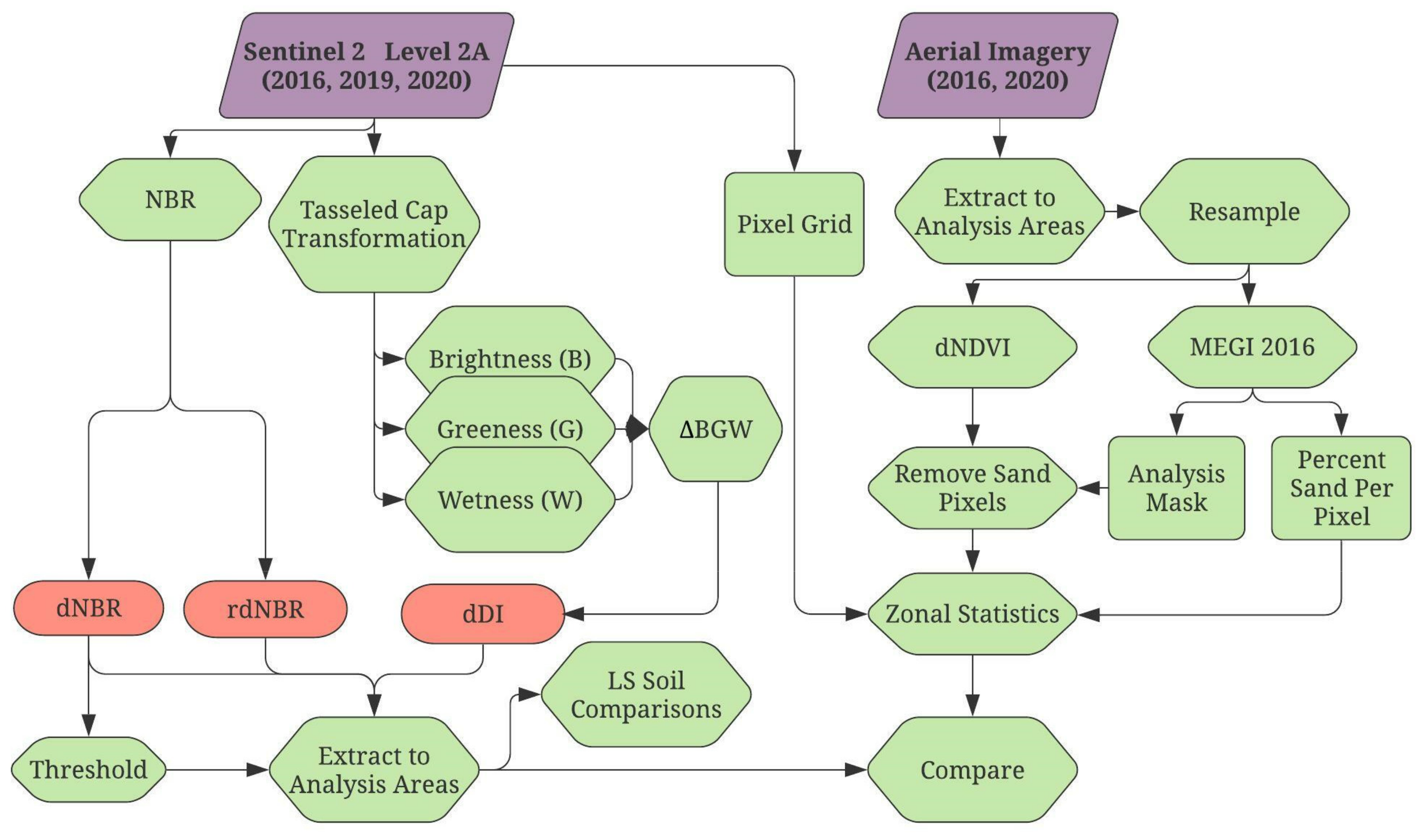
Data management, image analysis, and figure generation were primarily carried out in ArcGIS Pro (2.8), ERDAS Imagine 2020, and python environments. Sentinel 2 (S2) imagery and aerial imagery were used to assess fire severity (Table 2). High resolution aerial imagery with 4 spectral bands (RGB, NIR) for 2016 and 2020 was sourced from the most recent ortho-images from the State Government of South Australia. Pre-fire aerial imagery was resampled via cubic convolution to geometrically match the spatial resolution of 2020 aerial imagery. S2 imagery was sourced from the European Space Agency’s Copernicus Open Access Hub (https://scihub.copernicus.eu, accessed on 22 November 2021). Cloud free S2 imagery was acquired for before and after the fire event as well as to coincide with the dates of the high-resolution aerial imagery in 2016 and 2020. S2 imagery was resampled to the highest spatial resolution of 10m via cubic convolution. Level 2A imagery was acquired for the 2019 and 2020 imagery and Sen2Cor was used to apply atmospheric corrections for 2016 imagery [84]. All datasets were analysed in the Geocentric Datum of Australia 1994 (GDA94) with a Universal Transverse Mercator (UTM) datum in zone 53 South. An overview of the methods is shown in Figure 3.
2.3. Index Design
To transform imagery to the orthogonal TCT axes, bands are scaled to individual coefficients developed from representative imagery sets and combined in a linear equation. At the time of writing, specific coefficients for all bands within S2 ground reflectance imagery have not been published. Recently, some authors [85,86] have used coefficients developed for Landsat at-sensor reflectance products on S2 level-2A imagery. Others [87,88,89,90,91] have applied TCT coefficients to S2 level-2A data that were developed for at-sensor S2 (level-1C) imagery [43,92]. The spectral range and similarities of bands from Landsat and S2 bands are well documented [93,94,95], and the coefficients as developed by Crist [96] have been used in various studies using surface reflectance Landsat imagery [51,97,98,99]. For this study, coefficients were applied to S2 L2A bands (2490, 3560, 4665, 8842, 111610, 122190) and sourced from Landsat-derived coefficients for atmospherically corrected imagery [96] to derive TCB, TCG, and TCW.
dDI (Equation (1)) combines the Tasseled-cap indices (brightness, greenness, and wetness) into a single index value of transformed spectral distance and temporal change. In this application, a pre-disturbance image is used to assess the transformed spectral change that has occurred as a result of a fire.
where TCB′, TCG′, and TCW′ (Equation (2)) represent the transformed spectral difference in brightness, greenness, and wetness indices between the image dates, respectively.
The change in brightness values was found to be disproportionately high compared with the combined greenness and wetness in regions where the tree canopy was fully consumed and had bright soils; therefore, a scaling factor (0.5) was applied to the TCB’ output in the dDI calculation. Index values are rescaled to represent change in transformed reflectance values [84] by dividing by 10,000. The order of the equation has been shifted relative to the previously published DI equation [45] to ensure that areas disturbed resulted in a positive value. Larger index values indicate a likely disturbance event, with higher brightness and lower greenness and wetness giving greater positive values and severity. Low positive (<0.1) values indicate minimal changes in relative transformed spectral change with negative values or values close to 0 suggesting that brightness decreased or was unchanged relative to greenness and wetness and that disturbance was unlikely.
2.4. Satellite Fire Severity
The normalised burn ratio (NBR) (Equation (3)) was developed by Key et al. [28] and is the standard index used for burn severity and burnt area research and for large extent monitoring programs [100]. dNBR (Equation (4)) and rdNBR (Equation (5)) were calculated to compare conventional fire severity indices with the dDI. To align with the spectral resolution of Landsat [95] and previous applications of the index, NBR was computed with the bands 8842 and 122190 of S2 imagery.
Pre- and post-fire NBR were combined to calculate the differenced NBR (dNBR). dNBR values are the absolute change between images with positive pixel values indicating burnt areas, and higher values often interpreted as higher fire severity [39].
Miller et al. [18] developed the relativised dNBR (rdNBR) to better assess fire effects in pixels where pre-fire vegetation cover is low and an absolute measure of change would result in low values, regardless of total vegetation loss. Similar to dNBR, positive values indicate burnt areas and negative values represent areas with increased vegetation cover or vigour [37]. The dNBR value is relativised by dividing by square root of the absolute preNBR value and was calibrated based on in situ comparisons with fire severity [18].
As acknowledged in its development [18], low preNBR values will cause exceptionally large burn severity estimations in the resulting rdNBR index due to the division by a small value, causing significant overestimations of fire severity. For comparisons and visualisations in this analysis, the pixel values outside of 3 standard deviations (STDs) from the mean of rdNBR were considered outliers and removed.
2.5. High Resolution Aerial Assessment of Fire Severity
2.5.1. Representative Dune Sites
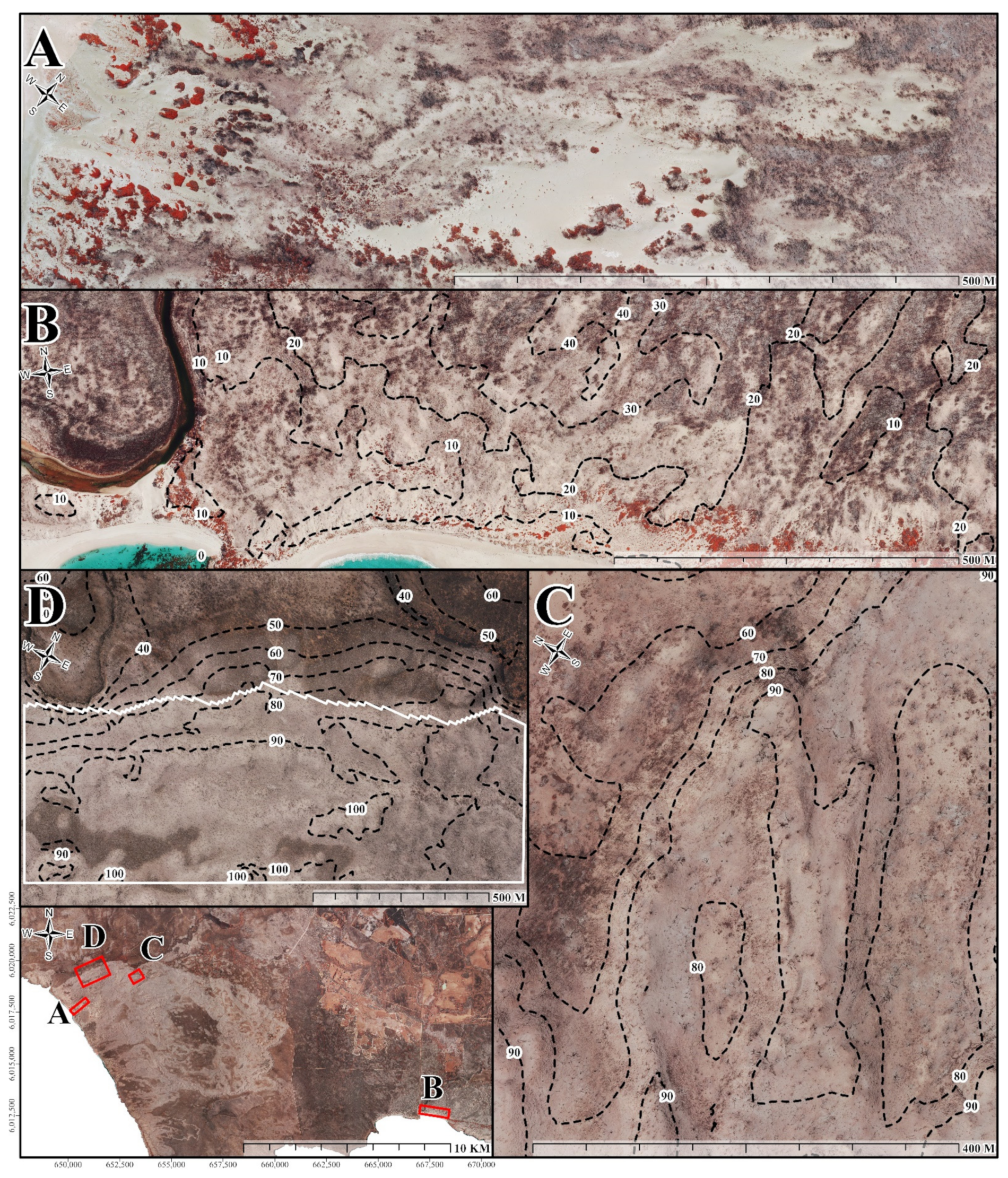
High spatial resolution aerial images provide a source of data that can be used to estimate burn severity, help track the recovery of vegetation [101,102,103,104,105,106], and corroborate observations from satellite imagery [104,107]. Aerial imagery from 2016 and 2020 (Table 2) was used to extract and measure vegetation loss in representative coastal dune systems (Figure 4 and Table 3). For further review of coastal dune types, see Hesp et al. [108]. Sites A and B are a mix of active and stabilised dune systems, characterised by high exposure to wave and aeolian energy. Both sites (A and B) were burnt in all regions except in the foredune areas (foremost depositional dune landward of the waterline). Before the fire event, Sites C and D were fully stabilised parabolic dunes characterised by thick mallee vegetation cover. The extent of site D was derived from the boundary of soil groups between Holocene sands and Pleistocene lowlands (GD and LP Table 1).
2.5.2. Measuring Fire Severity from Aerial Imagery
The Modified Excessive Green Index (MEGI) (Equation (6)) was calculated for the 2016 aerial imagery to distinguish between sand/soil and vegetation pixels in areas with a discontinuous canopy and exposed soils. MEGI emphasises the height of the green reflectance peak [109] and was used to isolate exposed soil and sand pixels after it was found that MEGI derived a larger spectral difference between sand and non-sand pixels (including green vegetation and woody bio-mass) than other NIR/RGB indices.
The non-sand classes, representing vegetation and other surface biomass, were merged to form an analysis mask. This focused the spectral analysis onto pixels that contained vegetation pre-fire in 2016, excluded previously active dune features or exposed soils, and gave a measurement of sand percentage per pixel for satellite index comparisons.
NDVI (Equation (7)) was calculated for 2016 and 2020 aerial images and differenced to show change in greenness and vegetation loss, producing a dNDVI (Equation (8)). The dNDVI image was masked to the MEGI-derived analysis mask to estimate canopy and vegetation loss, independent of exposed soil in the pre-fire image. An absolute measure of change (dNDVI) was chosen because non-vegetation pixels were excluded and did not necessitate the use of a relative index. Zonal statistics from the aerial imagery were taken according to the pixel size (10 m) and location of S2 imagery to produce average dNDVI values per pixel.
2.6. Comparisons of Satellite-Derived Fire Severity
Satellite indices were extracted to a focused analysis mask, composed of the extent of a thresholded dNBR image (>0.2) to remove unburnt pixels and a thresholded rdNBR image (3 STDs) to remove outliers. Spatial statistics were generated for satellite indices grouped by Landsystem (LS) Soil classifications [110] in regions with the highest burn severity indices, in dune formations, and within the protected National Park regions (Figure 5). Means and STDs of individual LS groups were compared to show differences between soil groups and the aggregate of all high burn severity LS groups (Figure 5). To compare the separability of index populations, a Welch’s t-test using Z-scores was completed comparing soil groups. Z-scores for individual soil groups were calculated based on aggregated mean and STDs from the total population of LS classes.
2.7. Comparisons to Aerial Fire Severity
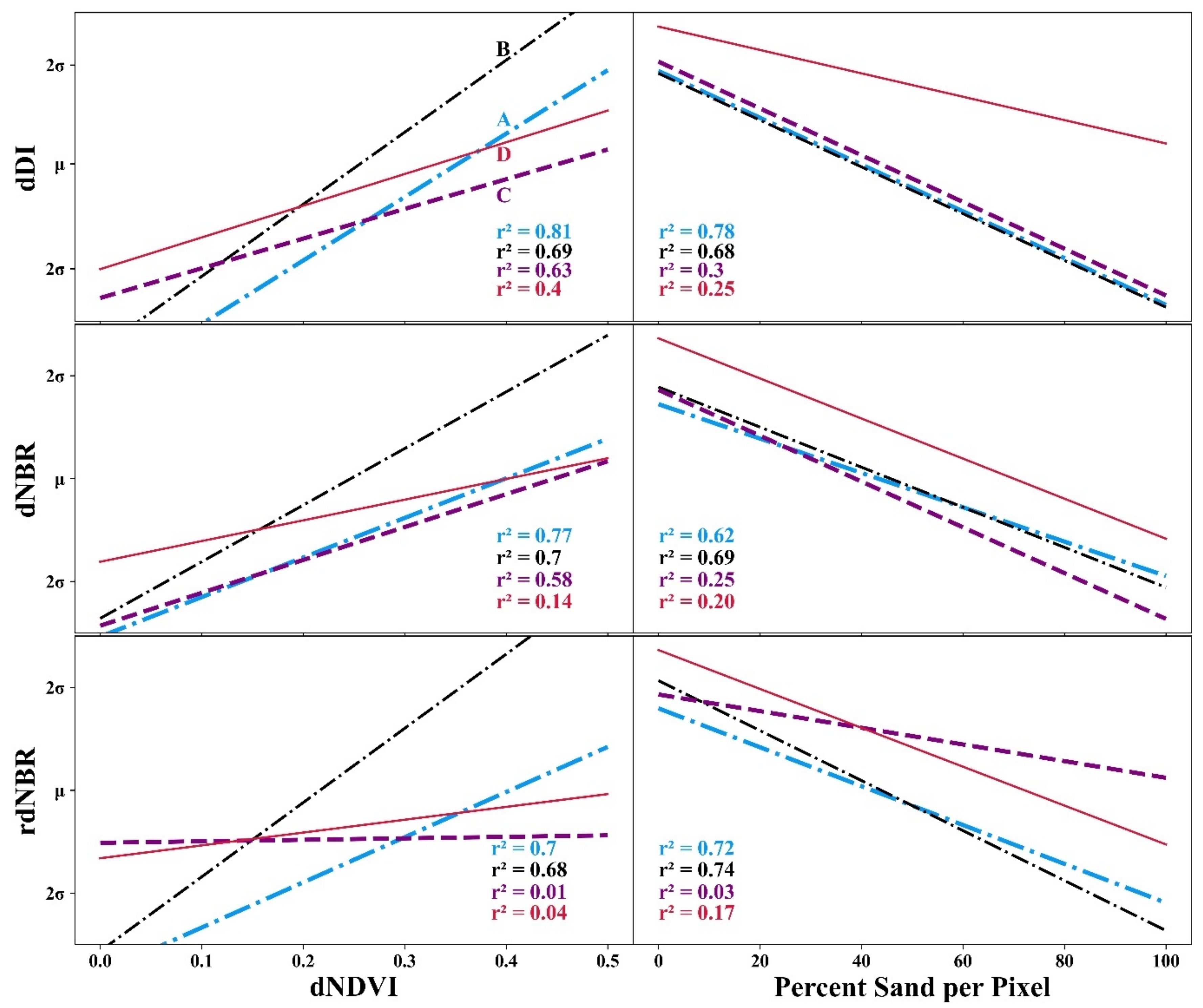
Satellite and aerial fire severity index values were compared with the four representative dune sites in the fire grounds on Kangaroo Island (Table 3 and Figure 4). The high-resolution aerial imagery provided the absolute measures of greenness lost from dNDVI values and the percentage of exposed sand per pre-fire pixel. Trend lines and coefficient of determination (r2) values were generated to show the relationship between satellite-derived indices and the information extracted from aerial imagery: the absolute measure of greenness and vegetation loss independent of exposed sand and the total percentage per pixel of sand exposed pre-fire.
3. Results
3.1. Differenced Disturbance Index
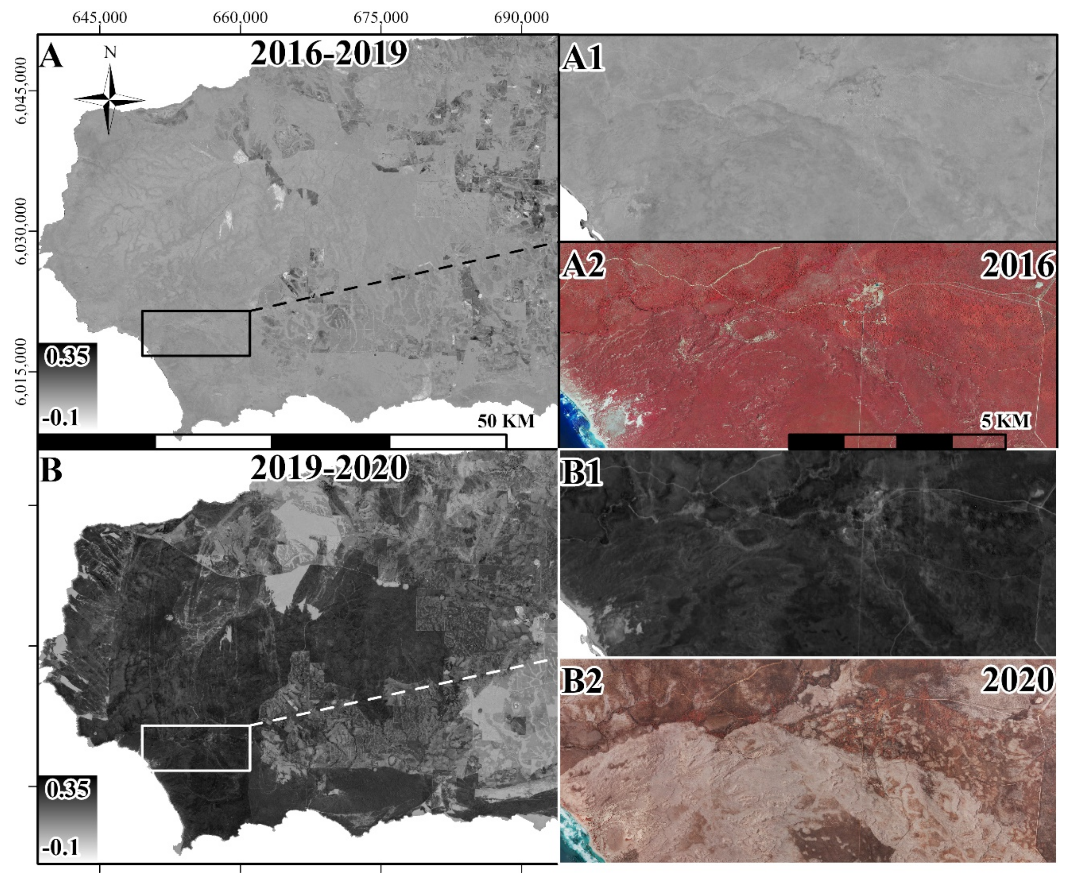
The outputs from dDI show the difference in transformed spectral distance between two dates, with a larger index value indicating a greater spectral difference and a larger deviation from previous pixel values. Figure 6 shows the results of two separate dDI calculations between two distinct time periods, 2016 to 2019 (panel A) and 2019 to 2020 (panel B). From 2016 to 2019, few large disturbance events are detected with most areas showing low dDI values. The largest dDI values between 2016 and 2019 are in agricultural areas and are likely a result of irrigation and land use changes. Panel B shows the results of the 2019/2020 fires, with high index values shown in darker pixels. Panels B1 and B2 of Figure 6 show the dDI values across different soils and landscape types. The clear boundary between light and darker soils is visible in B2 and shown in Figure 2 as the border between the landscape units of Northcote’s Gantheaume Dunes and Gosse Plateau.
3.2. Comparisons of Satellite Fire Severity
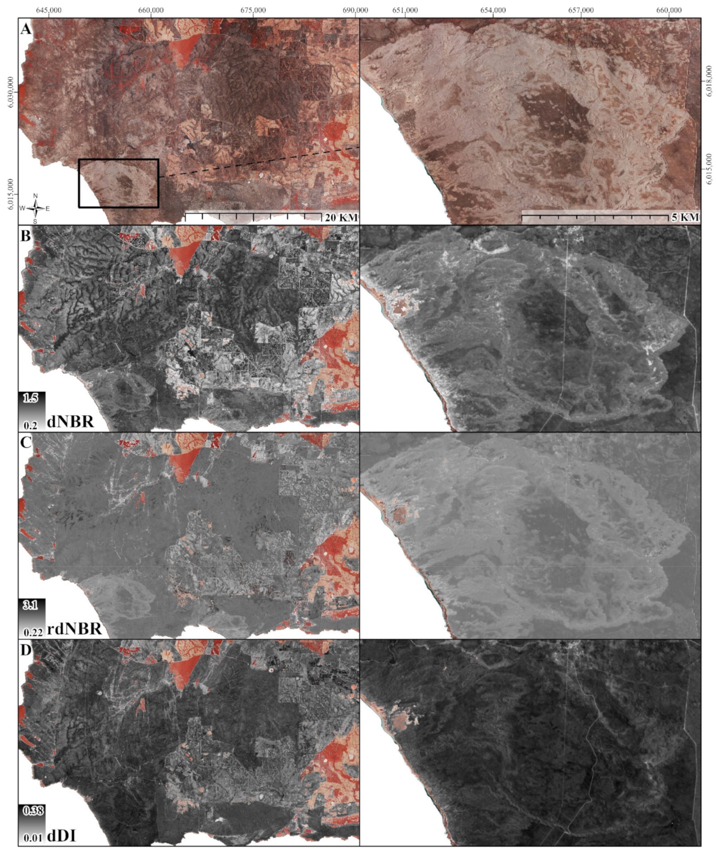
To illustrate the differences in fire severity, imagery from 2020 and change over time indices from 2016 and 2020 are shown in Figure 7. Fire severity is derived from the two forms of NBR, with its absolute and relative version and a dDI image. All indices are extracted to the extent of a dNBR threshold (>0.2) and presented in 3 STDs from white to black, showing low to high fire severity. In the inset maps of Figure 7, the boundaries between the brighter and darker soils (Figure 8) are visible in both NBR fire severity indices, showing a lower relative value as a result of soil brightness. Compared with the index output from dDI, the effects of soil brightness have been removed and there is a consistent measure of high fire severity between the two soil groups and across the firegrounds. In the left-hand panels of Figure 7B, the highest values in dNBR correspond to the riverine soils, seen in the dendritic pattern of the dissected tableland and in areas of agroforestry in the centre of the panel.
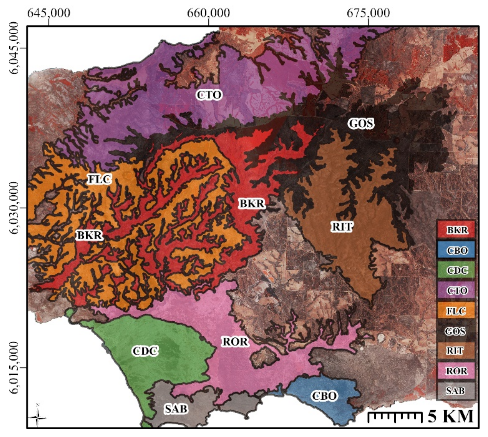
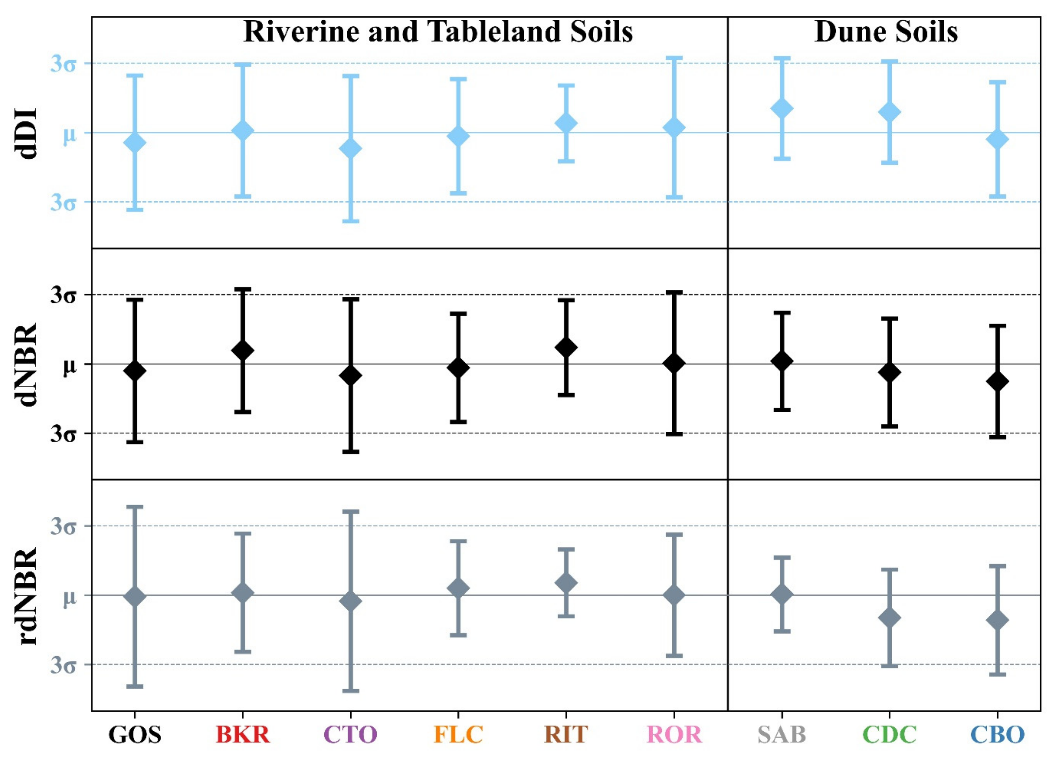
Figure 4 shows the extent of each Landsystem (LS) soil classification used in Figure 9 to show the spatial variability of means and standard deviations per LS group. Even at the aggregated LS unit, soil brightness decreases the severity of both NBR indices in the bright dune soils. The SAB LS group is considered a dune formation although it is characterised by darker Pleistocene calcarenite overlain by shallow sandy Holocene deposits [110], meaning its soil reflectance is considerably darker than adjacent dune formations. The resulting NBR indices suggest higher severity (Figure 9) in these regions due to its predominant darker soil profile (and therefore surface colour). dDI shows similar relative fire severity for the tableland and riverine soil groups, with the dune soils reflecting the complete loss of canopy and vegetation across the dune soils of CDC and SAB. The results of a Welch’s t-test indicate that all compared indices exhibit significant differences in their population’s mean, with the Pearson’s correlation showing their divergence presented in Appendix B, Table A2.
3.3. Comparison with Aerial Fire Severity
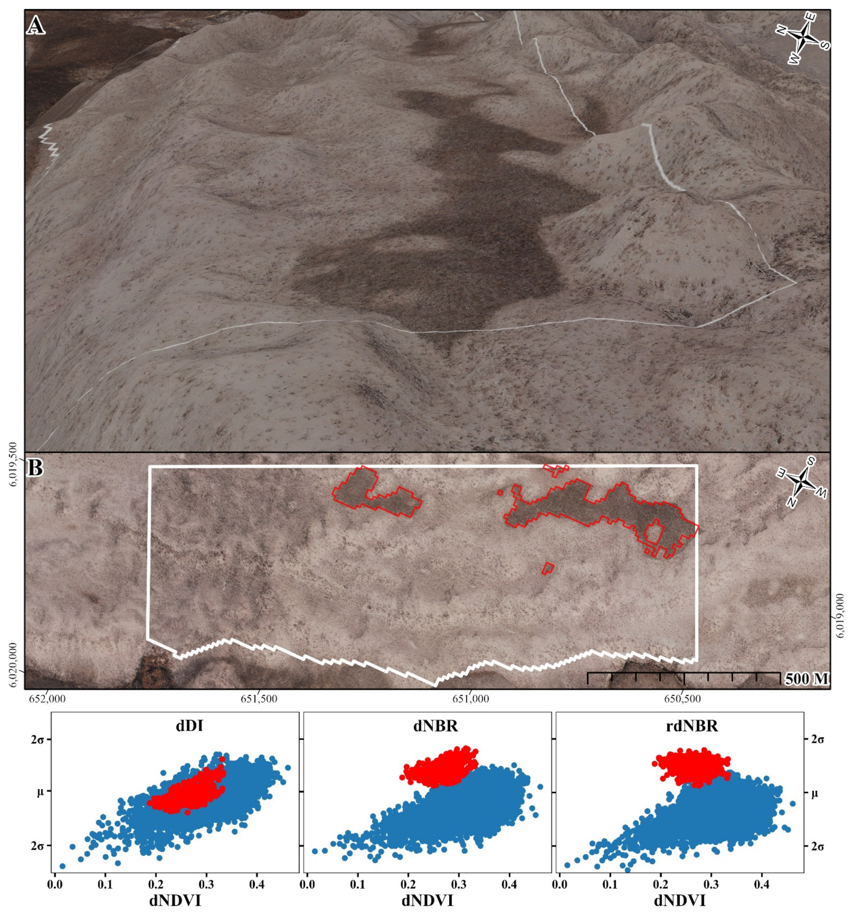
Figure 10 illustrates the positive association between dNDVI and satellite fire severity indices in the representative dune sites A–D (Figure 4), suggesting that all three indices track loss of greenness with increasing index values. The negative association of index value and increasing sand percentage per pixel in Figure 10 shows that all severity values decrease as the percentage of sand per pixel increases.
Figure 11 demonstrates the resulting effects of soil brightness on index value within site D. Interdune swales are low points in dune landscapes that are more sheltered environments, characterised by increased moisture, higher humus and organic surface deposits, lower wind areas, accumulation and trapping of surface water, and commonly, a different vegetation community than in adjacent higher areas, often resulting in darker soils [111]. The canopy loss is uniform within this area according to the high-resolution aerial imagery, suggesting very high severity throughout site D. The darker soils located within the interdune swale have substantially higher index values in both NBR (Figure 11) indices, contrasted to the more consistent rating of fire severity from dDI that aligns with full canopy consumption.
4. Discussion
Kangaroo Island is a highly heterogenous landscape, exhibiting multiple broad soil groups and vegetation communities. The fire in the summer of 2019/2020 affected large swathes of the island and many of the predominant vegetation communities and soil groups. Desktop studies of the effects of the fire have shown that large portions of the island exhibited very high fire severity [30,112], although those studies assessed the fire impacts on the Holocene dunes (Figure 1) to be relatively less severe due to fixed severity thresholds. It has been well documented that NBR values are influenced by changes in soil colour, often attributed to residual char or ash and differing soil types [13,100]. The results of this work show that the fire severity values from NBR are influenced by soil type and brightness, both at the local level (Figure 11) and across the broad soil groups (Figure 5 and Figure 9). The border between the bright carbonate rich sands of the Holocene dune formations and the darker Pleistocene lowland soils with verdant riverine woodlands is clearly visible within the imagery (Figure 7 and Figure 8) and NBR-based indices (Figure 7), resulting in differential classifications of fire severity in Government reports [112]. The results of this work show that uncalibrated coarsely applied severity thresholds will result in differential fire severity more closely aligned with differences in soil brightness and predominant vegetation communities than actual effects of fire.
The differenced Disturbance Index (dDI) presented in this work computes the transformed spectral difference between two dates, measuring the effects of a disturbance such as fire. The results show that dDI is less affected by soil brightness and corresponds to the absolute measures of greenness loss irrespective of varying canopy cover. dDI allows for the effects of soil brightness to be mitigated with a scaling factor to reduce its overall contribution to the resulting index, and the applied factor (0.5) shows good results for the heterogenous soils and landscapes of Kangaroo Island. Whereas others have successfully applied the normalised version of DI [45,46,47,48,49,50,51,113,114], the prerequisite information of representative pixel values of target landscapes for normalisation limits its broadscale application. The dDI presented here is a direct pixel to pixel comparison, requiring no region-specific adjusted thresholds or mean values for normalisation. The index output of dDI denotes the magnitude of change between two dates, with the highest index values indicating a complete consumption of canopy and removal of vegetation. The three outputs from the Tasseled Cap Transform; TCB, TCG, and TCW represent the three surface components of brightness, greenness and wetness. The linear combination of these three surface components models the vegetation stand replacing nature of severe fires by an increase in brightness and non-vegetation reflectance and decreases in greenness and wetness or spectra associated with vegetation’s reflectance. dDI incorporates all spectral information transformed with TCT coefficients within satellite imagery, harnessing the benefits of the enlarged spectrum from SWIR, NIR, and RGB bands. Combined, SWIR and NIR bands are sensitive to the characteristic effects of fires, showing changes in forest structure, soils, and moisture content [26] and the variations in greenness or chlorophyl from the NIR [29,34]. The RGB regions of the EM contains often discarded data showing the effects of disturbances which can be helpful for Mediterranean or semi-arid to arid environments or areas with lower NIR reflectance, illustrated in pre- and post-disturbance comparisons of true colour imagery.
Certain limitations of dDI have been shown by the methods and results of this work. These are reviewed below with suggested areas for improvement resulting from uncertainty around TCT coefficients, large spectral changes resulting from non-disturbance (land use) changes, and the decreasing severity index value as a result of discontinuous canopy coverage.
As reviewed in Section 2.3, TCT coefficients have not been published for atmospherically corrected S2 imagery, and Landsat’s surface reflectance coefficients [96] do not cover all S2 bands. Whereas certain authors have used at-sensor-derived coefficients on surface reflectance S2 imagery [87,88,89,90,91], in a multi-temporal change application, the ever-changing effects of atmosphere result in inconsistent indices of brightness, greenness, and wetness that are directly a result of fluctuating atmospheric conditions. Although the exact effects onto index values such as dDI are not fully understood, Crist et al. [42] suggests that changing atmospheric conditions will alter subsequent results derived from TCT indices. The development of coefficients for all S2 (level-2a) bands will improve the consistency of spectral information derived from combinations of TCT indices such as dDI and ensure its fidelity when compared with other sensors’ surface reflectance products in a time series.
The high-resolution aerial imagery used in this work (<40 cm) quantifies the spectral differences between burnt and unburnt pixels and provides an estimation of the absolute greenness and canopy loss following fire. Due to its 2D resolution, it is unable to provide a detailed estimate of vegetation structural changes or net amounts of biomass loss which would improve severity estimates. Additionally, in regions that have experienced large spectral changes resulting from shifts in land use (Figure 6A), dDI values suggest a disturbance due to the large spectral difference between dates. Indices of change to vegetation from passive optical sensors, such as Sentinel 2, are derived from changes in the spectral reflectance of pixels and measure differences in object chemistry before and after a fire. However, changes observed in near simultaneously acquired SAR imagery, particularly in cross-polarized backscatter, indicate changes to object structure resulting from fire [115,116,117]. Thus, it is likely that a combination of indices such as dDI with differences in calibrated cross polarized backscatter from sensors such as Sentinel 1, NovaSAR1, and the future NISAR are likely to improve an understanding of the impact of fire on natural landscapes such as those in coastal dunes. The addition of simultaneous texture information could greatly increase the ability of severity estimates in areas with sparse canopies and reduce the effect of decreasing pre-fire canopy coverage and post-fire severity estimates as shown in Figure 10 and Section 3.3. Additional datasets such as the fractional cover products from Digital Earth Australia (DEA) [118] could be used to adjust or scale severity indices according to the pixel’s percentage of pre-fire exposed soils, improving severity estimates in areas with sparse vegetation cover. Fractional cover is derived from endmembers of representative pixels and spectral unmixing, deriving percentage per pixel of bare ground, green vegetation, and woody biomass [119]. If sufficiently validated and calibrated, there is significant potential to implement a fire severity mapping method that measures the severity of a fire as a result of its spectral and textural changes and leverages the vast datasets and processing capabilities available through initiatives such as DEA’s Open Data Cube (ODC) [120,121].
The suitability of fire severity indices are often evaluated by comparisons with local observations of the CBI [27,28,29,122], a linear combination of up to 23 in situ factors of which the effects of soils is only one component [18]. Further investigation of the suitability of satellite-derived spectral indices to varied landscapes requires studies to validate and calibrate their accuracy and precision for diverse vegetation communities and soil variability. The inclusion of structural estimates from active sensors on airborne platforms could provide high-resolution validation datasets for diverse calibration sites and reduce the inherent subjectivity of conventional in situ burn severity estimates. Research has shown that active sensors on airborne platforms, either in the form of airborne LIDAR [123] or airborne synthetic aperture radar (SAR) [124], can significantly increase the understanding of structural and 3D changes as a result of fire. Within diverse and representative calibration sites, these sensors could assess net structural changes caused by fire and improve the accuracy of space-based fire severity estimates in heterogenous environments.
Coastal dunes are dynamic and resilient systems that are continually adjusting to disturbances and extreme events [125]. The stratigraphy-based research suggesting dune destabilisations after fires [62,63,64,65,66,67,68,69,70,71] has not been confirmed by contemporary observations [32,33,53], but the consequences of increasing frequency [30] and severity [8] of fires may result in altered landscape morphology and dominant vegetation communities [10]. Specific to Kangaroo Island, the highly fire-adapted vegetation community is likely a result of the evolution in its fire regime since colonisation. The pre-European fire regime of Kangaroo Island is thought to be driven by dry lightning strokes characterised by infrequent but severe fires [83], as the archaeological record indicates the island was uninhabited by humans for at least 400 years [126,127], with others suggesting closer to 2500 years BP [128]. Bauer [81] suggests that fire intensity and frequency were dramatically scaled up after European colonisation to facilitate land clearance and that non-developed areas of the island may be a modern artifact reflecting a shift in fire regimes. The implications of this suggest that the island’s vegetated areas may be less susceptible to landscape destabilisation from fires as the vegetation communities are highly adapted to frequent and severe fire.
5. Conclusions
This paper provides a new application of a temporally differenced Disturbance Index (dDI) based on the Tasseled Cap Transformation (TCT) features of brightness, greenness and wetness which improves burn severity measurements for heterogeneous environments. Satellite-derived fire severity indices are compared with high resolution multi-spectral aerial imagery to show the relationship between loss of greenness and canopy consumption and fire severity in representative dune sites across Kangaroo Island. dDI calculates, at the pixel level, the transformed spectral difference between two image dates and quantifies severity within burnt areas. This is the first application of the dDI in a direct pixel to pixel comparison, not requiring the use of prerequisite image or landscape-derived statistics as implemented in previous applications. Comparisons with both versions of the Normalised Burn Ratio (NBR) indicate that dDI is less affected by soil brightness at local and regional scales; therefore, it is able to detect and measure high burn severity in dunes on Kangaroo Island.
Fire severity is suggested to be one possible trigger for landscape instability and a possible initiation mechanism for transgressive dune phases, but coastal dune landscapes have characteristics that display the precise limitations of the conventional NBR-derived indices: heterogeneity, discontinuous canopies, and bright soils.
It is unclear as to what effect the widespread use of NBR-based severity estimates influence the responses of Governments or policy makers for recovery and fuel load management decisions. If resource allocation or response plans are shaped by broadly applied uncalibrated fire severity thresholds, then there is a significant risk of under-assessing areas that have experienced a high severity fire.
Improving the estimations of fire severity in coastal dune and other heterogenous systems will better illustrate the true effects of fires in these landscapes and aid in studies of their subsequent recovery or destabilisation.
Author Contributions
Conceptualisation, M.D.D., D.B., G.M.d.S. and P.A.H.; methodology, M.D.D. and D.B.; software, M.D.D.; validation, M.D.D.; formal analysis, M.D.D.; investigation, M.D.D. and D.B.; resources, M.D.D., D.B., G.M.d.S. and P.A.H.; data curation, M.D.D.; writing—original draft preparation, M.D.D.; writing—review and editing, M.D.D., D.B., G.M.d.S. and P.A.H.; visualisation, M.D.D., D.B., G.M.d.S. and P.A.H.; supervision, D.B., G.M.d.S. and P.A.H.; project administration, M.D.D.; funding acquisition, P.A.H., M.D.D., D.B. and G.M.d.S. All authors have read and agreed to the published version of the manuscript.
Funding
This research was funded by Flinders University SEED grant and the Department of Environment and Water (DEW), South Australia.
Data Availability Statement
Aerial imagery can be accessed via Mapland through DEW. Aerial imagery from 2020 is a restricted use dataset requiring special approvals for distribution. Sentinel 2 imagery is freely available through ESA web portal. Landsystem (LS) soil information and spatial data can be accessed at http://location.sa.gov.au/lms/Reports/ReportMetadata.aspx?p_no=1103&pu=y&pa=dewnr&pu=y, accessed on 23 November 2021. Broad soil classification based on Northcote’s and shown in Figure 2 is available at: https://www.asris.csiro.au/themes/Atlas.html, accessed on 23 November 2021. The following web map corresponding to Figure 4 is available online at https://arcg.is/0j1T450, accessed on 23 November 2021.
Acknowledgments
Special thanks to DEW and Flinders University for funding of the on-going research on Kangaroo Island listed above. Additionally, to Flinders University for the on-going PhD scholarship and project funding. Special thanks to Enya Chitty, Joram Downes, Michael Hillman and Ben Perry from Flinders University and Ali Turner from DEW for field help and on-going project support.
Conflicts of Interest
The authors declare no conflict of interest. The funders had no role in the design of the study; in the collection, analyses, or interpretation of data; in the writing of the manuscript, or in the decision to publish the results.
Appendix A

Table A1.
Showing the Landsystem (LS) Unit used to compare fire severity in Figure 5 and Figure 9. All descriptions are available at https://data.environment.sa.gov.au/, accessed on 23 November 2021.
Table A1.
Showing the Landsystem (LS) Unit used to compare fire severity in Figure 5 and Figure 9. All descriptions are available at https://data.environment.sa.gov.au/, accessed on 23 November 2021.
Appendix B
Table A2.
Pearson’s R correlation coefficient as derived from the Welch’s t-test comparing Z scores for index values grouped by Landsystem (LS) Soil groups. Index values from the differenced Disturbance Index (dDI), differenced Normalised Burn Ratio (NBR) and the relativised differenced Normalised Burn Ratio (rdNBR) are compared in pairs to show significant differences in population means (all pairs assessed to be significant by p value 0.05 except highlighted and bold). Higher values indicate larger deviations from the compared means of individual indices.
| LS | dDI-dNBR | dDI-rdNBR | dNBR-rdNBR |
|---|---|---|---|
| GOS | 0.08 | 0.18 | 0.11 |
| BKR | 0.28 | 0.04 | 0.27 |
| CTO | 0.11 | 0.20 | 0.10 |
| FLC | 0.00 | 0.31 | 0.32 |
| RIT | 0.25 | 0.12 | 0.16 |
| ROR | 0.09 | 0.12 | 0.03 |
| SAB | 0.55 | 0.65 | 0.07 |
| CDC | 0.64 | 0.80 | 0.38 |
| CBO | 0.27 | 0.44 | 0.20 |
References
- Seidl, R.; Thom, D.; Kautz, M.; Martin-Benito, D.; Peltoniemi, M.; Vacchiano, G.; Wild, J.; Ascoli, D.; Petr, M.; Honkaniemi, J.; et al. Forest disturbances under climate change. Nat. Clim. Chang. 2017, 7, 395–402. [Google Scholar] [CrossRef] [Green Version]
- Keeley, J.E. Seed-Germination Patterns in Fire-Prone Mediterranean-Climate Regions. In Ecology and Biogeography of Mediterranean Ecosystems in Chile, California, and Australia; Arroyo, M.T.K., Zedler, P.H., Fox, M.D., Eds.; Springer: New York, NY, USA, 1995; pp. 239–273. [Google Scholar]
- Wellington, A.; Noble, I. Post-fire recruitment and mortality in a population of the mallee Eucalyptus incrassata in semi-arid, south-eastern Australia. J. Ecol. 1985, 73, 645–656. [Google Scholar] [CrossRef]
- Wright, B.R.; Clarke, P.J. Fire regime (recency, interval and season) changes the composition of spinifex (Triodia spp.)-dominated desert dunes. Aust. J. Bot. 2007, 55, 709–724. [Google Scholar] [CrossRef]
- Barbero, R.; Abatzoglou, J.T.; Pimont, F.; Ruffault, J.; Curt, T. Attributing Increases in Fire Weather to Anthropogenic Climate Change Over France. Front. Earth Sci. 2020, 8, 104. [Google Scholar] [CrossRef]
- Keeley, J.E.; Syphard, A.D. Climate Change and Future Fire Regimes: Examples from California. Geosciences 2016, 6, 37. [Google Scholar] [CrossRef] [Green Version]
- Turton, S.M. Geographies of bushfires in Australia in a changing world. Geogr. Res. 2020, 58, 313–315. [Google Scholar] [CrossRef]
- Tran, B.N.; Tanase, M.A.; Bennett, L.T.; Aponte, C. High-severity wildfires in temperate Australian forests have increased in extent and aggregation in recent decades. PLoS ONE 2020, 15, e0242484. [Google Scholar] [CrossRef] [PubMed]
- Storey, E.A.; Stow, D.A.; O’Leary, J.F.; Davis, F.W.; Roberts, D.A. Does short-interval fire inhibit postfire recovery of chaparral across southern California? Sci. Total Environ. 2021, 751, 142271. [Google Scholar] [CrossRef] [PubMed]
- Bennett, L.T.; Bruce, M.J.; MacHunter, J.; Kohout, M.; Tanase, M.A.; Aponte, C. Mortality and recruitment of fire-tolerant eucalypts as influenced by wildfire severity and recent prescribed fire. For. Ecol. Manag. 2016, 380, 107–117. [Google Scholar] [CrossRef]
- Levin, N.; Levental, S.; Morag, H. The effect of wildfires on vegetation cover and dune activity in Australia’s desert dunes: A multisensor analysis. Int. J. Wildland Fire 2012, 21, 459–475. [Google Scholar] [CrossRef]
- Schoennagel, T.; Smithwick, E.A.; Turner, M.G. Landscape heterogeneity following large fires: Insights from Yellowstone National Park, USA. Int. J. Wildland Fire 2009, 17, 742–753. [Google Scholar] [CrossRef]
- Turner, M.G.; Hargrove, W.W.; Gardner, R.H.; Romme, W.H. Effects of Fire on Landscape Heterogeneity in Yellowstone-National-Park, Wyoming. J. Veg. Sci. 1994, 5, 731–742. [Google Scholar] [CrossRef] [Green Version]
- Coppoletta, M.; Merriam, K.E.; Collins, B.M. Post-fire vegetation and fuel development influences fire severity patterns in reburns. Ecol. Appl. 2016, 26, 686–699. [Google Scholar] [CrossRef] [PubMed]
- Mathews, L.E.H.; Kinoshita, A.M. Vegetation and Fluvial Geomorphology Dynamics after an Urban Fire. Geosciences 2020, 10, 317. [Google Scholar] [CrossRef]
- Chuvieco, E.; Mouillot, F.; van der Werf, G.R.; San Miguel, J.; Tanase, M.; Koutsias, N.; Garcia, M.; Yebra, M.; Padilla, M.; Gitas, I.; et al. Historical background and current developments for mapping burned area from satellite Earth observation. Remote Sens. Environ. 2019, 225, 45–64. [Google Scholar] [CrossRef]
- Gibson, R.; Danaher, T.; Hehir, W.; Collins, L. A remote sensing approach to mapping fire severity in south-eastern Australia using sentinel 2 and random forest. Remote Sens. Environ. 2020, 240, 111702. [Google Scholar] [CrossRef]
- Miller, J.D.; Thode, A.E. Quantifying burn severity in a heterogeneous landscape with a relative version of the delta Normalized Burn Ratio (dNBR). Remote Sens. Environ. 2007, 109, 66–80. [Google Scholar] [CrossRef]
- Klinger, R.; McKinley, R.; Brooks, M. An evaluation of remotely sensed indices for quantifying burn severity in arid ecoregions. Int. J. Wildland Fire 2019, 28, 951–968. [Google Scholar] [CrossRef]
- Seydi, S.T.; Akhoondzadeh, M.; Amani, M.; Mahdavi, S. Wildfire Damage Assessment over Australia Using Sentinel-2 Imagery and MODIS Land Cover Product within the Google Earth Engine Cloud Platform. Remote Sens. 2021, 13, 220. [Google Scholar] [CrossRef]
- Royal Commission into National Natural Disaster Arrangements. Interim Observations; Commonwealth of Australia: Canberra, Australia, 2020.
- Aponte, C.; de Groot, W.J.; Wotton, B.M. Forest fires and climate change: Causes, consequences and management options. Int. J. Wildland Fire 2016, 25, i–ii. [Google Scholar] [CrossRef]
- Boucher, J.; Beaudoin, A.; Hebert, C.; Guindon, L.; Bauce, E. Assessing the potential of the differenced Normalized Burn Ratio (dNBR) for estimating burn severity in eastern Canadian boreal forests. Int. J. Wildland Fire 2017, 26, 32–45. [Google Scholar] [CrossRef]
- Russell-Smith, J.; Edwards, A.C. Seasonality and fire severity in savanna landscapes of monsoonal northern Australia. Int. J. Wildland Fire 2006, 15, 541–550. [Google Scholar] [CrossRef]
- Keeley, J.E. Fire intensity, fire severity and burn severity: A brief review and suggested usage. Int. J. Wildland Fire 2009, 18, 116–126. [Google Scholar] [CrossRef]
- Veraverbeke, S.; Gitas, I.; Katagis, T.; Polychronaki, A.; Somers, B.; Goossens, R. Assessing post-fire vegetation recovery using red-near infrared vegetation indices: Accounting for background and vegetation variability. ISPRS J. Photogramm. Remote Sens. 2012, 68, 28–39. [Google Scholar] [CrossRef] [Green Version]
- Parks, S.A.; Dillon, G.K.; Miller, C. A new metric for quantifying burn severity: The relativized burn ratio. Remote Sens. 2014, 6, 1827–1844. [Google Scholar] [CrossRef] [Green Version]
- Key, C.; Benson, N. Landscape assessment: Ground measure of severity, the Composite Burn Index; And remote sensing of severity, the Normalized Burn Ratio. In FIREMON: Fire Effects Monitoring and Inventory System; US Department of Agriculture, Forest Service, Rocky Mountain Research Station: Fort Collins, CO, USA, 2005; Volume 2004. [Google Scholar]
- Tran, B.N.; Tanase, M.A.; Bennett, L.T.; Aponte, C. Evaluation of Spectral Indices for Assessing Fire Severity in Australian Temperate Forests. Remote Sens. 2018, 10, 1680. [Google Scholar] [CrossRef] [Green Version]
- Bonney, M.T.; He, Y.H.; Myint, S.W. Contextualizing the 2019-2020 Kangaroo Island Bushfires: Quantifying Landscape-Level Influences on Past Severity and Recovery with Landsat and Google Earth Engine. Remote Sens. 2020, 12, 3942. [Google Scholar] [CrossRef]
- Hislop, S.; Jones, S.; Soto-Berelov, M.; Skidmore, A.; Haywood, A.; Nguyen, T.H. Using Landsat Spectral Indices in Time-Series to Assess Wildfire Disturbance and Recovery. Remote Sens. 2018, 10, 460. [Google Scholar] [CrossRef] [Green Version]
- Shumack, S.; Hesse, P. Assessing the geomorphic disturbance from fires on coastal dunes near Esperance, Western Australia: Implications for dune de-stabilisation. Aeolian Res. 2018, 31, 29–49. [Google Scholar] [CrossRef]
- Shumack, S.; Hesse, P.; Turner, L. The impact of fire on sand dune stability: Surface coverage and biomass recovery after fires on Western Australian coastal dune systems from 1988 to 2016. Geomorphology 2017, 299, 39–53. [Google Scholar] [CrossRef]
- Massetti, A.; Rudiger, C.; Yebra, M.; Hilton, J. The Vegetation Structure Perpendicular Index (VSPI): A forest condition index for wildfire predictions. Remote Sens. Environ. 2019, 224, 167–181. [Google Scholar] [CrossRef]
- Key, C.H.; Benson, N.C. Landscape assessment (LA). In FIREMON: Fire Effects Monitoring and Inventory System; General Technical Report, RMRS-GTR-164-CD; Lutes, D.C., Keane, R.E., Caratti, J.F., Key, C.H., Benson, N.C., Sutherland, S., Gangi, L.J., Eds.; US Department of Agriculture, Forest Service, Rocky Mountain Research Station: Fort Collins, CO, USA, 2006; p. LA-1-55, 164. [Google Scholar]
- Norton, J.; Glenn, N.; Germino, M.; Weber, K.; Seefeldt, S. Relative suitability of indices derived from Landsat ETM+ and SPOT 5 for detecting fire severity in sagebrush steppe. Int. J. Appl. Earth Obs. Geoinf. 2009, 11, 360–367. [Google Scholar] [CrossRef]
- Miller, J.D.; Knapp, E.E.; Key, C.H.; Skinner, C.N.; Isbell, C.J.; Creasy, R.M.; Sherlock, J.W. Calibration and validation of the relative differenced Normalized Burn Ratio (RdNBR) to three measures of fire severity in the Sierra Nevada and Klamath Mountains, California, USA. Remote Sens. Environ. 2009, 113, 645–656. [Google Scholar] [CrossRef]
- Fassnacht, F.E.; Schmidt-Riese, E.; Kattenborn, T.; Hernandez, J. Explaining Sentinel 2-based dNBR and RdNBR variability with reference data from the bird’s eye (UAS) perspective. Int. J. Appl. Earth Obs. Geoinf. 2021, 95, 102262. [Google Scholar] [CrossRef]
- Soverel, N.O.; Perrakis, D.D.B.; Coops, N.C. Estimating burn severity from Landsat dNBR and RdNBR indices across western Canada. Remote Sens. Environ. 2010, 114, 1896–1909. [Google Scholar] [CrossRef]
- Wang, C.; Glenn, N.F. Estimation of fire severity using pre- and post-fire LiDAR data in sagebrush steppe rangelands. Int. J. Wildland Fire 2009, 18, 848–856. [Google Scholar] [CrossRef] [Green Version]
- Kauth, R.J.; Thomas, G.S. The tasselled cap—A graphic description of the spectraltemporal development of agricultural crops as seen by Landsat. In Proceedings of the Symposium on Machine Processing of Remotely Sensed Data, West Lafayette, IN, USA, 29 June–1 July 1976; pp. 41–51. [Google Scholar]
- Crist, E.P.; Cicone, R.C. A Physically-Based Transformation of Thematic Mapper Data—The Tm Tasseled Cap. IEEE Trans. Geosci. Remote Sens. 1984, 22, 256–263. [Google Scholar] [CrossRef]
- Shi, T.T.; Xu, H.Q. Derivation of Tasseled Cap Transformation Coefficients for Sentinel-2 MSI At-Sensor Reflectance Data. IEEE J. Sel. Top. Appl. Earth Obs. Remote Sens. 2019, 12, 4038–4048. [Google Scholar] [CrossRef]
- Marcos, B.; Goncalves, J.; Alcaraz-Segura, D.; Cunha, M.; Honrado, J.P. A Framework for Multi-Dimensional Assessment of Wildfire Disturbance Severity from Remotely Sensed Ecosystem Functioning Attributes. Remote Sens. 2021, 13, 780. [Google Scholar] [CrossRef]
- Healey, S.P.; Cohen, W.B.; Yang, Z.Q.; Krankina, O.N. Comparison of Tasseled Cap-based Landsat data structures for use in forest disturbance detection. Remote Sens. Environ. 2005, 97, 301–310. [Google Scholar] [CrossRef]
- Huang, Z.B.; Cao, C.X.; Chen, W.; Xu, M.; Dang, Y.F.; Singh, R.P.; Bashir, B.; Xie, B.; Lin, X.J. Remote Sensing Monitoring of Vegetation Dynamic Changes after Fire in the Greater Hinggan Mountain Area: The Algorithm and Application for Eliminating Phenological Impacts. Remote Sens. 2020, 12, 156. [Google Scholar] [CrossRef] [Green Version]
- Baumann, M.; Ozdogan, M.; Wolter, P.T.; Krylov, A.; Vladimirova, N.; Radeloff, V.C. Landsat remote sensing of forest windfall disturbance. Remote Sens. Environ. 2014, 143, 171–179. [Google Scholar] [CrossRef]
- DeRose, R.J.; Long, J.N.; Ramsey, R.D. Combining dendrochronological data and the disturbance index to assess Engelmann spruce mortality caused by a spruce beetle outbreak in southern Utah, USA. Remote Sens. Environ. 2011, 115, 2342–2349. [Google Scholar] [CrossRef]
- Liu, Q.S.; Liu, G.H.; Huang, C. Monitoring desertification processes in Mongolian Plateau using MODIS tasseled cap transformation and TGSI time series. J. Arid Land 2018, 10, 12–26. [Google Scholar] [CrossRef] [Green Version]
- Masek, J.G.; Huang, C.Q.; Wolfe, R.; Cohen, W.; Hall, F.; Kutler, J.; Nelson, P. North American forest disturbance mapped from a decadal Landsat record. Remote Sens. Environ. 2008, 112, 2914–2926. [Google Scholar] [CrossRef]
- Axel, A.C. Burned Area Mapping of an Escaped Fire into Tropical Dry Forest in Western Madagascar Using Multi-Season Landsat OLI Data. Remote Sens. 2018, 10, 371. [Google Scholar] [CrossRef] [Green Version]
- Khodaee, M.; Hwang, T.; Kim, J.; Norman, S.P.; Robeson, S.M.; Song, C.H. Monitoring Forest Infestation and Fire Disturbance in the Southern Appalachian Using a Time Series Analysis of Landsat Imagery. Remote Sens. 2020, 12, 2412. [Google Scholar] [CrossRef]
- Barchyn, T.E.; Hugenholtz, C.H. Reactivation of supply-limited dune fields from blowouts: A conceptual framework for state characterization. Geomorphology 2013, 201, 172–182. [Google Scholar] [CrossRef]
- Hesp, P.A.; Hernández-Calvento, L.; Gallego-Fernández, J.B.; Miot da Silva, G.; Hernández-Cordero, A.I.; Ruz, M.-H.; Romero, L.G. Nebkha or not?—Climate control on foredune mode. J. Arid. Environ. 2021, 187, 104444. [Google Scholar] [CrossRef]
- Hesp, P.A. Conceptual models of the evolution of transgressive dune field systems. Geomorphology 2013, 199, 138–149. [Google Scholar] [CrossRef]
- Aagaard, T.; Orford, J.; Murray, A.S. Environmental controls on coastal dune formation; Skallingen Spit, Denmark. Geomorphology 2007, 83, 29–47. [Google Scholar] [CrossRef]
- Costas, S.; Naughton, F.; Goble, R.; Renssen, H. Windiness spells in SW Europe since the last glacial maximum. Earth Planet. Sci. Lett. 2016, 436, 82–92. [Google Scholar] [CrossRef]
- Delgado-Fernandez, I.; Davidson-Arnott, R. Meso-scale aeolian sediment input to coastal dunes: The nature of aeolian transport events. Geomorphology 2011, 126, 217–232. [Google Scholar] [CrossRef] [Green Version]
- Gao, J.J.; Kennedy, D.M.; Konlechner, T.M. Coastal dune mobility over the past century: A global review. Prog. Phys. Geogr. Earth Environ. 2020, 44, 814–836. [Google Scholar] [CrossRef]
- Ravi, S.; Baddock, M.C.; Zobeck, T.M.; Hartman, J. Field evidence for differences in post-fire aeolian transport related to vegetation type in semi-arid grasslands. Aeolian Res. 2012, 7, 3–10. [Google Scholar] [CrossRef]
- Sankey, J.B.; Germino, M.J.; Glenn, N.F. Relationships of post-fire aeolian transport to soil and atmospheric conditions. Aeolian Res. 2009, 1, 75–85. [Google Scholar] [CrossRef]
- Boyd, M. Identification of anthropogenic burning in the paleoecological record of the northern prairies: A new approach. Ann. Assoc. Am. Geogr. 2002, 92, 471–487. [Google Scholar] [CrossRef]
- Cordova, C.E.; Kirsten, K.L.; Scott, L.; Meadows, M.; Lucke, A. Multi-proxy evidence of late-Holocene paleoenvironmental change at Princessvlei, South Africa: The effects of fire, herbivores, and humans. Quat. Sci. Rev. 2019, 221, 105896. [Google Scholar] [CrossRef]
- Filion, L. A Relationship between Dunes, Fire and Climate Recorded in the Holocene Deposits of Quebec. Nature 1984, 309, 543–546. [Google Scholar] [CrossRef]
- Filion, L. Holocene Development of Parabolic Dunes in the Central St-Lawrence Lowland, Quebec. Quat. Res. 1987, 28, 196–209. [Google Scholar] [CrossRef]
- Filion, L.; Saint-Laurent, D.; Desponts, M.; Payette, S. The late Holocene record of aeolian and fire activity in northern Québec, Canada. Holocene 1991, 1, 201–208. [Google Scholar] [CrossRef]
- Mann, D.H.; Heiser, P.A.; Finney, B.P. Holocene history of the Great Kobuk Sand Dunes, northwestern Alaska. Quat. Sci. Rev. 2002, 21, 709–731. [Google Scholar] [CrossRef]
- Matthews, J.A.; Seppälä, M. Holocene environmental change in subarctic aeolian dune fields: The chronology of sand dune re-activation events in relation to forest fires, palaeosol development and climatic variations in Finnish Lapland. Holocene 2013, 24, 149–164. [Google Scholar] [CrossRef]
- Rich, J.; Rittenour, T.M.; Nelson, M.S.; Owen, J. OSL chronology of middle to late Holocene aeolian activity in the St. Anthony dune field, southeastern Idaho, USA. Quat. Int. 2015, 362, 77–86. [Google Scholar] [CrossRef]
- Seppälä, M. Deflation and redeposition of sand dunes in finnish lapland. Quat. Sci. Rev. 1995, 14, 799–809. [Google Scholar] [CrossRef]
- Tolksdorf, J.F.; Klasen, N.; Hilgers, A. The existence of open areas during the Mesolithic: Evidence from aeolian sediments in the Elbe-Jeetzel area, northern Germany. J. Archaeol. Sci. 2013, 40, 2813–2823. [Google Scholar] [CrossRef]
- East, A.E.; Sankey, J.B. Geomorphic and Sedimentary Effects of Modern Climate Change: Current and Anticipated Future Conditions in the Western United States. Rev. Geophys. 2020, 58. [Google Scholar] [CrossRef]
- Nelson, N.A.; Pierce, J. Late-Holocene relationships among fire, climate and vegetation in a forest-sagebrush ecotone of southwestern Idaho, USA. Holocene 2010, 20, 1179–1194. [Google Scholar] [CrossRef]
- Myerscough, P.J.; Clarke, P.J. Burnt to blazes: Landscape fires, resilience and habitat interaction in frequently burnt coastal heath. Aust. J. Bot. 2007, 55, 91. [Google Scholar] [CrossRef]
- Klinger, R.; Brooks, M. Alternative pathways to landscape transformation: Invasive grasses, burn severity and fire frequency in arid ecosystems. J. Ecol. 2017, 105, 1521–1533. [Google Scholar] [CrossRef] [Green Version]
- Pierce, S.M.; Cowling, R.M. Dynamics of Soil-Stored Seed Banks of Six Shrubs in Fire-Prone Dune Fynbos. J. Ecol. 1991, 79, 731. [Google Scholar] [CrossRef]
- Levin, N.; Yebra, M.; Phinn, S. Unveiling the Factors Responsible for Australia’s Black Summer Fires of 2019/2020. Fire 2021, 4, 58. [Google Scholar] [CrossRef]
- Bourman, R.P. Coastal Landscapes of South Australia; The University of Adelaide Press: Adelaide, Australia, 2016. [Google Scholar]
- Peace, M. A Case Study of the 2007 Kangaroo Island Bushfires; Centre for Australian Weather and Climate Research: Melbourne, Australia, 2012. [Google Scholar]
- Short, A.D.; Fotheringham, D. Coastal Morphodynamics and Holocene Evolution of the Kangaroo Island Coast, South Australia; Coastal Studies Unit, Department of Geography, University of Sydney: Sydney, Australia, 1986. [Google Scholar]
- Bauer, F.H. The Regional Geography of Kangaroo Island, South Australia; ANU Publishing: Canberra, Australia, 1959. [Google Scholar]
- Ball, D. Ch. 6, Vegetation. In Natural History of Kangaroo Island, 2nd ed.; Tyler, M.J., Davies, M., Twidale, C.R., Eds.; Royal Society of South Australia: Adelaide, Australia, 2002; pp. 55–65. [Google Scholar]
- Northcote, K.H. Ch. 3, Soils. In Natural History of Kangaroo Island, 2nd ed.; Tyler, M.J., Davies, M., Twidale, C.R., Eds.; Royal Society of South Australia: Adelaide, Australia, 2002; pp. 36–43. [Google Scholar]
- Gascon, F.; Bouzinac, C.; Thepaut, O.; Jung, M.; Francesconi, B.; Louis, J.; Lonjou, V.; Lafrance, B.; Massera, S.; Gaudel-Vacaresse, A.; et al. Copernicus Sentinel-2A Calibration and Products Validation Status. Remote Sens. 2017, 9, 584. [Google Scholar] [CrossRef] [Green Version]
- Lastovicka, J.; Svec, P.; Paluba, D.; Kobliuk, N.; Svoboda, J.; Hladky, R.; Stych, P. Sentinel-2 Data in an Evaluation of the Impact of the Disturbances on Forest Vegetation. Remote Sens. 2020, 12, 1914. [Google Scholar] [CrossRef]
- Wittke, S.; Yu, X.W.; Karjalainen, M.; Hyyppa, J.; Puttonen, E. Comparison of two-dimensional multitemporal Sentinel-2 data with three-dimensional remote sensing data sources for forest inventory parameter estimation over a boreal forest. Int. J. Appl. Earth Obs. Geoinf. 2019, 76, 167–178. [Google Scholar] [CrossRef]
- Wang, J.; Ding, J.; Yu, D.; Teng, D.; He, B.; Chen, X.; Ge, X.; Zhang, Z.; Wang, Y.; Yang, X.; et al. Machine learning-based detection of soil salinity in an arid desert region, Northwest China: A comparison between Landsat-8 OLI and Sentinel-2 MSI. Sci. Total Environ. 2020, 707, 136092. [Google Scholar] [CrossRef]
- Brandolini, F.; Ribas, G.D.; Zerboni, A.; Turner, S. A Google Earth Engine-enabled Python approach to improve identification of anthropogenic palaeo-landscape features. arXiv 2020, arXiv:2012.14180. [Google Scholar] [CrossRef]
- Valenti, V.L.; Carcelen, E.C.; Lange, K.; Russo, N.J.; Chapman, B. Leveraging Google Earth Engine User Interface for Semiautomated Wetland Classification in the Great Lakes Basin at 10 m With Optical and Radar Geospatial Datasets. IEEE J. Sel. Top. Appl. Earth Obs. Remote Sens. 2020, 13, 6008–6018. [Google Scholar] [CrossRef]
- Tridawati, A.; Wikantika, K.; Susantoro, T.M.; Harto, A.B.; Darmawan, S.; Yayusman, L.F.; Ghazali, M.F. Mapping the Distribution of Coffee Plantations from Multi-Resolution, Multi-Temporal, and Multi-Sensor Data Using a Random Forest Algorithm. Remote Sens. 2020, 12, 3933. [Google Scholar] [CrossRef]
- Li, C.M.; Shao, Z.F.; Zhang, L.; Huang, X.; Zhang, M. A Comparative Analysis of Index-Based Methods for Impervious Surface Mapping Using Multiseasonal Sentinel-2 Satellite Data. IEEE J. Sel. Top. Appl. Earth Obs. Remote Sens. 2021, 14, 3682–3694. [Google Scholar] [CrossRef]
- Nedkov, R. Orthogonal Transformation of Segmented Images from the Satellite Sentinel-2. Comptes Rendus Acad. Bulg. Sci. 2017, 70, 687–692. [Google Scholar]
- Claverie, M.; Ju, J.; Masek, J.G.; Dungan, J.L.; Vermote, E.F.; Roger, J.C.; Skakun, S.V.; Justice, C. The Harmonized Landsat and Sentinel-2 surface reflectance data set. Remote Sens. Environ. 2018, 219, 145–161. [Google Scholar] [CrossRef]
- Mandanici, E.; Bitelli, G. Preliminary Comparison of Sentinel-2 and Landsat 8 Imagery for a Combined Use. Remote Sens. 2016, 8, 1014. [Google Scholar] [CrossRef] [Green Version]
- Sofan, P.; Bruce, D.; Jones, E.; Khomarudin, M.R.; Roswintiarti, O. Applying the Tropical Peatland Combustion Algorithm to Landsat-8 Operational Land Imager (OLI) and Sentinel-2 Multi Spectral Instrument (MSI) Imagery. Remote Sens. 2020, 12, 3958. [Google Scholar] [CrossRef]
- Crist, E.P. A Tm Tasseled Cap Equivalent Transformation for Reflectance Factor Data. Remote Sens. Environ. 1985, 17, 301–306. [Google Scholar] [CrossRef]
- Kennedy, R.E.; Yang, Z.G.; Cohen, W.B. Detecting trends in forest disturbance and recovery using yearly Landsat time series: 1. LandTrendr—Temporal segmentation algorithms. Remote Sens. Environ. 2010, 114, 2897–2910. [Google Scholar] [CrossRef]
- DeVries, B.; Pratihast, A.K.; Verbesselt, J.; Kooistra, L.; Herold, M. Characterizing Forest Change Using Community-Based Monitoring Data and Landsat Time Series. PLoS ONE 2016, 11, e0147121. [Google Scholar] [CrossRef] [PubMed]
- Viana-Soto, A.; Aguado, I.; Salas, J.; Garcia, M. Identifying Post-Fire Recovery Trajectories and Driving Factors Using Landsat Time Series in Fire-Prone Mediterranean Pine Forests. Remote Sens. 2020, 12, 1499. [Google Scholar] [CrossRef]
- Chuvieco, E.; Aguado, I.; Salas, J.; Garcia, M.; Yebra, M.; Oliva, P. Satellite Remote Sensing Contributions to Wildland Fire Science and Management. Curr. For. Rep. 2020, 6, 81–96. [Google Scholar] [CrossRef]
- Carvajal-Ramírez, F.; Marques da Silva, J.R.; Agüera-Vega, F.; Martínez-Carricondo, P.; Serrano, J.; Moral, F.J. Evaluation of Fire Severity Indices Based on Pre- and Post-Fire Multispectral Imagery Sensed from UAV. Remote Sens. 2019, 11, 993. [Google Scholar] [CrossRef] [Green Version]
- Fernández-Guisuraga, J.M.; Sanz-Ablanedo, E.; Suárez-Seoane, S.; Calvo, L. Using Unmanned Aerial Vehicles in Postfire Vegetation Survey Campaigns through Large and Heterogeneous Areas: Opportunities and Challenges. Sensors 2018, 18, 586. [Google Scholar] [CrossRef] [Green Version]
- Fraser, R.H.; van der Sluijs, J.; Hall, R.J. Calibrating Satellite-Based Indices of Burn Severity from UAV-Derived Metrics of a Burned Boreal Forest in NWT, Canada. Remote Sens. 2017, 9, 279. [Google Scholar] [CrossRef] [Green Version]
- Pádua, L.; Guimarães, N.; Adão, T.; Sousa, A.; Peres, E.; Sousa, J.J. Effectiveness of Sentinel-2 in Multi-Temporal Post-Fire Monitoring When Compared with UAV Imagery. ISPRS Int. J. Geo-Inf. 2020, 9, 225. [Google Scholar] [CrossRef] [Green Version]
- Samiappan, S.; Hathcock, L.; Turnage, G.; McCraine, C.; Pitchford, J.; Moorhead, R. Remote Sensing of Wildfire Using a Small Unmanned Aerial System: Post-Fire Mapping, Vegetation Recovery and Damage Analysis in Grand Bay, Mississippi/Alabama, USA. Drones 2019, 3, 43. [Google Scholar] [CrossRef] [Green Version]
- Tran, D.Q.; Park, M.; Jung, D.; Park, S. Damage-Map Estimation Using UAV Images and Deep Learning Algorithms for Disaster Management System. Remote Sens. 2020, 12, 4169. [Google Scholar] [CrossRef]
- Alvarez-Vanhard, E.; Houet, T.; Mony, C.; Lecoq, L.; Corpetti, T. Can UAVs fill the gap between in situ surveys and satellites for habitat mapping? Remote Sens. Environ. 2020, 243, 111780. [Google Scholar] [CrossRef]
- Hesp, P.A.; Walker, I.J. 11.17 Coastal Dunes. In Treatise on Geomorphology; Shroder, J.F., Ed.; Academic Press: San Diego, CA, USA, 2013; pp. 328–355. [Google Scholar]
- McKenna, P.; Erskine, P.D.; Lechner, A.M.; Phinn, S. Measuring fire severity using UAV imagery in semi-arid central Queensland, Australia. Int. J. Remote Sens. 2017, 38, 4244–4264. [Google Scholar] [CrossRef]
- Department of Environment, Water and Natural Resources. Soil Landscape Map Units of Southern South Australia. Available online: http://location.sa.gov.au/lms/Reports/ReportMetadata.aspx?p_no=1103&pu=y&pa=dewnr&pu=y (accessed on 22 November 2021).
- Barrineau, P.; Wernette, P.; Weymer, B.; Trimble, S.; Hammond, B.; Houser, C. The Critical Zone of Coastal Barrier Systems. In Developments in Earth Surface Processes; Giardino, J.R., Houser, C., Eds.; Elsevier: Amsterdam, The Netherlands, 2015; Volume 19, pp. 497–522. [Google Scholar]
- Department of Agriculture, Water and Environment. Australian Google Earth Engine Burnt Area Map; Australian Government: Canberra, Australia, 2020.
- Pickell, P.D.; Hermosilla, T.; Frazier, R.J.; Coops, N.C.; Wulder, M.A. Forest recovery trends derived from Landsat time series for North American boreal forests. Int. J. Remote Sens. 2016, 37, 138–149. [Google Scholar] [CrossRef]
- Healey, S.P.; Yang, Z.Q.; Cohen, W.B.; Pierce, D.J. Application of two regression-based methods to estimate the effects of partial harvest on forest structure using Landsat data. Remote Sens. Environ. 2006, 101, 115–126. [Google Scholar] [CrossRef]
- Addison, P.; Oommen, T. Utilizing satellite radar remote sensing for burn severity estimation. Int. J. Appl. Earth Obs. Geoinf. 2018, 73, 292–299. [Google Scholar] [CrossRef]
- Tanase, M.A.; Kennedy, R.; Aponte, C. Radar Burn Ratio for fire severity estimation at canopy level: An example for temperate forests. Remote Sens. Environ. 2015, 170, 14–31. [Google Scholar] [CrossRef]
- Ban, Y.; Zhang, P.; Nascetti, A.; Bevington, A.R.; Wulder, M.A. Near Real-Time Wildfire Progression Monitoring with Sentinel-1 SAR Time Series and Deep Learning. Sci. Rep. 2020, 10, 1322. [Google Scholar] [CrossRef] [PubMed] [Green Version]
- Gill, T.; Johansen, K.; Phinn, S.; Trevithick, R.; Scarth, P.; Armston, J. A method for mapping Australian woody vegetation cover by linking continental-scale field data and long-term Landsat time series. Int. J. Remote Sens. 2017, 38, 679–705. [Google Scholar] [CrossRef] [Green Version]
- Guerschman, J.P.; Scarth, P.F.; McVicar, T.R.; Renzullo, L.J.; Malthus, T.J.; Stewart, J.B.; Rickards, J.E.; Trevithick, R. Assessing the effects of site heterogeneity and soil properties when unmixing photosynthetic vegetation, non-photosynthetic vegetation and bare soil fractions from Landsat and MODIS data. Remote Sens. Environ. 2015, 161, 12–26. [Google Scholar] [CrossRef]
- Lucas, R.; Mueller, N.; Siggins, A.; Owers, C.; Clewley, D.; Bunting, P.; Kooymans, C.; Tissott, B.; Lewis, B.; Lymburner, L.; et al. Land Cover Mapping using Digital Earth Australia. Data 2019, 4, 143. [Google Scholar] [CrossRef] [Green Version]
- Ticehurst, C.; Zhou, Z.S.; Lehmann, E.; Yuan, F.; Thankappan, M.; Rosenqvist, A.; Lewis, B.; Paget, M. Building a SAR-Enabled Data Cube Capability in Australia Using SAR Analysis Ready Data. Data 2019, 4, 100. [Google Scholar] [CrossRef] [Green Version]
- Chen, X.X.; Vogelmann, J.E.; Rollins, M.; Ohlen, D.; Key, C.H.; Yang, L.M.; Huang, C.Q.; Shi, H. Detecting post-fire burn severity and vegetation recovery using multitemporal remote sensing spectral indices and field-collected composite burn index data in a ponderosa pine forest. Int. J. Remote Sens. 2011, 32, 7905–7927. [Google Scholar] [CrossRef]
- Hillman, S.; Hally, B.; Wallace, L.; Turner, D.; Lucieer, A.; Reinke, K.; Jones, S. High-Resolution Estimates of Fire Severity-An Evaluation of UAS Image and LiDAR Mapping Approaches on a Sedgeland Forest Boundary in Tasmania, Australia. Fire 2021, 4, 14. [Google Scholar] [CrossRef]
- Hinkley, E.A.; Zajkowski, T. USDA forest service-NASA: Unmanned aerial systems demonstrations—Pushing the leading edge in fire mapping. Geocarto Int. 2011, 26, 103–111. [Google Scholar] [CrossRef]
- Hesp, P.A.; Martínez, M.L. Disturbance Processes and Dynamics in Coastal Dunes. In Plant Disturbance Ecology; Johnson, E.A., Miyanishi, K., Eds.; Elsevier: Amsterdam, The Netherlands, 2007; pp. 215–247. [Google Scholar]
- Robinson, A.C.; Armstrong, D.M. A biological survey of Kangaroo Island South Australia in November 1989 and 1990; Department for Environment, Heritage and Aboriginal Affairs: Adelaide, Australia, 1999.
- Lampert, R.J. The Great Kartan Mystery. Aust. Archaeol. 1981, 12, 107–109. [Google Scholar] [CrossRef]
- Draper, N. Islands of the dead? Prehistoric occupation of Kangaroo Island and other southern offshore islands and watercraft use by Aboriginal Australians. Quat. Int. 2015, 385, 229–242. [Google Scholar] [CrossRef]
Figure 1.
Kangaroo Island in South Australia as shown by Sentinel 2 MSI (L2A) satellite imagery from 16 December 2019 (A) and 30 January 2020 (B). S2 imagery is shown in bands 4, 8 and 12 (BGR)to highlight fire affected areas. Inset (C) shows exaggerated (2 × elevation) relief map (metres) of the Holocene transgressive dunefield.

Figure 2.
Landscape unit classifications of Kangaroo Island from Northcote [83], dominant native vegetation communities and plantation forests of hardwood and softwood species. Extent indicator in the SW part of island refers to Figure 3.

Figure 3.
Flow chart of data and methods used.

Figure 4.
Sites for comparing satellite and aerial-derived burn indices. Aerial imagery is from 30 January 2020 and is displayed in colour infrared. Sites (A–D) are described in Table 3 and extent of analysis area is shown in Figure 2. Site D has a mask outline (white) based on the soil boundary between Holocene dune (CDC) in the southern portion and Pleistocene lowlands in the northern section (GD and LP Table 1). Interactive perspective web map of locations can be viewed at this https://arcg.is/0j1T450, accessed on 22 November 2021. Black dotted lines show 10m contours.

Figure 5.
Locations of Landsystem (LS) soil units used for comparing statistics of fire severity indices. Additional descriptions of LS units can be found in Appendix A, Table A1. Soil groups are chosen based on areas with highest severity and within regions of Flinders Chase National Park and Ravine des Casoars Wilderness Protection Area.

Figure 6.
Differenced Disturbance Index taken from Sentinel 2 imagery from December 2016 to December 2019 (A) and December 2019 to January 2020 (B). Index symbology (white to black) and scale is set from 3 standard deviations of (B) image, showing the high burn severity values from the 2019/2020 fires and relatively low dDI values for (A,A1). (A2,B2) are colour infrared insets of area of (A1,B1), showing the landscape before and after the fire.

Figure 7.
Top row of figure (A) is colour IR imagery from January 2020 with inset map showing extent of burned dune soils (CDC) and the border of the darker soils from the low-land Pleistocene formation (ROR). Rows 2–4: Comparison of fire severity values overlain on colour infrared aerial imagery from dNBR (B), rdNBR (C) and dDI (D). Darker values show higher relative index values and severity. Enlargements on the right-hand side showing the effect of soil brightness on dNBR and rdNBR values. Imagery is masked according to a dNBR threshold (>0.2) with all indices displaying data 3 STDs from mean with 1.5 Gamma.

Figure 8.
Oblique aerial photograph (taken 16 January 2020) showing clear boundary in soil groups between the brighter Holocene sands and the darker brown Pleistocene lowlands in the foreground. This boundary corresponds to lower fire severity in both NBR-derived fire indices with dDI giving a more uniform estimation of very high severity in these regions with a fully consumed canopy.

Figure 9.
Showing mean (μ) and standard deviations (σ) of burn indices, differenced Disturbance Index (dDI), differenced Normalised Burn Ration (dNBR) and relative differenced Burn Ration (rdNBR), grouped by Landsystem soil unit. Indices have been thresholded according to dNBR threshold (>0.2), with outliers above 3 STDs removed from individual soil groupings.

Figure 10.
Trend lines and coefficient of determination (r2) values showing the relationship between satellite-derived indices and aerial-derived fire severity from dNDVI (greenness and vegetation loss independent of exposed sand) and the total percentage per pixel of sand exposed pre-fire. Indices are compared at representative dune sites A–D with a direct comparison between S2 pixel locations and aggregated statistics (mean dNDVI and percentage of sand per pixel).

Figure 11.
(A) 3D view of site D with an elevation exaggeration (3×), (B) Nadir view of site D with red outlined pixels shown in 3 indices compared against dNDVI. The clear effects of soil brightness on index values (dNBR and rDNBR) are shown by the higher severity in darker soil areas (red points in plot) compared with the lighter-coloured soils (blue points in plot). All plots are set to mean and 2 Stds of their respective index per the CDC soil grouping (Figure 5).

Table 1.
Landscape units associated with soils in fire affected regions of Figure 2. Dominant soils reflect classification used by Northcote [83].
| Unit. | Landscape | (Classification) Dominant Soils |
|---|---|---|
| Linois Plains-LP | Calcarenite lowlands | (E10) Calcarenite and dune limestone with pockets of red sandy soils. |
| Gosse Plateau-GP | Dissected tableland | (Wa1) Acid duplex soils. Leached sands, high organic and alluvial soils. |
| Gantheaume Dunes-GD | Coastal dune | (A1) Carbonate rich sands on dune limestone, calcarenite |
| McDonnel Hills-MH | Steep hilly upland | (D2) Shallow grey-brown acidic soils containing ironstone gravel. |
| Seddon Plateau-SP | Dissected tableland | (Wb2) Duplex soils. Leached sands, ironstone gravel and high organics alluvial soils. |
Table 2.
Imagery used to assess fire effects from 2016 to 2020. Table shows date or range of dates for satellite (L2A) and aerial ortho-imagery collected, number of spectral bands and respective pixel size.
Table 2.
Imagery used to assess fire effects from 2016 to 2020. Table shows date or range of dates for satellite (L2A) and aerial ortho-imagery collected, number of spectral bands and respective pixel size.
| Platform | Date | Number of Bands | Pixel Size |
|---|---|---|---|
| Aerial | 18–22 December 2016 | 4 | 40 cm |
| S2A | 11 December 2016 | 12 | 10 m–60 m |
| S2A | 16 December 2019 | 12 | 10 m–60 m |
| S2B | 30 January 2020 | 12 | 10 m–60 m |
| Aerial | 30 January 2020 | 4 | 10 cm |
Table 3.
Representative coastal dune sites used to assess fire severity with aerial and satellite imagery.
Table 3.
Representative coastal dune sites used to assess fire severity with aerial and satellite imagery.
| Site | State | Description | Burnt (%) | Vegetation Cover Pre-Fire |
|---|---|---|---|---|
| A | Active | Foredune blowout complex backed by active parabolic dunes | ~80% | 70% |
| B | Active | Foredune blowout complex backed by stabilised parabolic dunes | ~80% | 75% |
| C | Stabilised | Parabolic dunes | 100% | 95% |
| D | Stabilised | Parabolic dunes | 100% | 95% |
Publisher’s Note: MDPI stays neutral with regard to jurisdictional claims in published maps and institutional affiliations. |
© 2021 by the authors. Licensee MDPI, Basel, Switzerland. This article is an open access article distributed under the terms and conditions of the Creative Commons Attribution (CC BY) license (https://creativecommons.org/licenses/by/4.0/).
Share and Cite
MDPI and ACS Style
DaSilva, M.D.; Bruce, D.; Hesp, P.A.; Miot da Silva, G. A New Application of the Disturbance Index for Fire Severity in Coastal Dunes. Remote Sens. 2021, 13, 4739. https://0-doi-org.brum.beds.ac.uk/10.3390/rs13234739
AMA Style
DaSilva MD, Bruce D, Hesp PA, Miot da Silva G. A New Application of the Disturbance Index for Fire Severity in Coastal Dunes. Remote Sensing. 2021; 13(23):4739. https://0-doi-org.brum.beds.ac.uk/10.3390/rs13234739
Chicago/Turabian StyleDaSilva, Marcio D., David Bruce, Patrick A. Hesp, and Graziela Miot da Silva. 2021. "A New Application of the Disturbance Index for Fire Severity in Coastal Dunes" Remote Sensing 13, no. 23: 4739. https://0-doi-org.brum.beds.ac.uk/10.3390/rs13234739
Note that from the first issue of 2016, this journal uses article numbers instead of page numbers. See further details here.