
Integrating Sentinel-1/2 Data and Machine Learning to Map Cotton Fields in Northern Xinjiang, China


1
Laboratory for Earth Surface Processes, Ministry of Education, College of Urban and Environmental Sciences, Peking University, Beijing 100871, China
2
School of Environmental and Geographical Sciences, Shanghai Normal University, Shanghai 200234, China
*
Author to whom correspondence should be addressed.
Remote Sens. 2021, 13(23), 4819; https://0-doi-org.brum.beds.ac.uk/10.3390/rs13234819
Submission received: 17 October 2021
/
Revised: 17 November 2021
/
Accepted: 24 November 2021
/
Published: 27 November 2021
(This article belongs to the Special Issue Advances in Remote Sensing for Crop Monitoring and Yield Estimation)
Abstract
:Timely and accurate information of cotton planting areas is essential for monitoring and managing cotton fields. However, there is no large-scale and high-resolution method suitable for mapping cotton fields, and the problems associated with low resolution and poor timeliness need to be solved. Here, we proposed a new framework for mapping cotton fields based on Sentinel-1/2 data for different phenological periods, random forest classifiers, and the multi-scale image segmentation method. A cotton field map for 2019 at a spatial resolution of 10 m was generated for northern Xinjiang, a dominant cotton planting region in China. The overall accuracy and kappa coefficient of the map were 0.932 and 0.813, respectively. The results showed that the boll opening stage was the best phenological phase for mapping cotton fields and the cotton fields was identified most accurately at the early boll opening stage, about 40 days before harvest. Additionally, Sentinel-1 and the red edge bands in Sentinel-2 are important for cotton field mapping, and there is great potential for the fusion of optical images and microwave images in crop mapping. This study provides an effective approach for high-resolution and high-accuracy cotton field mapping, which is vital for sustainable monitoring and management of cotton planting.
1. Introduction
It is widely acknowledged that crop monitoring has become a significant field in remote sensing-based earth observation [1]. Remote sensing has been the key approach in crop monitoring, especially at the global or national scale. It has a large observation area, the monitoring period is short, and it provides fast, accurate, and objective crop information [2,3] when compared to time-consuming and laborious field surveys, which are hampered by the scattered patterns and various sizes of the farmland in China. Real-time and accurate identification regarding crop types and planting areas is of great significance to disaster warning and crop adaptability evaluation, and provides a reference that can be used to supplement ground statistics [4,5]. As one of the major cash crops in China, the changes in the planting area and output of the cotton will affect China’s agricultural development decisions related to cotton. Timely and accurate cotton field mapping is vital to sustainable monitoring and management of cotton economics.
A 500 m cotton field map of China was first released in Report on Remote Sensing Monitoring of China Sustainable Development in 2016. The spatial distribution details of the cotton fields were hard to depict to meet the urgent needs of precision agriculture due to the low spatial resolution. Hao et al. also extracted cotton fields at a 30 m resolution in Hengshui City based on Sentinel-2 and Landsat-8 images [6]. However, it is difficult to expand the existing method because it is affected by the spatial heterogeneity of the spectrum, phenological characteristics, and cloud cover across large regions. Additionally, previous studies usually published cotton field maps at least four to six months after the crop growing season, resulting in their lagged application to crop management [7]. Therefore, there is an urgent need to solve the problems of low resolution and the poor timeliness of large-scale cotton field mapping by developing a large-scale and high-resolution rapid remote sensing method.
Optical remote sensing data has been widely used to monitor the spatial distribution of crops. Many studies have used images from the Moderate-Resolution Imaging Spectroradiometer (MODIS) sensors for large-scale crop extraction [8], but the identified crop maps often had large uncertainties because of the mixture of land cover types within rough to median resolution imagery pixels. Since the launch of Landsat and HJ-1A/1B, fine-spatial-resolution images have been used in crop monitoring [9,10]. Thanks to the high spatial and temporal resolution, the Sentinel data series have also been applied in crop extraction. It has laid a foundation for accurate and effective crop extraction [11,12]. Synthetic Aperture Radar (SAR), which is not affected by cloud cover and solar illumination, avoids optical image limitations and is suitable for high-resolution crop mapping at large scale [13]. There are different optical and SAR data features, which means that the surface information they provide is different. The optical data provide the spectral characteristics of the measured region, whereas the SAR data provide information about vegetation structure and the soil [14]. Therefore, combining optical and SAR data could lead to more accurate and effective crop extraction.
There have been relatively few studies on cotton field extraction based on fusion data and they have usually focused on the pixel-based classification method, which produces “noise” when applied to images. However, the object-based segmentation method can alleviate such problems [15,16]. The image segmentation method can be used to distinguish cultivated land and non-cultivated land in landscapes with mixed land-cover types [17]. Many studies have shown the potential of phenological-based algorithms for crop mapping in large regions [18,19,20]. The crop classification indicators can be obtained based on the crop life cycle and then the classification rules can be generated [21]. Some studies have extracted cotton fields based on the phenophase and time series of remote sensing data. However, there is a need to evaluate the importance of different phenological periods.
China is the second-largest cotton-producing country in the world according to the United Nations Food and Agricultural Organization (FAO, http://www.fao.org/faostat, accessed on 2 February 2021). As one of the largest cotton-producing regions in China, northern Xinjiang is an ideal region for the remote sensing monitoring of cotton fields because of its flat terrain, large field area, and modest cloud cover. Considering the demand for timeliness and accurate cotton planting areas and distribution, this study took northern Xinjiang as an example, focusing on how to integrate optical and radar images to achieve large-scale and high-resolution cotton field maps based on machine learning. In detail, two objectives were proposed in this study: (1) to develop a new algorithm to map cotton fields with large-scale and high-resolution based on random forest classifiers, the multi-scale image segmentation method, Google Earth Engine (GEE) cloud computing [22], and the fusion of Sentinel-1 and Sentinel-2 data; and (2) to clarify the optimal phase for mapping cotton fields based on a comparison of the accuracy of the cotton field map extracted by remote sensing data at different crop growth phases.
2. Materials and Methods
2.1. Study Area
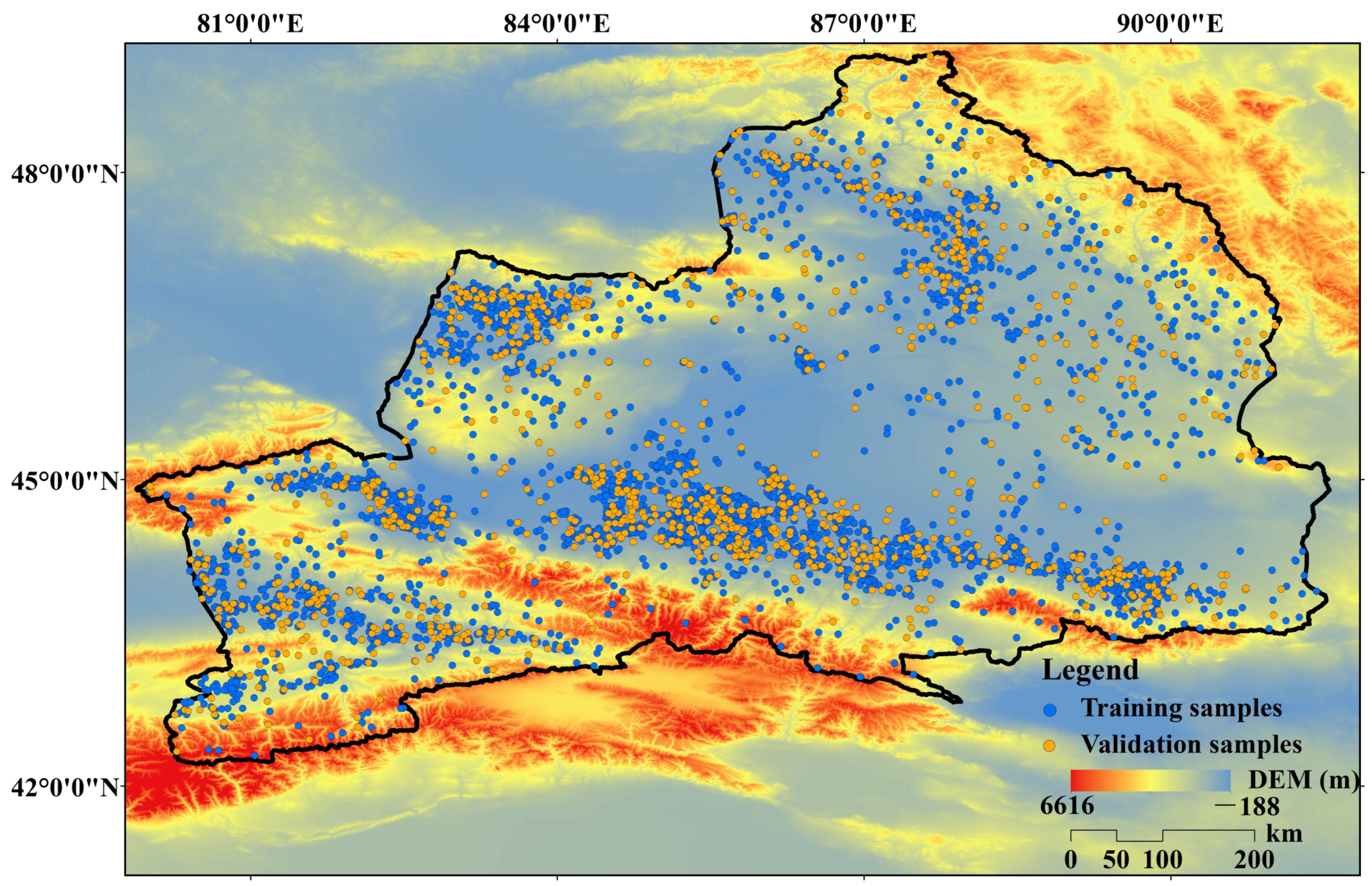
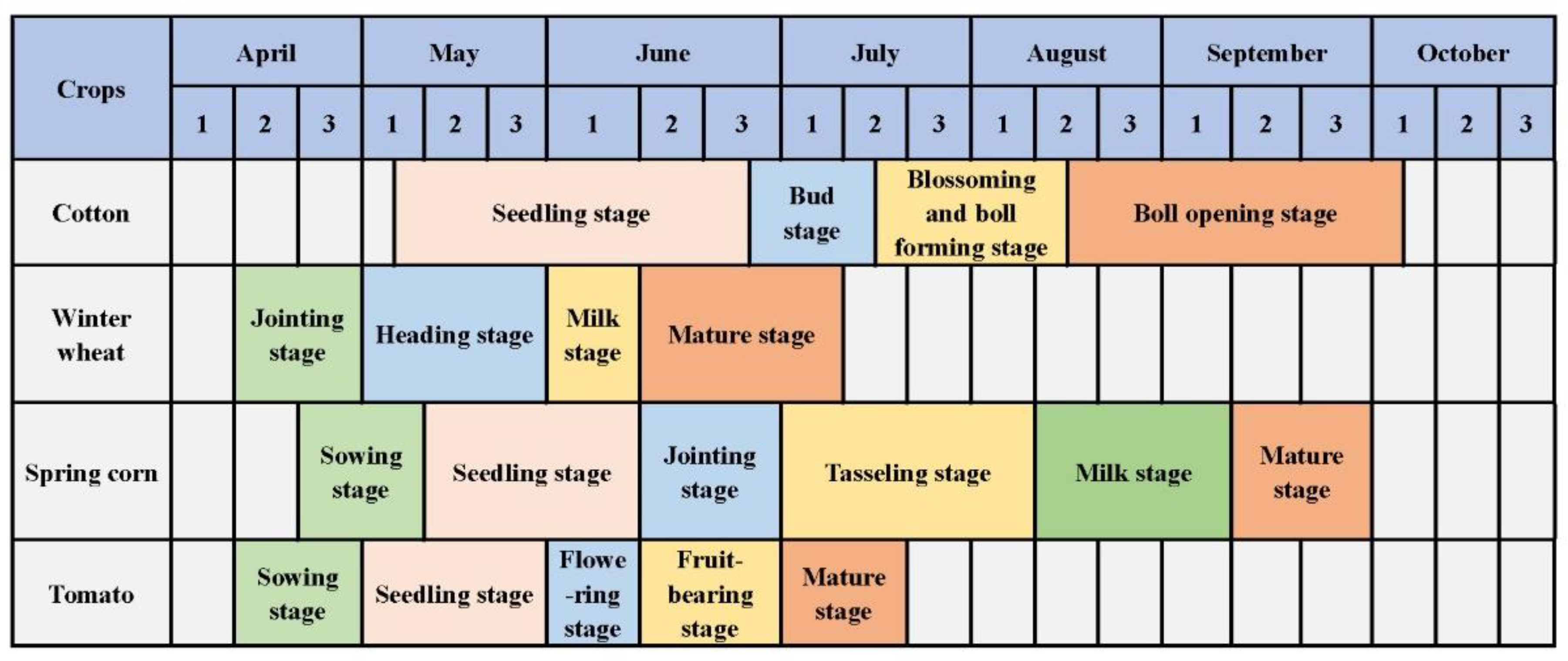
The study area was located in northern Xinjiang Province (Figure 1), which is growing large amounts of high-quality cotton. It has a temperate continental arid and semiarid climate with an annual mean temperature of −4 to 9 °C and an annual mean precipitation of 150 to 200 mm. Additionally, the frost-free season in the region is approximately 140 to 185 days. The topography in northern Xinjiang is complex and includes mountains, hills, basins, and plains. Its altitude ranges from 171 to 6616 m. Cotton in northern Xinjiang mainly has four growing stages (Figure 2): (1) seedling stage (starts in early May and ends in late June); (2) bud stage (starts in late June and ends in mid-July); (3) blossoming and boll forming stage (starts in mid-July and ends in mid-August); and (4) boll opening stage (starts in mid-August and ends in early October). In addition to cotton, tomato, corn, and wheat are also important crops planted in northern Xinjiang, and the different planting cycles of these crops provide the basis for remote sensing-based identification.
Winter wheat, spring corn, and tomato are also dominant crops in northern Xinjiang, and they have a certain common growth cycle with cotton (Figure 2). From April to July, winter wheat mainly has four growing stages, including the jointing stage (starts in middle April and ends in late April), heading stage (starts in early May and ends in late May), milk stage (starts in early June and ends in middle June), and mature stage (starts in middle June and ends in early July). Spring corn is cultivated from late April to September, mainly containing six growing stages, including the sowing stage (starts in late April and ends in early May), seedling stage (starts in middle May and ends in early June), jointing stage (starts in middle June and ends in late June), tasseling stage (starts in early July and ends in early August), milk stage (starts in middle August and ends in early September), and mature stage (starts in middle September and ends in late September). In addition, tomato mainly has five growing stages, cultivated from April to July, including the sowing stage (starts in middle April and ends in late April), seedling stage (starts in early May and ends in late May), flowering stage (starts in early June and ends in middle June), fruit-bearing stage (starts in middle June and ends in late June), and mature stage (starts in early July and ends in middle July). The differences in phenology make the certain differences in the growth of crops, which provides convenience for phenological-based algorithms to obtain better accuracy of crop extraction.
2.2. Sentinel-1 and Sentinel-2 Data
Sentinel-1 (S1) and Sentinel-2 (S2) data for 2019 were collected for this study. S1 provides data from a dual-polarized C-band Synthetic Aperture Radar (SAR) instrument with a double-star revisit period of 5 days. The main operating modes for S1 are the interference wide radiation mode and wave mode, and the homogenous subset of S1 data included the S1 Ground Range Detected (GRD) scenes. In particular, the S1 toolbox was used to generate the calibrated ortho-correction products, which helped determine the backscattering coefficient in decibels per pixel. The following preprocessing steps were used to derive the backscatter coefficient in each pixel, mainly including track file application, boundary noise removal, thermal noise removal, radiation calibration, and terrain calibration [23]. The S2 Level 2A data was also used in this study, which provided Bottom of Atmosphere reflectance images derived from the associated Level-1 C products. It is a wide-scale and high-resolution multispectral imaging mission with a 5-day revisiting period that can be used to monitor vegetation, soil, and water cover at a 10–60 m spatial resolution. The S2 top-of-atmosphere (TOA) data collected in the GEE are processed through radiometric and geometric correction. It can effectively alleviate the radiation error and geometric distortion of the image. The composition of an image is a regular method of constructing time series data, and it can reduce the influence of cloud cover and lack of observation time. The images were combined on a monthly basis. We selected the images with less than 10% cloud cover in the study period and calculated the median value of each band from the pixels for each month. It could eliminate the influence of extreme values, such as very bright or dark pixels. Finally, the composite images of S1 and S2 in May, June, July, August, and September were generated. In total, 321 S1 images and 930 S2 images were used to map cotton fields with the GEE platform (Table 1).
2.3. Identifying Cotton Fields
Figure 3 shows the framework for mapping cotton fields in northern Xinjiang. Five kinds of masks were mapped to eliminate disturbance due to non-cotton land-use types. Random sample points were generated and assessed based on the true points collected by field surveys. Specific features of the different periods were selected. Then, random forest classifiers and the multi-scale image segmentation method were combined to map the cotton fields in northern Xinjiang, and the results were verified by the measured sample points. These steps are described in detail below.
2.3.1. Calculating Vegetation Indices
The vegetation index has been widely used to qualitatively evaluate the vegetation coverage and growth, which can be used in crop monitoring. Two vegetation indices were calculated in this study: the normalized difference vegetation index (NDVI) and the enhanced vegetation index (EVI) [24,25]. These indices provide vital information about vegetation growth and biomass, respectively. In addition, the normalized difference water index (NDWI), land surface water index (LSWI), and red edge position (REP) were calculated because they have been widely used in research on water bodies, built-up areas, vegetation canopies, and other features that separately represent the mechanism underlying vegetation and other features [15,26,27]. Among them, the NDWI tends to emphasize the information on water body in the image; LSWI only needs the vegetation information at the time of measurement, and it takes into account various influencing factors such as canopy structure and observation angle, which has certain advantages in vegetation water content monitoring; and REP is highly sensitive to chlorophyll content and can monitor the growth of crops. The bands of Sentinel-1/2 and indices used in this study are shown in Table 2.
2.3.2. Mapping Non-cropland Cover Types as Masks
Mapping cotton fields at a large scale is challenging because many factors potentially affect the seasonal dynamics of vegetation indices. To reduce the potential impacts and simplify the structure of the model to reduce the workload of classification, we extracted the common land masks in northern Xinjiang using the existing threshold method and data. Therefore, some non-cotton field masks were generated.
Water body. The water bodies of northern Xinjiang are mainly concentrated in the northeast and southwest regions. The Kanas Lake, Wulungu Lake, and Aibi Lake are relatively large in area, and there are certain seasonal changes in the lakes. In order to obtain the range of all water bodies in northern Xinjiang, the NDWIs for March, July, and September were calculated to decrease the impact of seasonal changes to lakes. The Otsu method is an adaptive threshold determination method, which can maximize the between-class variance between the water body and background in the remote sensing images, to obtain the best segmentation threshold, which has been widely used in the research of water body extraction. Therefore, the Otsu method was used to determine the water body threshold as . When NDWI > , the pixel was determined to be a water body pixel. The mask was obtained by combining the results calculated above and was not included in the subsequent classification.
Built-up and barren land. There is a large area of buildings and barren land in northern Xinjiang, mainly concentrated in the central and northeastern regions, which has less precipitation throughout the year and is difficult for vegetation to grow. There are many studies that have extracted buildings and barren land through the LSWI. The whole plant growing season shown by the LSWI helped identify barren and built-up land with relatively high precision [4]. Therefore, the LSWI from March to November was calculated after taking into consideration the vegetation phenology in northern Xinjiang in this study. If the pixel values in these months were all less than 0, it was considered to be built-up or barren land.
Forest land and grassland. Forest land and grassland in northern Xinjiang are mainly concentrated in the northeast, western, and northwestern regions, while forest land and grassland in the center of northern Xinjiang are relatively few, which is dominated by barren land with sparse vegetation. Based on the 30 m resolution samples collected in 2015, the FROM-GLC 10 dataset was used to analyze the land cover map in 2017 with high overall accuracy [28]. It included crop land, forest land, grassland, etc., which meant that the forest land and grassland could be obtained based on this dataset.
2.3.3. Pixel-Based Classifier: Random Forest
The random forest classifiers are collections of classification trees, which consist of K decision trees and P random choices. It was first proposed by Breiman. When an example is classified, its variables will go to the predictor of K-tree, and K predictions will be combined by voting for the most popular category with randomness in the whole process. The random points will train each tree, and the binary problem for each node is selected from random p input variables. As a machine learning method, the random forest classifiers can effectively measure the importance of indicators and select features with high importance and rich information [29], which perform better than other models in most cases [30]. In addition, Lawrence and Moran (2015) compared the performance of various machine learning methods through consistent procedures and 30 different datasets, and found that the average classification accuracy of random forest was highest, which was significantly better than other machine learning methods, such as Support Vector Machines (SVM) [31]. Therefore, it is believed that the random forest model for cotton field extraction has better performance. In particular, the computational intensity of random forest classifiers is lower than those of other decision tree ensemble methods. They effectively integrate the variables and require minimal adjustment and supervision [32].
In this study, the composite of Sentinel-1 and Sentinel-2 data and the indices were used as classifier inputs. All the pixels outside the masks were trained and classified using random forest classifiers. Previous studies have shown that the optimal number for the decision tree is between 10 and 100 [33]. The random forest models under different decision trees were built in the study, and the overall accuracy and kappa coefficient were used as the evaluation criteria to explore the optimal number of decision trees. According to the accuracy of different models, the number of trees we selected was 21. Additionally, the number of features used in each split was set to be the square root of the number of input features, which was one of the standard settings for remote sensing [34]. The output of the classification is the value of 0 and 1, where 0 represents the pixel of non-cotton land cover and 1 represents the pixel of cotton field.
2.3.4. Object-Based Segmentation: Multi-Scale Image Segmentation
The multi-scale segmentation method, a regional growing segmentation technology, is used to recognize the boundaries of features. The information about object characteristics and relationships among classes can be fully utilized. The pixels with high homogeneity inside the object can be gathered together, which means that there are large differences between adjacent objects. Most of the segmentation methods are sensitive to noise as well as abnormal points, which slowly converge in large-scale datasets during the clustering process, such as the K-means clustering and simple non-iterative clustering methods [35,36]. The diversity of features and different scales of the objects in the remote sensing images meant that the multi-scale method was finally chosen in this study. The main parameters of the algorithm include segmentation scale and object heterogeneity index. Among them, the object heterogeneity index considers the spectral factor and shape factor, and the smoothness and refinement were further included in the shape factor. When the heterogeneity of all the segmentation control parameters reaches the minimum, the segmentation effect is best. The calculation formulas for image shape heterogeneity (Equations (1)–(3)), spectral heterogeneity (Equation (4)), and total object heterogeneity (Equation (5)) are as follows:
where is the image shape heterogeneity, represents the weight of smoothness, represents the weight of compactness, represents the heterogeneity of smoothness, represents the heterogeneity of compactness, and . Meanwhile, E represents the perimeter of the object after segmentation, B is the shortest perimeter of the circumscribed rectangle in the horizontal direction, and N is the pixel number within the quality of object.
where is the spectral heterogeneity, c represents the total number of bands, represents the weight of the band i, and represents the standard deviation of the band i.
where d is the total object heterogeneity, represents the weight of spectral heterogeneity, represents the weight of shape heterogeneity, represents the spectral heterogeneity, represents the shape heterogeneity, and .
After considering the needs of different types of ground object analyses, the best segmentation effect was obtained by adjusting the segmentation scale using the ESP 2 toolbox, which can calculate the local variance of different objects in a band and maximize homogeneity within the object [37]. The ESP 2 toolbox can be combined with multi-band images, using the cross-scale concept to automatically identify parameters to estimate the optimal scale [38], and the result was fed back using the ROC-LV line graph [39]. When the LV change rate is largest, the peak appears, and the segmentation scale is best at this time. After taking into account the spatial heterogeneity between regions, the segmentation was finally realized at the county level.
2.3.5. Combination of Pixel-Based and Object-Based Approaches
The vector boundary of the ground object was obtained based on the multi-scale segmentation method. Each vector had a unique label and was further marked as “cotton field” or “non-cotton field” patches through calculating the ratio of cotton pixels in each vector. Additionally, the threshold was used to divide cotton field and non-cotton field labels.
In detail, the rice area was extracted at a threshold of 0.6 and the built-up areas were extracted at a threshold of 0.8 [40,41]. Based on previous studies, the extraction effect of cotton fields with a threshold ranging from 0.6 to 0.8 was explored, and, finally, a threshold of 0.75 was chosen after verifying the accuracy of the cotton field maps in northern Xinjiang. That is, when the average value of the cotton field pixels in the classified patch was greater than 0.75, the patch was classified as a “cotton field”; otherwise, the patch was classified as a “non-cotton field.”
2.4. Accuracy Assessment
Accuracy assessment requires high-quality verification datasets collected at an appropriate spatial and temporal scale. Therefore, these verification datasets are an important part of the mapping process. Ground reference data for 2019 were collected using the stratified random sampling method for accuracy assessment, which was based on multiple information sources. The FROM-GLC 10 dataset was used as a basis to generate the cropland, and the cotton field and non-cotton field samples were visually selected by overlaying the random samples with the high-spatial-resolution images in Google Earth and the S2 images in 2019. Meanwhile, the true sample points were collected and the third land survey data were used as an auxiliary reference in the visual procedure. Finally, the total number of validation samples collected in this study was 947 samples, which consisted of 225 cotton field samples and 722 non-cotton field samples. These validation samples were used to calculate the confusion matrix to evaluate the accuracy. The overall accuracy (OA), producer’s accuracy (PA), user’s accuracy (UA), and kappa coefficient (k) were calculated, using the following equations:
where TP represents the actual number of cotton fields predicted as cotton fields, TN is the actual number of non-cotton fields predicted as non-cotton fields, FN is the actual number of cotton fields predicted as non-cotton fields, FP is the actual number of non-cotton fields predicted as cotton fields, represents the overall classification accuracy, and represents the ratio of the sum of the product of the number of real samples and the number of predicted samples to the square of the total number of samples.
3. Results
3.1. Key Parameter of Random Forest
As a hotspot method in the field of machine learning, random forest classifiers were widely used in the classification studies. The number of decision trees in the model is relatively dominant to the classification results. The random forest classifiers under different decision trees were constructed in this study, and the OA and kappa coefficient were used as the evaluation criteria to explore the optimal number of decision trees. The results showed that the OA and kappa coefficient of the model increased significantly when the number of the decision tree increased from 0 to 21, and remained basically unchanged after the decision tree number reached 21 (Figure 4). When the number of decision trees was 21, the OA and kappa coefficient were 0.932 and 0.813, respectively. The model ran fast and the overall efficiency was best at this time. It indicated that the number of decision trees could effectively improve the accuracy of the model, but the accuracy would not change significantly as the number of decision trees exceeded 21 in this study. When exceeding the threshold, the model will become redundant, resulting in a slower training speed and lower efficiency of the classification process.
3.2. Spatial Distribution of Cotton Fileds
The 10 m distribution map for cotton fields in northern Xinjiang in 2019 was finally obtained based on random forest classifiers and the multi-scale image segmentation method, combined with S1 and S2 data for the five months. Accuracy assessments of the resultant cotton field map were conducted using the validation samples, and the results indicated that the extracted cotton field map in this study was highly accurate, with an OA, PA, UA, and kappa coefficient of 0.932, 0.846, 0.871, and 0.813, respectively.
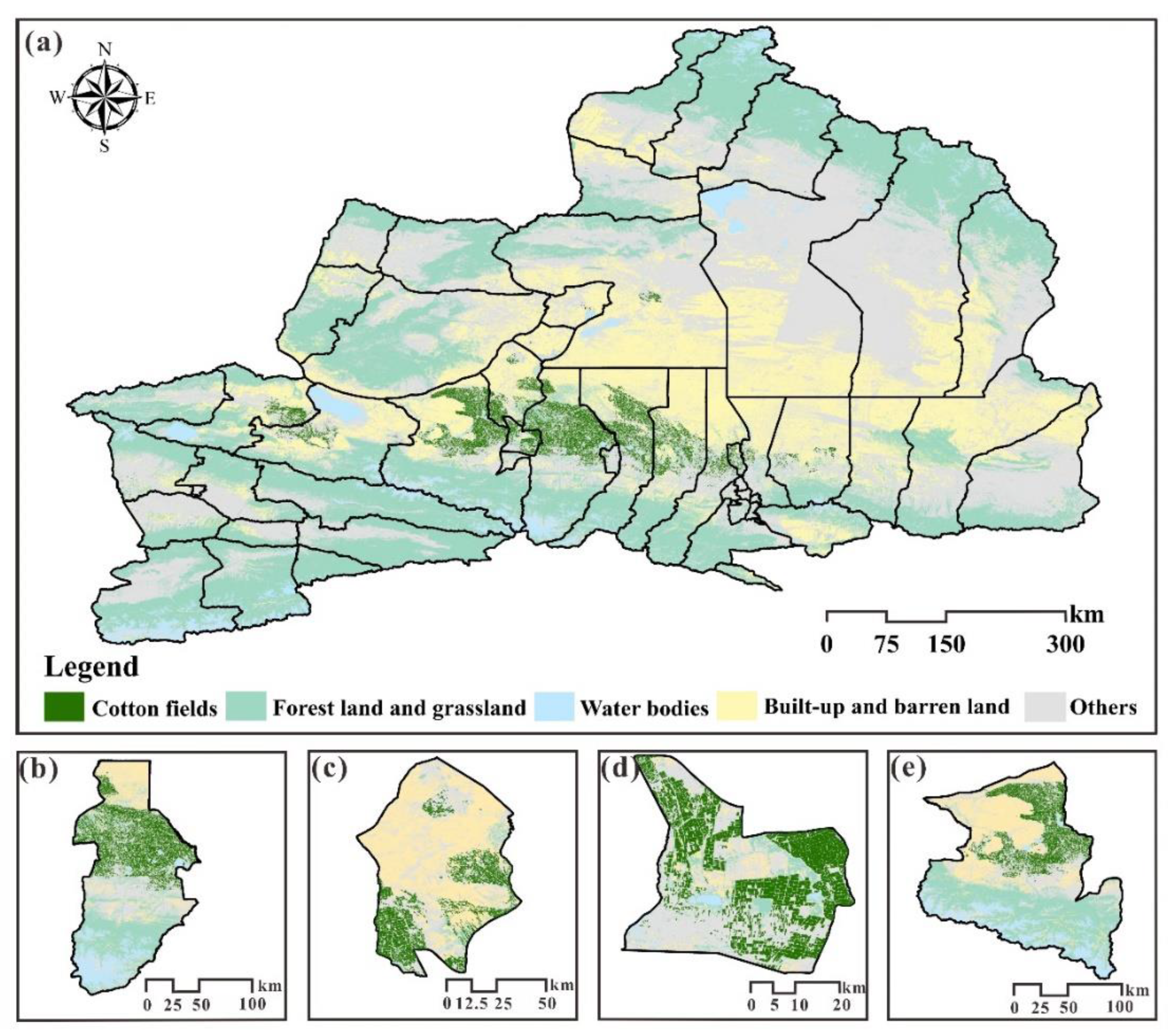
The results showed that the total area of cotton fields in northern Xinjiang in 2019 was 8.66 103 km2 (Figure 5). Cotton fields were mainly distributed in 15 out of 34 counties (with area of cotton fields larger than 10 km2), and the two counties with the largest area of cotton fields were Shawan County and Wusu City, with planting areas of 2.36 103 km2 and 1.76 103 km2, respectively. The cotton field planting areas in Huocheng County and Shihezi City were relatively small (15.7 km2 and 36.0 km2, respectively). The spatial distribution characteristics of the cotton fields showed that they were mainly concentrated in the central part of northern Xinjiang and the plains north of the Tianshan Mountains. There was a continuous distribution of large cotton fields, mainly in Shawan County (2.36 103 km2), Wusu City (1.76 103 km2), Manasi County (1.30 103 km2), Hutubi County (8.71 102 km2), and Karamay District (6.27 102 km2). However, compared to the other crops, the cotton fields planting area in the north of northern Xinjiang was relatively small because the main crop was winter wheat.
3.3. Optimal Phenological Phase
It was difficult to obtain the remote sensing data during the critical periods of the crop growing season because they were frequently affected by the cloud cover. This study focused on exploring the optimal month for mapping cotton fields, which could be used to simplify the work of crop classification by filtering the crop phenological phases. The cotton fields were extracted based on single-phase data from May to September and the combined data from different phases. The results showed that in the case of single-phase data extraction, mapping cotton fields based on the data in August was highly accurate, with the highest OA and kappa coefficient of 0.921 and 0.783, respectively (Table 3). The cotton characteristics were quite different from other crops in mid-to-late August because it was in the boll opening stage. The accuracy of the cotton field map based on the data in May was lowest, with the OA and kappa coefficient of 0.838 and 0.532, respectively (Table 3). At that time, the cotton was at the seedling stage, which was similar to the characteristics of other crops in the same growth period, such as corn.
The results for the multi-phase data extraction of the cotton fields showed that combining the images in June and August could achieve better accuracy, with an OA and kappa coefficient of 0.925 and 0.792, respectively. In both months, the cotton was in the late seedling stage and the early boll opening stage, respectively, making the remote sensing characteristics of cotton fields and other crops quite different. Furthermore, the area of cotton fields extracted based on remote sensing images in June and August was 8.65 103 km2 with less than 1% error compared to the area of cotton fields extracted based on the whole growth period. Therefore, based on the multi-phase data in June and August, the classification method could effectively reduce feature redundancy in the cotton field extraction process and the image processing workload, which would improve the efficiency of cotton field extraction. In this case, the high-precision identification of cotton fields could be achieved during the boll opening period (August). Cotton harvesting in northern Xinjiang was concentrated in early-to-mid October, and thus the mapping work could be completed about 40 days before the harvest. This would provide timely and accurate decisions supporting the spatial allocation of labor for cotton harvesting.
4. Discussion
4.1. Key Classification Features
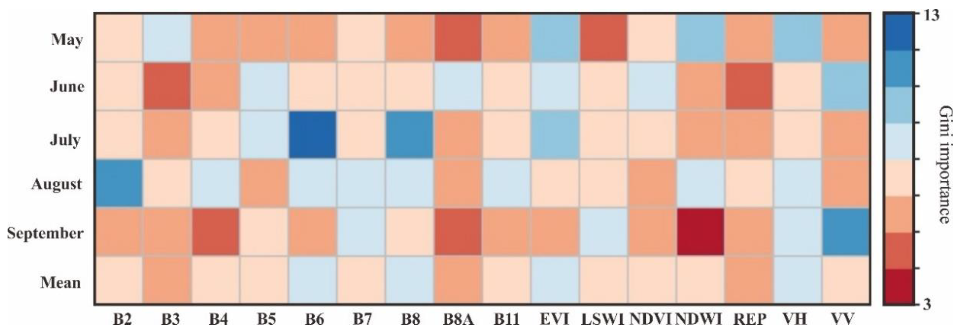
The variable importance of each index can be obtained based on the random forest classifiers, and then the contribution of different features to the model can be determined [42]. It was found that the EVI and the red edge bands (especially band 6) were the most important predictors in the cotton fields extraction process, with the EVI ranked second (Figure 6). Furthermore, it has also been used in previous studies on land surface coverage classification to produce high-precision land use/cover maps, such as shrubs, rice fields, and soybean fields [43,44,45]. Meanwhile, S2 band 6 (RE2) was the most important band in the red edge bands and its importance for crop classification was also confirmed by Radoux et al. (2016) [46]. However, Forkuor et al. (2017) found that S2 band 5 (RE1) performed better than RE2 and S2 band 7 (RE3) [47], which was the opposite of our results. The contrary differences in these results may be caused by the different crops that were focused on in the studies. Furthermore, the contribution made by S2 band 11 (SWIR) was not obvious in the crop classification, and Immitzer et al. (2016) also confirmed its weak contribution in the classification of some crops, although it played an important role in farmland extraction [48,49].
As for the SAR data, the contributions made by VH and VV polarization were both high in the extraction of cotton fields. The SAR data was sensitive to the geometric characteristics of the observed object, which could help distinguish the different categories of specific ground objects [14]. For example, the built-up area appeared bright in the radar image due to its double bounce scattering characteristic, while roads often appeared dark due to their smooth surface [50]. The vegetation cover, leaf size, water content, and height characteristics varied differently during the growth cycle stages of cotton, which affected the scattering mechanism and corresponding scattering intensity of the SAR data [51]. The high vegetation coverage and leaf density during the cotton bud stage, as well as the blossoming and boll forming stage, meant that the vegetation canopy could not be penetrated by C-band radar waves. Therefore, volume and surface scattering were the main influencing factors, and the contributions made by VV and VH polarization were limited, especially compared with the boll opening stage. The cotton was in the boll opening stage in mid-to-late September and the leaves were beginning to decay. Therefore, the vegetation canopy was penetrated by the C-band radar and echo scattering occurred through the cotton stalks, which meant that the contributions made by VH and VV polarization reached a peak. Therefore, it was a promising method to detect the cotton fluffing period based on SAR data.
The results also showed that the cotton fields could be effectively identified based on the images obtained from a designated phenological phase. Additionally, combining multi-source Sentinel data increased the visit time and improved the spatial resolution of the data usually applied in crop extraction [52]. Based on the combination of S1 and S2 data, a cotton field map at a higher resolution could be drawn within a certain phenological phase. Converting “whole growing stage” extraction into “specific phenological phase” extraction greatly simplifies the extraction work of cotton fields [53], and it could overcome problems associated with cloud cover in some periods of some areas. In particular, the phenological extraction algorithm based on S1 and S2 data could provide more detailed spatial information than the MODIS and Landsat images-based ones because there are fewer mixed pixels in the Sentinel data. With the free provision of Sentinel data, it could eventually support real-time crop monitoring in the future. The extraction method using a single-period phenological feature index based on S1 and S2 data would improve the ability to map and characterize cotton fields and could be applied to the extraction of other crops.
4.2. Appilications and Limitations
High-resolution crop mapping over large areas is a major challenge in agricultural remote sensing [54]. The single satellite sensor has inherent observation limitations, which is the main reason for the current low accuracy of crop monitoring [55]. Therefore, in view of the shortcomings of the single satellite data source, it should be further strengthened for the collaborative inversion of different data sources, especially through combining optical remote sensing with radar and other sensors to generate high-quality crop monitoring data products in the future [56].
Meanwhile, it is also needed to focus on the defects and requirements in the existing methods of crop monitoring. In previous studies, it was difficult to obtain high-resolution remote sensing images, the process of dealing with a large number of images was complicated, and the cost of large-scale cotton field mapping was relatively high. Now, the platforms such as GEE have partly solved the shortcomings of a few working groups with powerful computing capability, which is necessary for large-scale and high-resolution crop mapping [57,58].
Besides, the remote sensing image is often affected by various factors such as cloud cover, making it difficult to find a suitable one in a certain area. Combining the S1 and S2 data can greatly reduce the influence of the factors, such as their behaving in cotton field mapping in this study. It was also proved that the combination of S1 and S2 had great feasibility and reliability for cotton field mapping in northern Xinjiang. Moreover, the combination of random forest and multi-scale image segmentation was used to extract cotton fields, which provided a new approach for crop mapping. Compared with the traditional methods, this approach can reduce the influence of noise generated in the mapping process [59]. It was proposed that cotton field mapping could be accurately achieved about 40 days before harvest, which was of great significance for agricultural system management [53]. Based on the information of crop extraction in different periods, we can accurately identify its spatial distribution in time. The early realization of crop identification can help with decision making related to crop management and the associated disaster warning. For example, local government can respond fast to certain disasters, such as developing harvesting plans [60].
Furthermore, some potential sources of uncertainty affecting the mapping results still exist. The FROM-GLC 10 dataset was used in this study to eliminate interference by forest land and grassland, although the dataset had its limitations, such as the classification error [61]. Additionally, the complexity of the region could cause uncertainty about the threshold for fusing the pixel-based and object-based methods. Therefore, the threshold needs to be adjusted when applied to different regions. Meanwhile, mapping cotton fields was only applied to northern Xinjiang in 2019 in this study. In addition, different methods should be applied and compared to verify the specific performance of the method proposed in this study. That is to say, far more extensive studies should be conducted in cotton field mapping using different methods, expanding the range of the study area, and increasing the time range.
5. Conclusions
Obtaining the planting area and spatial distribution of cotton fields is essential for timely and accurate agricultural management in northern Xinjiang. However, there is currently no suitable large-scale and high-resolution cotton field monitoring method, and the timing and important characteristics of cotton fields are not clear. Therefore, a new framework for mapping cotton fields was developed in this study. It used optical and SAR data for different phenological periods, and random forest classifiers and the multi-scale image segmentation method were combined to extract the cotton fields. It can reduce the interference of cloud cover and make less noise in the extraction process, providing an effective approach for high-resolution and high-precision cotton field mapping. Using the proposed framework, we generated a cotton field map for northern Xinjiang in 2019 at a spatial resolution of 10 m. The results showed that S1 and the red edge bands in S-2 were most important for mapping cotton fields, and the fusion of optical images and microwave images for crop mapping showed great potential. Meanwhile, the boll opening stage was the best phenological phase for mapping cotton fields, which was about 40 days before harvest, and thus, local government would have enough time to make harvesting labor allocation decisions. The proposed new framework has great potential to be applied in the mapping and monitoring of other crops.
Author Contributions
T.H., Y.H. and J.P. designed the study. T.H. and J.P. made significant contributions to analyze and interpret the data; T.H. and Y.H. finished the first manuscript. Y.H., J.D. and S.Q. reviewed and approved the manuscript. All authors have read and agreed to the published version of the manuscript.
Funding
This research was funded by the National Key Research and Development Program of China, grant number 2017YFA0604704.
Institutional Review Board Statement
Not applicable.
Informed Consent Statement
Not applicable.
Data Availability Statement
The Sentinel-1 and Sentinel-2 datasets were offered by the European Space Agency. The FROM-GLC data are available through Finer Resolution Observation and Monitoring—Global Land Cover (http://0-data-ess-tsinghua-edu-cn.brum.beds.ac.uk/, accessed on 21 October 2020).
Acknowledgments
The authors are grateful to the editors and reviewers for reviewing the manuscript.
Conflicts of Interest
The authors declare no conflict of interest.
References
- King, L.; Adusei, B.; Stehman, S.V.; Potapov, P.V.; Song, X.P.; Krylov, A.; Di Bella, C.; Loveland, T.R.; Johnson, D.M.; Hansen, M.C. A multi-resolution approach to national-scale cultivated area estimation of soybean. Remote Sens. Environ. 2017, 195, 13–29. [Google Scholar] [CrossRef]
- Xiao, X.; Boles, S.; Liu, J.Y.; Zhuang, D.F.; Frolking, S.; Li, C.S.; Salas, W.; Moore, B. Mapping paddy rice agriculture in southern China using multi-temporal MODIS images. Remote Sens. Environ. 2005, 95, 480–492. [Google Scholar] [CrossRef]
- Wang, J.; Xiao, X.M.; Liu, L.; Wu, X.C.; Qin, Y.W.; Steiner, J.L.; Dong, J.W. Mapping sugarcane plantation dynamics in Guangxi, China, by time series Sentinel-1, Sentinel-2 and Landsat images. Remote Sens. Environ. 2020, 247, 111951. [Google Scholar] [CrossRef]
- Qin, Y.; Xiao, X.M.; Dong, J.W.; Zhou, Y.T.; Zhou, Z.; Zhang, G.L.; Du, G.M.; Jin, C.; Kou, W.L.; Wang, J.; et al. Mapping paddy rice planting area in cold temperate climate region through analysis of time series Landsat 8 (OLI), Landsat 7 (ETM+) and MODIS imagery. ISPRS J. Photogramm. Remote Sens. 2015, 105, 220–233. [Google Scholar] [CrossRef] [Green Version]
- Liu, Z.H.; Yang, P.; Tang, H.J.; Wu, W.B.; Zhang, L.; Yu, Q.Y.; Li, Z.G. Shifts in the extent and location of rice cropping areas match the climate change pattern in China during 1980–2010. Reg. Environ. Chang. 2015, 15, 919–929. [Google Scholar] [CrossRef]
- Hao, P.Y.; Tang, H.J.; Chen, Z.X.; Meng, Q.Y.; Kang, Y.P. Early-season crop type mapping using 30-m reference time series. J. Integr. Agric. 2020, 19, 1897–1911. [Google Scholar] [CrossRef]
- Hao, P.Y.; Zhan, Y.L.; Wang, L.; Niu, Z.; Shakir, M. Feature selection of time series MODIS data for early crop classification using Random Forest: A case study in Kansas, USA. Remote Sens. 2015, 7, 5347–5369. [Google Scholar] [CrossRef] [Green Version]
- Bridhikitti, A.; Overcamp, T. Estimation of Southeast Asian rice paddy areas with different ecosystems from moderate-resolution satellite imagery. Agric. Ecosyst. Environ. 2012, 146, 113–120. [Google Scholar] [CrossRef]
- Chen, B.; Jin, Y.F.; Brown, P. Automatic mapping of planting year for tree crops with Landsat satellite time series stacks. ISPRS J. Photogramm. Remote Sens. 2019, 151, 176–188. [Google Scholar] [CrossRef]
- Wang, Z.L.; Lai, C.G.; Chen, X.H.; Yang, B.; Zhao, S.W.; Bai, X.Y. Flood hazard risk assessment model based on Random Forest. Water Resour. Res. 2015, 527, 1130–1141. [Google Scholar] [CrossRef]
- Jin, Z.N.; Azzari, G.; You, C.; di Tommaso, S.; Aston, S.; Burke, M.; Lobell, D.B. Smallholder maize area and yield mapping at national scales with Google Earth Engine. Remote Sens. Environ. 2019, 228, 115–128. [Google Scholar] [CrossRef]
- Son, N.T.; Chen, C.F.; Chen, C.R.; Toscano, P.; Cheng, Y.S.; Guo, H.Y.; Syu, C.H. A phenological object-based approach for rice crop classification using time-series Sentinel-1 Synthetic Aperture Radar (SAR) data in Taiwan. Int. J. Remote Sens. 2021, 42, 2722–2739. [Google Scholar] [CrossRef]
- Yang, H.J.; Pan, B.; Li, N.; Wang, W.; Zhang, J.; Zhang, X.L. A systematic method for spatio-temporal phenology estimation of paddy rice using time series Sentinel-1 images. Remote Sens. Environ. 2021, 259, 112394. [Google Scholar] [CrossRef]
- Gasparovic, M.; Klobucar, D. Mapping floods in lowland forest using Sentinel-1 and Sentinel-2 data and an object-based approach. Forests 2021, 12, 553. [Google Scholar] [CrossRef]
- Xiong, J.; Thenkabail, P.S.; Gumma, M.K.; Teluguntla, P.; Poehnelt, J.; Congalton, R.G.; Yadav, K.; Thau, D. Automated cropland mapping of continental Africa using Google Earth Engine cloud computing. ISPRS J. Photogramm. Remote Sens. 2017, 126, 225–244. [Google Scholar] [CrossRef] [Green Version]
- Hu, Q.; Wu, W.B.; Xia, T.; Yu, Q.Y.; Yang, P.; Li, Z.G.; Song, Q. Exploring the use of google earth imagery and object-based methods in land use/cover mapping. Remote Sens. 2013, 5, 6026–6042. [Google Scholar] [CrossRef] [Green Version]
- Zhou, W.Q.; Troy, A.; Grove, M. Object-based land cover classification and change analysis in the Baltimore metropolitan area using multitemporal high resolution remote sensing data. Sensors 2008, 8, 1613–1636. [Google Scholar] [CrossRef] [PubMed] [Green Version]
- Zhong, L.H.; Gong, P.; Biging, G.S. Efficient corn and soybean mapping with temporal extendability: A multi-year experiment using Landsat imagery. Remote Sens. Environ. 2014, 140, 1–13. [Google Scholar] [CrossRef]
- Liu, Z.H.; Hu, Q.; Tan, J.Y.; Zou, J.Q. Regional scale mapping of fractional rice cropping change using a phenology-based temporal mixture analysis. Int. J. Remote Sens. 2019, 40, 2703–2716. [Google Scholar] [CrossRef]
- Werner, J.P.S.; Oliveira, S.R.D.; Esquerdo, J.C.D.M. Mapping cotton fields using data mining and MODIS time-series. Int. J. Remote Sens. 2019, 41, 2457–2476. [Google Scholar] [CrossRef]
- Wu, W.B.; Yang, P.; Tang, H.J.; Zhou, Q.B.; Chen, Z.X.; Shibasaki, R. Characterizing spatial patterns of phenology in cropland of China based on remotely sensed data. Agric. Sci. China 2010, 9, 101–112. [Google Scholar] [CrossRef]
- Gorelick, N.; Hancher, M.; Dixon, M.; Ilyushchenko, S.; Thau, D.; Moore, R. Google Earth Engine: Planetary-scale geospatial analysis for everyone. Remote Sens. Environ. 2017, 202, 18–27. [Google Scholar] [CrossRef]
- Minasny, B.; Shah, R.M.; Che Soh, N.; Arif, C.; Indra Setiawan, B. Automated near-real-time mapping and monitoring of rice extent, cropping patterns, and growth stages in Southeast Asia using Sentinel-1 time series on a Google Earth Engine platform. Remote Sen. 2019, 11, 1666. [Google Scholar] [CrossRef] [Green Version]
- Fung, T.; Siu, W. Environmental quality and its changes, an analysis using NDVI. Int. J. Remote Sens. 2000, 21, 1011–1024. [Google Scholar] [CrossRef]
- Huete, A.; Didan, K.; Miura, T.; Rodriguez, E.P.; Gao, X.; Ferreira, L.G. Overview of the radiometric and biophysical performance of the MODIS vegetation indices. Remote Sens. Environ. 2002, 83, 195–213. [Google Scholar] [CrossRef]
- Gao, B.C. NDWI—A normal difference water index for remote sensing of vegetation liquid water from space. Remote Sens. Environ. 1996, 58, 257–266. [Google Scholar] [CrossRef]
- Dash, J.; Curran, P.J. The MERIS terrestrial chlorophyll index. Int. J. Remote Sens. 2004, 25, 5403–5413. [Google Scholar] [CrossRef]
- Gong, P.; Liu, H.; Zhang, M.N.; Li, C.C.; Wang, J.; Huang, H.B.; Clinton, N.; Ji, L.Y.; Li, W.Y.; Bai, Y.Q.; et al. Stable classification with limited sample: Transferring a 30-m resolution sample set collected in 2015 to mapping 10-m resolution global land cover in 2017. Sci. Bull. 2019, 64, 370–373. [Google Scholar] [CrossRef] [Green Version]
- Georganos, S.; Grippa, T.; Vanhuysse, S.; Lennert, M.; Shimoni, M.; Kalogirou, S.; Wolff, E. Less is more: Optimizing classification performance through feature selection in a very-high-resolution remote sensing object-based urban application. GISci. Remote Sens. 2018, 55, 221–242. [Google Scholar] [CrossRef]
- Goldblatt, R.; Stuhlmacher, M.F.; Tellman, B.; Clinton, N.; Hanson, G.; Georgescu, M.; Wang, C.Y.; Serrano-Candela, F.; Khandelwal, A.K.; Cheng, W.H.; et al. Using Landsat and nighttime lights for supervised pixel-based image classification of urban land cover. Remote Sens. Environ. 2018, 205, 253–275. [Google Scholar] [CrossRef]
- Lawrence, R.L.; Moran, C.J. The America View classification methods accuracy comparison project: A rigorous approach for model selection. Remote Sens. Environ. 2015, 17, 115–120. [Google Scholar] [CrossRef]
- Stevens, F.R.; Gaughan, A.E.; Linard, C.; Tatem, A.J. Disaggregating census data for population mapping using Random Forests with remotely-sensed and ancillary data. PLoS ONE 2015, 10, e0107042. [Google Scholar] [CrossRef] [Green Version]
- Rodriguez-Galiano, V.F.; Ghimire, B.; Rogan, J.; Chica-Olmo, M.; Rigol-Sanchez, J.P. An assessment of the effectiveness of a Random Forest classifier for land-cover classification. ISPRS J. Photogramm. Remote Sens. 2012, 67, 93–104. [Google Scholar] [CrossRef]
- Singha, M.; Dong, J.; Zhang, G.; Xiao, X. High resolution paddy rice maps in cloud-prone Bangladesh and Northeast India using Sentinel-1 data. Sci. Data. 2019, 6. [Google Scholar] [CrossRef]
- Wang, Y.J.; Qi, Q.W.; Liu, Y.; Jiang, L.L.; Wang, J. Unsupervised segmentation parameter selection using the local spatial statistics for remote sensing image segmentation. Int. J. Appl. Earth Obs. Geoinf. 2019, 81, 98–109. [Google Scholar] [CrossRef]
- Su, T.F.; Zhang, S.W. Local and global evaluation for remote sensing image segmentation. ISPRS J. Photogramm. Remote Sens. 2017, 130, 256–276. [Google Scholar] [CrossRef]
- Dragut, L.; Csillik, O.; Eisank, C.; Tiede, D. Automated parameterization for multi-scale image segmentation on multiple layers. ISPRS J. Photogramm. Remote Sens. 2014, 88, 119–127. [Google Scholar] [CrossRef] [Green Version]
- Dragut, L.; Tiede, D.; Levick, S.R. ESP: A tool to estimate scale parameter for multiresolution image segmentation of remotely sensed data. Int. J. Geogr. Inf. Sci. 2010, 24, 859–871. [Google Scholar] [CrossRef]
- Woodcock, C.; Strahler, A. The factor of scale in remote sensing. Remote Sens. Environ. 1987, 21, 311–332. [Google Scholar] [CrossRef]
- Ma, X.L.; Tong, X.H.; Liu, S.C.; Luo, X.; Xie, H.; Li, C.M. Optimized sample selection in SVM classification by combining with DMSP-OLS, Landsat NDVI and GlobeLand30 products for extracting urban built-up areas. Remote Sens. 2017, 9, 236. [Google Scholar] [CrossRef] [Green Version]
- Zhang, X.; Wu, B.F.; Ponce-Campos, G.E.; Zhang, M.; Chang, S.; Tian, F.Y. Mapping up-to-date paddy rice extent at 10 m resolution in China through the integration of optical and synthetic aperture radar images. Remote Sens. 2018, 10, 1200. [Google Scholar] [CrossRef] [Green Version]
- Chan, J.C.W.; Paelinckx, D. Evaluation of Random Forest and adaboost tree-based ensemble classification and spectral band selection for ecotope mapping using airborne hyperspectral imagery. Remote Sens. Environ. 2008, 112, 2999–3011. [Google Scholar] [CrossRef]
- Pan, Y.Z.; Li, L.; Zhang, J.S.; Liang, S.L.; Zhu, X.F.; Sulla-Menashe, D. Winter wheat area estimation from MODIS-EVI time series data using the Crop Proportion Phenology Index. Remote Sens. Environ. 2012, 119, 232–242. [Google Scholar] [CrossRef]
- Chen, B.Q.; Li, X.P.; Xiao, X.M.; Zhao, B.; Dong, J.W.; Kou, W.L.; Qin, Y.W.; Yang, C.; Wu, Z.X.; Sun, R.; et al. Mapping tropical forests and deciduous rubber plantations in Hainan Island, China by integrating PALSAR 25-m and multi-temporal Landsat images. Int. J. Appl. Earth Obs. Geoinf. 2016, 50, 117–130. [Google Scholar] [CrossRef]
- Grzegozewski, D.M.; Johann, J.A.; Uribe-Opazo, M.A.; Mercante, E.; Coutinho, A.C. Mapping soya bean and corn crops in the State of Parana, Brazil, using EVI images from the MODIS sensor. Int. J. Remote Sens. 2016, 37, 1257–1275. [Google Scholar] [CrossRef]
- Radoux, J.; Chome, G.; Jacques, D.C.; Waldner, F.; Bellemans, N.; Matton, N.; Lamarche, C.; d’Andrimont, R.; Defourny, P. Sentinel-2’s potential for sub-pixel landscape feature detection. Remote Sens. 2016, 8, 488. [Google Scholar] [CrossRef] [Green Version]
- Forkuor, G.; Dimobe, K.; Serme, I.; Tondoh, J.E. Landsat-8 vs. Sentinel-2: Examining the added value of sentinel-2’s red-edge bands to land-use and land-cover mapping in Burkina Faso. GISci. Remote Sens. 2017, 55, 331–354. [Google Scholar] [CrossRef]
- Immitzer, M.; Vuolo, F.; Atzberger, C. First experience with Sentinel-2 data for crop and tree species classification in central Europe. Remote Sen. 2016, 8, 166. [Google Scholar] [CrossRef]
- Vogelmann, J.E.; Tolk, B.; Zhu, Z.L. Monitoring orest changes in the southwestern United States using multitemporal Landsat data. Remote Sens. Environ. 2009, 113, 1739–1748. [Google Scholar] [CrossRef]
- Blasco, J.M.D.; Fitrzyk, M.; Patruno, J.; Ruiz-Armenteros, A.M.; Marconcini, M. Effects on the double bounce detection in urban areas based on SAR polarimetric characteristics. Remote Sens. 2020, 12, 1187. [Google Scholar] [CrossRef] [Green Version]
- Gella, G.W.; Bijker, W.; Belgiu, M. Mapping crop types in complex farming areas using SAR imagery with dynamic time warping. ISPRS J. Photogramm. Remote Sens. 2021, 175, 171–183. [Google Scholar] [CrossRef]
- Steinhausen, M.J.; Wagner, P.D.; Narasimhan, B.; Waske, B. Combining Sentinel-1 and Sentinel-2 data for improved land use and land cover mapping of monsoon regions. Int. J. Appl. Earth Obs. Geoinf. 2018, 73, 595–604. [Google Scholar] [CrossRef]
- Dong, J.W.; Xiao, X.M.; Menarguez, M.A.; Zhang, G.L.; Qin, Y.W.; Thau, D.; Biradar, C.; Moore, B. Mapping paddy rice planting area in northeastern Asia with Landsat 8 images, phenology-based algorithm and Google Earth Engine. Remote Sens. Environ. 2016, 185, 142–154. [Google Scholar] [CrossRef] [PubMed] [Green Version]
- You, N.S.; Dong, J.W. Examining earliest identifiable timing of crops using all available Sentinel 1/2 imagery and Google Earth Engine. ISPRS J. Photogramm. Remote Sens. 2020, 161, 109–123. [Google Scholar] [CrossRef]
- Illera, P.; Delgado, A.J.; Calle, A. A navigation algorithm for satellite images. Int. J. Remote Sens. 1996, 17, 577–588. [Google Scholar] [CrossRef]
- Ryu, Y.; Berry, J.A.; Baldocchi, D.D. What is global photosynthesis? History, uncertainties and opportunities. Remote Sens. Environ. 2019, 223, 95–114. [Google Scholar] [CrossRef]
- Shelestov, A.; Lavreniuk, M.; Kussul, N.; Novikov, A.; Skakun, S. Exploring Google Earth Engine platform for big data processing: Classification of multi-temporal satellite imagery for crop mapping. Front. Earth Sci. 2017, 5, 1–10. [Google Scholar] [CrossRef] [Green Version]
- Tamiminia, H.; Salehi, B.; Mahdianpari, M.; Quackebush, L.; Adeli, S.; Brisco, B. Google Earth Engine for geo-big data applications: A meta-analysis and systematic review. ISPRS J. Photogramm. Remote Sens. 2020, 164, 152–170. [Google Scholar] [CrossRef]
- Deines, J.M.; Kendall, A.D.; Crowley, M.A.; Rapp, J.; Cardille, J.A.; Hyndman, D.W. Mapping three decades of annual irrigation across the US High Plains Aquifer using Landsat and Google Earth Engine. Remote Sens. Environ. 2019, 233, 111400. [Google Scholar] [CrossRef]
- Defourny, P.; Bontemps, S.; Bellemans, N.; Cara, C.; Dedieu, G.; Guzzonato, E.; Hagolle, O.; Inglada, J.; Nicola, L.; Rabaute, T.; et al. Near real-time agriculture monitoring at national scale at parcel resolution: Performance assessment of the Sen2-Agri automated system in various cropping systems around the world. Remote Sens. Environ. 2019, 221, 551–568. [Google Scholar] [CrossRef]
- Phalke, A.R.; Ozdogan, M.; Thenkabail, P.S.; Erickson, T.; Gorelick, N.; Yadav, K.; Congalton, R.G. Mapping croplands of Europe, Middle East, Russia, and Central Asia using Landsat, Random Forest, and Google Earth Engine. ISPRS J. Photogramm. Remote Sens. 2020, 167, 104–122. [Google Scholar] [CrossRef]
Figure 1.
Geographical location and ground samples of northern Xinjiang, China.

Figure 2.
Phenology calendars for the major crops in northern Xinjiang in 2019.

Figure 3.
Framework for mapping cotton fields.

Figure 4.
Relationship between the number of decision trees and the overall accuracy, as well as kappa coefficient.
Figure 4.
Relationship between the number of decision trees and the overall accuracy, as well as kappa coefficient.

Figure 5.
Spatial distribution of cotton fields in northern Xinjiang (a). Some major cotton planting areas are shown in (b) Shawan County, (c) Karamay District, (d) Kuitun City, and (e) Wusu City.
Figure 5.
Spatial distribution of cotton fields in northern Xinjiang (a). Some major cotton planting areas are shown in (b) Shawan County, (c) Karamay District, (d) Kuitun City, and (e) Wusu City.

Figure 6.
Gini importance contrast of different classification features in each month.


Table 1.
Summary of the S1 and S2 images in this study.
| Sensor | Resolution (m) | Revisit (Days) | Scenes | ||||
|---|---|---|---|---|---|---|---|
| May | Jun. | Jul. | Aug. | Sep. | |||
| Sentinel-2 | 10/20 | 5 | 149 | 161 | 214 | 223 | 183 |
| Sentinel-1 | 10 | 12 | 73 | 56 | 61 | 65 | 66 |
Table 2.
Bands of Sentinel-1 and Sentinel-2 data and the indices used in this study.
| Sensor | Spectral Band | Wavelength (Micron) | Resolution(m) |
|---|---|---|---|
| Sentinel-1 | VH | 10 | |
| VV | 10 | ||
| Sentinel-2 | Band 2—Blue | 496.6 (S2A)/492.1 (S2B) | 10 |
| Band 3—Green | 560.0 (S2A)/559.0 (S2B) | 10 | |
| Band 4—Red | 664.5 (S2A)/665.0 (S2B) | 10 | |
| Band 5—Red Edge 1 | 703.9 (S2A)/703.8 (S2B) | 20 | |
| Band 6—Red Edge 2 | 740.2 (S2A)/739.1 (S2B) | 20 | |
| Band 7—Red Edge 3 | 782.5 (S2A)/779.7 (S2B) | 20 | |
| Band 8—NIR | 835.1 (S2A)/833.0 (S2B) | 10 | |
| Band 8A—Red Edge 4 | 864.8 (S2A)/864.0 (S2B) | 20 | |
| Band 11—SWIR 1 | 1613.7 (S2A)/1610.4 (S2B) | 20 | |
| NDVI = (Band 8 − Band 4)/(Band8 + Band 4) | 10 | ||
| EVI = 2.5 × (Band 8 − Band 4)/(Band 8 + 6 × Band 4 − 7.5 × Band 2 +1) | 10 | ||
| NDWI = (Band 3 − Band 8)/(Band 3 + Band 8) | 10 | ||
| LSWI = (Band 8 − Band 11)/(Band 8 + Band 11) | 10 | ||
| REP = 705 + 35 × (0.5 × (Band 7 + Band 4) − Band 5)/(Band 6 − Band 5) | 10 |
Table 3.
Accuracy of the cotton field extraction with different phases.
| Month | Overall Accuracy | User’s Accuracy | Producer’s Accuracy | Kappa Coefficient |
|---|---|---|---|---|
| May | 0.838 | 0.685 | 0.591 | 0.532 |
| Jun. | 0.914 | 0.824 | 0.813 | 0.763 |
| Jul. | 0.902 | 0.797 | 0.787 | 0.728 |
| Aug. | 0.921 | 0.826 | 0.844 | 0.783 |
| Sep. | 0.899 | 0.784 | 0.791 | 0.721 |
| May and Jun. | 0.923 | 0.844 | 0.825 | 0.787 |
| May and Jul. | 0.916 | 0.817 | 0.835 | 0.771 |
| May and Aug. | 0.920 | 0.842 | 0.840 | 0.790 |
| May and Sep. | 0.915 | 0.834 | 0.804 | 0.764 |
| Jun. and Jul. | 0.923 | 0.830 | 0.849 | 0.789 |
| Jun. and Aug. | 0.925 | 0.847 | 0.835 | 0.792 |
| Jun. and Sep. | 0.910 | 0.809 | 0.813 | 0.752 |
| Jul. and Aug. | 0.921 | 0.820 | 0.853 | 0.784 |
| Jul. and Sep. | 0.920 | 0.825 | 0.840 | 0.780 |
| Aug. and Sep. | 0.921 | 0.818 | 0.858 | 0.785 |
| May, Jun., and Jul. | 0.916 | 0.832 | 0.813 | 0.768 |
| May, Jun., Jul., and Aug. | 0.928 | 0.849 | 0.849 | 0.802 |
| May, Jun., Jul., Aug., and Sep. | 0.932 | 0.846 | 0.871 | 0.813 |
Publisher’s Note: MDPI stays neutral with regard to jurisdictional claims in published maps and institutional affiliations. |
© 2021 by the authors. Licensee MDPI, Basel, Switzerland. This article is an open access article distributed under the terms and conditions of the Creative Commons Attribution (CC BY) license (https://creativecommons.org/licenses/by/4.0/).
Share and Cite
MDPI and ACS Style
Hu, T.; Hu, Y.; Dong, J.; Qiu, S.; Peng, J. Integrating Sentinel-1/2 Data and Machine Learning to Map Cotton Fields in Northern Xinjiang, China. Remote Sens. 2021, 13, 4819. https://0-doi-org.brum.beds.ac.uk/10.3390/rs13234819
AMA Style
Hu T, Hu Y, Dong J, Qiu S, Peng J. Integrating Sentinel-1/2 Data and Machine Learning to Map Cotton Fields in Northern Xinjiang, China. Remote Sensing. 2021; 13(23):4819. https://0-doi-org.brum.beds.ac.uk/10.3390/rs13234819
Chicago/Turabian StyleHu, Tao, Yina Hu, Jianquan Dong, Sijing Qiu, and Jian Peng. 2021. "Integrating Sentinel-1/2 Data and Machine Learning to Map Cotton Fields in Northern Xinjiang, China" Remote Sensing 13, no. 23: 4819. https://0-doi-org.brum.beds.ac.uk/10.3390/rs13234819
Note that from the first issue of 2016, this journal uses article numbers instead of page numbers. See further details here.