Article

FA-RDN: A Hybrid Neural Network on GNSS-R Sea Surface Wind Speed Retrieval

1
National Space Science Center, Chinese Academy of Sciences (NSSC/CAS), Beijing 100190, China
2
University of Chinese Academy of Sciences, Beijing 100049, China
3
Beijing Key Laboratory of Space Environment Exploration, Beijing 100190, China
4
Key Laboratory of Science and Technology on Space Environment Situational Awareness, CAS, Beijing 100190, China
5
Joint Laboratory on Occultations for Atmosphere and Climate (JLOAC), NSSC/CAS and University of Graz, Beijing 100190, China
*
Author to whom correspondence should be addressed.
Remote Sens. 2021, 13(23), 4820; https://0-doi-org.brum.beds.ac.uk/10.3390/rs13234820
Submission received: 5 November 2021 / Revised: 24 November 2021 / Accepted: 24 November 2021 / Published: 27 November 2021
(This article belongs to the Section Ocean Remote Sensing)

Abstract

:
Based on deep learning, this paper proposes a new hybrid neural network model, a recurrent deep neural network using a feature attention mechanism (FA-RDN) for GNSS-R global sea surface wind speed retrieval. FA-RDN can process data from the Cyclone Global Navigation Satellite System (CYGNSS) satellite mission, including characteristics of the signal, spatio-temporal, geometry, and instrument. FA-RDN can receive data extended in temporal dimension and mine the temporal correlation information of features through the long-short term memory (LSTM) neural network layer. A feature attention mechanism is also added to improve the model’s computational efficiency. To evaluate the model performance, we designed comparison and validation experiments for the retrieval accuracy, enhancement effect, and stability of FA-RDN by comparing the evaluation criteria results. The results show that the wind speed retrieval root mean square error (RMSE) of the FA-RDN model can reach 1.45 m/s, 10.38%, 6.58%, 13.28%, 17.89%, 20.26%, and 23.14% higher than that of Backpropagation Neural Network (BPNN), Recurrent Neural Network (RNN), Artificial Neural Network (ANN), Random Forests (RF), eXtreme Gradient Boosting (XGBoost), and Support Vector Regression (SVR), respectively, confirming the feasibility and effectiveness of the designed method. At the same time, the designed model has better stability and applicability, serving as a new research idea of data mining and feature selection, as well as a reference model for GNSS-R-based sea surface wind speed retrieval.

Graphical Abstract

1. Introduction

Global Navigation Satellite System Reflectometry (GNSS-R) technology is a relatively new remote sensing technology. Using navigation satellites as the transmitting source, it receives and processes the reflected signals to obtain corresponding geophysical information.
The concept of this technology was first proposed by Martin-Neria in 1993 [1]. Auber discovered in 1994 that the GPS scattering signal, which was usually regarded as noise elimination, could be received and detected [2]. In 1997, NASA scientists found that there was a certain relationship between the reflecting surface roughness and the characteristics of the correlation function of the emission signal through experiments, from which the sea surface information could be retrieved [3]. Since then, this technology has been referred to as GNSS-R, attracting broad attention and developing rapidly.
In October 2003, the British space center launched the United Kingdom-Disaster Monitoring Constellation (UK-DMC) to verify the principle of GNSS-R in orbit. Different studies showed that GPS reflections over the sea surface, sea ice, and land could be collected. These results proved the feasibility of spaceborne GNSS-R [4,5]. In July 2014, the British Surrey company launched the Technology Demonstration Satellite-1 (TDS-1), aiming to carry out on-orbit experimental verification of SGR-ReSI payload developed by SSTL (Surrey satellite technology company) before operational application. This satellite acquired a large number of time-delay Doppler images of reflected signals, which provided large amounts of data support for various research [6,7,8]. NASA launched the Cyclone Global Navigation Satellite System (CYGNSS) mission at the end of 2016. It was a GNSS-R constellation composed of eight microsatellites in synchronous orbit. It provided higher spatiotemporal sampling and showed great potential in retrieving sea surface wind speed and tropical cyclone prediction [9,10]. Nowadays, GNSS-R application research has been widely carried out in various fields, such as sea breeze retrieval [11], sea ice detection [12], soil moisture (SM) [13], desert surface roughness [14], and biomass retrieval [15].
GNSS-R first to be experimentally validated is in the marine field and is expected to achieve operational applications. Moreover, it is relatively mature in the measurement of sea surface wind field. Compared with traditional wind measurement methods, such as microwave scatterometers and synthetic aperture radars [16,17] GNSS-R can use the electromagnetic wave signals emitted by existing navigation systems and have abundant signal sources. Moreover, it has the advantages of all-weather, all-day time, global coverage, high spatial and temporal resolution, and less susceptibility to climatic conditions such as clouds and rain.
Most of the traditional GNSS-R methods for retrieval of sea surface wind speed are developed by extracting one or two features from the delay-Doppler map (DDM), such as normalized bistatic radar cross-section (NBRCS) or the leading edge of the slope (LES). Then, the functional relationship between one or two physical quantities and sea surface wind speed is established through vast amounts of measured data. This method is often referred to the geophysical model function (GMF) method [18]. However, the GMF method usually selects fewer feature parameters, making the constructed function model relatively simple. It will lead to limited retrieval accuracy and has the shortcomings of ignoring factors that may impact the retrieval result, such as the instrument-related properties of GNSS and other features.
With the development of computer algorithms, improvement of computer hardware storage and computing capabilities, machine learning has been widely used in computer vision, natural language processing, and speech recognition. Preliminary attempts have been made in some applications in the field of remote sensing. For example, Frate et al. used a multilayer perceptron (MLP) to distinguish artificial coverage areas in urban areas with high-resolution satellite remote sensing images [19]. M. Chi et al. applied the Support Vector Machine (SVM) and the genetic algorithm performed feature selection on hyperspectral data [20]. O. Eroglu et al. used three commonly used machine learning algorithms, Artificial Neural Network (ANN), Random Forest (RF), and SVM, to retrieve SM by GNSS-R data [21]. However, the use of machine learning in GNSS-R to invert the sea surface wind speed is still in the preliminary research and exploration stage. J. Reynolds and M. Asgarimehr used ANN to retrieve sea surface wind speed by TDS-1 satellite data and CYGNSS data, respectively. Compared with the geophysical model, the retrieval accuracy has been improved to a certain extent [22,23]. With improved retrieval accuracy requirements and the need to simplify data feature extraction, some researchers began to use deep learning to retrieve wind speed. Y. Liu et al. built a multi-hidden-layer neural network with deeper network layers to invert wind speed by CYGNSS data and obtained more accurate results compared with SVM and RF [24]. In addition, X. Chu et al. had also explored wind speed retrieval with TDS-1 data using deep learning [25].
Machine learning is a data-driven science. It uses algorithms to parse data and mine the rules between input data and target to accomplish different tasks. Deep learning is one of the most critical research branches of machine learning. Its network has a deeper number of layers and a more complex structure with better feature learning ability. Different network models can be designed and built according to different task requirements. For example, the convolutional neural network is commonly used to process image recognition or classification tasks, while the Recurrent Neural Network (RNN) is often used in Natural Language Processing (NLP). This paper builds a new hybrid neural network model to retrieve the global sea surface wind speed through deep learning. We select CYGNSS feature data and ECWMF wind speeds as the training and testing data for the model. A feature analysis experiment is also designed to summarize the effect of different types of input feature schemes on the wind speed retrieval and demonstrate the scientific and effectiveness of the feature selection. Through the experiments of retrieval performance comparison and effectiveness analysis, we demonstrate the retrieval accuracy of the model.
The contributions of this paper are as follows:
  • It provides a new feature reference for GNSS-R sea surface wind speed retrieval through feature engineering;
  • A new network structure is devised to extract the feature time dimension information in GNSS-R sea surface wind speed retrieval for the first time;
  • The feature attention mechanism is added to implement attention weighting factors from the dimensions of feature types.
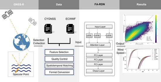
FA-RDN has preferable retrieval capability with relatively high precision and a low dispersion degree of retrieval results at high wind speed. Therefore, it can be used as a new model reference for GNSS-R global sea surface wind speed retrieval.
The remainder of the paper is organized as follows: Section 2 presents the data used in this paper, including original data collection and data pre-processing. Section 3 details the model designed in this paper, including the structure of the model, the model building process, and parameter details. Section 4 introduces the evaluation criteria, comparison models, and experimental design. In Section 5, the experimental results are given and analyzed. Section 6 and Section 7 discuss and summarize the article, respectively, and provide new ideas for future research.

2. Data

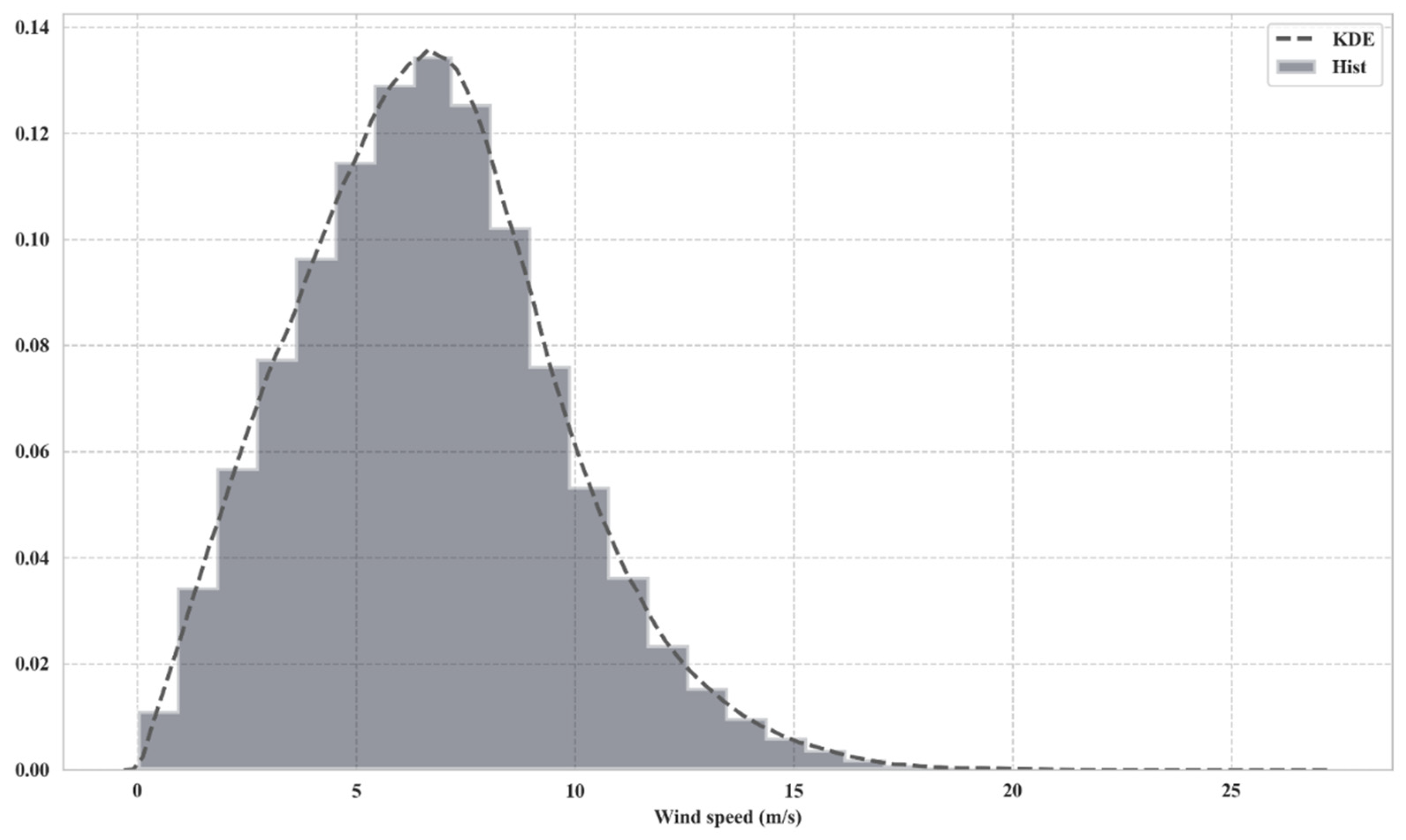
2.1. Data Acquisition

The original data is the L1 band data of the CYGNSS, which consists of eight sub-satellites that can work simultaneously to receive GPS signals reflected from the sea surface with latitude coverage of 38°N to 38°S, and with a spatial resolution of 25 km × 25 km. Figure 1 shows the distribution of specular point trajectories of CYGNSS on 7 August 2019, in which Figure 1A shows the specular point tracks of the CYGNSS 01 satellite, and Figure 1B shows the specular point tracks of 8 CYGNSS satellites. It is evident in Figure 1 that the data type is time series trajectory data, and the data is correlated in the time dimension.
The data spanning from 1 August 2019 to 30 August 2019, are selected as the original data set for training and testing the model. Furthermore, the feature selection refers to the characteristic parameters used in the sea surface wind speed retrieval by the GMF method, the error analysis, and the calibration experience of GNSS-R data. A total of 13 features involving signal attribute, instrument attribute, spatio-temporal attribute and geometry attribute are selected [26,27], as shown in Table 1.
Besides, the European Centre for Medium-Range Weather Forecasts (ECMWF) reanalysis data from the Copernicus Climate Change Service (C3S) climate data repository, which provides global wind speed with a spatio-temporal resolution of 12.5 km × 12.5 km and one hour, are selected as the real sea surface wind speed.

2.2. Data Pre-Processing

To ensure the data quality, the data are quality controlled and screened. The CYGNSS feature data and wind speed with a value of NAN are excluded, the CYGNSS feature data are screened according to the quality control (QC) tags, which are used to filter the data by setting different QC bits, such as spacecraft attitude error, specular point position, data transmission and calibration error, and noise interference or abnormal data, and then the CYGNSS feature data are matched with the ECWMF wind speed data in time and space based on bilinear interpolation. Figure 2 shows the histogram and kernel density estimation of wind speed distribution after spatio-temporal matching. From Figure 2, we can see that the wind speed is mainly in the range of 3~9 m/s, and the number of low and high wind speeds is less compared to the medium wind speed.
Due to the difference in dimension and order of magnitude between feature data, the feature data need to be normalized. The calculation formula is as follows:
h i = h i h m i n h m a x h m i n
By scaling the feature data value to the interval [0, 1], the effects of dimension and order of magnitude are eliminated. It also improves the computational efficiency of the model and accelerates the convergence speed of the model.

3. Method

3.1. Objective

The neural network can be regarded as a complex nonlinear system, which solves regression or classification problems by fitting the nonlinear relationship between input data and the output. GNSS-R sea surface wind speed retrieval is classified as a regression problem. At present, most of the wind speed retrieval network models or GMF models can be expressed as follows:
y t = M ( x t )
M is the designed network model or function model, y t is the wind speed value at time t , x t = [ x t 1 , x t 2 , x t 3 , , x t m ] is the feature data input to the model at that time, and m is the number of feature types.
In this article, we feature of the current moment and plan to mine the historical information of the features. Therefore, the input data of the model are represented by the following matrix:
X t = x t 1 1 x t 1 2 x t 1 m x t 2 1 x t 2 2 x t 2 m x t w 1 x t w 2 x t w m R w × m
w is the time window, that is, the step length of historical information. X t is the input data matrix at this moment, where x i = [ x t 1 i , x t 2 i , x t 3 i , , x t w i ] is the expansion of the i-th feature in the time dimension. The number of feature types is determined by feature engineering, as described in Section 4.3 of the article.
Hence, to satisfy the purpose of mining historical information, we add the LSTM network layer. Besides, to speed up model training efficiency and improve model retrieval accuracy, we add the feature attention mechanism by shifting the weight factor mining from the temporal dimension to the feature type dimension.

3.2. Model and Algorithm
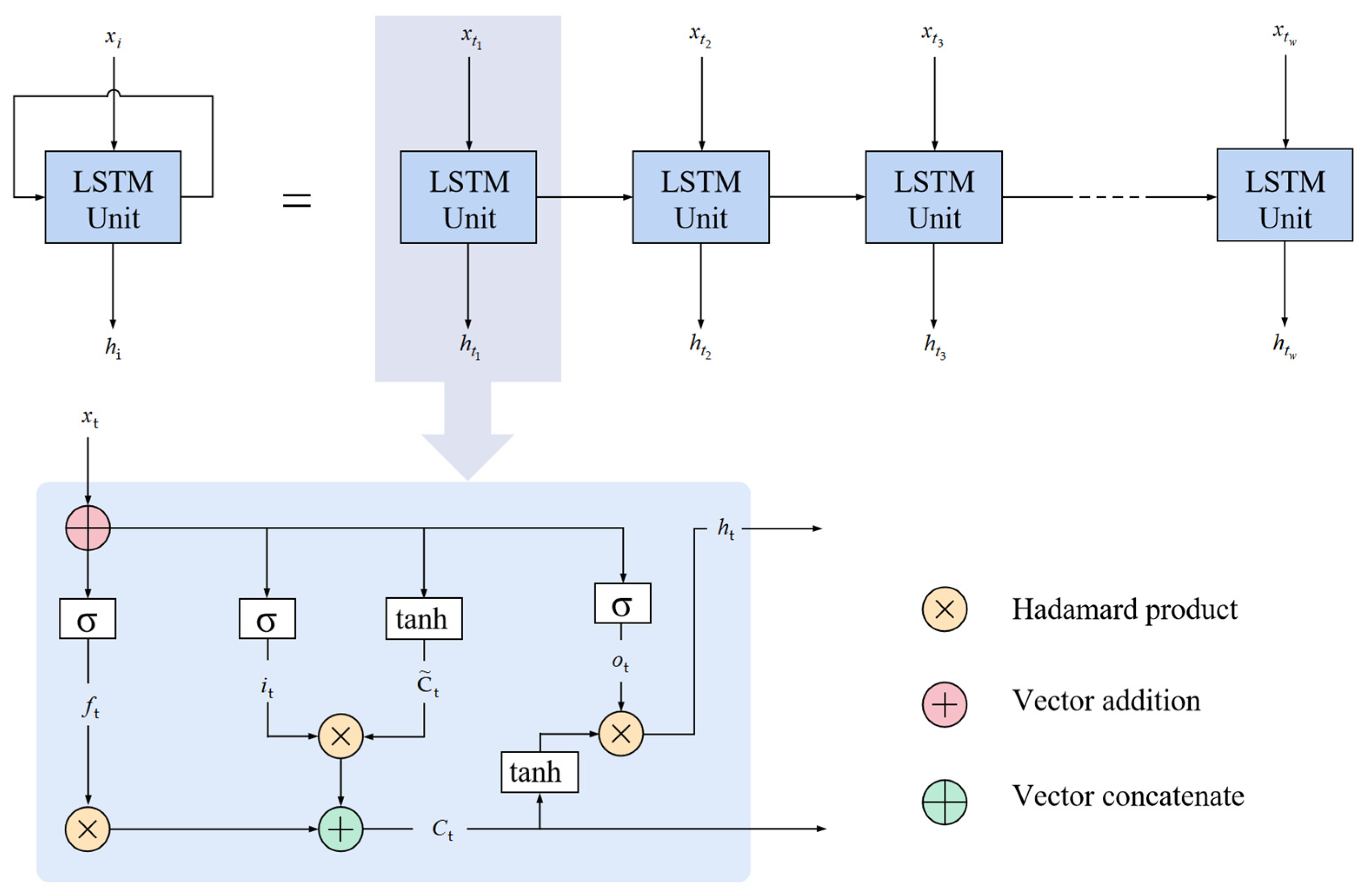
The model consists of five parts: the input layer, the LSTM layer, the feature attention mechanism module, the fully connected layers, and the output layer. The overall structure of the model is shown in Figure 3.
The input layer is utilized to receive the input feature data. LSTM layer realizes time correlation capture of input data. The feature attention mechanism layer calculates the contribution of each feature to the wind speed retrieval and outputs the corresponding weighting factor, which is used for weighting. Then the weighted data is calculated through the fully connected layer, and finally, the wind speed calculated by the model is output through the output layer.

3.2.1. Lstm Layer

The LSTM neural network is a variant of RNN, proposed by Hochreiter and Schmidhuber [28], which solves the problem of vanishing gradient as well as gradient explosion that occurs in RNN [29].
LSTM adjusts the degree of retention, reception, and deletion of node information through gates, including forget gate, input gate, and output gate. The node structure is shown in Figure 4.
The calculation formulas of forget gate, input gate, and output gate are as follows:
f t = σ ( W f [ h t 1 , x t ] + b f )
i t = σ ( W i [ h t 1 , x t ] + b i )
o t = σ ( W o [ h t 1 , x t ] + b o )
Among them, W and b are the weight matrix and bias of the gating mechanism, respectively, h t 1 and x t are the output of the LSTM node at the previous moment and the input feature data at the current moment, respectively. σ is the sigmoid activation function that scales the output to the [0, 1] interval as the control weights. Each gating mechanism realizes the control of the degree of information forgetting, receiving, and output by outputting the control weight of the current node information.
Subsequently, the cell state is updated by short-term memory and gating weight. It is also referred to as long-term memory. The formula for calculating short-term memory C ˜ t is as follows:
C ˜ t = t a n h ( W c [ h t 1 , x t ] + b c )
where W c and b c are the weight matrix and bias term of short-term memory, respectively, and tanh is the tanh activation function. The current cell state is then updated with the following calculation equation.
C t = C t 1 f t + C ˜ t i t
The output of the LSTM layer at the current moment is calculated as follows:
h t = t a n h ( C t ) o t
After that, C t and h t will be passed on to the next moment. LSTM achieves sequence learning by transferring data information in the temporal dimension through cell state and short-term memory.

3.2.2. Attention Mechanism

The attention mechanism is often applied to deal with NLP problems, such as machine translation, public opinion monitoring, and automatic summarization. The idea is derived from the selective attention mechanism of the human brain, which focuses the gaze on key characteristic regions to enhance the efficiency of information utilization [30]. In the NLP problem, we calculate the attention distribution between the current and previous words by the attention mechanism. It can be seen as performing correlation calculations in the time dimension.
The weight is calculated by designing a scoring function score, which calculates the correlation between the current state and the historical state. Typically used scoring functions include the dot product, cosine similarity, and the introduction of an additional neural network layer. In this paper, we use the neural network layer as the scoring function, and the calculation formula is as follows:
S c o r e t = t a n h ( W h i + U h t + b )
where h i is the historical state, W and U are the weights of this network layer, and b is the bias. Then, using the softmax function calculates the scoring result, and the computed result is the weight corresponding to the historical state and the current state. The calculation formula is as follows:
a i = e x p ( S c o r e i ) j = 1 m e x p ( S c o r e j )
However, in the face of regression problems, this weight calculation method is suitable for time-dimensional attention mining that contains only a single feature. In the GNSS-R sea surface wind speed retrieval problem, the input contains multiple characteristic variables. Therefore, we can transfer the attention calculation to the feature type dimension by improving the scoring function. The calculation formula is as follows:
S c o r e i = t a n h ( W v i + U h t w i + b )
where, v i = [ h t 1 i , h t 2 i , , h t w 1 i ] , then the weight factor of the ith feature can be obtained after calculation by softmax function.

3.3. Realization

The implementation of the model includes three phases: data processing, training period of the model, and testing period of the model. The overall process is shown in Figure 5.
The data processing stage provides the dataset used for training and testing the model. The original data collection, data spatio-temporal matching, and quality control are described in Section 2 of the article. Then the time series data are transformed into supervised learning data required for training and testing the network model, D a t a s e t = { ( X 1 , y 1 ) , ( X 2 , y 2 ) , ( X n , y n ) } , and n R is the total amount of data. The data are divided 6:4 into train data set and test data set used in the training and testing phases of the model, respectively. Furthermore, 20% of the data in the training data are reserved as a validation data set, which are utilized to verify and analyze the model after each parameter update to prevent the model from overfitting.
The training process of the neural network is briefly described as updating the weights and biases of each layer of the model to minimize the difference between the output result and the real value. This quantification process is usually implemented by defining a loss function. The loss function selected in proposed model is the same as the one used in previous studies, which is the mean square error (MSE) function [25].
The training process consists of two stages, forward propagation and backward propagation. First, the model parameters, namely the weights and biases of each layer, are initialized randomly [24]. Subsequently, we select a random portion of training data and obtains the wind speed through the forward propagation process. Then a backward propagation process calculates the gradient of the loss function concerning each parameter. The parameters are updated slightly along the gradient direction, and the cycle continues until the optimal model is trained. This model training method is called batch training.
Finally, we evaluate the performance of the trained model by test data. Besides, we compare it with frequently used regression models to validate the designed model’s effectiveness. The specific experiments and their results are shown in Section 4.
In addition, the other hyperparameters of the FA-RDN model are shown in Table 2.

4. Experiment

4.1. Evaluation Criteria

To evaluate the wind speed retrieval results of the FA-RDN model, three evaluation criteria, MSE, root mean square error (RMSE), and mean absolute error (MAE), are used in this paper. The model which obtains the lower results of the above three evaluation criteria means that model’s output is close to the actual wind speed.
MSE = 1 m i = 1 m ( y i y i ) 2
RMSE = 1 m i = 1 m ( y i y i ) 2
MAE = 1 m i = 1 m | ( y i y i ) |
where y is the actual wind speed, y is the wind speed calculated by the model, and m is the total number of test data.
Aiming to represent the enhancement effect of the FA-RDN model more visually, the percentage improvement compared to the comparison model is presented according to MSE, RMSE, and MAE. That is, the percent improvement in MSE ( P MSE ), the percent improvement in RMSE ( P RMSE ), and the percent improvement in MAE ( P MAE ), the comparison models used are described in Section 4.2, and each percent improvement is calculated as follows:
P MSE = MSE 1 MSE 2 MSE 1 × 100 %
P RMSE = RMSE 1 RMSE 2 RMSE 1 × 100 %
P MAE = MAE 1 MAE 2 MAE 1 × 100 %
MSE 1 , RMSE 1 and MAE 1 are calculated from the retrieval results of the comparison model, while MSE 2 , RMSE 2 and MAE 2 are from the FA-RDN model.
In addition, to intuitively reflect the distribution of the retrieval error, we introduce the cumulative distribution function (CDF) of the absolute error (AE) between the model retrieval wind speed and the actual wind speed. The AE calculation formula is as follows:
A E i = | y i y i |
Then the CDF of AE is calculated as follows:
F A E ( x ) = P ( A E x )

4.2. Comparison Model

In this paper, seven comparison models are used to compare and validate the retrieval performance of the FA-RDN model, including four neural network models, Back Propagation Neural Network (BPNN), RNN, LSTM, and ANN, and three machine learning models, RF, eXtreme Gradient Boosting (XGBoost), and Support Vector Regression (SVR).
BPNN, RNN, and LSTM are commonly used neural network models in regression problems. At the same time, LSTM is also used for comparative verification analysis of the effectiveness of attention mechanisms. All models are implemented in Python and built on the Keras platform. The parameters of each neural network model are shown in Table 3.
BPNN: BPNN trains the model using an error backpropagation algorithm based on the gradient descent algorithm and obtains the final model by minimizing the MSE between the model output and the actual value. It is now one of the most used regression models. The BPNN usually consists of an input layer, several hidden layers, and an output layer. In this paper, a BPNN consisting of three hidden layers is built.
RNN: RNN is one of the common regression models, that can model sequence data and obtain the time correlation. The model’s training also uses the backpropagation algorithm.
LSTM: The LSTM is part of the FA-RDN model. See Section 3.1 for a detailed description of the LSTM. The network model architecture and parameters of the LSTM are the same as those of the corresponding components in the FA-RDN, and the LSTM consists of an input layer, LSTM network layer, fully connected layers, and an output layer.
ANN: ANN is a feedforward neural network designed by the literature [22]. Since that paper also studies the GNSS-R-based global sea surface wind speed retrieval problem and selects the feature data from CYGNSS, this model is selected as one of the benchmark models for comparative validation. This model consists of an input layer, two hidden layers, and an output layer with 16 neurons in the hidden layers.
RF: Ensemble learning is a frequently used method in machine learning, which improves classification or regression performance by integrating multiple models [31]. RF is an ensemble learning algorithm based on Decision Tree [32], which has a wide range of applications in classification or regression problems, such as classifying land types based on remote sensing information, estimating SM, and predicting solar radiation [33,34,35].
XGBoost: XGBoost, an ensemble learning method based on tree models, was proposed in 2016 [36]. The basic idea is to combine multiple tree models through continuous iteration to obtain a model with higher accuracy eventually. This method has been used in solving both regression and classification problems [37,38].
SVR: SVR is one of the essential methods in machine learning. It is an applied branch of SVM, specifically used to solve regression problems [39]. The idea of SVR is to search for the optimal hyperplane such that the minimum distance to the hyperplane is obtained for all elements in the original dataset.

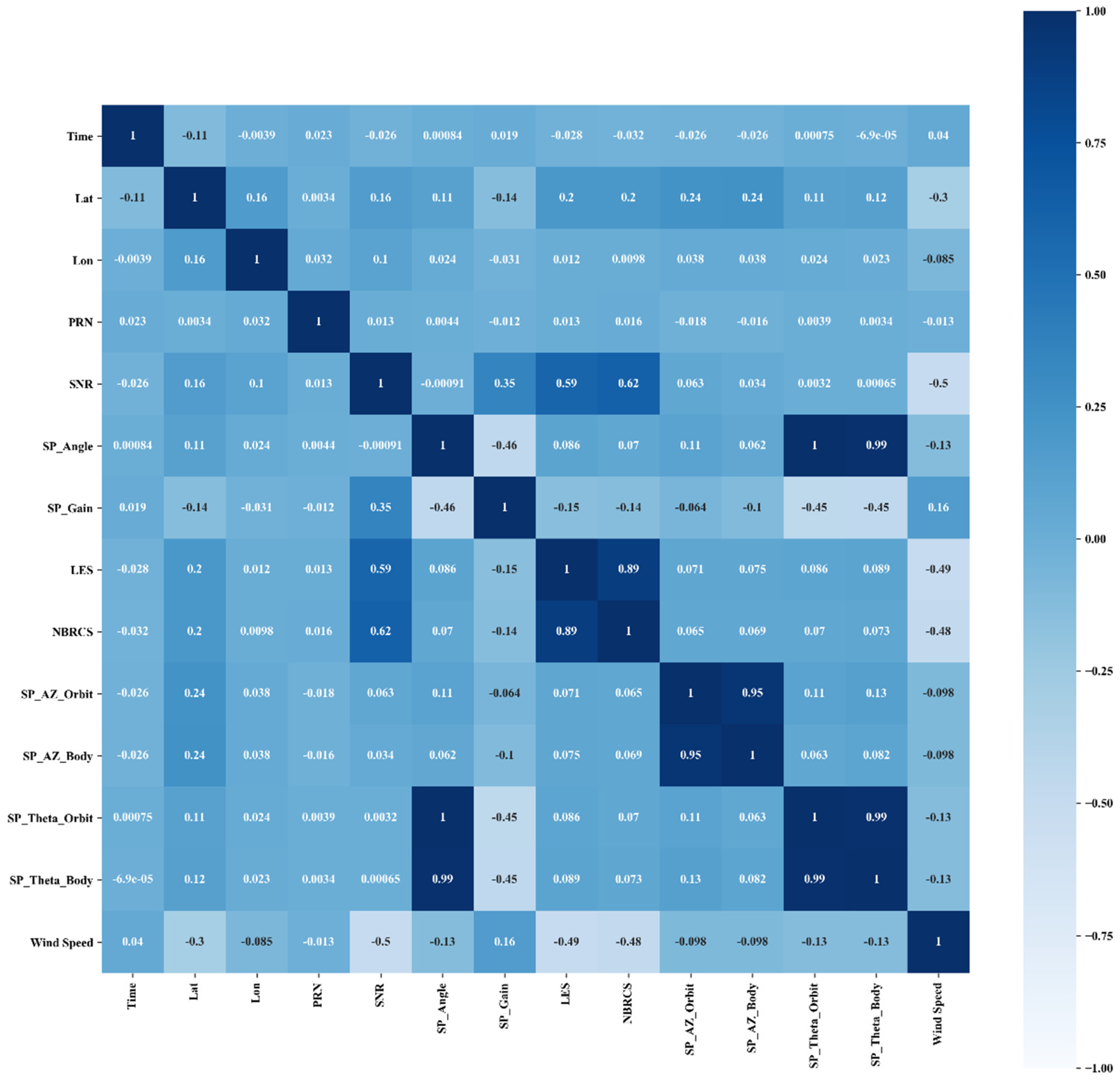
4.3. Feature Engineering

The wide variety of input features is one of the advantages of neural networks compare with GMF methods. The scientific and practical features are critical factors affecting the accuracy of neural network retrieval, so assessing the contribution of different types of features to the retrieval results and selecting the optimal combination of features through feature engineering are essential steps in retrieving sea surface wind speed.
Five data combination schemes are constructed to discuss the effects of spatio-temporal geographic information, spacecraft systems, and attitude information, respectively. All features and corresponding types are listed in Table 1. Each scheme is shown in Table 4. Scheme 1 is the benchmark dataset. The GMF method often selects one or more of SNR, BNRES, and LES as input feature data. For example, NBRCE and LES are chosen in the article [40], and the article [41] usages SNR. Therefore, these three features, SNR, BNRES, and LES, are taken as the benchmark dataset in this article. Scheme 2 discusses the impact of spatiotemporal geographic information: the longitude, latitude, and time of the specular point. Scheme 3 is the effect of the spacecraft system, including antenna gain and PRN. Scheme 4 investigates the influence of spacecraft attitude. We choose the angle between the transmitter to specular point ray and the surface normal and the azimuth angle and theta angle of the specular point to receiver vector in the receiver’s orbit reference frame and body reference frame, respectively.
The retrieval results and analysis of the FA-RDN model under each dataset are presented in Section 5.2.1. Through the feature analysis results, it is possible to analyze the degree of influence of each type of feature on the retrieval result.

4.4. Experimental Design

Comparative experiments and verification experiments are designed to verify the improvement of the FA-RDN model’s retrieval accuracy, evaluate the effectiveness of each module, and analyze the model’s wind speed sensitivity.
A.
Performance evaluation
Firstly, to verify the overall retrieval performance of the FA-RDN model, we compare it with four neural network models, BPNN, RNN, LSTM, and ANN, and three machine learning models, RF, XGBoost, and SVR under each evaluation criteria. Draw the CDF of the AE between the retrieval results and the actual wind speeds to reflect the overall distribution of the retrieval error intuitively.
B.
Validity verification
Secondly, we compare and analyze the retrieval results of the FA-RDN and the LSTM model to verify the effectiveness of the feature attention mechanism. The LSTM’s structure and hyperparameter settings are the same as the FA-RDN model except that the attention mechanism module is not added.
C.
Stability analysis
Intending to realize the practical application of the model in the future, we need to validate the retrieval performance of the model from multiple aspects. The retrieval results of the designed model in the article [23] show high calculated values for low wind speed models and low values for high wind speeds. At the same time, the article [25] also shows that the retrieval error increases gradually with the rise of wind speed at medium and high wind speeds. Therefore, it is necessary to conduct an experimental analysis on the retrieval results of the FA-RDN model at various wind speeds, which is divided according to the Beaufort scale.

5. Experimental Results and Analysis

5.1. Feature Analysis

The retrieval results of the FA-RDN model under each dataset are shown in Table 5, where dataset 1 consisting of SNR, BNRES, LES is the benchmark dataset, dataset 8 contains all features. The percentage improvement of dataset 2, dataset 4, dataset 6 compared to dataset1, and the percentage improvement of dataset 8 compared to dataset 3, dataset 5, dataset 7 under each evaluation criteria are given. Figure 6 is the correlation matrix heatmap which shows the correlation coefficients among features and between each feature and wind speed.
The results presented in Table 5 show that all three types of features improve the retrieval accuracy to a certain extent. The retrieval result of adding the geospatial coordinate information is better than the benchmark dataset, reduces MAE, MSE, and RMSE by 8.56%, 17.38%, and 9.11%, respectively. This result is consistent with the experimental results in the article [22]. The addition of systematic effects and spacecraft attitude information can also improve the retrieval accuracy. The retrieval results of dataset 4 and dataset 6 reduce the MAE, MSE, and RMSE by 5.60% and 6.35%, 10.43% and 12.68%, 5.36% and 6.56%, respectively, compared to the benchmark dataset. Figure 7 describes the trend of retrieval error in each dataset.
As can be seen from Figure 6, among all feature combination schemes, dataset 8 has the best retrieval results. Therefore, this set of features is taken as the final input features for the FA-RDN model.

5.2. Comparative Verification Experiments

5.2.1. Performance Evaluation

A. Comparison results with neural network models
Table 6 lists the retrieval result of the FA-RDN model and the comparison model. It also shows the percentage improvement of the FA-RDN model under each evaluation criteria compared to each comparison model. The bold values in Table 6 represents the optimal value of the evaluation criteria.
It is apparent from Table 6 that the FA-RDN model has the best retrieval result compared with BPNN, RNN, and ANN, reduces MAE by 10.71%, 6.95%, and 13.05%, reduces MSE by 19.67%, 12.73%, and 24.80%, reduces RMSE by 10.38%, 6.58%, and 13.28%, respectively. Moreover, in the evaluation results of the compared models, RNN outperforms BPNN and ANN, which confirms from another perspective that mining historical information helps to improve the inversion accuracy of the models.
Figure 8 shows the scatter plots of model outputs of BPNN, ANN, RNN, and FA-RDN with the ECWMF wind speed, respectively, and the best regression fitting value, the red dashed line x = y. The closer the scatter distribution is to the dotted line, the more accurate the retrieval result of the model is.
In Figure 8, it can be seen that in terms of the overall fit results, the FA-RDN has the best fit, with the overall scatter distribution closest to the red dashed line and the least dispersion, with a Pearson correlation coefficient (Pearson’s r) of 0.879. The second is the RNN model with a Pearson’s r of 0.86, while the third and fourth are BPNN and ANN with Pearson’s r of 0.846 and 0.835, respectively.
B. Comparison results with machine learning models
Table 7 shows the retrieval results for each model and percentage improvement compared to machine learning models. The evaluation criteria results indicate that FA-RDN has the best performance. Compared with RF, XGBoost, and SVR, FA-RDN model reduces MAE by 18.10%, 24.94%, and 27.55%, reduces MSE by 32.57%, 36.42%, and 40.92%, reduces RMSE by 17.89%, 20.26%, and 23.14%, respectively.
Figure 9 presents the AE CDF plots for the FA-RDN model as well as all comparison models. The model with larger function values for a given AE has better performance.
The AE CDF value of the FA-RDN model is always greater than that of the comparison models, which confirms that the FA-RDN model always has a better performance among comparison models.

5.2.2. Validity Verification

To further confirm the effectiveness of the feature attention mechanism in improving the accuracy of wind speed retrieval, the FA-RDN model is compared with the LSTM model in that experiment. The experimental results are shown in Table 8.
The retrieval result of the FA-RDN model is better than the comparison model, and reduces the MAE, MSE, and RMSE by 5.78%, 10.45%, and 5.37%, respectively. It further confirms the effectiveness of the attention mechanism in improving the wind speed retrieval accuracy.

5.2.3. Stability Analysis

Figure 10 shows the retrieval results and the amount of data at different wind speeds, which are divided refer to the Beaufort scale. This figure can also be seen as a numerical representation of Figure 8D.
As can be seen in Figure 10, FA-RDN has higher retrieval accuracy in light air to strong breeze, that is, wind speeds from 0.3 m/s to 13.9 m/s. In calm and moderategale, that is, wind speed from 0.0 m/s to 0.3 m/s and from 13.9 m/s to 17.2 m/s, the retrieval error increases slightly, and has a significant increase after the wind speed is higher than 20.8 m/s. This result is consistent with the result of article [25], that is, in calm and higher wind speed, the retrieval results are worse than low and medium wind speed. In general, the FA-RDN model has less error fluctuation and better stability under the wind speed range of 20.8 m/s.

6. Discussion

In the feature analysis, all datasets are divided into five groups based on different combinations of features, as shown in Table 5. The percentage improvement after adding different types of features compared to the baseline dataset is compared separately by experiment. The experiments confirm that adding the selected feature types, i.e., spatio-temporal geographic information, spacecraft systems, and attitude information, all influence the overall retrieval results. After comparing the retrieval results of all datasets under each evaluation metric, as shown in Figure 6, the final input feature scheme is selected for the designed model, that is, dataset8 with all features is added, which improves MAE, MSE, and RMSE by 20.22%, 37.15%, and 20.72%, respectively, compared with the benchmark dataset. However, it is worth noting that the three feature types mentioned above are still the result of manual selection after analysis. In the follow-up research, we are designing an end-to-end retrieval model that can expand the selection range of feature types, and has the ability to automatically select feature types that have a proportional boost to the retrieval results [42].
Table 6, Table 7 and Table 8 list the retrieval results of each model, and Figure 7 shows the fitting between the retrieval results of the model and the true value of wind speed. The FA-RDN model has optimal results for each evaluation metric, MAE, MSE, and RMSE, with results of 1.08 m/s, 2.10 m/s, and 1.45 m/s, respectively. Besides, the overall density distribution and the distribution of the highest density for the fitted scatter of the designed model are closest to the x = y line, having the smallest offset at high wind speeds and the highest Pearson’s r value of 0.879 compared to other network models. Meanwhile, RNN has suboptimal retrieval result, which further confirms that mining the data’s temporal correlation information helps improve retrieval accuracy. In combination with Figure 9, the retrieval results are inferior at high wind speeds compared to low and medium wind speeds. This result may be due to the low sensitivity of the CYGNSS L1 observations at high wind speeds [40,43], and the small percentage of data samples at high wind speeds, see Figure 2. Therefore, in the future study, in addition to further expanding the selection of model input features, it is planned to add sea surface information to assist in the retrieval, such as sea surface height, wavelength, wave direction, and alleviate the data imbalance problem to improve the model retrieval accuracy.

7. Conclusions

This paper proposes a hybrid network model for the retrieval of global sea surface wind speeds. The recurrent deep neural network using improved attention mechanism can mine the temporal correlation information of the input features from the temporal dimension. The original data is from the L1 band data of the CYGNSS and the ECMWF. We compare and analyze the influence of temporal-spatial geographical features, systematic effects, and spacecraft attitude information on the retrieval accuracy through feature engineering.
It is confirmed that the FA-RDN model has better wind speed retrieval results, reducing the RMSE by 12% to 40% compared to all comparison models. Moreover, the retrieval results verify the effectiveness of the attention mechanism in optimizing the retrieval results and the historical reference information that helps to improve the model’s accuracy. In general, this paper provides a feature reference and a new reference model for retrieving GNSS-R sea surface wind speed based on neural network.
In future research, in addition to the temporal dimension, information can also be added for reference from a spatial perspective. Satellites network observations can be carried out to simultaneously extract information on the spatial correlation between multiple reflection points. Besides, further research and experiments can be conducted on the architecture of the network model.

Author Contributions

Conceptualization, X.L. and W.B.; methodology, X.L.; software, X.L., C.Y.; validation, X.L., W.B., J.X., P.H.; formal analysis, X.L., F.H.; investigation, X.L.; resources, Q.D., X.M.; data curation, X.L., J.X.; writing—original draft preparation, X.L.; writing—review and editing, W.B., F.H., G.T.; visualization, X.L., G.T.; supervision, W.B.; project administration, Y.S.; funding acquisition, C.L., Q.D. All authors have read and agreed to the published version of the manuscript.

Funding

This research was funded by the National Natural Science Foundation of China, grant numbers 42074042 and 41775034.

Acknowledgments

We acknowledge the reviewers for their careful review and constructive suggestions, which have helped improve this article, NASA for the CYGNSSS public data, ECMWF for the reanalysis data, and the support of the funding of national space science center, Chinese academy.

Conflicts of Interest

The authors declare no conflict of interest.

Abbreviations

AEAbsolute error
ANNArtificial Neural Network
BPNNBackpropagation neural network
CDFCumulative distribution function
CYGNSSCyclone Global Navigation Satellite System
DDMDelay-Doppler map
GMFGeophysical model function
FA-RDNRecurrent deep neural network using feature attention mechanism
LESLeading edge of the slope
LSTMLong-short term memory
MAEMean absolute error
MLPMultilayer Perceptron
MSEMean square error
NBRCSNormalized bistatic radar cross-section
NLPNatural Language Processing
Pearson’s rPearson correlation coefficient
P M A E Percent improvement in MAE
P M S E Percent improvement in MSE
P R M S E Percent improvement in RMSE
PRNGPS pseudo random noise code
RMSERoot mean square error
RNNRecurrent Neural Network
RFRandom Forest
SMSoil moisture
SNRDDM signal to noise ratio
SP_AngleThe angle between the transmitter to specular point ray and the surface normal
SP_AZ_bodyThe azimuth angle of the specular point to receiver vector in the receiver’s body reference frame
SP_AZ_orbitThe azimuth angle of the specular point to receiver vector in the receiver’s orbit reference frame
SP_gainThe antenna gain towards specular point
SP_LatThe latitude of the specular point
SP_LonThe longitude of the specular point
SP_Theta_bodyThe theta angle of the specular point to receiver vector in the receiver’s body reference frame
SP_Theta_orbitThe theta angle of the specular point to receiver vector in the receiver’s orbit reference frame
SP_TimeThe time of the specular point
SVMSupport Vector Machine
SVRSupport Vector Regression
TDS-1Demonstration Satellite-1
UK-DMCUnited Kingdom-Disaster Monitoring Constellation Technology
XGBoosteXtreme Gradient Boosting

References

  1. Martín-Neira, M. A passive reflectometry and interferometry system (PARIS) application to ocean altimetry. ESA J. 1993, 17, 331–355. [Google Scholar]
  2. Auber, J.; Bibaut, A.; Rigal, J. Characterization of Multipath on Land and Sea at GPS Frequencies. In Proceedings of the 7th International Technical Meeting of the Satellite Division of the Institute of Navigation (ION GPS 1994), Salt Lake City, UT, USA, 20–23 September 1994; pp. 1155–1171. [Google Scholar]
  3. Garrison, J.; Katzberg, S.; Hill, M. Effect of sea roughness on bistatically scattered range coded signals from the Global Positioning System. Geophys. Res. Lett. 1998, 25, 2257–2260. [Google Scholar] [CrossRef] [Green Version]
  4. Clarizia, M.P.; Gommenginger, C.; Bisceglie, M.; Galdi, C.; Srokosz, M. Simulation of L-Band Bistatic Returns from the Ocean Surface: A Facet Approach with Application to Ocean GNSS Reflectometry. IEEE Trans. Geosci. Remote Sens. 2012, 50, 960–971. [Google Scholar] [CrossRef]
  5. Gleason, S.; Hodgart, S.; Sun, Y.P.; Gommenginger, C.; Mackin, S.; Adjrad, M.; Unwin, M. Detection and Processing of bistatically reflected GPS signals from low Earth orbit for the purpose of ocean remote sensing. IEEE Trans. Geosci. Remote Sens. 2005, 43, 1229–1241. [Google Scholar] [CrossRef] [Green Version]
  6. Foti, G.; Gommenginger, C.; Jales, P.; Unwin, M.; Shaw, A.; Robertson, C.; Roselló, J. Spaceborne GNSS Reflectometry for Ocean Winds: First Results from the UK TechDemoSat-1 Mission. Geophys. Res. Lett. 2015, 42, 5435–5441. [Google Scholar] [CrossRef] [Green Version]
  7. Foti, G.; Gommenginger, C.; Unwin, M.; Jales, P.; Tye, J.; Roselló, J. An Assessment of Non-Geophysical Effects in Spaceborne GNSS Reflectometry Data from the UK TechDemoSat-1 Mission. IEEE J. Sel. Top. Appl. Earth Obs. Remote Sens. 2017, 10, 3418–3429. [Google Scholar] [CrossRef] [Green Version]
  8. Soisuvarn, S.; Jelenak, Z.; Said, F.; Chang, P.; Egido, A. The GNSS Reflectometry Response to the Ocean Surface Winds and Waves. IEEE J. Sel. Top. Appl. Earth Obs. Remote Sens. 2016, 9, 4678–4699. [Google Scholar] [CrossRef]
  9. Clarizia, M.P.; Ruf, C. Wind Speed Retrieval Algorithm for the Cyclone Global Navigation Satellite System (CYGNSS) Mission. IEEE Trans. Geosci. Remote Sens. 2016, 54, 4419–4432. [Google Scholar] [CrossRef]
  10. Unwin, M.; Jales, P.; Blunt, P.; Duncan, S.; Brummitt, M.; Ruf, C. The SGR-ReSI and its application for GNSS reflectometry on the NASA EV-2 CYGNSS mission. In Proceedings of the 2013 IEEE Aerospace Conference, Big Sky, MT, USA, 2–9 March 2013; pp. 1–6. [Google Scholar]
  11. Komjathy, A.; Armatys, M.; Masters, D.; Axelrad, P.; Zavorotny, V.; Katzberg, S. Retrieval of Ocean Surface Wind Speed and Wind Direction Using Reflected GPS Signals. J. Atmos. Ocean Technol. 2004, 21, 515–526. [Google Scholar] [CrossRef] [Green Version]
  12. Cardellach, E.; Fabra, F.; Nogués-Correig, O.; Oliveras, S.; Ribó, S.; Rius, A. GNSS-R ground-based and airborne campaigns for ocean, land, ice, and snow techniques: Application to the GOLD-RTR data sets. Radio Sci. 2011, 46, 1–16. [Google Scholar] [CrossRef] [Green Version]
  13. Yan, Q.; Huang, W.; Jin, S.; Jia, Y. Pan-tropical soil moisture mapping based on a three-layer model from CYGNSS GNSS-R data. Remote Sens. Environ. 2020, 247, 111944. [Google Scholar] [CrossRef]
  14. Stilla, D.; Zribi, M.; Pierdicca, N.; Baghdadi, N.; Huc, M. Desert Roughness Retrieval Using CYGNSS GNSS-R Data. Remote Sens. 2020, 12, 743. [Google Scholar] [CrossRef] [Green Version]
  15. Carreno-Luengo, H.; Luzi, G.; Crosetto, M. Above-Ground Biomass Retrieval over Tropical Forests: A Novel GNSS-R Approach with CyGNSS. Remote Sens. 2020, 12, 1368. [Google Scholar] [CrossRef]
  16. Jacobson, M.; Emery, W.; Westwater, E. Oceanic wind vector determination using a dual-frequency microwave airborne radiometer theory and experiment. In Proceedings of the 1996 International Geoscience and Remote Sensing Symposium (IGARSS ’96.), Lincoln, NE, USA, 31 May 1996; Volume 2, pp. 1138–1140. [Google Scholar]
  17. Monaldo, F.; Thompson, D.R.; Beal, R.; Pichel, W.; Clemente-Colon, P. Comparison of SAR-derived wind speed with model predictions and ocean buoy measurements. IEEE Trans. Geosci. Remote Sens. 2001, 39, 2587–2600. [Google Scholar] [CrossRef]
  18. Clarizia, M.P.; Ruf, C.; Jales, P.; Gommenginger, C. Spaceborne GNSS-R Minimum Variance Wind Speed Estimator. IEEE Trans. Geosci. Remote Sens. 2014, 52, 6829–6843. [Google Scholar] [CrossRef]
  19. Frate, F.; Pacifici, F.; Schiavon, G.; Solimini, C. Use of Neural Networks for Automatic Classification from High-Resolution Images. IEEE Trans. Geosci. Remote Sens. 2007, 45, 800–809. [Google Scholar] [CrossRef]
  20. Chi, M.; Feng, R.; Bruzzone, L. Classification of hyperspectral remote-sensing data with primal SVM for small-sized training dataset problem. Adv. Space Res. 2008, 41, 1793–1799. [Google Scholar] [CrossRef]
  21. Eroglu, O.; Kurum, M.; Boyd, D.; Gürbüz, A.C. High Spatio-Temporal Resolution CYGNSS Soil Moisture Estimates Using Artificial Neural Networks. Remote Sens. 2019, 11, 2272. [Google Scholar] [CrossRef] [Green Version]
  22. Reynolds, J.; Clarizia, M.P.; Santi, E. Wind Speed Estimation from CYGNSS Using Artificial Neural Networks. IEEE J. Sel. Top. Appl. Earth Obs. Remote Sens. 2020, 13, 708–716. [Google Scholar] [CrossRef]
  23. Asgarimehr, M.; Zhelavskaya, I.; Foti, G.; Reich, S.; Wickert, J. A GNSS-R Geophysical Model Function: Machine Learning for Wind Speed Retrievals. IEEE Geosci. Remote Sens. Lett. 2020, 17, 1333–1337. [Google Scholar] [CrossRef]
  24. Liu, Y.; Collett, I.; Morton, Y. Application of Neural Network to GNSS-R Wind Speed Retrieval. IEEE Trans. Geosci. Remote Sens. 2019, 57, 9756–9766. [Google Scholar] [CrossRef]
  25. Chu, X.; He, J.; Song, H.; Qi, Y.; Sun, Y.; Bai, W.; Li, W.; Wu, Q. Multimodal Deep Learning for Heterogeneous GNSS-R Data Fusion and Ocean Wind Speed Retrieval. IEEE J. Sel. Top. Appl. Earth Obs. Remote Sens. 2020, 13, 5971–5981. [Google Scholar] [CrossRef]
  26. Balasubramaniam, R.; Ruf, C. Neural Network Based Quality Control of CYGNSS Wind Retrieval. Remote Sens. 2020, 12, 2859. [Google Scholar] [CrossRef]
  27. Gleason, S.; Ruf, C.S.; O’Brien, A.J.; McKague, D.S. The CYGNSS Level 1 Calibration Algorithm and Error Analysis Based on On-Orbit Measurements. IEEE J. Sel. Top. Appl. Earth Obs. Remote Sens. 2019, 12, 37–49. [Google Scholar] [CrossRef]
  28. Hochreiter, S.; Schmidhuber, J. Long Short-Term Memory. Neural Comput. 1997, 9, 1735–1780. [Google Scholar] [CrossRef] [PubMed]
  29. Bengio, Y.; Simard, P.; Frasconi, P. Learning long-term dependencies with gradient descent is difficult. IEEE Trans. Neural Netw. 1994, 5, 157–166. [Google Scholar] [CrossRef] [PubMed]
  30. Kastner, S.; Ungerleider, L.G. Mechanisms of Visual Attention in the Human Cortex. Annu. Rev. Neurosci. 2000, 23, 315–341. [Google Scholar]
  31. Zhou, Z.-H. Ensemble Methods: Foundations and Algorithms; Chapman and Hall/CRC: London, UK, 2012; Volume 14, ISBN 978-1-4398-3003-1. [Google Scholar]
  32. Rodriguez-Galiano, V.F.; Ghimire, B.; Rogan, J.; Chica-Olmo, M.; Rigol-Sanchez, J.P. An Assessment of the Effectiveness of a Random Forest Classifier for Land-Cover Classification. ISPRS J. Photogramm. Remote Sens. 2012, 67, 93–104. [Google Scholar] [CrossRef]
  33. Senyurek, V.; Lei, F.; Boyd, D.; Kurum, M.; Gurbuz, A.C.; Moorhead, R. Machine Learning-Based CYGNSS Soil Moisture Estimates over ISMN Sites in CONUS. Remote Sens. 2020, 12, 1168. [Google Scholar] [CrossRef] [Green Version]
  34. Cutler, A.; Cutler, D.; Stevens, J. Random Forests. In Machine Learning—ML; Springer: Boston, MA, USA, 2011; Volume 45, pp. 157–176. ISBN 978-1-4419-9325-0. [Google Scholar]
  35. Benali, L.; Notton, G.; Fouilloy, A.; Voyant, C.; Dizene, R. Solar Radiation Forecasting Using Artificial Neural Network and Random Forest Methods: Application to Normal Beam, Horizontal Diffuse and Global Components. Renew. Energy 2019, 132, 871–884. [Google Scholar] [CrossRef]
  36. Chen, T.; Guestrin, C. XGBoost: A Scalable Tree Boosting System. In Proceedings of the 22nd ACM SIGKDD International Conference on Knowledge Discovery and Data Mining, New York, NY, USA, 13–17 August 2016; pp. 785–794. [Google Scholar] [CrossRef] [Green Version]
  37. Bhattacharya, S.; Maddikunta, P.K.R.; Kaluri, R.; Singh, S.; Gadekallu, T.R.; Alazab, M.; Tariq, U. A Novel PCA-Firefly Based XGBoost Classification Model for Intrusion Detection in Networks Using GPU. Electronics 2020, 9, 219. [Google Scholar] [CrossRef] [Green Version]
  38. Zamani Joharestani, M.; Cao, C.; Ni, X.; Bashir, B.; Talebiesfandarani, S. PM2.5 Prediction Based on Random Forest, XGBoost, and Deep Learning Using Multisource Remote Sensing Data. Atmosphere 2019, 10, 373. [Google Scholar] [CrossRef] [Green Version]
  39. Drucker, H.; Burges, C.J.C.; Kaufman, L.; Smola, A.; Vapnik, V. Support Vector Regression Machines. In Proceedings of the 9th International Conference on Neural Information Processing Systems, Denver, CO, USA, 3 December 1996; MIT Press: Cambridge, MA, USA, 1996; pp. 155–161. [Google Scholar]
  40. Ruf, C.S.; Balasubramaniam, R. Development of the CYGNSS Geophysical Model Function for Wind Speed. IEEE J. Sel. Top. Appl. Earth Obs. Remote Sens. 2019, 12, 66–77. [Google Scholar] [CrossRef]
  41. Asgarimehr, M.; Wickert, J.; Reich, S. TDS-1 GNSS Reflectometry: Development and Validation of Forward Scattering Winds. IEEE J. Sel. Top. Appl. Earth Obs. Remote Sens. 2018, 11, 4534–4541. [Google Scholar] [CrossRef]
  42. Ferreira, A.J.; Figueiredo, M.A.T. Efficient Feature Selection Filters for High-Dimensional Data. Pattern Recognit. Lett. 2012, 33, 1794–1804. [Google Scholar] [CrossRef] [Green Version]
  43. Ruf, C.S.; Gleason, S.; McKague, D.S. Assessment of CYGNSS Wind Speed Retrieval Uncertainty. IEEE J. Sel. Top. Appl. Earth Obs. Remote Sens. 2019, 12, 87–97. [Google Scholar] [CrossRef]
Figure 1. Distribution of specular point trajectories of CYGNSS on 7 August 2019. (A)Specular point tracks of the CYGNSS 01 satellite. (B) Specular point tracks of 8 CYGNSS satellites.
Remotesensing 13 04820 g001
Figure 2. Wind speed quantity distribution.
Remotesensing 13 04820 g002
Figure 3. Structure of the FA-RDN model.
Remotesensing 13 04820 g003
Figure 4. LSTM network layer structure and node structure.
Remotesensing 13 04820 g004
Figure 5. The FA-RDN model implementation process.
Remotesensing 13 04820 g005
Figure 6. The correlation matrix heatmap which shows the correlation coefficients among features and between each feature and wind speed.
Remotesensing 13 04820 g006
Figure 7. The trend of retrieval error in each dataset.
Remotesensing 13 04820 g007
Figure 8. Comparison of model retrieval output with the true value of wind speed. (A) BPNN retrieval results. (B) ANN retrieval results. (C) RNN retrieval results. (D) FA-RDN retrieval results.
Remotesensing 13 04820 g008
Figure 9. CDF comparison of the FA-RDN model with all comparison models.
Remotesensing 13 04820 g009
Figure 10. The amount of data and the retrieval results of the FA-RDN model at different wind speed.
Remotesensing 13 04820 g010
Table 1. List of selected features.
NONameType
1SNRSignal attribute
2NBRCSSignal attribute
3LESSignal attribute
4SP_gainInstrument attribute
5PRNInstrument attribute
6SP_Lon Spatio-temporal attribute
7SP_LatSpatio-temporal attribute
8SP_TimeSpatio-temporal attribute
9SP_AngleGeometry attribute
10SP_AZ_orbitGeometry attribute
11SP_AZ_bodyGeometry attribute
12SP_Theta_orbitGeometry attribute
13SP_Theta_bodyGeometry attribute
Table 2. Hyperparameters configuration of FA-RDN model.
HyperparameterSize/TypeDefinition/Application
Batch size64The size of the dataset that uses part of the training data to complete the training once and update the network weights.
Activation function f ( x ) = x 1 + | x | It is used for model computation, providing nonlinearity to the model, and improving the expressiveness of the network.
Loss functionMSEThe way of measuring the difference between the computed output of the network and the true value in the training process.
OptimizerAdamThe way to calculate the optimal weights as well as bias of neural network through loss function.
EpochIn this article, it is determined by early termination.The number of a complete traversal of the entire train dataset at training time.
Table 3. Comparison model’s parameters.
ModelParameterValue
BPNNHidden neurons
Number of hidden layers
{32,16,16}
{3}
RNNHidden neurons
Number of RNN layers
Number of FC layers
{13,16,16,8}
{1}
{3}
LSTMHidden neurons
Number of LSTM layers
Number of FC layers
{13,16,16,8}
{1}
{3}
ANNHidden neurons
Number of hidden layers
{16,16}
{2}
Table 4. The scheme of feature division.
SchemeDatasetFeatures
1Dataset 1SNR, BNRES, and LES (benchmark dataset)
2Dataset 2Benchmark dataset + spatio-temporal attribute
Dataset 3All features − spatio-temporal attribute
3Dataset 4Benchmark dataset + instrument attribute
Dataset 5All features − instrument attribute
4Dataset 6Benchmark dataset + geometry attribute
Dataset 7All features − geometry attribute
5Dataset 8All features
Table 5. Characteristic analysis.
MetricsImprovement
MAEMSERMSEPMAEPMSEPRMSE
Dataset 11.363.341.83\\\
Dataset 21.242.761.668.56%17.38%9.11%
Dataset 41.282.991.735.60%10.43%5.36%
Dataset 61.272.911.716.35%12.68%6.56%
Dataset 31.252.821.6813.55%25.65%13.77%
Dataset 51.212.621.6210.64%20.12%10.63%
Dataset 71.212.581.6110.30%18.73%9.85%
Dataset 81.082.101.45\\\
Table 6. Experimental results of comparison and verification of retrieval performance.
MetricsImprovement
MAEMSERMSEPMAEPMSEPRMSE
BPNN1.212.611.6210.71%19.67%10.38%
RNN1.172.401.556.95%12.73%6.58%
ANN1.252.791.6713.05%24.80%13.28%
FA_RDN1.082.101.45\\\
Table 7. Retrieval results for each model and percentage improvement compared to machine learning models.
MetricsImprovement
MAEMSERMSEPMAEPMSEPRMSE
RF1.323.111.7618.10%32.57%17.89%
XGBoost1.453.301.8224.94%36.42%20.26%
SVR1.503.551.8827.55%40.92%23.14%
FA-RDN1.082.101.45\\\
Table 8. Experimental results of verification of the effectiveness of the attention mechanism.
MetricsImprovement
MAEMSERMSEPMAEPMSEPRMSE
LSTM1.152.341.535.78%10.45%5.37%
FA_RDN1.082.101.45\\\
Publisher’s Note: MDPI stays neutral with regard to jurisdictional claims in published maps and institutional affiliations.

