Article

Experimental Assessment of UWB and Vision-Based Car Cooperative Positioning System

1
Department of Civil and Environmental Engineering, University of Florence, 50139 Florence, Italy
2
Department of Civil, Environmental and Geodetic Engineering, The Ohio State University, Columbus, OH 43210, USA
3
Department of Geodesy and Geoinformation, TU Wien-Vienna University of Technology, 1040 Vienna, Austria
4
Department of Geospatial Science, RMIT University, Melbourne, VIC 3000, Australia
5
School of Rural and Surveying Engineering, National Technical University of Athens, 157 73 Athens, Greece
6
College of Engineering, The Ohio State University, Columbus, OH 43210, USA
*
Author to whom correspondence should be addressed.
Remote Sens. 2021, 13(23), 4858; https://0-doi-org.brum.beds.ac.uk/10.3390/rs13234858
Submission received: 10 September 2021 / Revised: 8 November 2021 / Accepted: 24 November 2021 / Published: 30 November 2021

Abstract

:
The availability of global navigation satellite systems (GNSS) on consumer devices has caused a dramatic change in every-day life and human behaviour globally. Although GNSS generally performs well outdoors, unavailability, intentional and unintentional threats, and reliability issues still remain. This has motivated the deployment of other complementary sensors in such a way that enables reliable positioning, even in GNSS-challenged environments. Besides sensor integration on a single platform to remedy the lack of GNSS, data sharing between platforms, such as in collaborative positioning, offers further performance improvements for positioning. An essential element of this approach is the availability of internode measurements, which brings in the strength of a geometric network. There are many sensors that can support ranging between platforms, such as LiDAR, camera, radar, and many RF technologies, including UWB, LoRA, 5G, etc. In this paper, to demonstrate the potential of the collaborative positioning technique, we use ultra-wide band (UWB) transceivers and vision data to compensate for the unavailability of GNSS in a terrestrial vehicle urban scenario. In particular, a cooperative positioning approach exploiting both vehicle-to-infrastructure (V2I) and vehicle-to-vehicle (V2V) UWB measurements have been developed and tested in an experiment involving four cars. The results show that UWB ranging can be effectively used to determine distances between vehicles (at sub-meter level), and their relative positions, especially when vision data or a sufficient number of V2V ranges are available. The presence of NLOS observations is one of the principal factors causing a decrease in the UWB ranging performance, but modern machine learning tools have shown to be effective in partially eliminating NLOS observations. According to the obtained results, UWB V2I can achieve sub-meter level of accuracy in 2D positioning when GNSS is not available. Combining UWB V2I and GNSS as well V2V ranging may lead to similar results in cooperative positioning. Absolute cooperative positioning of a group of vehicles requires stable V2V ranging and that a certain number of vehicles in the group are provided with V2I ranging data. Results show that meter-level accuracy is achieved when at least two vehicles in the network have V2I data or reliable GNSS measurements, and usually when vehicles lack V2I data but receive V2V ranging to 2–3 vehicles. These working conditions typically ensure the robustness of the solution against undefined rotations. The integration of UWB with vision led to relative positioning results at sub-meter level of accuracy, an improvement of the absolute positioning cooperative results, and a reduction in the number of vehicles required to be provided with V2I or GNSS data to one.

Graphical Abstract

1. Introduction

Localisation in partially obscured GNSS (global navigation satellite systems) environments and indoors is challenging, as a GNSS receiver on its own cannot provide a precise, robust, and high-level positioning solution in these environments. Consequently, sensor integration and fusion based on new approaches are required. Previous work of the authors has focused on the use of ultra-wide band (UWB) [1], wireless fidelity (Wi-Fi) [2], vision-based positioning with cameras and light detection and ranging (LiDAR) [3], as well as inertial sensors in different scenarios in GNSS-denied and challenged combined outdoor/indoor and transitional environments. Retscher et al. [1] provide a comprehensive summary of the test scenarios and experimental sensor setups used in an one-week data collection campaign carried out at The Ohio State University (OSU), under the joint IAG (International Association of Geodesy) and FIG (Federation of Surveyors) working group (WG) on multi-sensor systems. Several scenarios are described for localisation and navigation of mobile sensor platforms, including vehicles, bicyclists, and pedestrians. The major aim of the WG is to achieve a cooperative, robust, and ubiquitous positioning solution of mobile platforms for intelligent transport systems (ITS). For that purpose, a cooperative positioning (CP) solution based on the GNSS, UWB, and vision-based data is investigated in this paper.Since GNSS is the most used positioning technology worldwide, its use, when available, is obvious. UWB and vision are expected to synergistically contribute to handling GNSS unavailability. To be more specific, UWB can be used as a stand-alone positioning solution in small areas when the required accuracy is at sub-meter level. Unfortunately, its stand-alone usability on large areas requires the use of a large infrastructure, because the UWB measurement success rate quickly decreases with the distance between the devices. However, vision can be used even at quite large distances, as it provides a different kind of information (i.e., angles instead of ranges); hence, its combination with UWB shall reduce the size of the required UWB infrastructure and/or improve the overall positioning results.
CP refers to an integrated positioning solution employing multiple location sensors with different accuracy on different platforms for sharing of their absolute and relative localisation. CP solutions have been demonstrated to be useful for positioning and navigation of mobile platforms operating in swarms or networks. However, these solutions are mainly based on integration of inertial sensors with GNSS and/or radio signals [4,5,6]. The work of the joint IAG/FIG WG focuses on the use of alternative positioning, navigation and timing (PNT) techniques in combination with commonly employed localisation techniques and sensors. As a part of the OSU field campaign, a set of outdoor data was collected with a major aim of providing benchmark data for further research on navigation and integrity monitoring solutions. Especially, the application for ubiquitous CP localisation and navigation for intelligent transport systems (ITS) in urban environments is a major focus of the work of the WG.
Collaborative/cooperative navigation represents the next level in generalization of the sensor integration concept, which is classically referred to integrating all the sensory data streams acquired on a single platform. CP provides a framework to integrate sensor data acquired by multiple platforms that generally operate in close proximity to each other, such as a group of vehicles on a road section or a swarm of UAS. The two requirements for effective CP are the availability of internode communication and ranging. Recent technological developments, in particular, autonomous vehicle technologies, already provide the necessary sensor and communication capabilities for experimental CP implementations. For our investigation, we use UWB-based ranging and explore the potential of combining it with optical imagery. These sensors are easily available and tested in other applications, and thus they form a good basis for demonstration, allowing us to focus on the CP computation and performance aspects. Obviously, any other ranging sensor can be used instead of UWB. There are several approaches to obtain an optimal navigation solution for a group of platforms, depending on what data is shared among the platforms, such as all sensory data or just locally computed navigation solutions, etc. The data sharing is primarily a communication task, mainly optimizing the amount of data transferred in the network for a given bandwidth. Note that this communication part is not addressed here, which is a challenging topic on its own. In terms of computations, the central solution may produce the theoretically optimal results, as it integrates all the sensory data in the navigation filter. Then, there are local navigation solutions computed and shared and several other solutions in between. In this study, our focus is on the exploitation of the network geometry created by the platforms, which is used as constrains in the navigation solution. For simplicity, we use the widely known terms of vehicle-to-infrastructure (V2I) and vehicle-to-vehicle (V2V) to differentiate between the various range measurements.
To demonstrate the performance of the proposed CP methods, an ad hoc vehicle network with infrastructure nodes equipped with UWB radios was set up. Two scenarios were considered in the experiments. The first part aimed to collect the data when vehicles are driving in different formations along the road, and the second part was focused on intersection area positioning where the cars are performing different manoeuvres. As a result, collected data provide opportunity for further research on optimal CP network geometries given a specific ITS application’s performance requirements.
The basic operational principle of UWB positioning relies on lateration using ranges calculated based on the time of arrival (ToA) technique, based on RF (radio frequency) signals that spread over a large bandwidth [7]. Short pulses transmitted between UWB nodes are utilised for estimating the required travel time for the RF signal. Accurate detection of the first pulse (also referred to as first break) is possible by exploiting the signal characteristics of short pulses. This enables the range measurement of the direct signal and at the same time filtering out of multipath and NLOS (non-line-of-sight) effects [8]. Due to this functionality, and in combination with the ability of the UWB signals to penetrate most construction materials (except metal surfaces), accurate ranges can be measured. Exact time synchronisation (usually through hardware) of the transmitting and receiving devices, however, is a requirement. By utilising the coherent transmission capabilities of UWB signals and implementing the two-way time of flight (TW-ToF) technique, synchronisation issues are resolved to a great extent. TW-ToF relies on the calculation of the time the RF signal requires for travelling from the transmitter to the receiver, the processing and transmission time at the receiver’s part, as well as the time for travelling back to the transmitter [9,10].
As reported in [1], the first results demonstrated that CP techniques are extremely useful for positioning of platforms navigating in swarms or networks. A significant performance improvement in terms of positioning accuracy and reliability is achieved. The experimental and initial results include the preliminary data processing and UWB sensor calibration for platform trajectory determination. In this paper, we address the challenge of positioning using integrated UWB range measurements and camera imagery. A comparison of the derived ranges leads to an analysis of the capabilities for integration of these technologies, where simultaneous GNSS measurements with geodetic receivers are used to provide the ground truth of the vehicle trajectories.
The paper is structured as follows: Section 2 summarises the paper objectives, Section 3 presents a description of the tests conducted in a parking lot and a road junction, Section 4 provides sensor data characterisation, and positioning algorithms investigated in this work are presented in Section 5, followed by a discussion on the obtained results (Section 6).

2. Related Works and Objective of the Paper

Collaborative positioning as a concept has been around for a long while [11]. More recently, the term cooperative navigation (CN) has also been introduced [12] to better express the real-time aspect of positioning; i.e., in this context, the objective is to position mobile platforms operating close to each other. Note that all the classical geodetic network-based positioning/surveying methods would qualify for CP, as the solution is typically based on using multiple angular and range measurements in combination with anchors; points with known coordinates. With the current trend towards increasing autonomy, the need for real-time CP is rapidly growing, as platforms hardly operate alone, such as vehicles on the road, drones sharing the same airspace etc. and thus combining the sensor data of the platforms and using inter-vehicle ranges, if available, can result in a substantially improved joint navigation solution for the platforms.
The two essential prerequisites for real-time CP are the capability to measure ranges between the platforms and then data sharing. With the proliferation of sensors, there are several technologies that can easily provide inter-vehicle distance [13] or angular [14] measurements. Similarly, advancements in communication technologies as well as their increasing affordability provide an excellent base for data sharing between vehicles (V2V, [15]) and vehicle to infrastructure (V2I, [16]). Furthermore, there are sensors that can simultaneously provide both communication and ranging data [17].
A number of works have considered radio-based ranging for CP [18,19], but information fusion from different sensors, such as cameras, is a less well investigated subject. Several multi-sensor approaches have already been proposed to detect and locally track vehicles, typically based on integrating monocular/stereo-vision systems with RADAR [20,21,22] or LiDAR [23]. However, using this approach in a cooperative positioning supported by V2V communications has been carried out in much fewer research works [13]. Sharing RADAR-derived information via V2V communications for cooperative positioning purposes has been considered by [24,25] and tested in highway and rural scenarios in [26]. Similarly, RADAR-based cooperative positioning has been simulated in [27]. Multi-sensor fusion to improve positioning results at road intersections has also been investigated in [16] and tested via simulations.
This paper is focused on assessing the feasibility of real-time CP as it is applied to vehicles moving in the transportation network [18], including initial experimental results of sensor fusion between radio ranging sensors and vision in a realistic scenario. For ranging, we consider UWB sensors and, partially, optical image-based ranging in our investigation; however, of course, the type of sensor is invariant to the concept and solution. The aim is to analyze the performance of both V2V and V2I positioning in a test where four vehicles moved along a short corridor, and a network of UWB transmitters were deployed. In the experiments, only the ranging element of CP was considered, as it determines the positioning accuracy. Obviously, for a real implementation, communication is equally essential. The overall test arrangement for CP is shown in Figure 1; note the GPS/GNSS sensors were primarily used for references.
The experiments targeted the following aspects of the performance evaluation:
  • UWB ranging performance in general; for example, the success rate of ranging measurements, the ranging accuracy dependence on the range.
  • Positioning performance of the platforms using only infrastructure ranging; i.e., V2I-based positioning.
  • Assessment on vision and UWB relative positioning; i.e., V2V based relative positioning.
  • Cooperative positioning of the platforms based on V2V and V2I ranges.
  • Cooperative positioning of the platforms based on V2V and V2I ranges and partial GPS/GNSS data.
The investigation is focused on the network computation, and thus, the estimation of the full navigation solution, using nonholonomic constraints, etc., are not addressed here.

3. Experiment Setup

A number of tests that included vehicle, bicycle, and pedestrian platforms were performed at OSU west campus in October 2017. Equipped with various sensors, four vehicles, one cyclist, and one pedestrian (see Figure 2) moved in the test area of approximate size of 150 m × 50 m. Note that the cyclist and pedestrian are not considered in the CN solution, as this paper focuses only on CN of vehicles. There was also a static network of transmitters set up in the area. This network was used as a local positioning system (LPS) that a vehicle utilises for positioning by measuring terrestrial ranges to the infrastructure nodes that compose the LPS.

3.1. Setting Up the Local Positioning System
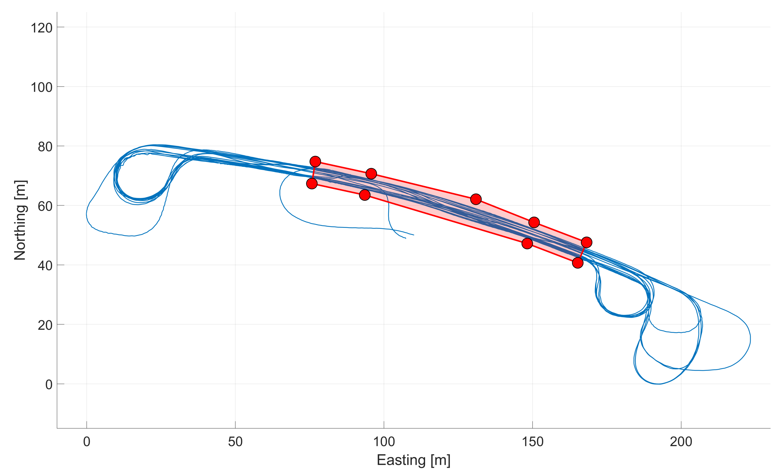
The LPS can be defined as a set of static nodes (i.e., infrastructure nodes) that are set up in the area of interest. These nodes enable the vehicle-to-infrastructure (V2I) terrestrial ranging and, consequently, the V2I positioning.
Ten infrastructure nodes were set up along the road. Every infrastructure node was equipped with a UWB TimeDomain (TD) unit, which enabled terrestrial ranging to the vehicles.
The coordinates of the infrastructure nodes were determined prior to the data collection based on the precise total station measurements with static GNSS observations.

3.2. Trajectory

During the data acquisition campaign, a few specific motion patterns were executed. Some of those patterns are: four vehicles moving in a platoon, vehicle pairs approaching road intersection, and then random motion of cyclist and/or pedestrian on the road and at the intersection. Figure 3 shows the platoon of four vehicles passing the intersection.
An example of the vehicle trajectories is shown in Figure 4 and Figure 5 (blue solid line). Infrastructure nodes are shown as red circles. The portion of the road around which the infrastructure nodes were set up will be addressed as main road area (Figure 5) in the following. In case of the unavailability of the GNSS data, in addition to V2V ranges, vehicles can rely on V2I ranges in the main road area. The results presented in Section 6 are based on the assumption of GNSS unavailability in the main road area in order to simulate the effect of loss of GNSS signal in a GNSS-denied environment.

3.3. Platform Setup

A different set of sensors was set up on each of the platforms, as shown in Table 1.
Each platform was equipped with a surveying grade GNSS receiver, except for GPSVan, which was equipped with two. The receivers acquired data for two purposes. First, they provided the reference trajectory (i.e., ground truth) for all the platforms. Second, the data were selectively used in the experiments. For example, mimicking a scenario when one or two platforms have good GPS data, while others have no data.
Two different UWB radios were used: 15 TimeDomain (TD) P410 and P440 (more about TD P440 at https://fccid.io/NUF-P440-A/User-Manual/User-Manual-2878444.pdf (accessed on 19 February 2021)) and 12 Pozyx (more about Pozyx at https://www.pozyx.io/documentation (accessed on 19 February 2021)) devices. As previously stated, every infrastructure node was equipped with a TD device. V2I ranging capability was enabled only for GPSVan. This means that an additional TD device was set up on the GPSVan to enable V2I ranging (denoted as TD V2I in Table 1). All platforms were equipped with a TD UWB device that enabled V2V ranging. Ranges between all vehicles are available, as well as ranges between GPSVan and the cyclist and the pedestrian. Pozyx devices were only used for V2V ranging. Every vehicle had two Pozyx radios installed (denoted as left (L) and right (R) in Table 1). Both TD V2V and Pozyx L and R were essential for implementing collaborative navigation in our experiments.
IMU data acquired on the GPSVan were used to create highly accurate ground truth trajectory, including position and attitude solutions.
Image data, both still imagery and video, were primarily acquired from the sensors mounted on the GPSVan with the goal of tracking other platforms. Figure 6 shows the positions of the cameras on the GPSVan: a GoPro camera (GPR1) and a Nikon were on the front of the vehicle, two Canons (CAN 1 and CAN 2) on the sides, and two Casios (CAS 1 and CAS 2) on the rear. The acquisition of the multiple image streams was uninterrupted. However, there is inherent uncertainty coming from the discontinuities in object tracking due to occlusions. The image sensor deployment on the GPSVan provides for 360 horizontal coverage around the vehicle.
Figure 7 shows the configuration of the sensors considered in this work for the GPSVan and other cars. Among all the available sensors and data, this paper will utilise data collected during a 40 min test by the following sensors:
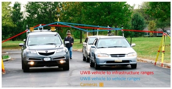
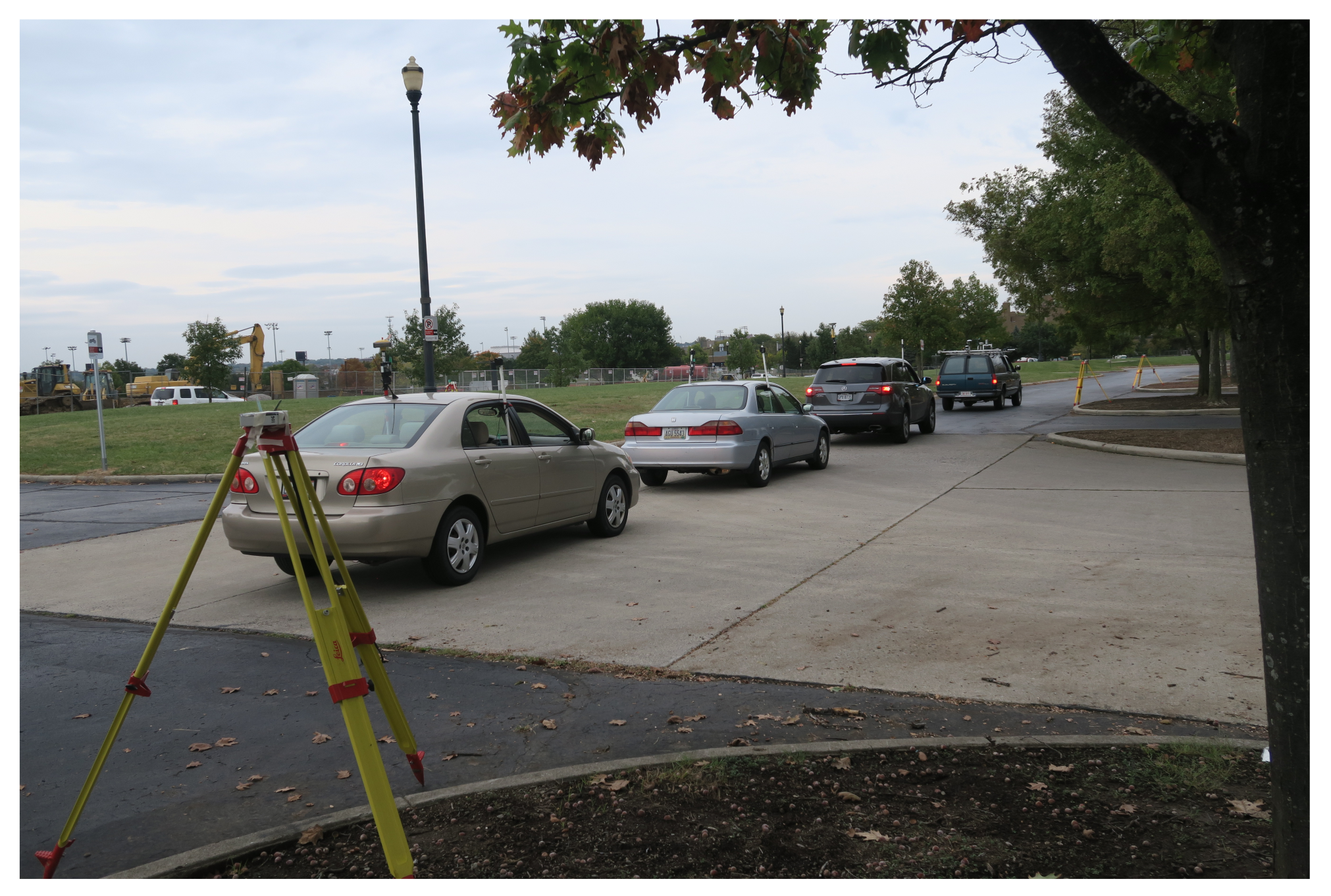
  • Sensors on the GPSVan: all UWB devices mounted on the vehicle, two GNSS receivers and one GoPro camera (GPR1).
  • Sensors on other cars: GNSS receiver, two Pozyx UWB devices (on the right and of the left of each vehicle), and one TimeDomain UWB transceiver.
  • Static network of 10 TimeDomain UWB transceivers.
Figure 7. Sensor setup.
Remotesensing 13 04858 g007
The GPSVan reference trajectory during the considered 40 min test is shown in Figure 5.

4. Data Characterisation

This section provides a description of the main sensor characteristics of the data that are used in the positioning algorithms discussed in Section 5.

4.1. TimeDomain Static UWB Network

The ten TimeDomain UWB anchors, shown in Figure 4, communicated with the rover V2I TimeDomain UWB (UWB200) mounted on the GPSVan. The rover checked range measurement availability from an anchor in approximately 0.032 s, and the average time period required to complete the polling of all anchors (i.e., to check again the measurement availability from the same anchor) was 0.32 s, as reported in the “V2I TD” column in Table 2. Given the presence of obstacles, or the relatively large distance between the UWB devices, the average measurement success rate (the number of received range measurements divided by the total number of checks done by the rover during all the tests, including when outside the main road area) is relatively low, at 13.4%.
Success rate is clearly much higher for short distances, as shown in Figure 8, Figure 9a and Figure 10a. Furthermore, Figure 8 shows that certain anchors (e.g., UWB204, which was the one more distant from the main road area) provided much fewer range measurements than others.
Despite the fact that ten anchors were available, the number of successful measurements in a rover check loop was larger than five only 1% of the time (Figure 11a).
Figure 11b shows the ranging error distribution, and Figure 10a the influence of distance on the error. In the box plot in Figure 10a, the central mark indicates the median error, the 25th and 75th percentiles are indicated by the bottom and top edges of the box, and the whiskers that extend to the most extreme data points are not considered outliers.
The results mentioned above were obtained after discarding unreliable measurements based on the QR index provided by TimeDomain devices, which allowed us to have only 1.8% of ranging errors larger than one meter (setting the threshold QR ≥ 60 cm, 3.1% of the measurements were discarded), as shown in Table 3.
Nevertheless, even exploiting the QR index for discarding unreliable measurements, a certain number of outliers are not detected; hence, it is suggested to use statistics to outliers to properly characterise the error, i.e., the median ranging error was −1 cm and median absolute deviation (MAD) was 18 cm (see Table 3).
Table 3 reports a detailed statistical characterisation of the ranging error:
  • Average error;
  • Median error;
  • Standard deviation of the error;
  • Median absolute deviation (MAD) = median ( | { e r } − median ( { e r } ) | ) ;
  • Median absolute error = i = 1 n | e r ( i ) | / n ;
  • Root mean square (RMS) error = i = 1 n e r ( i ) 2 / n ;
  • Percentage of errors larger than 1 m;
  • Percentage of unreliable measurements in accordance to the QR criteria, as mentioned above,
where e r ( i ) is the considered ranging error for the ith value of the time index, and n is the total number of considered instants.

4.2. TimeDomain V2V UWB Network

A V2V TimeDomain UWB device was mounted on each vehicle, as shown in Figure 7, and all of them communicated with each other and, in particular, with the rover V2V TimeDomain UWB (UWB300) mounted on the GPSVan. The rover checked range measurement availability from each car’s device in approximately 0.031 s, and the average time period required to complete the polling of all devices (i.e., to check again the measurement availability from the same couple of devices) was 0.24 s, as reported in the “V2V TD” column in Table 2. The average measurement success rate was 34.9%. Since all the V2V TimeDomain devices communicated with each other, potentially, up to six V2V range measurements could be measured at each polling loop.
Figure 9b shows the influence of distance on the measurement success rate, and Figure 10b shows that on the ranging error distribution. Then, Figure 12 compares the ranging error distribution for the distances between the GPSVan and the three cars.
Table 3 reports a detailed statistical characterisation of the ranging error. In particular, the median ranging error was −1 cm, and MAD was 45 cm.

4.3. Pozyx V2V UWB Network

Two V2V Pozyx UWB devices were mounted on each vehicle, as shown in Figure 7, divided in two networks, corresponding to the devices mounted on the right and on the left of the vehicles, respectively. The two networks worked on two different UWB channels (two and five), hence avoiding any interference between them. Each of the Pozyx UWB rovers mounted on the GPSVan checked range measurement availability from the devices in its own network in a loop. Since all the devices in a network communicated with each other, potentially, up to six V2V range measurements could be available for each network computation in every loop.
According to Table 2, each new measurement check was executed in approximately 0.018 s, and the average time period required to complete the loop (i.e., to check again the measurement availability from the same pair of devices) was 0.15–0.16 s, as reported in the “V2V Pozyx R” and “V2V Pozyx L” (R and L stand for right and left, respectively) columns in Table 2. The average measurement success rate was in the 31–39% range.
Figure 9c,d show the influence of distance on the measurement success rate, and Figure 10c,d show its influence on the ranging error distribution for the right and left network, respectively.
Then, Figure 13a shows the Pozyx ranging measurements between GPSVan and the Toyota car (right network measurements in yellow, left one in violet) compared to the corresponding GNSS-based distances between these two vehicles.
Figure 13b compares the ranging error distribution for the two Pozyx networks.
Table 3 reports a detailed statistical characterisation of the ranging error. In particular, median ranging error and MAD were 20 cm and 37 cm for the right network and 11 cm and 29 cm for the left one.

4.4. NLOS Detection and UWB Calibration

Table 3 shows that a relevant percentage of the UWB range observations are affected by quite large errors (larger than a meter), mostly due to the presence of obstacles in the considered scenario, such as metal surfaces causing reflections, resulting the acquisition of NLOS measurements. Consequently, the percentage is higher for V2V ranges, as both UWB transmitters used to measure a range are placed on vehicles, while for V2I, only one and the other UWB device was on a tripod, which is a benign environment.
Since the presence of NLOS measurements can have a negative impact on the accuracy of radio ranging-based methods, several methods have previously been investigated in the literature to detect NLOS ranges. In particular, three categories can be distinguished among NLOS detection methods, depending on if they are based on (i) range statistics, (ii) channel statistics, and (iii) positions [28]. Despite a significant number of recent works focused on (ii) [29,30], the prerequisite of (ii) is that the received signal is available, which makes it a non-viable option in this work. (iii) typically requires the presence of a redundant number of ranges from different devices in order to properly determine which ones are more reliable, and then leading, for instance, to a different weighting of the observations [31]. Hence, given the relatively low availability of simultaneous ranges (see, for instance, Figure 11a), in this study, a machine learning approach has been implemented for range-based NLOS detection.
To be more specific, random forest (RF) classifiers [32,33], trained on approximately a ten-minute dataset, have been used in order to detect NLOS UWB measurements, i.e., ranges with more than 1 m error. Since the characteristics of the UWB networks are slightly different, a specific classifier has been trained for each of them.
The estimates of the first, second, and third order temporal derivatives of the ranges have been considered inputs for the classifiers. Since there are some temporal gaps where observations are not available, such inputs are not always available, or not all of them are available. Hence, three different RF classifiers have been trained to allow NLOS detection when the following derivatives are available: (i) the first, (ii) the first and the second, or (iii) all of them. The first two lines of Table 4 show the percentage of measured data where it has been possible to run the RF classifiers according to this approach, and the obtained performance for such datasets (accuracy in detecting ranges with errors larger than 1 m). It is worth noting that the percentage of data examined by RF classifiers was lower for the TimeDomain devices due to the presence of more temporal gaps in the observation time series. The detection accuracy was above 94% for all the considered cases.
Then, the systematic component of the error has been partially compensated by assessing (on approximately a ten-minute dataset) and subtracting the median error for each pair of UWB devices. The use of more complex models of the UWB systematic error may also be considered (see, for instance, [1,34]). However, the dynamic scenario severely limits the potential advantages of more complex models. This aspect will be considered in our future investigations.
The error characteristics after NLOS removal by the RF classifiers and partial compensation of the systematic error components are shown in Table 4. The comparison between Table 3 and Table 4 shows that, despite the the fact that RF classifiers examined only around half the data in the TimeDomain case, the overall effect of the implemented approach is quite apparent, resulting in a remarkable reduction in the median error (in particular, in the Pozyx case) and its variability, as well as the presence of large errors. Given the high level of accuracy of all the RF classifiers, it is apparent that most of the remaining large errors are due to temporally quite isolated ranges, i.e., where derivatives could not be computed due to the temporal discontinuity of the signal.

4.5. GoPro Video

Among the cameras available on the GPSVan, this paper considers just the GPR1 camera shown in Figure 6. GPR1 is positioned on the front side of the GPSVan, and it approximately points in the heading direction of the vehicle, hence, in a quite convenient position and orientation to determine the angle between the vehicle heading and the cars in front of the GPSVan (see Figure 7).
GPR1 is a GoPro 5 Black camera, working in “Wide” field of view mode with a 3840 × 2160 resolution video at 30 Hz. Calibrated GPR1 camera parameters are assumed to be available in the following.

5. Positioning Approaches

In general, positioning methods assume that an accurate terrain model of the area is available. Considering an almost invariant height of the vehicles with respect to the ground, the 3D positioning problem can be reduced to 2D positioning.
In particular, the case study area considered in this work can be quite well approximated with a planar surface, whose normal changes approximately a 1 degree angle with respect to the vertical direction. Consequently, for the sake of notation simplicity, the positioning algorithms are formulated in the 2D case. Nevertheless, the generalization of such algorithms to the previously mentioned 3D case is trivial.
The next subsections provide details on the following implemented approaches:
  • V2I UWB positioning: vehicle position is estimated by exploiting only UWB range measurements with the static UWB infrastructure (Section 5.1).
  • Vision + UWB relative positioning: position of the other vehicles are computed by the GPSVan given the V2V UWB ranges and the visual information provided by the GoPro camera GPR1 (Section 5.2).
  • Cooperative positioning: vehicle position is estimated by exploiting V2V UWB range measurements, V2I measurements, visual information, and partial GPS/GNSS data (Section 5.3).
The V2I and cooperative positioning approaches described in the following subsections are based on the very common assumptions of Gaussian noise and linear approximation of the considered system; the prerequisites for using an extended Kalman filter (EKF). The reality, as shown in the previous subsection, is that the UWB ranging error in a realistic scenario has a light tail in the error distribution, typically caused by the presence of NLOS observations, which is only partially reduced by the implemented NLOS detection procedure. An in-depth investigation of the techniques to formally deal with non-Gaussian noise and different approximations of nonlinear system dynamics and measurement models is out of the scope of this work. The reader is referred to [35] for a recent investigation on these aspects in working conditions quite similar to those of this work.

5.1. V2I UWB Positioning

This subsection deals with the use of the ranging data between the static TD anchors and the TD device mounted on the GPSVan to assess its position. Since this subsection is mostly a standard implementation of the EKF [36,37,38], EKF experts may skip directly to the following subsection.
Let z k j be the range measurement between the GPSVan device and the j-th anchor, whose 2D position is p j = ( x j , y j ) , at the k-th iteration of the positioning algorithm. A timestamp t k j is typically collected along with the range z k j .
Additionally, let x k be the kth state vector, composed of the 2D vehicle position p ( t k ) = x t k , y t k and velocity v ( t k ) :
x k = p ( t k ) v ( t k )
To be specific, in this subsection, p ( t k ) refers to the position of the V2I TimeDomain rover (UWB300) mounted on the GPSVan. In certain cases, including the acceleration vector in the state can be convenient. Such generalisation is straightforward, and it is omitted here.
Then, the following dynamic model is used to describe the relation between x k and x k + 1 , i.e., the state evolution in Δ t k + 1 seconds:
x k + 1 = F k x k + ω k ,
where ω k is assumed to be a Gaussian-distributed zero-mean white noise process, with covariance matrix Q k , and F k is defined as follows:
F k = I Δ t k I 0 I
The measurement vector can be expressed as follows:
z k = z 1 j z k j ,
where the ranges in z k are those collected from the anchors during the kth measurement loop. Since anchors are sequentially checked, the ranges are collected at different times t k 1 , , t k j . Let t k , the time associated with x k , be equal to the average of t k 1 , , t k j (the approach can be easily extended to different choices of the t k value) and Δ t k = t k t k 1 . Furthermore, let δ t k j = t k j t k .
Then, the measurement model for z k j is
z k j = | p ( t k j ) p j | + ξ k = x t k j x j 2 + y t k j y j 2 + ξ k ,
where ξ k is assumed to be a Gaussian-distributed zero-mean white noise process, with variance σ ξ 2 . Since t k j t k , then, assuming a constant velocity in the ( t k , t k + t k j ) interval (the interval is written assuming t j j 0 , for simplicity of notation):
p ( t k j ) = p k + ( t k j t k ) v k = I δ t k j I x k
and
z k j = I δ t k j I x k p j + ξ k = h k j ( x k ) + ξ k
An extended Kalman filter approach is used to assess the state value x k , and in particular, the vehicle position, based on the available range measurements.
It is worth noting that, since range measurements are collected at different time instants, the vehicle may move meters between the first and last range measurements within a loop. Consequently, the innovation computation takes into account of such time differences and of the vehicle movement as follows:
ν k j = z k j z ^ k j ,
where ν k j is the jth component of the innovation vector,
z ^ k j = p k | k 1 j p j ;
p k | k 1 j = I δ t k j I x k | k 1 ;
x k | k 1 = F K 1 x k 1 | k 1 ,
where p k | k 1 j is the prediction of the vehicle position at time t j k , i.e., the prediction of p ( t k j ) , x k 1 | k 1 is the estimate of the state x k 1 given the measurements available up to the corresponding EKF iteration, whereas x k | k 1 is the prediction of the state vector x k given measurements available up to the previous iteration of the EKF. Furthermore, the row h k j , which is the one in the linearized observation matrix H k corresponding to the considered measurement z k j , is as follows:
h k j = p k | k 1 j p j z ^ k j δ t k j p k | k 1 j p j z ^ k j ,
which obtained linearizing (7) with respect to x k .

5.2. Relative Positioning with Vision and UWB
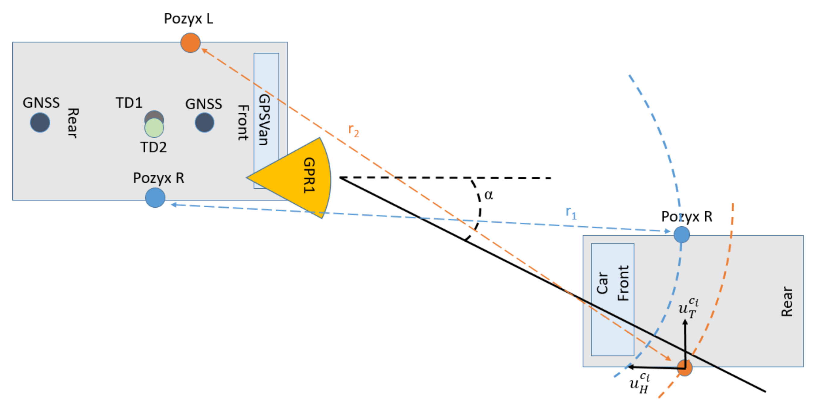
In this section, it is assumed that a vehicle c i is provided with a camera and UWB V2V ranging devices, which communicate with the UWB V2V devices mounted on the other vehicles. To be more specific, in this work, c i is the GPSVan, the considered camera is the GoPro camera, indicated as GPR1 in Figure 6, and the UWB V2V devices are those of the two Pozyx networks.
The approach presented in this subsection aims at combining vision and UWB V2V measurements to determine the relative positions of the other vehicles with respect to c i , i.e., with respect to the GPSVan.
To such aim, the first step is that of detecting the other vehicles in the GoPro video. This is achieved by exploiting a deep Learning car detection approach, and, in particular, a YOLO v3 network [39]. Fine tuning on approximately three hundred image samples of the vehicles was executed on a pre-trained YOLO v3 network in such a way to properly detect the cars involved in this test. Fully testing the YOLO v3 network is out of the scope of this paper; Figure 14 shows two examples of obtained car detection results.
For the simplicity of notation, the optical axis of the GPR1 camera is assumed to coincide with the GPSVan forward direction (see Figure 7), and the horizontal camera axis is assumed to lie on the horizontal plane. Furthermore, the camera is assumed to be perfectly modelled by the pinhole camera model (i.e., in practice, image coordinates are assumed to be already undistorted in the presentation below).
A bounding box is provided as output of the YOLO v3 Network when a vehicle is detected. Let α be the angle between the GPSVan forward direction and the line connecting the GoPro optical centre to the centre of the visible side of the detected car (Figure 7). Then, α can be assessed as follows:
α = arctan ( u b o x / f ) ,
where u b o x is the horizontal coordinate of the centre of the bounding box with respect to the optical centre, and f is the camera focal length, expressed in pixels. The error on the assessed value of α is assumed to be zero-mean and Gaussian, with standard deviation σ α .
Let, at least, a range measurement r 1 be available at time t between GPSVan and car c i , and assume that car c i is detected on the video frame acquired by GPR1 closest to time t. Since the GPR1 frame rate is 30 Hz (note that higher frame rates are available in recent video cameras), it is also assumed that the time difference between the video frame acquisition and t is negligible. Furthermore, let u α be the direction associated with such angle α . Then, the following steps can be distinguished in the implemented vision and UWB ranging positioning:
  • if just one UWB range measurement r 1 is available (assume, without loss of generalization, that r 1 is provided by the right Pozyx network), then the vehicle c i position is estimated as the intersection between the line passing through the GPR1 optical centre associated with the direction u α (black solid line in Figure 15) and the circumference associated with the r 1 range measurement (light blue dashed circumference in Figure 15);
  • if two UWB range measurements r 1 , r 2 are available, then the vehicle c i relative position with respect to the GPSVan is estimated along with the vehicle heading orientation by combining the three measurements. Let u H c i ( t k ) be car c i heading direction at time t k , and u T c i ( t k ) the corresponding transverse direction, then ( u T c i ( t k ) , u H c i ( t k ) ) define a car local reference system (see Figure 16). It is worth noting that u H c i ( t k ) can be uniquely identified in the 2D space by an angle θ , and that once u H c i ( t k ) is known, then u T c i ( t k ) is uniquely determined as well. Assume also that the relative position of the two Pozyx devices is known in the car local reference system. Then, vehicle relative position p r c i and orientation with respect to the GPSVan are determined by solving the following optimisation problem:
    { p ^ r c i , θ ^ } = arg min p r c i , θ r 1 r ^ 1 p r c i , θ ^ 2 σ r 1 2 + r 2 r ^ 2 p r c i , θ ^ 2 σ r 2 2 + α α ^ p r c i , θ ^ 2 σ α 2 ,
    where r ^ 1 , r ^ 2 , and θ ^ are the distances between the Pozyx devices in the two cars and the c i orientation according to the estimated position. The solution of such optimisation problem can be quickly obtained by means of the Gauss–Newton algorithm, where the stopping condition can be set imposing a threshold on the computed solution variation (only up to the millimetre level for what concerns the variation on the estimated position).
Then, the absolute position of car c i can be easily obtained from the relative one p ^ r c i if the absolute position and orientation of the GPSVan are available.

5.3. Cooperative Positioning

This subsection describes the combined use of GPS/GNSS, UWB V2I, and V2V measurements and vision in a centralised cooperative positioning approach. For simplicity of notation, in this subsection, t k is assumed to be coincident to one of the possible GNSS measurement time instants, and Δ t k = 0.2 s.
In the proposed centralised approach, the state vector is formed by joining the state vectors of all the considered cars, which are four in this work. Without loss of generality, hereafter, equations will be reported assuming the use of just four cars. Nevertheless, the generalisation to a generic number of vehicles is trivial.
Similarly to Section 5.1, an EKF is used to obtain reliable state estimates; however, the approach presented in Section 5.1 shall be slightly generalised to deal with several vehicles and different sensor measurements.
Hereafter, the position of the ith car is conventionally defined as the position of the GNSS receiver mounted on such vehicle. For the GPSVan, the vehicle position is defined as the GNSS antenna on the rear side of the vehicle.
Let p c i ( t ) and v c i ( t ) be the position and velocity of the ith car at time t, respectively, and, with a slight abuse of notation, let x k be the joint state vector at time t k and x k c i the state part corresponding to the ith car, which can be defined as in (1). Then,
x k = x k c 1 x k c 4
The state dynamic model is as in (2); however, F k is redefined as follows:
F k = F k 0 0 0 0 F k 0 0 0 0 F k 0 0 0 0 F k ,
where F k corresponds to the single car transition matrix, which is defined as in (3).
Differently from Section 5.1, the observation vector z k can now be decomposed in four different types of measurements:
z k = z k G N S S z k V 2 I z k V 2 V z k v i s
The measurement model is as follows:
z k = h k ( x k ) + ξ k
where, similarly to z k , three components can be distinguished in h k ( · ) as well:
h k ( x k ) = h k G N S S ( x k ) h k V 2 I ( x k ) h k V 2 V ( x k ) h k v i s ( x k ) ,
where h k G N S S ( x k ) is related to the GPS/GNSS position measurements, when available. Assuming, for simplicity of notation, that GNSS is available for all the vehicles, then
h k G N S S ( x k ) = I 0 x k c 1 I 0 x k c 4
When GNSS measurement is unavailable at time t k for car i, then the ith line of the above matrix shall be discarded.
Let the GPSVan correspond to car 1, and let ( Δ p T V 2 I , Δ p H V 2 I ) be the displacement of TD200 with respect to the rear GNSS receiver in the GPSVan. Since the V2I network communicated only with TD200, mounted on the GPSVan, then h k V 2 I ( x k ) can be easily derived from (7):
h k V 2 I ( x k ) = | p k c 1 , V 2 I ( δ k 1 ) p 1 | | p k c 1 , V 2 I ( δ k j ) p j | ,
where it is assumed that V2I measurements from all anchors are available, and, assuming constant velocity in a short time interval centred in t k , p k c 1 , V 2 I ( δ k j ) is the position of TD200 at the time of the ranging measurement with anchor j:
p k c 1 , V 2 I ( δ k j ) = p k c 1 + δ k j v k c 1 + u T c 1 ( t k ) Δ p T V 2 I + u H c 1 ( t k ) Δ p H V 2 I
When the measurement from the jth anchor is not available at time t k , then the jth row in (21) shall be discarded.
h k V 2 V ( x k ) refers to the V2V range measurements. For simplicity of notation, assume that only one V2V UWB device is mounted on each vehicle, and let ( Δ p T i , Δ p H i ) be its displacement with respect to the GNSS receiver on such vehicle. Furthermore, let t k + δ t k i i be the time instant of the ranging measurement between vehicle i and i . Then, h k V 2 V ( x k ) can be expressed as follows:
h k V 2 V ( x k ) = | p k c 1 , V 2 V ( δ k 12 ) p k c 2 , V 2 V ( δ k 12 ) | | p k c i , V 2 V ( δ k i i ) p k c i , V 2 V ( δ k i i ) | ,
where it is assumed that V2V measurements from all anchors are available, and, assuming constant velocity in a short time interval centred in t k , p k c i , V 2 I ( δ k i i ) , the position at time t k + δ k i i of the V2V UWB device on car i with respect to the GNSS receiver is:
p k c i , V 2 V ( δ k i i ) = p k c i + δ k i i v k c i + u T c i ( t k ) Δ p T i + u H c i ( t k ) Δ p H i
When the range measurement between car i and i is not available, then the corresponding row in (23) shall be discarded.
Finally, the vision information, when available, is assumed to be integrated with UWB as described in Section 5.2. Let the vision measurements be provided at time t k + δ k v i s , and let Δ p k c i , v i s ( δ k v i s ) be the relative position of car c i with respect to the GPSVan at such time instant (assuming for simplicity of notation that the vehicle position for the vision approach in Section 5.2 is coincident with the one used here); then, when all the cars are detected on a frame:
h k v i s ( x k ) = Δ p k c 2 , v i s ( δ k v i s ) Δ p k c i , v i s ( δ k v i s )
When the measurement of car i is not available, then the corresponding line in (25) shall be discarded.
Then, the linearized observation matrix H k , assuming for simplicity all the measurements available, can be expressed as follows:
H k = I 0 0 0 0 0 I 0 0 0 I 0 0 0 0 0 0 0 I 0 h ¯ k 1 0 0 h ¯ k 10 0 0 h k c 1 , c 2 h k c 2 , c 1 0 0 h k c 1 , c 3 0 h k c 3 , c 1 0 0 0 h k c 5 , c 6 h k c 6 , c 5 h k c 2 , v i s , 1 h k c 2 , v i s , 2 0 0 h k c 3 , v i s , 1 0 h k c 3 , v i s , 2 0 h k c 4 , v i s , 1 0 0 h k c 4 , v i s , 2 ,
where the computation of h ¯ k j , h k c i , c i , h k c i , v i s , 1 , and h k c i , v i s , 2 shall linearize the corresponding terms in h k V 2 I , h k V 2 V , and h k v i s . It is worth noting that u H c i ( t k ) (and, consequently, u T c i ( t k ) ) is usually expected to be correlated with the velocity vector of the ith vehicle. Nevertheless, hereafter, their estimation is assumed to be done by means of a separate procedure, independent of the positioning presented here. For instance, exploiting IMU measurements: vehicle orientation can be assessed by properly combining gyroscope, magnetometer, and acceleration measurements, e.g., GPSVan heading direction in the considered dataset can be computed even only exploiting magnetometer data, obtaining a zero-mean approximately Gaussian angle error, with standard deviation 3.5 deg. As a consequence of this observation, h ¯ k j can be computed similarly to h k j :
h ¯ k j = p k | k 1 c 1 , V 2 I p j z ^ k j δ t k j p k | k 1 c 1 , V 2 I p j z ^ k j ,
where, similarly to (10), p k | k 1 c 1 , V 2 I is the prediction of p k c 1 , V 2 I ( δ t k j ) given the state value at time t k 1 , and z ^ k j is the predicted distance between the GPSVan and the jth V2I anchor.
Then, let p k | k 1 c i be the prediction of p k c i , V 2 I ( δ t k i i ) given the state value at time t k 1 , and z ^ k i , i be the predicted distance at time t k + δ t k i i between vehicle i and i .
h ¯ k c i , c i = p k | k 1 c i p k | k 1 c i z ^ k i , i δ t k j p k | k 1 c i p k | k 1 c i z ^ k i , i
p k | k 1 c 1 , V 2 I and p k | k 1 c i can be easily obtained from (22) and (24), respectively, using the portions of the predicted state value corresponding to p k c i and v k c i .
Finally, under the assumption that the vehicle orientation is available, h k c i , v i s , 1 and h k c i , v i s , 2 can be simply written as h k c i , v i s , 1 = p k | k 1 c 1 , v i s , h k c i , v i s , 2 = p k | k 1 c i , v i s , where p k | k 1 c i , v i s is the prediction of the car c i position at time t k + δ k v i s .

6. Results and Discussion

The positioning results obtained using the algorithms presented in the previous section are analyzed in the following subsections. The performance of all the algorithms is evaluated on the main road area (see Figure 5), where vehicle GNSS measurements are assumed to be either completely or only partially unavailable/unreliable (e.g., such as in a urban canyon). All the positioning algorithms have been implemented in Matlab and executed in post-processing on a Pentium i7-6700HQ CPU with 16GB of RAM. The analysis of the computational complexity of the proposed approaches is out of the scope of this work. Nevertheless, since the maximum execution time in the considered simulations is around 0.6 s for each minute of collected data, these computations could have been run in real-time on any mid-range CPU.

6.1. Positioning with a Static UWB Infrastructure (V2I)

GPSVan 2D positioning error, based on the use of V2I infrastructure as described in Section 5.1, is shown in Figure 17. The positioning performance on the main road area is much better than that on the overall area, as expected. In particular, the median value of the 2D positioning error is 15 cm on the main road area, with MAD = 35 cm, as reported in Table 5. A more careful analysis of the 2D positioning error shows that its distribution along the vehicle heading direction (“main road along track” in Table 5) and along its orthogonal direction (“main road across-track” in Table 5) is quite similar.

6.2. Relative Positioning with Vision and UWB

The results of this subsection aim at validating the performance of the approach described in Section 5.2 to assess the relative position between cars. More specifically, a 10 min video collected by the GoPro GPR1 (see Figure 6 and Figure 7) during the experiment was analysed. Since the information provided by successive frames is quite correlated, the frames to be processed were extracted from the video at 10 Hz.
The obtained 2D relative positioning error and its characteristics along the GPSVan heading direction and its orthogonal are reported in Table 6. According to Table 6 and Figure 18a, the 2D error is typically less than 1 m and slightly larger in the direction orthogonal to the vehicle motion.
It is worth noting that the angular error, due to the vision-based car detection, plays an important role in the overall 2D positioning error. Indeed, the 2D positioning error is clearly correlated with the absolute value of the angular error, as shown in Figure 18b.
Despite the approximately zero-mean and unimodal angular error distribution, most of the errors are in the ( 2 , + 2 ) interval, as shown in Figure 19a; the largest errors are more than 10 degrees. Such errors are usually caused by imprecise detection boxes; the YOLO v3 network occasionally associates with a detected vehicle a box remarkably larger than the real car area, as shown, for instance, in Figure 19b.

6.3. Cooperative Positioning

The performance of the approach described in Section 5.3 is tested considering different case studies, such as varying the availability of the UWB, vision, and GNSS measurements.
In particular, the following cases are considered:
  • V2I: positioning obtained by considering only UWB V2I measurements. Since V2I measurements are available only for the GPSVan (here and in all the cases where they are used), positions of all the other cars inside the main road area are obtained just as Kalman predictions from the last available GNSS measurements, i.e., their trajectories will be straight lines until GNSS updates are available.
  • V2I + V2V cooperative approach: cooperative positioning obtained by considering UWB V2I and V2V measurements.
  • V2I + V2V + vision cooperative approach: cooperative positioning obtained by considering UWB V2I and V2V measurements and the information coming from the vision based relative positioning system.
  • V2I + V2V + partial random GNSS availability: cooperative positioning obtained by considering UWB V2I and V2V measurements and a certain percentage of GNSS measurements randomly available in the main road area (car and time instant of any available measurement are randomly selected). The percentage of available GNSS measurements varies from 0.5% to 4%.
  • V2V + GNSS available on certain vehicles: cooperative positioning obtained by considering all UWB V2V measurements and GNSS measurements available on certain cars, varying the number of cars from 1 to 3.
Table 7 shows the relative distance error between all the vehicles for the V2I and the V2I+V2V cases. For what concerns the latter, the last two columns also show the relative distance error restricted to the time instants when all cars receive UWB range measurements from at least n c vehicles, for n c = { 2 , 3 } . The mean absolute distance error is lower than 1 m in all the cases exploiting V2V measurements, being 24 cm in good V2V communication conditions, i.e., when n c = 3 .
Table 8 reports the 2D cooperative positioning error for three cars (V2I + V2V case), excluding GPSVan, whose position is, in practice, derived by the V2I measurements (see Table 5). The last two columns also consider the effect of introducing vision in the positioning algorithm.
It is worth noting that, since V2I measurements are available only for the GPSVan, the main effect of V2I is that of enabling the estimation of the GPSVan position, whereas the positions of the other cars with respect to the GPSVan can only be assessed when V2V (and vision, when considered) measurements are available.
Table 8 shows that the cooperative positioning approach has clear advantage from being in good V2V communication conditions ( n c = 3 ); indeed, the V2I + V2V median error and MAD decrease from 2.4 m and 3.2 m to 2.0 m and 2.0 m, and in the vision case, they decrease from 2.3 m and 2.0 m to 1.5 m and 1.6 m. The latter results also show the improvement in the positioning performance obtained thanks to vision.
Figure 20 shows the 2D positioning error of the cars (excluding GPSVan) as a function of the GNSS outage time, comparing the performance of the V2I + V2V and of the V2I + V2V + vision approach in the time interval corresponding to the 10 min video of the GoPro GPR1. Dashed lines show the median 2D positioning error, whereas the shadowed error bars show the 25% and 75% percentile of the error distribution.
Figure 21 shows a short portion of the tracks of the four vehicles during the test, as an example. In this example the four vehicles are moving in two opposite directions: GPSVan and Toyota from left to right of Figure 21, whereas Acura and Honda from right to left. Then, Figure 22 shows the car positions in four successive time instants ( t i at the ith row of the figure, with t i < t i + 1 ), extracted from those shown in Figure 21, estimated by means of the V2I + V2V approach (column (b)) and of the V2I + V2V + vision approach (column (c)), compared with the reference (GNSS-based) solution (column (a)). Solid black lines connecting vehicles are shown when the corresponding UWB V2V range measurements are available. Both Figure 20 and Figure 22 confirm the positive impact of vision on the cooperative positioning performance.
The influence of partial random availability of GNSS on the cooperative positioning performance is assessed in Table 9. Table 9 reports the 2D positioning error for three cars, excluding GPSVan, throughout the 40-min test while varying, from 0.5% to 4%, the percentage of randomly available GNSS measurements on the cars in the main road area. In order to make the results statistically more robust, the results shown in the table were obtained from 100 independent Monte Carlo simulations.
Furthermore, Table 10 restricts the analysis of the positioning performance of the cooperative approach, focusing only on the Monte Carlo results on the time instants with UWB range measurements for all cars from n c = 3 vehicles.
In good V2V working conditions ( n c = 3 ), the availability of just 0.5% of the GNSS measurements allows us to reduce the median positioning error from 2.0 m to 1.5 m and the mean absolute error from 3.0 m to 2.8 m (compare the “V2I + V2V ( n c = 3 )” column in Table 8 with the 0.5% column in Table 10). The performance clearly improves with increasing the availability of GNSS measurements, reaching a median error of 0.5 m and mean absolute error of 0.7 m in the 4% case.
Figure 23 shows the 2D positioning error of the cars (excluding GPSVan) as a function of the GNSS outage time, varying the percentage of available GNSS measurements, from 0.5% to 4%, in the Monte Carlo simulations. Dashed lines show the median 2D positioning error, whereas the shadowed error bars show the 25% and 75% percentile of the median error distribution over the 100 Monte Carlo simulations.
Finally, the performance of the cooperative positioning algorithm is tested when varying the number of vehicles n G that have (full) access to the GNSS measurements in the main road area. Four cases are distinguished:
  • V2I + V2V: GPSVan is provided with UWB V2I measurements, whereas all the other cars can only exploit UWB V2V measurements to determine their positions.
  • V2V + ( n G = 1 ): GPSVan is provided with GNSS measurements, whereas all the other cars can only exploit UWB V2V measurements to determine their positions.
  • V2V + ( n G = 2 ): GPSVan and Honda are provided with GNSS measurements, whereas the other cars can only exploit UWB V2V measurements to determine their positions.
  • V2V + ( n G = 3 ): GPSVan, Honda, and Acura are provided with GNSS measurements, whereas Toyota can only exploit UWB V2V measurements to determine its position.
It is worth noting that the reliability of the cooperative positioning solution depends on the vehicle geometric configuration, on the available UWB measurements, and on the specific car trajectory. Hence, in order to make a fair comparison between the four cases listed above, the results reported in Table 11 consider only the 2D positioning error of the Toyota car.
Then, Table 12 also shows the Toyota 2D positioning error, restricting the analysis only to the time instants with UWB range measurements received from all vehicles ( n c = 3 ).
The performance of V2I + V2V and V2V + ( n G = 1 ) are quite similar in both Table 11 and Table 12. Furthermore, the performance of the last two cases ( n G = 2 and n G = 3 ) are quite similar. In good V2V working conditions ( n c = 3 ), the availability of good positioning information on at least two vehicles ( n G 2 ) allows us to obtain a quite dramatic improvement in the positioning error, e.g., median error reduces from 3.7 m to 0.8 m.
To conclude, Figure 24 shows a portion of the tracks of the four vehicles during the test, as an example. In this example, the four vehicles are moving in the same direction (from left to right of Figure 24), but on two different lanes; GPSVan on the left lane, and Acura, Honda, and Toyota in line on the right lane. Then, Figure 25 shows the car positions in three successive time instants ( t i at the ith row of the figure, with t i < t i + 1 ), extracted from those shown in Figure 24, estimated by the V2I + V2V approach (column (b)) and the V2I + V2V + ( n G = 2 ) (column (c)), compared with the reference (GNSS-based) solution (column (a)). Solid black lines connecting vehicles are shown when the corresponding UWB V2V range measurements are available. Figure 25 confirms the positioning performance improvement that is typically obtained when n G 2 .

6.4. Discussion

UWB data characterisation in Section 4 showed that the average ranging success rate for all the UWB networks is lower than 40% (Table 2), with a clear dependence of the success rate on the distance between the UWB devices (Figure 9).
While the ranging success rate of all the UWB networks decreases at larger distances, the distance at which the success rate becomes lower than 10% is quite different: 40 m and 80 m for the TimeDomain V2I and V2V networks, and 45 m and 30 m for the right and left Pozyx networks, the success range of the latter being generally lower than the TimeDomain one for distances larger than 30 m. The different performance of TimeDomain V2I and V2V networks is probably due to the different chance of obstructions along the line-of-sight between the UWB devices, whereas the different behavior between the two Pozyx networks, whose devices are mounted on the two sides of the same vehicles, is probably also due to the different transmission channels.
A consequence of the above observation is the low availability of UWB ranges in a measurement loop period: the maximum number of UWB range measurements available in a loop depends on the number of devices in the network (i.e., 10 in the V2I case, 6 for the V2V); however, during the test, each network rarely measured more than four ranges (e.g., Figure 11a), hence implying a lower robustness of the real UWB network geometry configuration in the positioning algorithm with respect to its potential one (given by all the UWB devices used in the test).
The UWB ranging error is at decimeter level for both Pozyx and TimeDomain devices (Table 3), despite being remarkably worse in the Pozyx case, in particular, for its systematic component, i.e., median error quite different from zero. The impact of the distance between the UWB devices on the ranging accuracy appears quite moderate in the experimental results (Figure 10). Instead, the presence of NLOS measurements have occasionally affected the ranging error, causing the presence of outliers (and, more generally, a lighter tail in the ranging error distribution, as is visible in Figure 12 and Figure 13b). Nevertheless, outliers were remarkably more frequent in the range measurements of the Pozyx networks than in the TimeDomain ones, probably also thanks to the use of the QR index to discard unreliable measurements in the TimeDomain devices. Again, the different performance of TimeDomain V2I and V2V networks (larger error dispersion in the V2V case) is probably due to the different chance of NLOS measurements.
The use of RF classifiers proved to be quite effective to detect NLOS observations when temporal continuity of the ranging is guaranteed, e.g., classifier accuracy ≥ 94.1%, as shown in Table 4. However, a remarkable number of large UWB errors occurred when ranging temporal continuity was not ensured, hence causing an only partial reduction of the NLOS observations thanks to the implemented RF-based method.
Overall, the obtained UWB ranging results are consistent with the nominal technical specifications of such devices. However, given the quite low ranging success rate for distances larger than 30–45 m, it is worth noting that this kind of technology is quite ineffective for localization purposes when the UWB devices are far from each other. Nevertheless, determining the relative distance and position between cars is clearly much more important for short distances between them.
A confirmation of the correctness of the above consideration is also given by the performance results shown in Table 5 and Figure 17 for the V2I-based positioning case (Section 5.1); the positioning performance of the GPSVan, the only vehicle provided with V2I measurements, on the main road area (i.e., in the area where anchors were deployed) is much better than that on the overall area. Despite the fact that the median error on the all areas is quite similar to the one on the main road, this is mainly due to the fact that the vehicles mostly moved in the main road area. Actually, the dispersion of the error is much larger in the all test area (MAD > 2 m). Restricting the analysis to the main road, the accuracy of the obtained 2D positioning error is at sub-meter level (median value of 12 cm, MAD = 31 cm). The error distribution along the travel and lateral direction is quite similar, being slightly larger on the latter one, probably due to the anchor network configuration with respect to the vehicle track.
It is worth noting that, even if the average UWB measurement sample period is around few tens of milliseconds for all the UWB networks, the average ranging loop period is in the ( 0.15, 0.32) s interval, which caused the need of taking into account of the car movement during such time interval in the positioning algorithm (Section 5).
The combined use of UWB V2V ranges and vision, based on the use of the GoPro GPR1 mounted on the front of the GPSVan (Figure 7), for relative positioning (Section 5.2) showed to be quite effective, with 2D error at sub-meter level both along the heading direction and its transverse (Table 6 and Figure 18a). The angular error, shown in Figure 19a, due to the vision-based car detection, plays an important role in the overall 2D positioning error, as proved by the correlation between the relative positioning error and the absolute value of the angular error in Figure 18b. An improvement of the car detection precision of the implemented YOLO v3 network (an example of a quite large error is shown in Figure 19b) shall be considered in our future work in order to reduce the influence of the above mentioned angular error on the 2D relative positioning error. The introduction in our approach of the use of external physical objects/features (e.g,. people, traffic lights) visible by several vehicles will also be considered in our future investigations [40].
For what concerns the results of the cooperative positioning, some observations are now in order:
  • First, the results reported in Table 7 show that the use of UWB V2V measurements allowed to assess car relative distances with an uncertainty approximately at meter level. Instead, the car relative distance assessment reached an uncertainty at decimeter level when ranges from at least other two cars are available on all the vehicles ( n c 2 ). Hence, in such working conditions, the relative distance between cars can be quite effectively assessed.
  • The first goal of Table 8 is that of evaluating the collaborative positioning performance of the V2I + V2V approach: the obtained 2D positioning error is at meter level (median = 2.4 m, MAD = 3.2 m), with a quite clear improvement when working in good V2V measurement conditions, i.e., median error = 2.0 m, MAD = 2.0 m when n c = 3 . The positioning error increases with the outage time (see Figure 20a), as expected. The median error is lower than 2 m for approximately 8 s of outage. It is worth noting that V2I ranges were available only for the GPSVan; hence, V2I enables computing the absolute positioning of the GPSVan, whereas the positions of the other cars can be assessed only through the V2V measurements.
  • Then, Table 8 and Figure 20b show that the introduction of vision in the positioning algorithm can reduce the error (median = 2.3 m, MAD = 2.0 m) and its increase with the outage time (the median error is lower than 2 m for approximately 12 s of outage). Similarly to the V2I + V2V case, the positioning error is reduced when working in good V2V measurement conditions: median error = 1.5 m, MAD = 1.6 m, when n c = 3 . Since video frames have currently been extracted from the video (and processed) at 10 Hz, processing them at the original video frame rate is expected to improve the overall positioning results.
  • Figure 22 shows an example of the (b) V2I + V2V and (c) V2I + V2V + vision performance on a portion of the car tracks, to be compared with (a) the reference one. By comparing the car positions in (b) with those in (a), it is quite apparent that the relative distances between cars are quite consistent with the correct ones when the corresponding range measurements are available, as expected. However, since only the GPSVan absolute position can be assessed (from the V2I ranges), the absolute positioning problem for the other cars is ill posed. Let us consider the static positioning problem on a certain time instant: any rotation, pivoting on the GPSVan, of the real car configuration is equally acceptable. Instead, since the vision-aided solution includes also some (indirect) information on the car configuration orientation (i.e., the angle α in Figure 7), such solution is less prone to the above mentioned ill-posedness.
  • The above considerations suggest that, in order to avoid ill-posed solutions in the UWB-based cooperative positioning, either some information shall be provided by external sensors (e.g., vision), or more than one vehicle shall be provided with measurements to enable absolute positioning, e.g., V2I measurements.
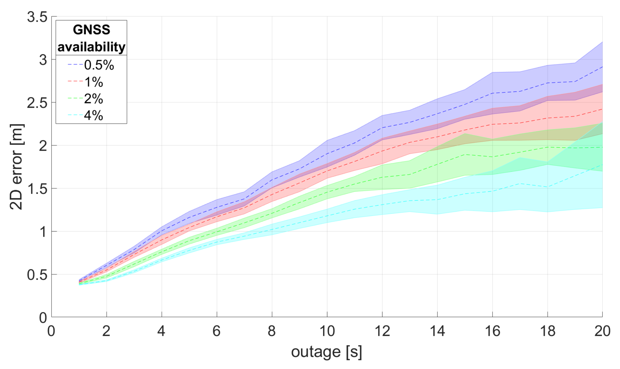
  • The results reported in Table 9 aim at investigating the absolute positioning performance that can be achieved when GNSS is partially available in the main road area. In particular, the performance is evaluated varying the percentage of available GNSS measurements. Comparing the results of Table 9 with those of Table 10, it is quite apparent the importance of the availability of a sufficient number of successful V2V range measurements in order to effectively propagate to the other vehicles the information provided by the few available GNSS positions. In particular, the results obtained when n c = 3 (Table 10) with a certain amount of GNSS measurements are similar to those obtained in Table 9, doubling the percentage of GNSS measurements. Overall, the obtained positioning error is at meter level, reaching sub-meter level in good working conditions for the V2V communications and with 4% of the GNSS measurements (last column in Table 10). The median error is usually lower than 2 m for more than 20 outage seconds when at least 2% of the GNSS measurements are available, as shown in Figure 23. These results confirm that the use of a cooperative approach and an effective V2V ranging system can reduce the need for GNSS measurements when aiming at meter/sub-meter positioning of groups of vehicles.
  • The comparison between the results in the first two columns of Table 11 and Table 12 shows that the positioning performance of the cooperative positioning approach (on the cars provided only with V2V measurements) is quite similar when exploiting UWB V2I or GNSS on the GPSVan.
  • Finally, the last three columns of Table 11 and Table 12 aim at evaluating the performance of the cooperative positioning (evaluated on the same car, e.g., Toyota) when varying the number of vehicles n G provided with GNSS measurements in the main road area. The obtained results show a significant improvement when increasing n G from 1 to 2, whereas the difference between n G = 2 and 3 is quite modest. Similarly to the previously considered cases, Table 12 confirms that good V2V ranging is very important for the efficiency of the cooperative approach, as expected. Furthermore, Figure 25 shows that, despite the fact that n G = 2 is not sufficient for theoretically ensuring to avoid ill-posedness of the positioning solution, it is enough to avoid it in the considered example and in most real-world scenarios as well.
To summarize, when UWB measurements are available, they can be considered quite reliable and useful for determining the distances between vehicles and their relative positions. Machine learning tools, such as random forest, can be used to reduce the NLOS UWB observations. The V2I approach ensured positioning accuracy at sub-meter level, whereas quite solid results, with error at meter level, have been obtained in the V2V case for n c = 3 in most of the considered scenarios. To be more specific, since n c 2 is usually sufficient to ensure the assessment of relative car distances at sub-meter level of accuracy, n c = 3 is just required to ensure the solution to be robust against rotations. Furthermore, the V2V-based positioning also requires a certain number of vehicles to be provided of quite good absolute positioning data (e.g., V2I or GNSS) in order to properly avoid ill-posedness of the overall solution. Vision also showed to be useful, both to obtain quite decent positioning results when combined with UWB ranging and to reduce the chance of ill-posed solutions. Overall, the combination of UWB and vision seems to be quite promising, despite the quite limited measurement success rate of UWB for ranges larger than some tens of meters imposes some limits on their usability.

7. Conclusions

Despite the fact that GNSS is currently used for positioning and navigation by billions of devices all over the world, its use is still challenging in certain working conditions, such as indoors, in urban canyons, in tunnels. In order to compensate the unavailability (or unreliability) of GNSS in such working conditions, this paper investigated the performance of UWB-based cooperative vehicle positioning. The rationale of cooperative positioning is that sharing navigation data by a group of vehicles can improve vehicle navigation compared to the individual solutions.
The sine qua non working condition for cooperative positioning is the availability of range measurements between the vehicles, and the connectivity between them in order to share such information. In our experiments, we mostly focused on the V2I and V2V communication cases, with ranging data provided by UWB transceivers. Additionally, an initial investigation on the feasibility of integrating UWB with vision has also been conducted by considering the data fusion between UWB and a camera mounted on one of vehicles in our test, namely the GPSVan.
UWB data characterization showed that both systems used in this work can ensure ranging accuracy at decimeter level, which is consistent with their nominal characteristics and with the objectives of this work. Nevertheless, despite the fact that the maximum range of the two systems were around 100 m or more, the measurement success rate remarkably decreased over 30–45 m, resulting in occasional gaps in the measurements. This aspect is a critical factor for the system, imposing a limitation on its usability; the UWB-based cooperative positioning approach can be considered reliable only when vehicles are quite close to each other. Nevertheless, this operating condition is clearly of major interest in real scenarios. The presence of NLOS observations is one of the principal factors causing a decrease in the UWB ranging performance; however, machine learning tools, such as random forest classifiers, showed to be useful to effectively detect NLOS observations.
The experimental results show that a V2I UWB infrastructure can be effectively implemented to obtain 2D positioning accuracy at sub-meter level when GNSS is not available.
However, since the V2I approach is effective only in the area covered by a quite dense network of UWB static anchors, the installation of this kind of infrastructure on a large area can be quite expensive. Then, V2V measurements have been employed in order to investigate the possibility of reducing the need of such a dense V2I UWB infrastructure. The test results show that UWB-based V2V ranging can reliably assess the relative car distances at sub-meter level of accuracy, in particular, when a sufficient number of ranges are available ( n c 2 ), i.e., when the vehicles are quite close to each other.
In our experiment with four cars, at least two vehicles shall be provided of good absolute positioning data, e.g., V2I or GNSS measurements, in order to properly use V2V to enable the assessment of the absolute positions of the other vehicles, avoiding ill-posedness of the solution. The use of UWB V2I and GNSS to assess the absolute position of certain vehicles led to quite similar results when introducing such information in the V2V cooperative positioning approach, with a V2V positioning accuracy at meter level (with n c = 3 ). Since n c 2 usually ensures relative car distance results quite similar to n c = 3 , n c = 3 is just required to guarantee the solution to be robust against rotations.
The integration of UWB with vision led to quite good relative positioning results (sub-meter level of accuracy) and to an improvement in the cooperative approach results in terms of absolute positioning, but still at meter level of accuracy. On the positive side, the use of vision also relaxes the above mentioned requirement of having at least two vehicles with good positioning data.
Overall, the obtained results showed that, when good V2V communications are ensured, typically, meter or sub-meter accuracies can be achieved, which can be considered quite adequate along the travel direction.
In our future work, it is foreseen, in particular, to improve the integration between UWB and vision, processing the visual information at a higher rate, improving the vehicle detection approach, and considering a larger number of cameras: such changes are expected to have a quite positive impact on the positioning results. The study of an optimal strategy for properly sizing V2I and V2V communications will also be considered, taking into account both the infrastructure cost and the risk of packet collisions under quite dense traffic conditions [41]. Finally, a more in depth investigation is also foreseen on the assessment of integrity, continuity, and availability of the cooperative positioning solution.

Author Contributions

Conceptualization, A.M., C.T., J.G., G.R., A.K., H.P. and V.G.; methodology, A.M.; software, A.M.; validation, A.M.; formal analysis, A.M.; investigation, A.M.; data curation, A.M.; data collection A.M., C.T., J.G., G.R., H.P. and V.G.; writing—original draft preparation, A.M., C.T., J.G., G.R. and A.K.; writing—review and editing, all authors; visualization, A.M., C.T. and J.G.; resources, A.M., C.T., A.K. and V.G.; supervision, C.T., A.K. and V.G. All authors have read and agreed to the published version of the manuscript.

Funding

No external funding is reported for this paper.

Conflicts of Interest

The authors declare no conflict of interest.

References

  1. Retscher, G.; Kealy, A.; Gabela, J.; Li, Y.; Goel, S.; Toth, C.K.; Masiero, A.; Błaszczak-Bąk, W.; Gikas, V.; Perakis, H.; et al. A benchmarking measurement campaign in GNSS-denied/challenged indoor/outdoor and transitional environments. J. Appl. Geod. 2020, 14, 215–229. [Google Scholar] [CrossRef]
  2. Li, Y.; Williams, S.; Moran, B.; Kealy, A.; Retscher, G. High-dimensional probabilistic fingerprinting in wireless sensor networks based on a multivariate Gaussian mixture model. Sensors 2018, 18, 2602. [Google Scholar] [CrossRef] [PubMed] [Green Version]
  3. Shan, J.; Toth, C. Topographic Laser Ranging and Scanning: Principles and Processing; CRC Press: Boca Raton, FL, USA, 2018. [Google Scholar] [CrossRef]
  4. Shen, F.; Cheong, J.W.; Dempster, A.G. A DSRC Doppler/IMU/GNSS tightly-coupled cooperative positioning method for relative positioning in VANETs. J. Navig. 2017, 70, 120–136. [Google Scholar] [CrossRef] [Green Version]
  5. Petovello, M.G.; O’Keefe, K.; Chan, B.; Spiller, S.; Pedrosa, C.; Basnayake, C. Demonstration of inter-vehicle UWB ranging to augment DGPS for improved relative positioning. In Proceedings of the 23rd International Technical Meeting of the Satellite Division of The Institute of Navigation (ION GNSS 2010), Portland, OR, USA, 21–24 September 2010; pp. 1198–1209. [Google Scholar]
  6. Adegoke, E.I.; Zidane, J.; Kampert, E.; Ford, C.R.; Birrell, S.A.; Higgins, M.D. Infrastructure Wi-Fi for connected autonomous vehicle positioning: A review of the state-of-the-art. Veh. Commun. 2019, 20, 100185. [Google Scholar] [CrossRef] [Green Version]
  7. Zampella, F.; Ruiz, A.R.J.; Granja, F.S. Indoor positioning using efficient map matching, RSS measurements, and an improved motion model. IEEE Trans. Veh. Technol. 2015, 64, 1304–1317. [Google Scholar] [CrossRef]
  8. Li, X.; Wang, Y.; Liu, D. Research on extended Kalman filter and particle filter combinational algorithm in UWB and foot-mounted IMU fusion positioning. Mob. Inf. Syst. 2018, 2018, 215–229. [Google Scholar] [CrossRef]
  9. Retscher, G.; Gikas, V.; Hofer, H.; Perakis, H.; Kealy, A. Range validation of UWB and Wi-Fi for integrated indoor positioning. Appl. Geomat. 2019, 11, 187–195. [Google Scholar] [CrossRef] [Green Version]
  10. Toth, C.K.; Jozkow, G.; Koppanyi, Z.; Grejner-Brzezinska, D. Positioning slow-moving platforms by UWB technology in GPS-challenged areas. J. Surv. Eng. 2017, 143, 04017011. [Google Scholar] [CrossRef]
  11. Kurazume, R.; Nagata, S.; Hirose, S. Cooperative positioning with multiple robots. In Proceedings of the 1994 IEEE International Conference on Robotics and Automation, San Diego, CA, USA, 8–13 May 1994; pp. 1250–1257. [Google Scholar]
  12. Grejner-Brzezinska, D.A.; Toth, C.K.; Moore, T.; Raquet, J.F.; Miller, M.M.; Kealy, A. Multisensor navigation systems: A remedy for GNSS vulnerabilities? Proc. IEEE 2016, 104, 1339–1353. [Google Scholar] [CrossRef]
  13. De Ponte Müller, F. Survey on ranging sensors and cooperative techniques for relative positioning of vehicles. Sensors 2017, 17, 271. [Google Scholar] [CrossRef] [Green Version]
  14. Fascista, A.; Ciccarese, G.; Coluccia, A.; Ricci, G. Angle of Arrival-Based Cooperative Positioning for Smart Vehicles. IEEE Trans. Intell. Transp. Syst. 2018, 19, 2880–2892. [Google Scholar] [CrossRef]
  15. Dressler, F.; Hartenstein, H.; Altintas, O.; Tonguz, O.K. Inter-vehicle communication: Quo vadis. IEEE Commun. Mag. 2014, 52, 170–177. [Google Scholar] [CrossRef]
  16. Amini, A.; Vaghefi, R.M.; Jesus, M.; Buehrer, R.M. Improving GPS-based vehicle positioning for intelligent transportation systems. In Proceedings of the 2014 IEEE Intelligent Vehicles Symposium Proceedings, Dearborn, MI, USA, 8–11 June 2014; pp. 1023–1029. [Google Scholar]
  17. Mohammadmoradi, H.; Heydariaan, M.; Gnawali, O. SRAC: Simultaneous ranging and communication in UWB networks. In Proceedings of the 2019 15th International Conference on Distributed Computing in Sensor Systems (DCOSS), Santorini Island, Greece, 29–31 May 2019; pp. 9–16. [Google Scholar]
  18. Alam, N.; Dempster, A.G. Cooperative Positioning for Vehicular Networks: Facts and Future. IEEE Trans. Intell. Transp. Syst. 2013, 14, 1708–1717. [Google Scholar] [CrossRef]
  19. Wang, D.; O’Keefe, K.; Petovello, M. Decentralized cooperative positioning for vehicle-to-vehicle (V2V) application using GPS integrated with UWB range. In Proceedings of the ION 2013 Pacific PNT Meeting, Honolulu, HI, USA, 23–25 April 2013; pp. 793–803. [Google Scholar]
  20. Ćesić, J.; Marković, I.; Cvišić, I.; Petrović, I. Radar and stereo vision fusion for multitarget tracking on the special Euclidean group. Robot. Auton. Syst. 2016, 83, 338–348. [Google Scholar] [CrossRef]
  21. Bombini, L.; Cerri, P.; Medici, P.; Alessandretti, G. Radar-vision fusion for vehicle detection. In Proceedings of the International Workshop on Intelligent Transportation, Toronto, ON, Canada, 17–20 September 2006; Volume 65, p. 70. [Google Scholar]
  22. Wang, X.; Xu, L.; Sun, H.; Xin, J.; Zheng, N. On-Road Vehicle Detection and Tracking Using MMW Radar and Monovision Fusion. IEEE Trans. Intell. Transp. Syst. 2016, 17, 2075–2084. [Google Scholar] [CrossRef]
  23. Mahlisch, M.; Schweiger, R.; Ritter, W.; Dietmayer, K. Sensorfusion using spatio-temporal aligned video and lidar for improved vehicle detection. In Proceedings of the 2006 IEEE Intelligent Vehicles Symposium, Meguro-Ku, Japan, 3–15 June 2006; pp. 424–429. [Google Scholar]
  24. Roeckl, M.; Gacnik, J.; Schomerus, J.; Strang, T.; Kranz, M. Sensing the environment for future driver assistance combining autonomous and cooperative appliances. In Proceedings of the Fourth International Workshop on Vehicle-to-Vehicle Communications (V2VCOM), Eindhoven, The Netherlands, 3 June 2008; pp. 45–56. [Google Scholar]
  25. Rockl, M.; Frank, K.; Strang, T.; Kranz, M.; Gacnik, J.; Schomerus, J. Hybrid fusion approach combining autonomous and cooperative detection and ranging methods for situation-aware driver assistance systems. In Proceedings of the 2008 IEEE 19th International Symposium on Personal, Indoor and Mobile Radio Communications, Cannes, France, 31 August–4 September 2008; pp. 1–5. [Google Scholar]
  26. De Ponte Müller, F.; Diaz, E.M.; Rashdan, I. Cooperative positioning and radar sensor fusion for relative localization of vehicles. In Proceedings of the 2016 IEEE Intelligent Vehicles Symposium (IV), Gotenburg, Sweden, 19–22 June 2016; pp. 1060–1065. [Google Scholar]
  27. Fujii, S.; Fujita, A.; Umedu, T.; Kaneda, S.; Yamaguchi, H.; Higashino, T.; Takai, M. Cooperative vehicle positioning via V2V communications and onboard sensors. In Proceedings of the 2011 IEEE Vehicular Technology Conference (VTC Fall), San Francisco, CA, USA, 5–8 September 2011; pp. 1–5. [Google Scholar]
  28. Khodjaev, J.; Park, Y.; Malik, A.S. Survey of NLOS identification and error mitigation problems in UWB-based positioning algorithms for dense environments. Ann. Telecommun.-Ann. Des Télécommun. 2010, 65, 301–311. [Google Scholar] [CrossRef]
  29. Yu, K.; Wen, K.; Li, Y.; Zhang, S.; Zhang, K. A novel NLOS mitigation algorithm for UWB localization in harsh indoor environments. IEEE Trans. Veh. Technol. 2018, 68, 686–699. [Google Scholar] [CrossRef]
  30. Yang, X. NLOS mitigation for UWB localization based on sparse pseudo-input Gaussian process. IEEE Sens. J. 2018, 18, 4311–4316. [Google Scholar] [CrossRef]
  31. Pointon, H.A.; McLoughlin, B.J.; Matthews, C.; Bezombes, F.A. Towards a model based sensor measurement variance input for extended Kalman filter state estimation. Drones 2019, 3, 19. [Google Scholar] [CrossRef] [Green Version]
  32. Pal, M. Random forest classifier for remote sensing classification. Int. J. Remote Sens. 2005, 26, 217–222. [Google Scholar] [CrossRef]
  33. Biau, G.; Scornet, E. A random forest guided tour. TEST 2016, 25, 197–227. [Google Scholar] [CrossRef] [Green Version]
  34. Perakis, H.; Gikas, V. Evaluation of Range Error Calibration Models for Indoor UWB Positioning Applications. In Proceedings of the 2018 International Conference on Indoor Positioning and Indoor Navigation (IPIN), Nantes, France, 24–27 September 2018; pp. 206–212. [Google Scholar]
  35. Gabela, J.; Kealy, A.; Li, S.; Hedley, M.; Moran, W.; Ni, W.; Williams, S. The effect of linear approximation and Gaussian noise assumption in multi-sensor positioning through experimental evaluation. IEEE Sens. J. 2019, 19, 10719–10727. [Google Scholar] [CrossRef]
  36. Anderson, B.D.; Moore, J.B. Optimal Filtering; Prentice-Hall: Englewood Cliffs, NJ, USA, 2012. [Google Scholar]
  37. Jazwinski, A.H. Stochastic Processes and Filtering Theory; Academic Press: New York, NY, USA; London, UK, 2007. [Google Scholar]
  38. Kailath, T.; Sayed, A.; Hassibi, B. Linear Estimation; Prentice-Hall: Englewood Cliffs, NJ, USA, 2000. [Google Scholar]
  39. Redmon, J.; Farhadi, A. YOLOv3: An Incremental Improvement. arXiv 2018, arXiv:1804.02767. [Google Scholar]
  40. Soatti, G.; Nicoli, M.; Garcia, N.; Denis, B.; Raulefs, R.; Wymeersch, H. Implicit cooperative positioning in vehicular networks. IEEE Trans. Intell. Transp. Syst. 2018, 19, 3964–3980. [Google Scholar] [CrossRef] [Green Version]
  41. Yao, J.; Balaei, A.T.; Hassan, M.; Alam, N.; Dempster, A.G. Improving cooperative positioning for vehicular networks. IEEE Trans. Veh. Technol. 2011, 60, 2810–2823. [Google Scholar] [CrossRef] [Green Version]
Figure 1. A group of four vehicles equipped with GPS/GNSS, UWB, IMU and camera sensors. Red lines show 3 out of the 6 inter-vehicle ranges (V2V), blue lines show 4 ranges from 2 infrastructure points to 3 vehicles (V2I), and dashed lines show GPS/GNSS signals; note that not all signal receptions are shown.
Remotesensing 13 04858 g001
Figure 2. Four vehicles, bicycle and pedestrian platforms used in the experiments with the network of infrastructure nodes.
Remotesensing 13 04858 g002
Figure 3. Four vehicles moving as a platoon.
Remotesensing 13 04858 g003
Figure 4. Typical drive pattern of vehicles (blue track) and TimeDomain UWB anchors (circular red marks).
Remotesensing 13 04858 g004
Figure 5. Main road area (red) and GPS Van reference trajectory (blue).
Remotesensing 13 04858 g005
Figure 6. Camera installation on the GPSVan.
Remotesensing 13 04858 g006
Figure 8. TimeDomain UWB static network: Comparing UWB ranging with distance computed using GPSVan reference trajectory for two different anchors, namely UWB204 (a) and UWB102 (b).
Remotesensing 13 04858 g008
Figure 9. Influence of distance on the UWB measurement success rate. UWB networks: (a) TimeDomain V2I static network, (b) TimeDomain V2V network, (c) Pozyx V2V right network, (d) Pozyx V2V left network.
Remotesensing 13 04858 g009
Figure 10. Influence of distance on the UWB error. UWB networks: (a) TimeDomain V2I static network, (b) TimeDomain V2V network, (c) Pozyx V2V right network, (d) Pozyx V2V left network.
Remotesensing 13 04858 g010
Figure 11. TimeDomain UWB static network: (a) number of simultaneously available range measurements, (b) ranging error distribution.
Remotesensing 13 04858 g011
Figure 12. TimeDomain UWB V2V network: ranging error distribution of the TimeDomain rover mounted on the GPSVan with those on the other three vehicles.
Remotesensing 13 04858 g012
Figure 13. Pozyx UWB V2V ranging. (a) Comparing UWB ranging with distance computed using GNSS trajectories for GPSVan−Toyota, (b) ranging error distribution: left (violet) and right (yellow) net.
Remotesensing 13 04858 g013
Figure 14. Examples of car detection in the GoPro video: (a) Acura SUV and (b) Toyota Corolla detected in two different frames.
Remotesensing 13 04858 g014
Figure 15. Vision + UWB positioning with one UWB range measurement.
Remotesensing 13 04858 g015
Figure 16. Vision + UWB positioning with two UWB range measurements.
Remotesensing 13 04858 g016
Figure 17. TimeDomain UWB V2I positioning: 2D error on GPSVan positioning.
Remotesensing 13 04858 g017
Figure 18. (a) 2D positioning error obtained combining vision with UWB and decomposition of such error along the GPSVan heading direction and its orthogonal one. (b) Relation between the 2D positioning error and the vision−based angle measurement error.
Remotesensing 13 04858 g018
Figure 19. (a) Distribution ofthe vision−based angular measurement error [deg]. (b) Example of vehicle with associated detection box larger than expected.
Remotesensing 13 04858 g019
Figure 20. (a) 2D positioning error as a function of the outage time. Comparison between: (a) UWB V2I + V2V and (b) UWB V2I + V2V + vision approaches.
Remotesensing 13 04858 g020
Figure 21. Example: four vehicles divided in two groups moving in the main road area in opposite directions.
Remotesensing 13 04858 g021
Figure 22. Positioning results in four successive time instants ( t 1 , , t 4 ) during the example of Figure 21: ith row of the figure corresponds to time instant t i . Comparison of different approaches: (a) GNSS (reference), (b) UWB V2I + V2V, (c) UWB V2I + V2V + vision.
Remotesensing 13 04858 g022
Figure 23. 2D positioning error as a function of the outage time. Comparison between the performance obtained in 100 Monte Carlo simulations varying, from 0.5% to 4%, the percentage of available GNSS measurements in the main road area.
Remotesensing 13 04858 g023
Figure 24. Example: four vehicles moving in the main road area in the same direction on two different lanes.
Remotesensing 13 04858 g024
Figure 25. Positioning results in three successive time instants ( t 1 , , t 3 ) during the example of Figure 24: ith row of the figure corresponds to time instant t i . Comparison of different approaches: (a) GNSS (reference), (b) UWB V2I + V2V, (c) UWB V2I + V2V + ( n G = 2 ).
Remotesensing 13 04858 g025
Table 1. Sensors used on test platforms.
PlatformsGPSTD V2ITD V2VPozyx-LPozyx-RIMUCamera
GPSVan, reference vehicleXXXXXXX
Honda AccordX XXX
Acura SUVX XXX
Toyota CorollaX XXX
BicycleX X
PedestrianX X XX
Table 2. UWB ranging characterization.
V2I TDV2V TDV2V Pozyx RV2V Pozyx L
Avg. measurement sample period [s]0.0320.0310.0180.018
Avg. ranging loop period [s]0.320.240.160.15
Avg. success rate [%]13.434.939.031.3
Max. range [m]9616813973
Table 3. UWB ranging error.
V2I TDV2V TDV2V Pozyx RV2V Pozyx L
Average [cm]612715
Median [cm]−1−12011
Stand. dev. [cm]741087069
MAD [cm]18453729
Mean. Abs. err. [cm]17414130
RMS [cm]741097571
Max [m]13213946
% | err . | 1  m1.86.49.64.3
% unreliable ranges (QR)3.16.0
Table 4. RF performance and calibrated UWB ranging error.
V2I TDV2V TDV2V Pozyx RV2V Pozyx L
Data examined by RF (%)60.844.789.688.3
RF accuracy (%)99.697.694.196.7
Median [cm]0022
MAD [cm]13363327
Mean. Abs. err. [cm]12343227
RMS [cm]61886768
% | err . | 1  m1.45.25.83.4
Table 5. GPSVan V2I positioning: 2D error.
All AreaMain RoadMain Road
Along Track
Main Road
Across-Track
Median [cm]16122−3
MAD [cm]268311521
Mean. Abs. err. [cm]182301521
RMS [cm]764733663
% | err . | 2  m13.33.12.74.6
Table 6. Vision + UWB 2D positioning error and its directional characteristics.
2D ErrorHeadingTransverse
Median [cm]2412−11
MAD [cm]502637
Mean. Abs. err. [cm]533139
RMS [cm]915870
% | err . | 1  m16.78.911.0
Table 7. Cooperative positioning: car relative distance error.
V2IV2I + V2VV2I + V2V
( n c 2 )
V2I + V2V
( n c = 3 )
Median [m]0.00.000.000.00
MAD [m]16.00.800.300.24
Mean. Abs. err. [m]11.50.790.300.24
RMS [m]34.22.360.520.41
Table 8. Cooperative positioning: 2D positioning error, excluding GPSVan.
V2IV2I + V2VV2I + V2V
( n c = 3 )
V2I + V2V +
Vision
V2I + V2V +
Vision
( n c = 3 )
Median [m]13.42.42.02.31.5
MAD [m]33.63.22.02.01.6
Mean. Abs. err. [m]31.24.23.03.12.4
RMS [m]61.75.94.04.23.3
Table 9. Cooperative positioning: 2D positioning error, excluding GPSVan, varying the percentage of GNSS measurements available in the main road area.
0.5%1%2%4%
Median [m]2.11.40.90.6
MAD [m]4.12.81.70.9
Mean. Abs. err. [m]4.53.11.91.1
RMS [m]8.15.93.71.9
Table 10. Cooperative positioning: 2D positioning error, excluding GPSVan, varying the percentage of GNSS measurements available in the main road area, restricted only to time instants when cars received V2V measurements from all vehicles ( n c = 3 ).
0.5%1%2%4%
Median [m]1.51.00.70.5
MAD [m]2.41.50.80.5
Mean. Abs. err. [m]2.81.81.10.7
RMS [m]4.63.01.71.0
Table 11. Cooperative positioning: Toyota 2D positioning error varying the number of cars n G provided with GNSS measurements in the main road area.
V2I + V2VV2V + ( n G = 1 ) V2V + ( n G = 2 ) V2V + ( n G = 3 )
Median [m]4.03.71.21.2
MAD [m]6.65.53.62.9
Mean. Abs. err. [m]7.76.63.53.0
RMS [m]12.811.58.55.9
Table 12. Cooperative positioning: Toyota 2D positioning error varying the number of cars n G provided with GNSS measurements in the main road area, restricted only to time instants when Toyota received V2V measurements from all cars.
V2I + V2VV2V + ( n G = 1 )V2V + ( n G = 2 )V2V + ( n G = 3 )
( n c = 3 )( n c = 3 )( n c = 3 )( n c = 3 )
Median [m]4.03.70.80.8
MAD [m]4.44.31.20.9
Mean. Abs. err. [m]6.05.51.51.2
RMS [m]8.37.62.72.2
Publisher’s Note: MDPI stays neutral with regard to jurisdictional claims in published maps and institutional affiliations.

