Thermographic Monitoring of Scum Accumulation beneath Floating Covers

Abstract

Large sheets of high-density polyethene geomembrane are used as floating covers on some of the wastewater treatment lagoons at the Melbourne Water Corporation’s Western Treatment Plant. These covers provide an airtight seal for the anaerobic digestion of sewage and allow for harvesting the methane-rich biogas, which is then used to generate electricity. There is a potential for scum to develop under the covers during the anaerobic digestion of the raw sewage by microorganisms. Due to the nature of the operating environment of the lagoons and the vast size (450 m × 170 m) of these covers, a safe non-contact method to monitor the development and movement of the scum is preferred. This paper explores the potential of using a new thermographic approach to identify and monitor the scum under the covers. The approach exploits naturally occurring variations in solar intensity as a trigger for generating a transient thermal response that is then fitted to an exponential decay law to determine a cooling constant. This approach is investigated experimentally using a laboratory-scale test rig. A finite element (FE) model is constructed and shown to reliably predict the experimentally observed thermal transients and cooling constants. This FE model is then set up to simulate progressive scum accumulation with time, using a specified scumberg geometry and a stepwise change in thermal properties. The results indicate a detectable change in the cooling constant at different locations on the cover, thereby providing a quantitative basis for characterising the scum accumulation beneath the cover. The practical application and limitations of these results are briefly discussed.

1. Introduction

Geomembranes have been extensively used in several applications, such as landfill liner systems [1,2], water reservoirs [3] and mining facilities [4], to assist with the degradation of wastes, protect groundwater, provide a barrier to stop the diffusion of contaminants, contain or harvest gaseous emissions, or a combination of any of these. High-density polyethylene (HDPE) is one of the most widely adopted materials for geomembranes due to its high crystallinity, which results in high stiffness and tensile strength, as well as good chemical stability. It is also known as a durable material with highly desirable long-term performance. The expected service life of the HDPE geomembrane is reported to be more than 150 years at an operating temperature of 35 °C [5]. The Melbourne Water Corporation (MWC) uses large floating covers made from multiple sheets of HDPE for the wastewater treatment lagoons at its Western Treatment Plant (WTP) in Werribee, Australia. The purpose of these covers, spanning an area of 450 × 170 m², as shown in Figure 1, is (i) to provide an airtight seal for the anaerobic digestion of raw sewage (ii) to harvest the methane-rich biogas generated by this anaerobic digestion as a renewable resource for electricity generation and (iii) to prevent the release of odorous and greenhouse gases into the environment. Under peak operating conditions, each floating cover can harvest up to 65,000 m³ of biogas per day, which is sufficient to generate 7 MW of electricity energy [6,7,8]. This renewable energy is used for operational requirements at the WTP, with excess electricity exported to the grid to offset usage at other MWC sites.

Raw sewage flows into the lagoons at the covered end, and partially treated effluent leaves at the other end for the next stage of processing, while under the cover, fibrous materials, fats, floating solids and buoyed sludge contained in the raw sewage may combine to form a semi-solid scum that has the potential to accumulate at the underside of the cover. The progressive accumulation of semi-solid scum may lead to the formation of solid scum or large scumbergs, whose impact may include either or both of (1) impeding the biogas collection pathways beneath the cover, thereby reducing the harvesting efficiency, and hence the renewable energy generation, and (2) lifting the geomembrane covers above the surface level of the sewage in the lagoons by up to 1 m, thus producing a “whaleback” region that is susceptible to drag forces induced by inflow or strong winds, which may impact the structural integrity of the covers. This paper investigates the potential of a novel thermographic technique for detecting and monitoring the semi-solid and solid scum under the floating covers at the WTP. The main aim of this paper is to provide a preliminary assessment of a novel quasi-active thermographic approach [9,10,11] as a quantitative methodology to classify the state of scum formation.

The current practice at the WTP to establish the extent and state of the scum beneath the cover involves walk-the-cover inspections that deliver a qualitative assessment of the state and extent of the scum based on the to-the-foot feel. This is supported by the manual insertion of sticks in the inspection holes in the cover to estimate scum depth. The state of scum is qualitatively (and subjectively) assessed as “hard”, “medium”, “soft” and “fluffy”. This form of assessment needs to be improved for effective asset management. Hence, it is preferable to develop a quantitative method that also does not require personnel to “work on water”.

Thermal imaging is one of the most extensively deployed remote sensing methods for monitoring large structures. Omar and Nehdi [12,13] mounted a thermal camera on an unmanned aerial vehicle (UAV) to scan the temperature distribution on the deck of a bridge. Thermal imaging has also been used to measure the temperature of buildings [14,15], concrete structures [16] and aircraft structures [17,18]. In our previous work [19,20,21], a UAV was deployed to measure the surface elevation of the floating covers at the WTP. This approach can be adapted to also include thermal imaging. However, in contrast to conventional thermography, which relies on the temperature contrast within a single frame of a thermal image, this work explores the use of a cooling constant derived from Newton’s law of cooling for the purpose of monitoring the state and extent of scum accumulation. Newton’s law of cooling describes the cooling process of objects that have higher temperature than ambient. According to Newton’s law of cooling, the rate of temperature reduction of an object is governed by the cooling constant. In the convection cooling process, the cooling constant can be used to estimate how fast the temperature of the object decreased to the ambient temperature [9,10,11].

This paper is organised into two parts. In the first part, experimental measurements of the cooling constant are undertaken on a rooftop test rig, using naturally occurring variations in the daily solar intensity as the trigger for thermal transients. A finite element (FE) model of the test rig is constructed, using as inputs the experimentally measured values of solar intensity and ambient temperature. It is shown that the FE model predictions of the thermal transients agree well with the experimental measurements, thereby validating the FE methodology. In the second part, this validated FE methodology is used to investigate the variation in the cooling constant due to a progressive change in the thermal properties of simulated scum, and the implications of the results for practical implementation are discussed.

2. Methodology

2.1. Experimental Setup

A laboratory-scale experiment was set up within an open space on an exposed roof-top to simulate the anaerobic lagoons at the WTP. Figure 2 shows a 1 m × 0.5 m segment of 2-mm-thick HDPE geomembrane, representative of the floating covers at the WTP, which has been deployed across part of an aluminium tray. The edges of the HDPE geomembrane were clamped to the perimeter of the tray by aluminium frames. To simulate the effect of solid scum under the cover, a portion of the tray was filled with clayey soil. The membrane was then installed over the tray, with some regions that were in contact with the clayey soil and other regions that were suspended over the air (referred to as the “no-soil” region).

The incident solar intensity and the ambient temperature were recorded with an Apogee SP-110 pyranometer [22] and a Fluke 287 thermal probe that were deployed alongside the test apparatus, as shown in Figure 3, for the entire 1-day experiment. Technical specifications of the pyranometer and the multi-meter are listed in

Table 1. Manufacture data of the Apogee SP-110 pyranometer.

Technical Data	Specification
Sensitivity	0.2 mV/Wm−2
Output range	0–400 mV
Field of view (FOV)	180 o
Mass	90 g
Operating temperature	−40–70 °C
Response time	<1 ms

and

Table 2. Manufacture data of the thermal probe.

Technical Data	Specification
Instrument model	Fluke 287 thermal probe
Operating temperature	−20 °C–55 °C
Mass	871 g
Temperature resolution	0.1 °C
Accuracy	±1%

, respectively. A FLIR A615 infrared thermal camera [23] was set up alongside the HDPE geomembrane to synchronously measure the surface temperature (see Figure 3). The technical specifications of the thermal camera are listed in

Table 3. Manufacturer data of the FLIR A615 IR camera.

Technical Data	Specification
IR resolution	640 × 480 pixels
FOV	25° × 19°
Minimum focus distance	0.25 m
Accuracy	±2 °C
Frame rate	3–50 Hz
Noise-equivalent temperature difference (NETD)	<0.05 °C @ +30 °C (+86 °F)/50 mK
Spectral range	7.5–14 μm
Operating temperature	−40 °C–150 °C
Detector type	Focal plane array (uncooled microbolometer)

.

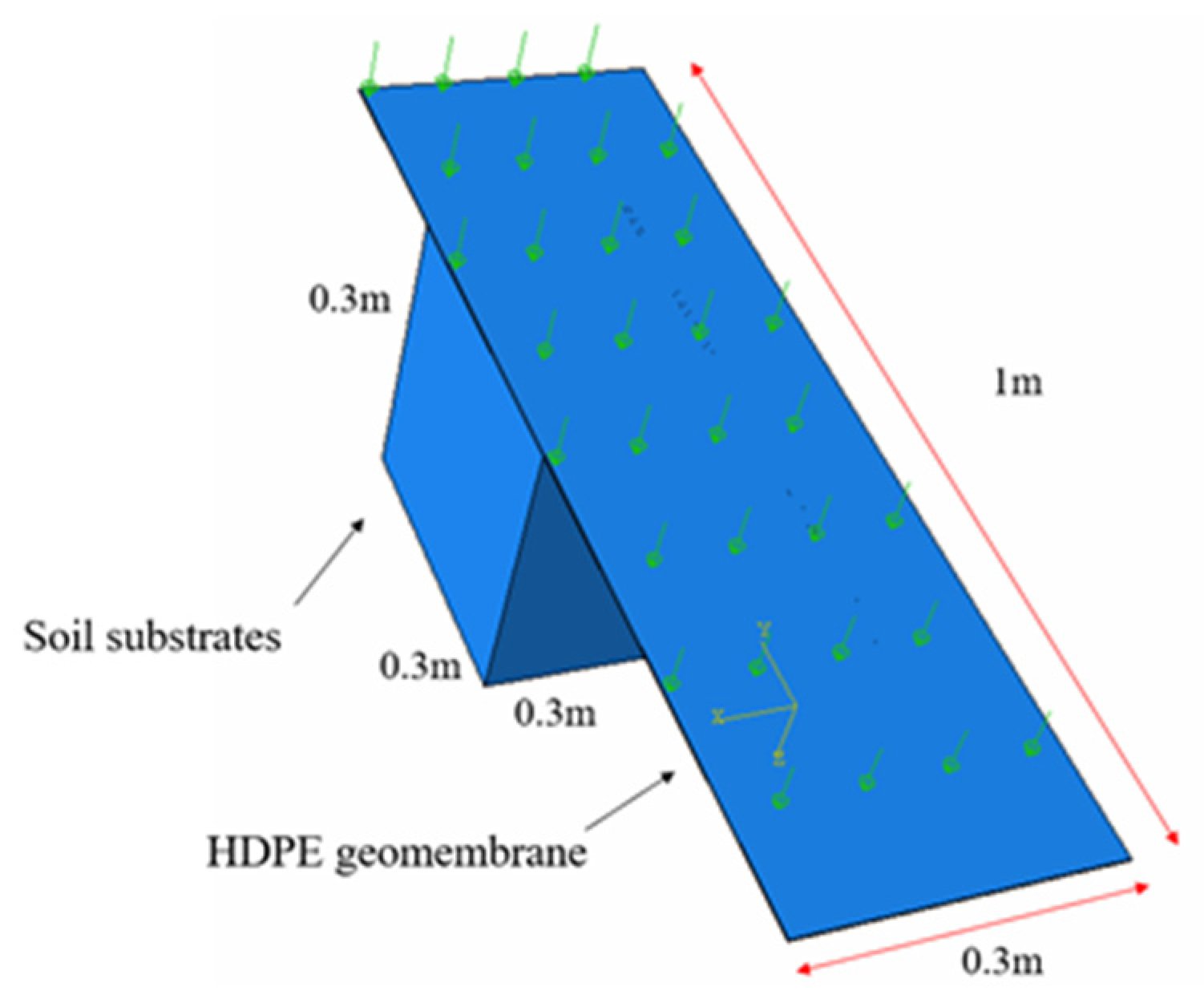
2.2. Finite Element Model

A finite element (FE) model of the experimental setup was constructed within the commercial package ABAQUS [24], based on the geometry shown in Figure 4 and the model details in

Table 4. FE model details.

Model Data	Specification
Membrane size	2 mm × 0.3 m × 1 m
Soil substrate size	0.3 m × 0.3 m × 0.3 m
Model type	3-D deformable solid
Element type	DCC3D8: an 8-node convection/diffusion brick element (heat transfer element)
Element shape	Hex
Element size	1 mm

.

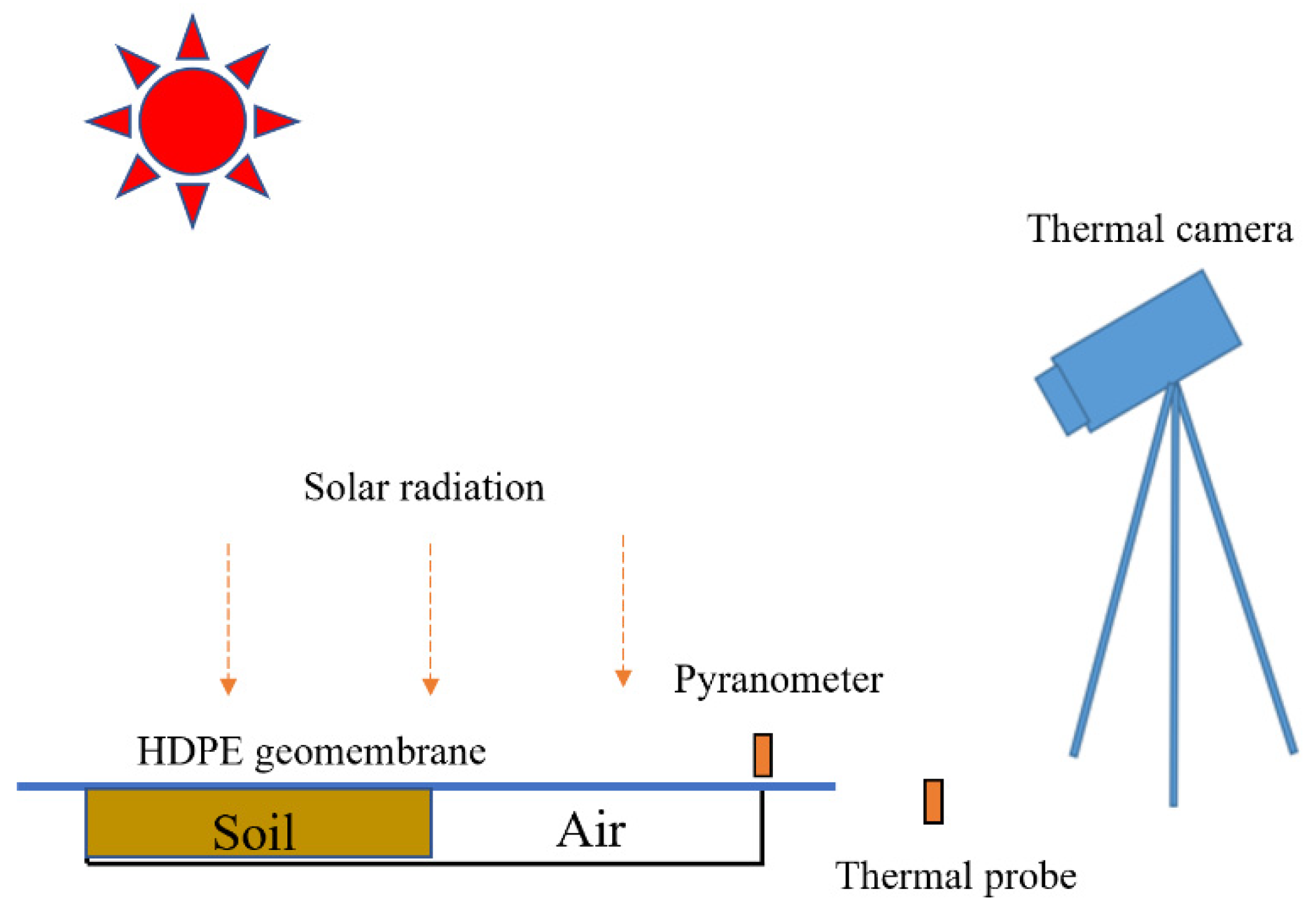
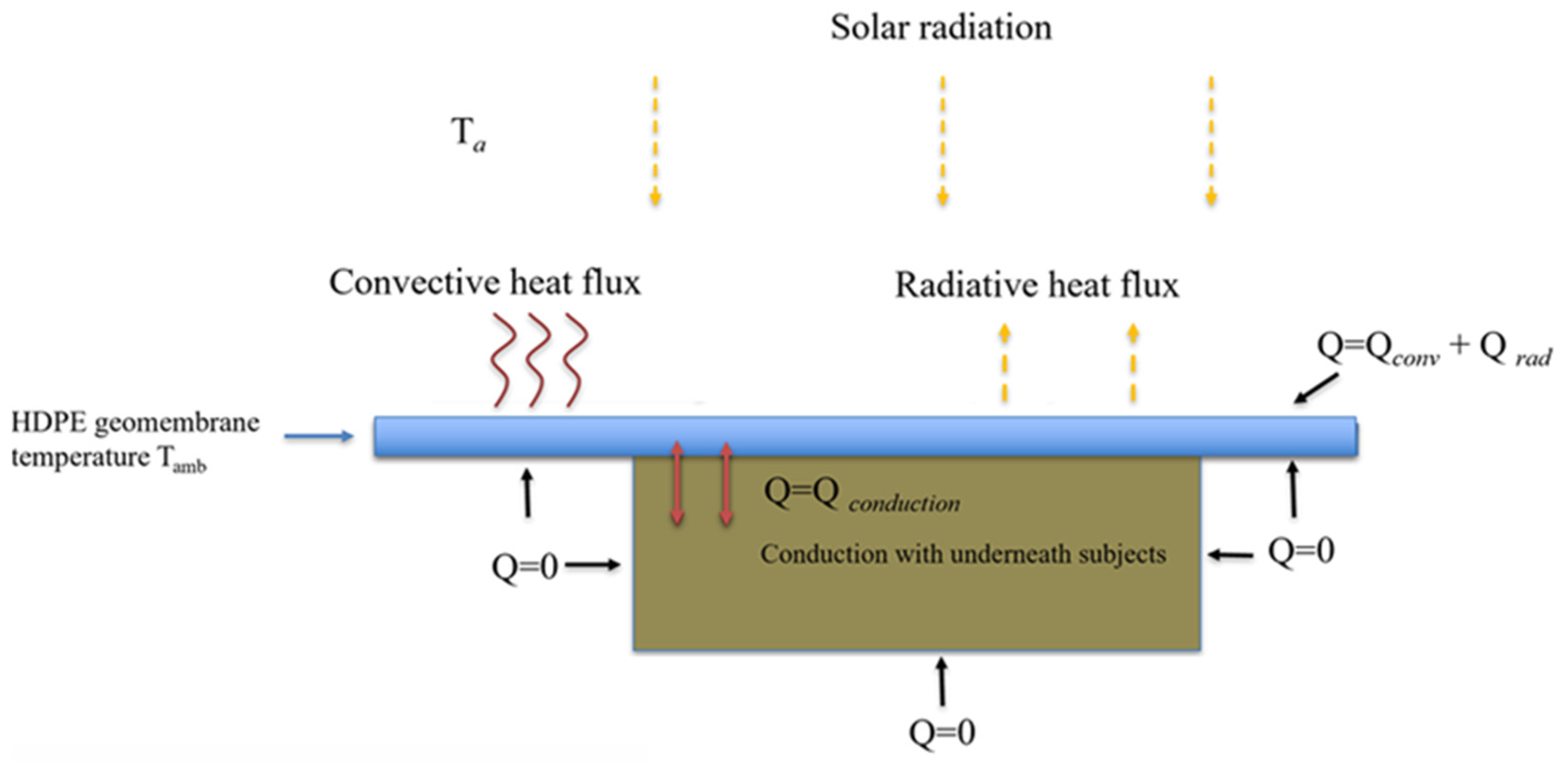
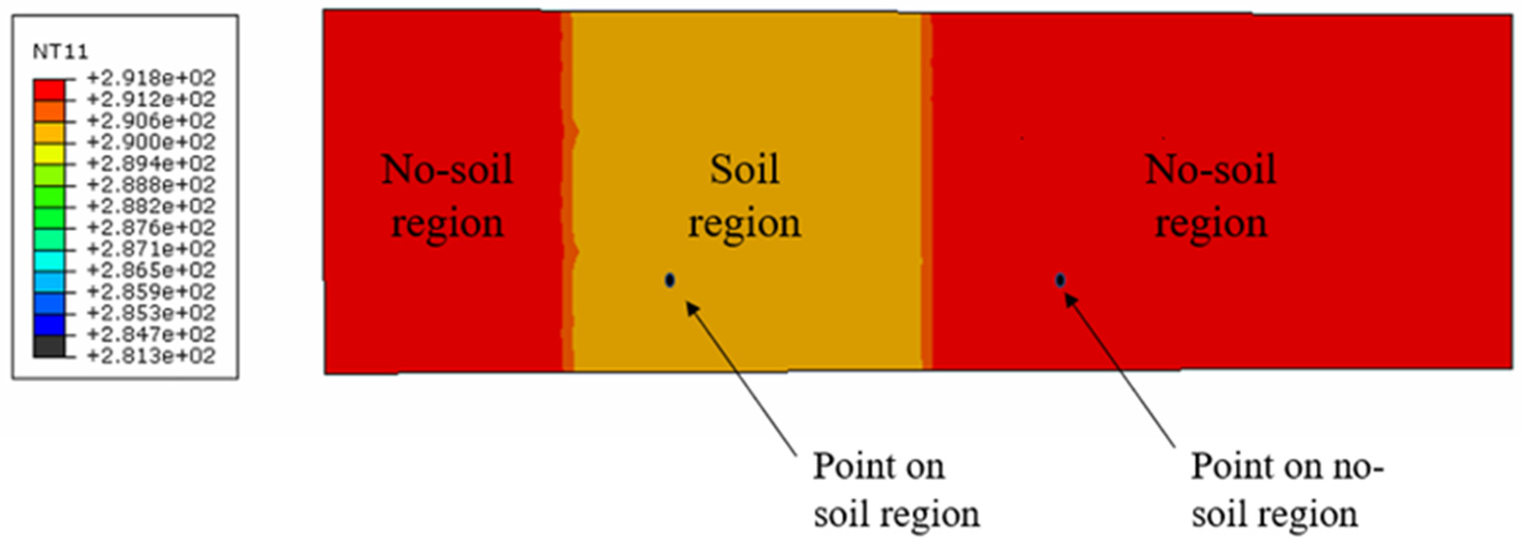
The relevant boundary conditions for the model are indicated in more detail in Figure 5, in a cross-sectional view. The intensity of the incident solar radiation is denoted by $I\left(t\right)$. Heat transfer from the top surface of the geomembrane occurs by convection and radiation [25,26]:

$$Q=Q_{conv}+Q_{rad}$$

(1)

The convective heat flux $Q\mathit{conv}$ is characterised by Newton’s law

$$Q_{conv}=h_c\left[T\left(t\right)-T_a\left(t\right)\right],$$

(2)

where $T\mathrm{and} T_a$ denote, respectively, the membrane temperature and ambient temperature at a time instant t and $h_c$ denotes the convective heat transfer coefficient. Radiative heat transfer for the HDPE membrane satisfied the Stefan–Boltzmann law, adapted for grey-body radiation [25,26]. Allowing for a radiative heat flux from the surroundings, the net radiative heat flux at the surface of a geomembrane can be written as follows:

$$Q_{rad}=\epsilon \sigma \left(T^4-T_a^4\right)$$

(3)

where $T \mathrm{and} T_a$ must now be interpreted as absolute temperatures, $\sigma$ denotes the Stefan–Boltzmann constant and $\epsilon$ the emissivity, which is equal to the absorptivity $\alpha$ according to Kirchoff’s law. For the range of temperatures encountered in this context, the difference $T-T_a$ is relatively small compared with the absolute ambient temperature $T_a$, so Equation (3) can be rewritten in the form

$$\begin{gathered} Q_{rad}=h_r\left[T\left(t\right)-T_a\left(t\right)\right] \\ {h}_r\approx 4\epsilon \sigma T_a^3 \end{gathered}$$

(4)

Accordingly, Equation (1) can now be rewritten as

$$\begin{gathered} Q=h\left[T\left(t\right)-T_a\left(t\right)\right] \\ h=h_c+h_r \end{gathered}$$

(5)

According to the experimental measurements of Pelte et al. [27], a representative value for the combined heat transfer coefficient for a horizontal geomembrane is $h=13 {\mathrm{Wm}}^{-2}{\mathrm{K}}^{-1}$, and this value was used in the FE model. The other relevant thermal properties for the model are summarised in

Table 5. Summary of material properties in the experiment.

Material	Density (kg/m3)	Thermal Conductivity (W/m*K)	Specific Heat (J/kg*K)	Thermal Diffusivity (mm2/s)
HDPE geomembrane	940 [35]	0.44 [35]	1900 [35]	0.246
Air (at 20 °C)	1.2754	0.138	1000	19
Water (at 20 °C)	997	0.6	4184	0.144
Soil	1350 [28]	0.47 [31]	1900 [32]	0.183
Scum	913 [29]	0.5 [30]	1400 [33]	0.391

.

For simplicity, it is assumed that there is no heat flux across the external boundaries of the model on the underside of the membrane, i.e., $Q=0,$ as shown in Figure 5. However, the membrane is assumed to be in perfect thermal contact with the soil substrate in the soil region, i.e., both temperature and heat flux are continuous across that interface.

The next step in characterising the cooling kinetics is to estimate the Biot number

$$\mathit{Bi}=\frac{h{L}_c}{k}$$

(6)

where k denotes the thermal conductivity and $L_c$ denotes an appropriate characteristic length, which in this case can be assumed to be the membrane thickness. This leads to $\mathit{Bi}\approx 0.06$. As this value is less than 0.1, the temperature gradient across the membrane thickness can be ignored [25,26]. Accordingly, the heat balance for a geomembrane on air (or biogas) can be written as follows:

$$\rho CL\frac{dT\left(t\right)}{dt}=h\left[T\left(t\right)-T_a\left(t\right)\right]$$

(7)

where $\rho ,C,\mathrm{and} L$ denote, respectively, the membrane’s density, specific heat and thickness. Assuming for simplicity that the ambient temperature can be regarded as being constant, or only slowly time varying, Equation (7) can be integrated to obtain

$$\begin{gathered} T\left(t\right)=T_a+\left(T_i-T_a\right)e^{-bt}, \\ \tau =b^{-1}=\frac{\rho CL}{h} \end{gathered}$$

(8)

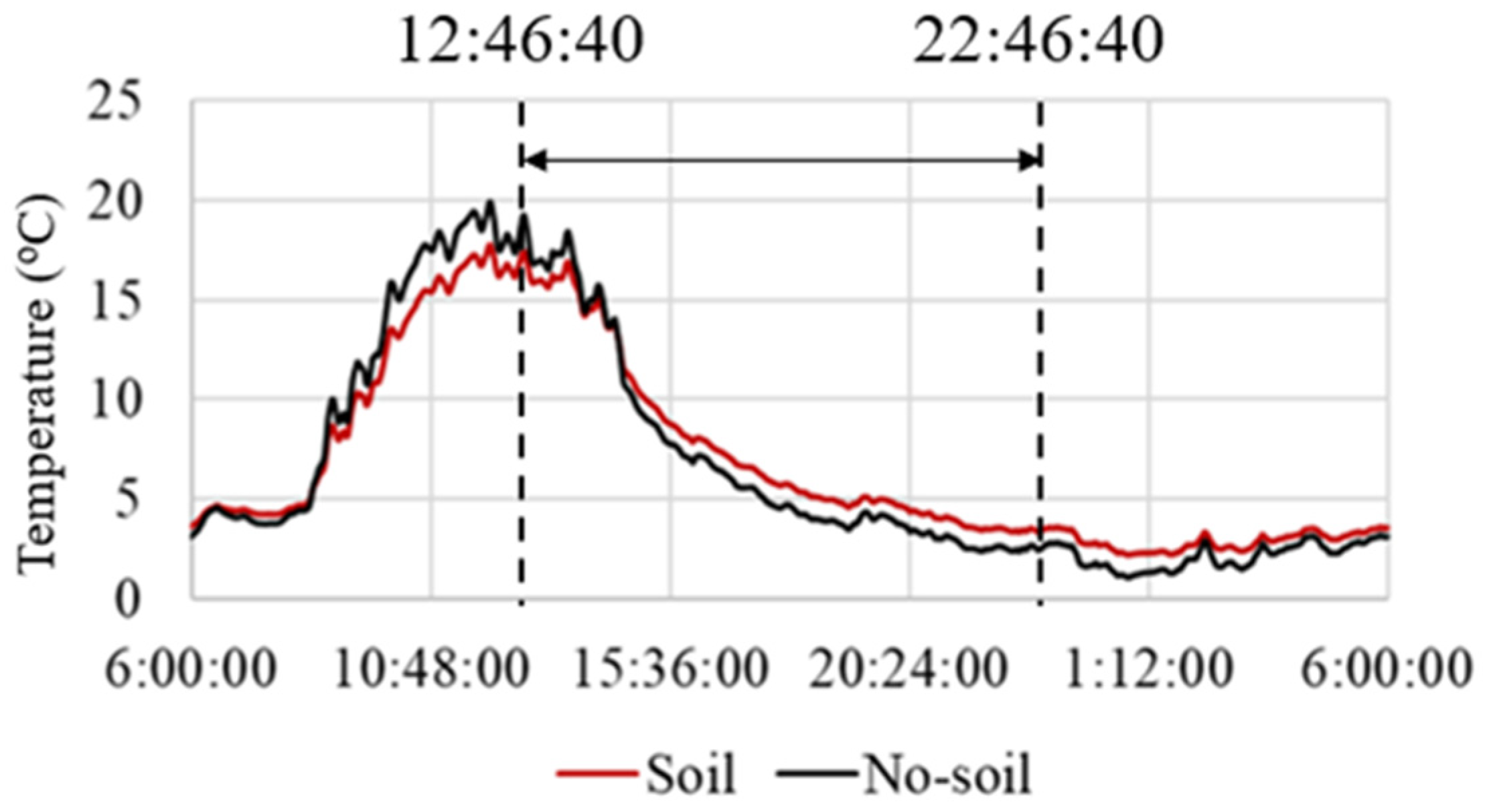
where $T_i$ denotes the initial temperature and b the cooling constant. The exponential decay law in Equation (8) applies strictly only for the geomembrane in contact with air or biogas. However, as shown in our previous work [9,10,11], it is also possible to allocate a value of the cooling constant for regions where the geomembrane is in contact with soil (simulating scum) by fitting the (measured or calculated) thermal transients to an exponential decay law.

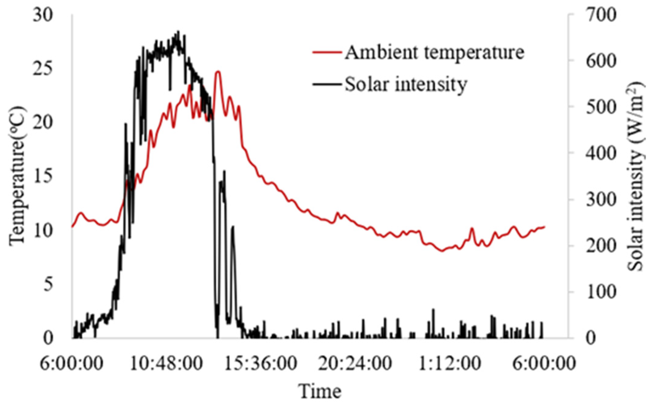
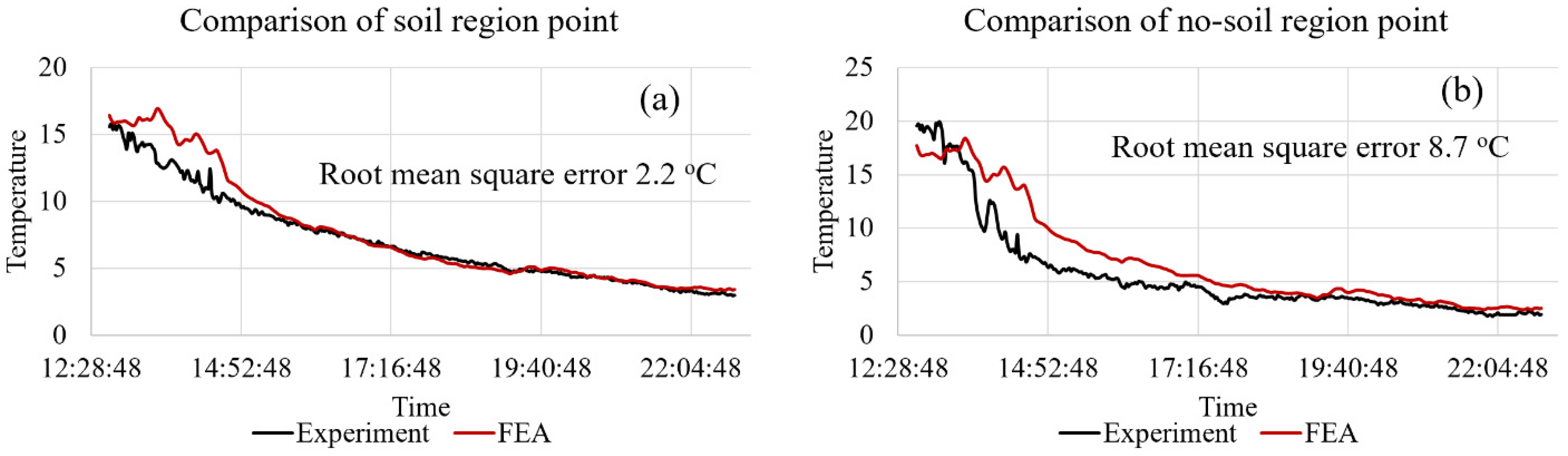
The FE model was used to analyse the temperature change on the HDPE geomembrane, using the measured solar intensity and ambient temperature as inputs. The geometry of the FE model is shown in Figure 4 with a mesh size of 1 mm.

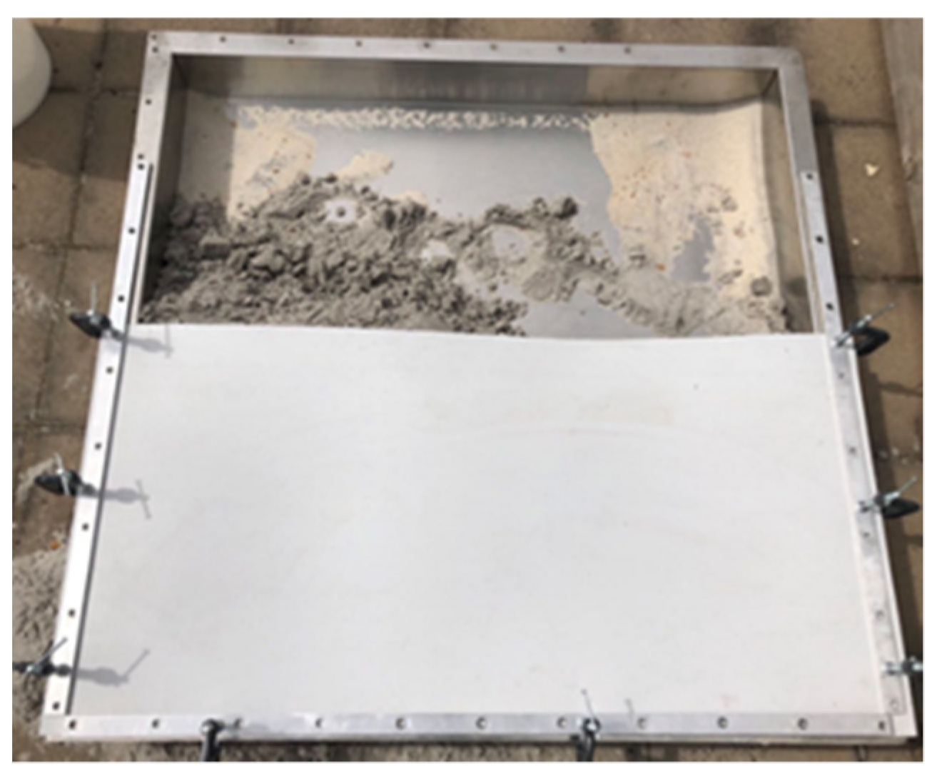
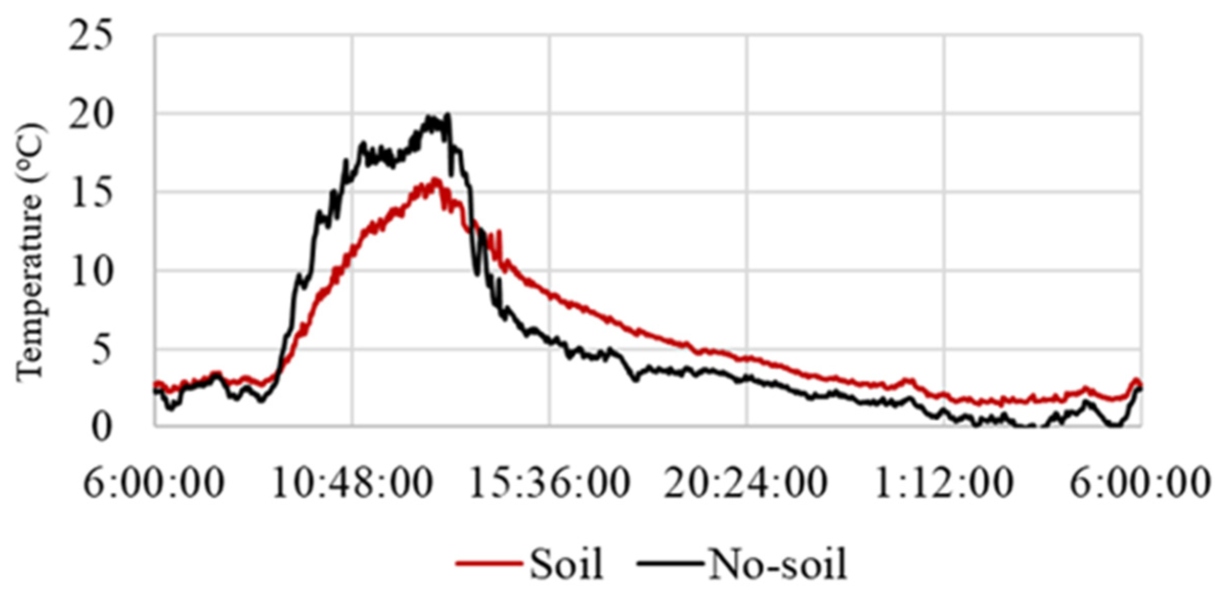
The experiments described in Section 2.1 used clayey soil since it is reported that clayey soil has similar density [28,29], thermal conductivity [30,31] and specific heat [32,33] as scumbergs. The thermal properties of each material are summarised in Table 5. The emissivity of the HDPE geomembrane at the WTP is approximately 0.9 [9,10,11]. The thermal expansion effect of the HDPE geomembrane was neglected in this study because it does not affect the thermal transient response. The time-dependent thermal FE analysis was conducted over a 24 h period with a time step of 100 s.

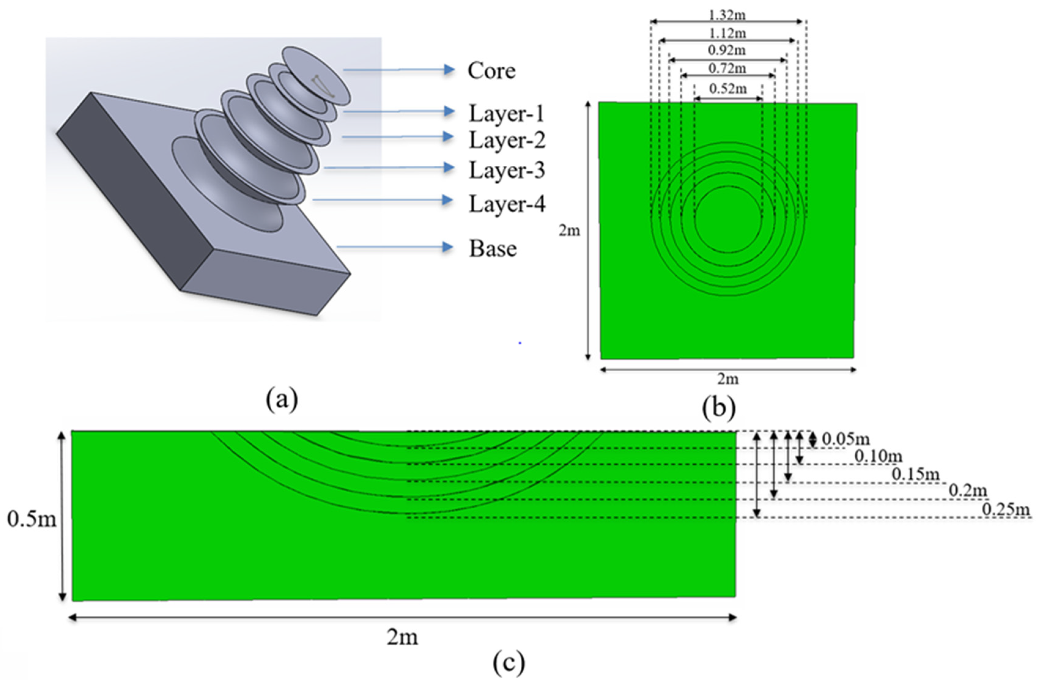
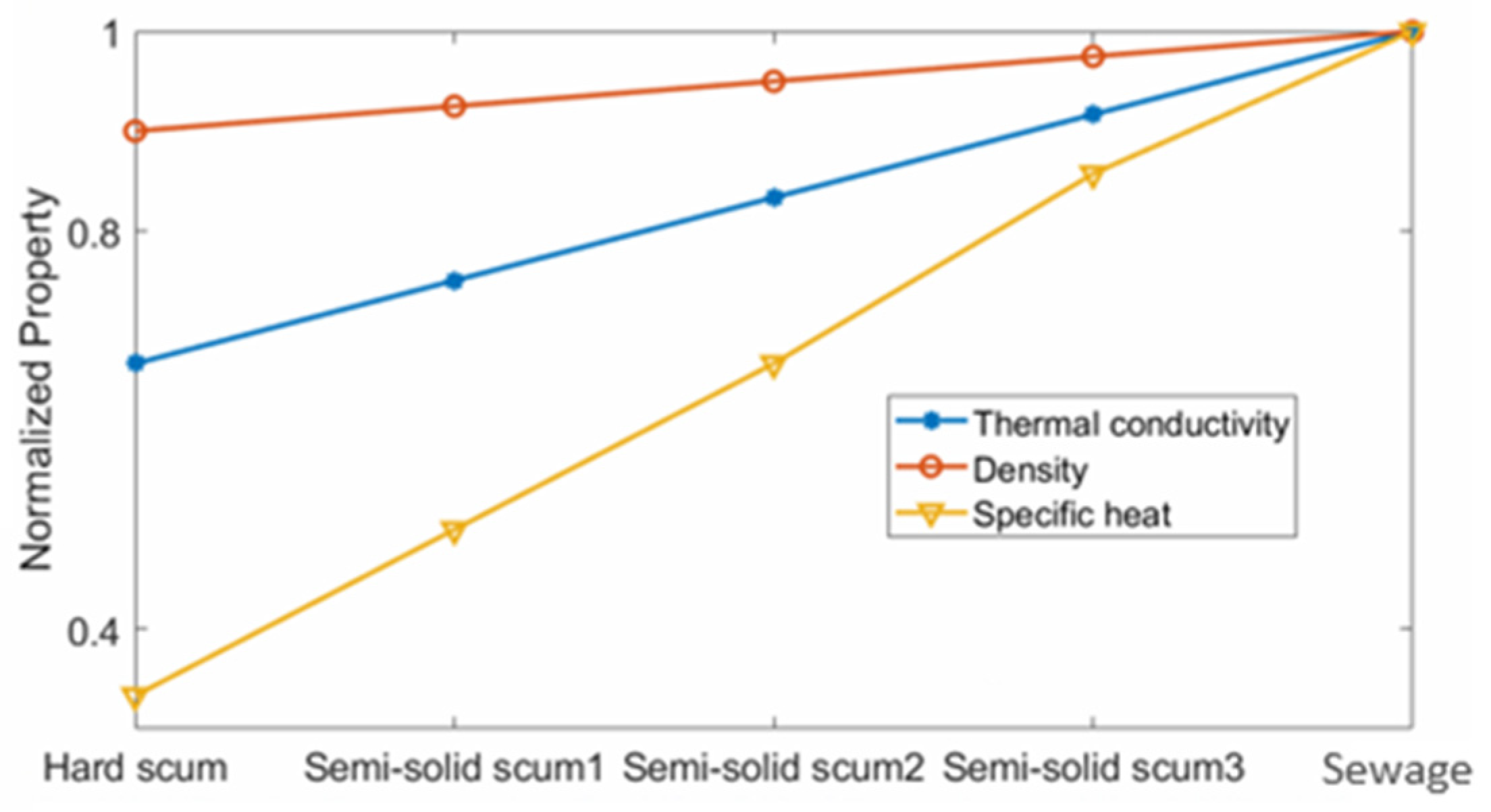
To simulate the effect of scum accumulation, the FE model of the soil substrate region in Figure 4 was modified, as shown in Figure 6. The substrate was partitioned into six regions, as indicated schematically in Figure 6a, and in plan view and cross-sectional view in Figure 6b,c, respectively. The thermal properties changed stepwise across those regions, from those appropriate for liquid sewage, which was simulated as water, to those of hard scum (cf. Table 5), through 3 intermediate values obtained by linear interpolation, as indicated in Figure 7. The extreme values are based on those reported in [33,34], and their applicability for the WTP will be further discussed below.

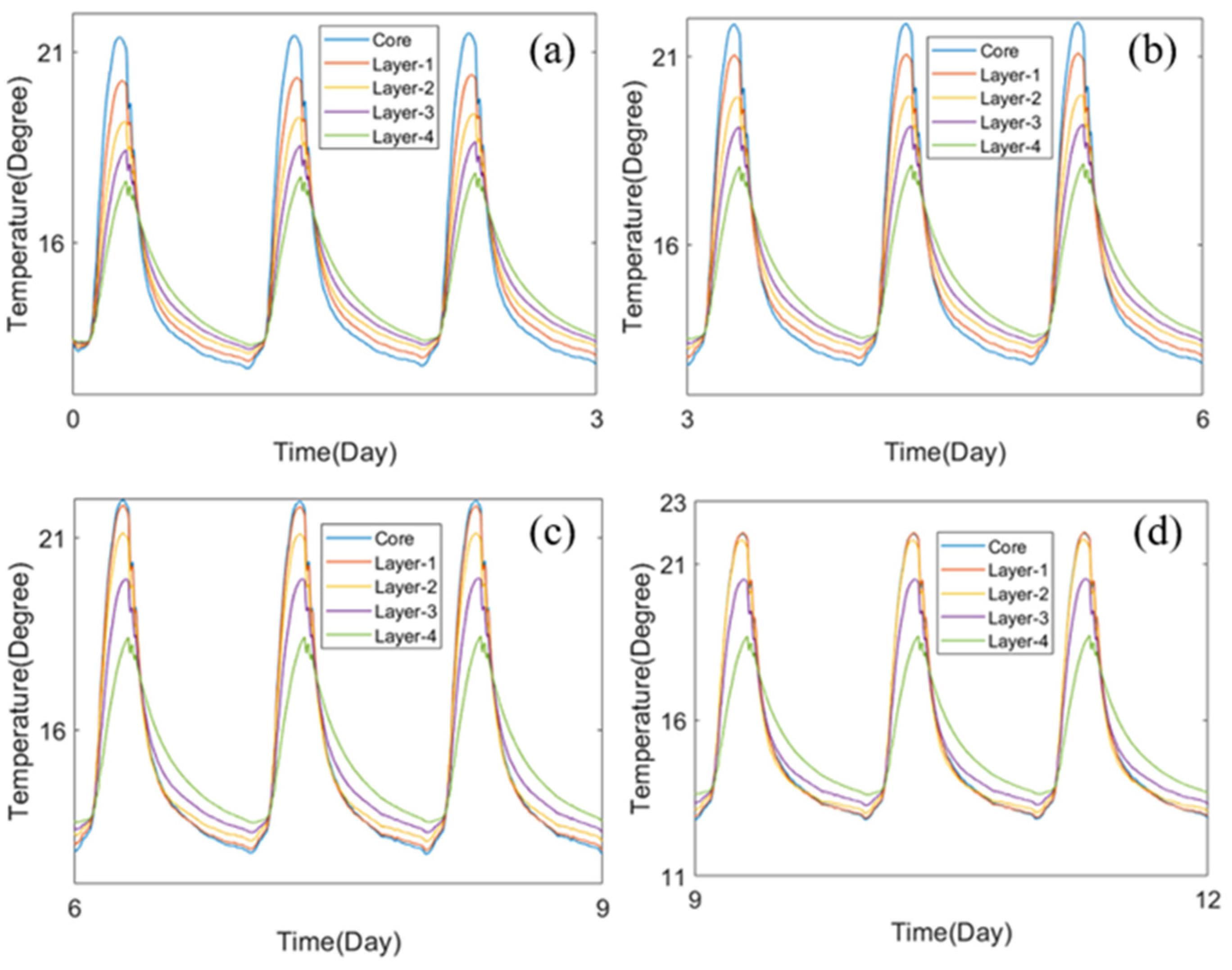
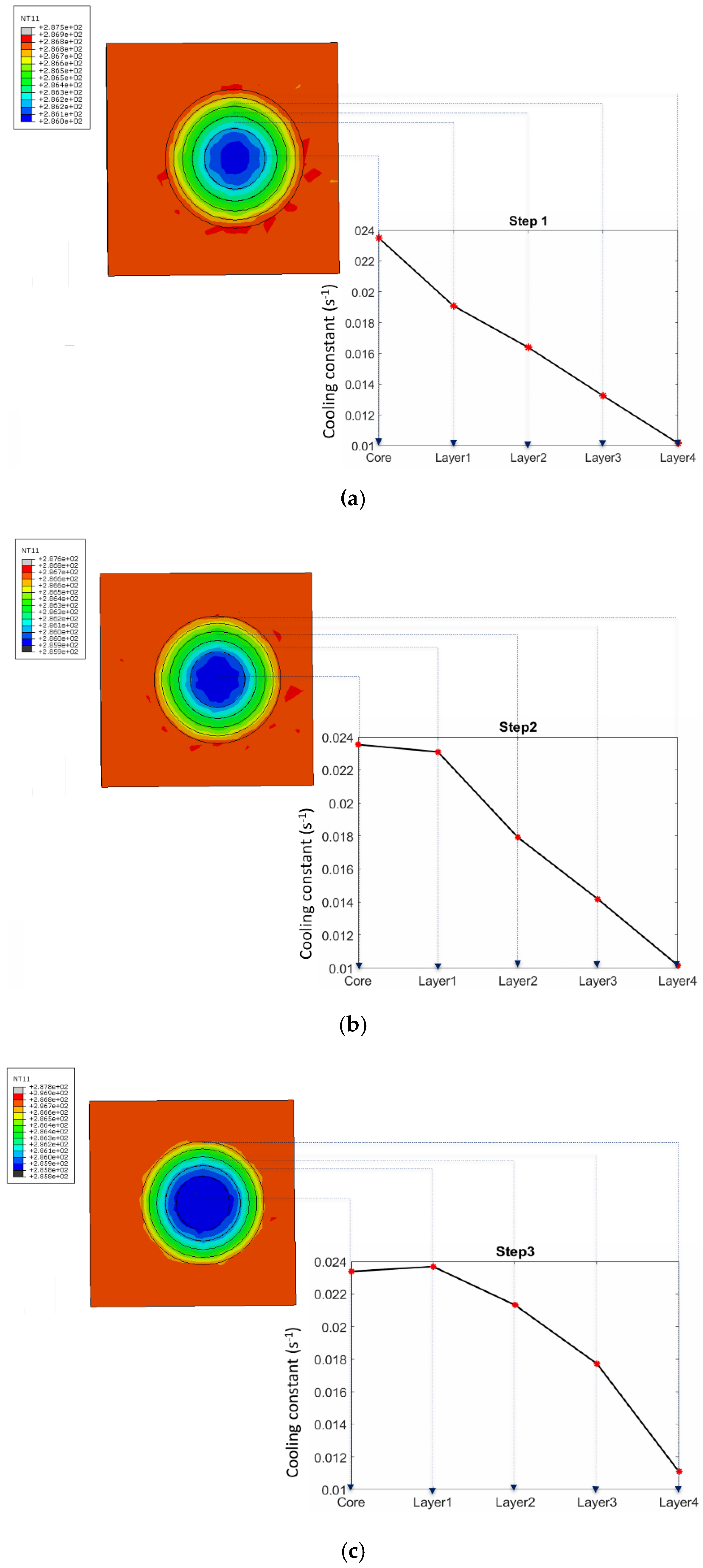
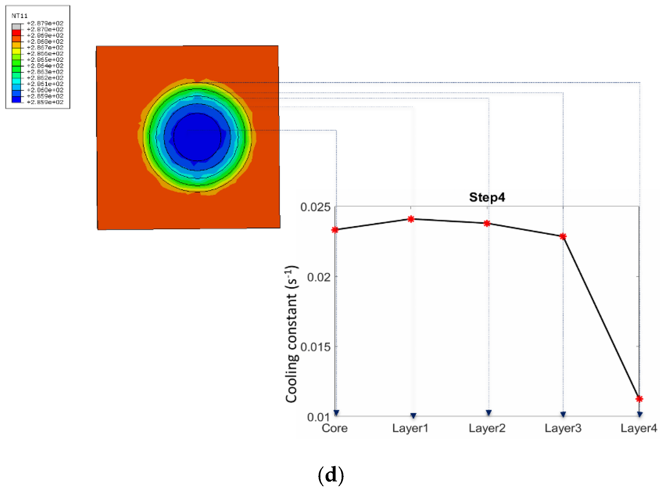
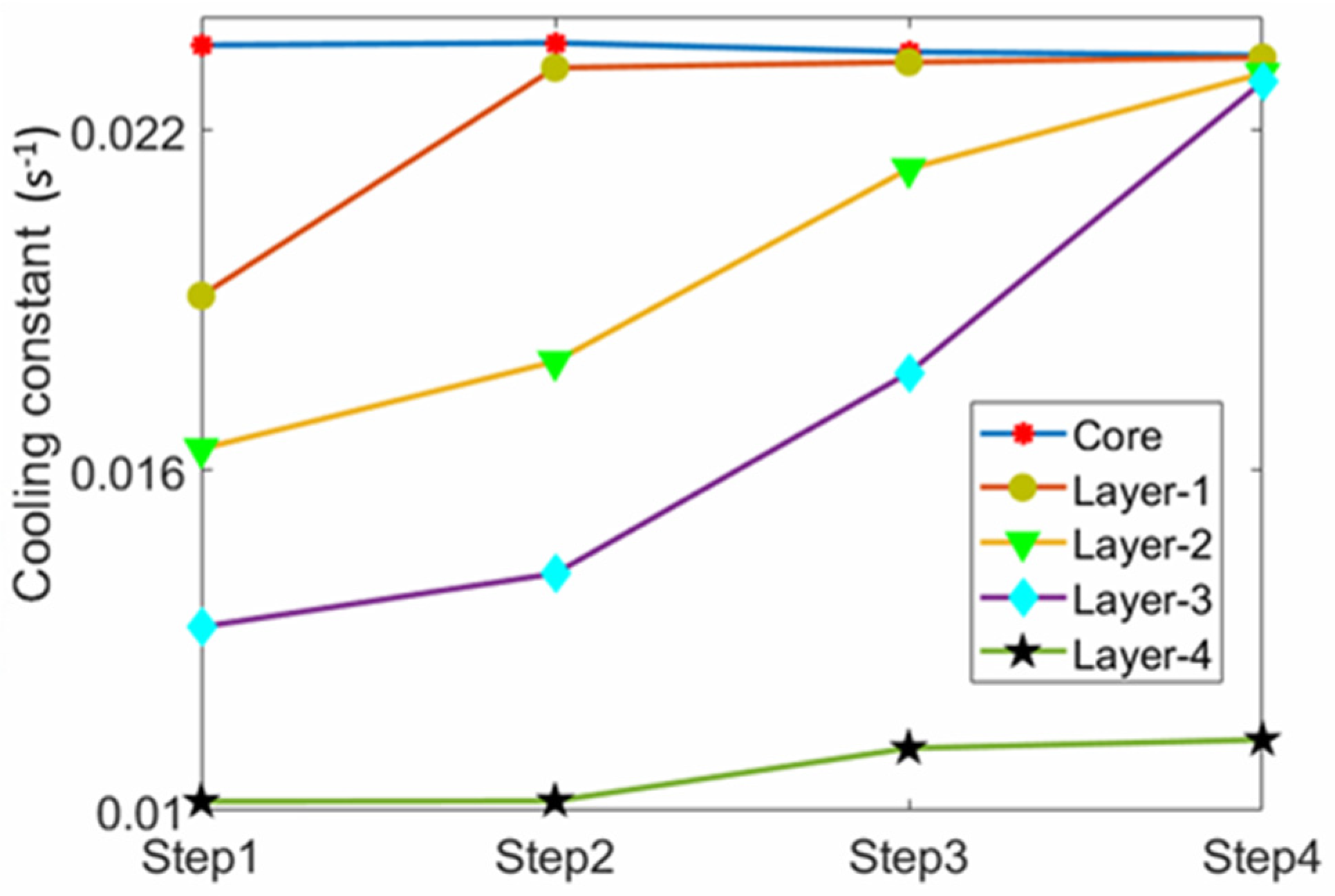
The progressive accumulation of scum was simulated through a stepwise change in properties over time. The model was subjected to 12 cycles of the same 24 h variation in solar intensity and ambient temperature described above. These 12 cycles were grouped into four sets lasting 3 days each. The thermal properties were varied stepwise over 4 time steps corresponding to these four sets, as summarised in

Table 6. Instances state in each analysis step.

Region	Step 1	Step 2	Step 3	Step 4
Core	Hard scum	Hard scum	Hard scum	Hard scum
Layer 1	Semi-solid scum 1	Hard scum	Hard scum	Hard scum
Layer 2	Semi-solid scum 2	Semi-solid scum 1	Hard scum	Hard scum
Layer 3	Semi-solid scum 3	Semi-solid scum 2	Semi-solid scum 1	Hard scum
Layer 4	Sewage	Semi-solid scum 3	Semi-solid scum 2	Semi-solid scum 1
Base	Sewage	Sewage	Sewage	Sewage

. During each step, the temperature profile on the membrane surface was monitored at five locations corresponding to the five regions identified in Figure 6, viz. core, and layer 1 through layer 4. The geomembrane thickness and boundary conditions were the same as in Section 2.

3. Results and Discussions

3.1. Using the Cooling Constant to Identify the Presence of Simulated Scumberg under the Geomembrane

Figure 8 shows the experimental records of the solar intensity and ambient temperature over a 24 h period, while Figure 9 shows the corresponding temperature profiles recorded at a point on the surface of the geomembrane that is in contact with the garden soil and a point within the no-soil region. The pyranometer was set up to measure solar intensity with a sampling rate of 3 Hz, while the temperature probe was set to measure the ambient temperature once every 10 min. It can be observed that the solar intensity increased from 0 W/m² at 6 AM up to ~650 W/m² at around noon and decreased thereafter due to extensive cloud cover. After sunset, the solar intensity remained close to 0 W/m² until sunrise the following morning.

The experimental data in Figure 8 was used as input into the FE model for predicting the surface temperature of the HDPE geomembrane for comparison with the experimentally recorded temperature.

Using the results shown in Figure 9, the initial temperature across the surface of the membrane was set at 3 °C to correspond to experimental data. Temperatures of both regions increased due to the incident solar radiation. The maximum temperature was attained at around 11:30:00; the HDPE geomembrane cooled in the afternoon with the reduction in solar radiation and ambient temperature. Figure 10 shows the surface temperature distribution predicted by the FE model at 11:37:00. The thermal contrast at this time spot clearly differentiated the soil region from the no-soil region. Figure 11 shows the computed temperature profiles at a point within the soil region and a point within the no-soil region. It can be seen that the FE analysis (FEA) correctly captured the experimentally observed temperature profile shown in Figure 9.

A more detailed comparison between measurement and simulation is shown in Figure 12 for the time interval from 12:46:40 to 22:46:40. It can be seen that the temperature profiles were correctly captured. The root-mean-square error was approximately 2.2 °C within the no-soil region and 8.7 °C within the soil region.

Table 7. Illustration of curve-fitted cooling constants.

	Experiment		FEA
	Soil region	No-soil region	Soil region	No-soil region
Cooling constant(s−1)	0.0077	0.0162	0.0067	0.0123
R-squared value of curve fitting	0.99	0.95	0.97	0.95

shows the values of the cooling constants obtained by fitting an exponential decay curve, given by Equation (8), to the cooling transients shown in Figure 12. It can be seen that there was reasonable agreement between the experimental and FEA values. In particular, the FEA correctly predicted a doubling of the cooling constant (corresponding to the halving of the decay time) for a point within the no-soil region relative to one within the soil region. This agreement provides confidence in the predictive capability of the FE model.

3.2. Monitoring Scum Accumulation

As described in Section 2 above, the progressive accumulation of scum was simulated through a stepwise change in properties over time. The model was subjected to 12 cycles of the same 24 h variation in solar intensity and ambient temperature that was used earlier in Section 2. These 12 cycles were grouped into four sets lasting 3 days each. The thermal properties were varied stepwise over 4 time steps corresponding to these four sets, as summarised in Table 6. A typical set of results is shown in Figure 13. As shown in Figure 13a, in the first 3 days (step 1), due to the different heat transfer material properties, each region described in Table 6 reached different maximum temperatures during the heating cycle (i.e., during the day). During nightfall, these regions cooled to the minimum temperature resulting from the reduced solar intensity and ambient temperature. It was observed that the core region had the highest cooling rate compared with the others. As each region was transformed to hard scum (see Table 6) over the simulated 12-day simulation, the corresponding surface temperatures are shown in Figure 13b–d.

To further understand the scum transition process, these temperature profiles of each step were then used to calculate cooling constants by fitting the profiles to the Newton’s law of cooling, as explained earlier in Section 2. The resulting values of the cooling constant within the five regions are shown in Figure 14a–d for each of the four time steps. These results show the temperature contour at each time step. The temperature decay profiles of each node at the different regions of the geomembrane were extracted to calculate the cooling constant. The change in the cooling constant with time is summarised in Figure 15. It can be seen that there was a clear change in the value of the cooling constant corresponding to the progressive change of the state of the scum. It seems reasonable to expect that this change could provide the basis for a practical, real-world quantitative characterisation of the state of scum accumulation beneath the floating covers at the WTP.

4. Discussions

A thermographic approach to identify and monitor the development of scum accumulation under the geomembrane cover is presented in this paper. The physical size of the cover (450 m × 170 m) and the hazardous operating environment demand an area assessment technique that is non-contact and can be operated at a safe distance from the cover. The ability to conduct these assessments remotely from the cover will also remove the need for a person to conduct the current practice of “walk-the-cover” inspection that delivers only a qualitative assessment of the state and extent of the scum based on the to-the-foot feel during these inspections. Therefore, this thermographic approach will enhance the safe working condition at the WTP. Due to the size of the cover, there is currently no practical and efficient technique available for this large-area assessment. As a result, the research team is currently working on integrating our UAV-enabled photogrammetry assessment with machine learning capability to assess the extent and to infer the state of the scum accumulated beneath the cover [19,21]. The work presented in this paper shows the potential of the thermographic technique as a tool to quantify the extent and state of the scum beneath the cover. This thermographic technique along with the work described in [19,21] will aim to enhance the current practice at the WTP. It is recognised that the results summarized in Figure 15 are dependent on the assumed geometry and time evolution of substrate material properties, which may not be fully representative of the actual process of scum accumulation at the WTP. Field trials of the proposed approach are currently being planned, which may provide more reliable geometry and material properties for future modelling. However, it seems reasonable to expect that the change in the cooling constant that is predicted by the current modelling assumptions is representative of what would be measured in practice and, therefore, that monitoring the cooling constant should constitute a promising approach for a quantitative characterisation of scum accumulation beneath the floating covers at the WTP.

5. Conclusions

This paper introduces a proactive non-contact temperature-monitoring technique for the floating HDPE geomembrane covers at the anaerobic sewage treatment lagoons operated by the MWC at the WTP. The proposed technique relies on naturally occurring variations in solar intensity to cause thermal transients in the surface temperature of the geomembrane. A laboratory-scale experimental measurement of the surface temperature profile, using a clayey garden-type soil to simulate scum, was used as a basis for assessing the predictive accuracy of an FE model that used the experimentally recorded solar intensity and ambient temperature as inputs. This assessment confirmed the adequacy of the FE model for predicting in particular the cooling constants obtained by fitting an exponential decay law to the thermal transients.

The FE model was then modified to simulate the effect of a progressive accumulation of scum beneath the HDPE cover. The results indicate a detectable change in the cooling constant with time at different locations of the cover material, reflecting different simulated states of scum accumulation beneath the cover. These results suggest that an in situ measurement of the cooling constant could potentially provide a more quantitative assessment of scum accumulation than is available from current inspection practice. This in turn could be used for a more efficient scheduling of maintenance actions, as well as informing longer-term decisions regarding repair or replacement options for the cover. Field trials of the proposed approach are currently being planned, which may provide more reliable geometry and material properties for future modelling. This non-contact technique of monitoring the cooling constant should constitute a promising approach for a quantitative characterisation of scum accumulation beneath the floating covers at the WTP.

References

1. Rowe, R.K.; Islam, M.Z.; Brachman, R.W.I.; Arnepalli, D.N.; Ewais, A.R. Antioxidant Depletion from a High Density Polyethylene Geomembrane under Simulated Landfill Conditions. J. Geotech. Geoenvironmental Eng. 2010, 136, 930–939. [Google Scholar] [CrossRef]
2. Sangam, H.P. Performance of HDPE Geomembrane Liners in Landfill Applications; ProQuest Dissertations Publishing: Ann Arbor, MI, USA, 2001. [Google Scholar]
3. Ng, H.B. HDPE Lined Water Reservoirs for Power Generating Stations. In Geosynthetics in Civil and Environmental Engineering; Springer: Berlin/Heidelberg, Germany, 2009; pp. 769–774. [Google Scholar] [CrossRef]
4. Fourie, A.; Bouazza, A.; Lupo, J.; Abrao, P. Improving the performance of mining infrastructure through the judicious use of geosynthetics. In Proceedings of the 9th International Conference on Geosynthetics: Geosynthetics for a Changing World, Guaruja, Brazil, 23–27 May 2010; Palmeira, E.M., Vidal, D.M., Sayao, A.S.J.F., Ehrlich, M., Eds.; International Geosynthetics Society Brazil: Guaruja, Brazil, 2010; pp. 193–218. [Google Scholar]
5. Rowe, R.; Rimal, S.; Sangam, H. Ageing of HDPE geomembrane exposed to air, water and leachate at different temperatures☆. Geotext. Geomembr. 2008, 27, 137–151. [Google Scholar] [CrossRef]
6. Sewage treatment process at Western Treatment Plant. 2020. Available online: https://www.melbournewater.com.au/ (accessed on 26 November 2021).
7. VEEA. 2014. Available online: https://issuu.com/veea14/docs/8292_engineers_aust_2014_veea_onlin (accessed on 26 November 2021).
8. AWA. Available online: http://www.awa.asn.au/AWA_MBRR/About_AWA/Awards/State_Awards/VIC_Winners.aspx (accessed on 26 November 2021).
9. Ma, Y.; Wong, L.; Vien, B.; Kuen, T.; Rajic, N.; Kodikara, J.; Chiu, W. Quasi-Active Thermal Imaging of Large Floating Covers Using Ambient Solar Energy. Remote Sens. 2020, 12, 3455. [Google Scholar] [CrossRef]
10. Ma, Y.; Rose, F.; Wong, L.; Vien, B.; Kuen, T.; Rajic, N.; Kodikara, J.; Chiu, W. Detection of Defects in Geomembranes Using Quasi-Active Infrared Thermography. Sensors 2021, 21, 5365. [Google Scholar] [CrossRef]
11. Ma, Y.; Wong, L.; Vien, B.S.; Kuen, T.; Rajic, N.; Rose, L.R.F.; Kodikara, J.; Chiu, W.K. Quasi-Active Thermography for Structural Health Assessment of Large Geomembranes. Mater. Res. Proc. 2021, 18, 79–86. [Google Scholar]
12. Omar, T.; Nehdi, M.L. Remote sensing of concrete bridge decks using unmanned aerial vehicle infrared thermography. Autom. Constr. 2017, 83, 360–371. [Google Scholar] [CrossRef]
13. Omar, T.; Nehdi, M.L.; Zayed, T. Infrared thermography model for automated detection of delamination in RC bridge decks. Constr. Build. Mater. 2018, 168, 313–327. [Google Scholar] [CrossRef]
14. Brooke, C. Thermal Imaging for the Archaeological Investigation of Historic Buildings. Remote Sens. 2018, 10, 1401. [Google Scholar] [CrossRef] [Green Version]
15. Ostańska, A. Thermal Imaging for Detection of Defects in Envelopes of Buildings in Use: Qualitative and Quantitative Analysis of Building Energy Performance. Period. Polytech. Civ. Eng. 2018, 62, 939. [Google Scholar] [CrossRef]
16. Bhalla, S.; Tuli, S.; Arora, R. Defect detection in concrete structures using thermal imaging techniques. Exp. Tech. 2010, 35, 39–43. [Google Scholar] [CrossRef]
17. Avdelidis, N.; Almond, D. Transient thermography as a through skin imaging technique for aircraft assembly: Modelling and experimental results. Infrared Phys. Technol. 2004, 45, 103–114. [Google Scholar] [CrossRef]
18. Han, X.; Favro, L.D.; Thomas, R.L. Thermal Wave Imaging for Characterizing Structures in Aging Aircraft. MRS Proc. 1997, 503. [Google Scholar] [CrossRef]
19. Wong, L.; Vien, B.S.; Ma, Y.; Kuen, T.; Courtney, F.; Kodikara, J.; Rose, F.; Chiu, W.K. Development of Scum Geometrical Monitoring Beneath Floating Covers Aided by UAV Photogrammetry. Mater. Res. Proc. 2021, 18, 71–78. [Google Scholar] [CrossRef]
20. Vien, B.S.; Wong, L.; Kuen, T.; Courtney, F.; Kodikara, J.; Chiu, W.K. Strain Monitoring Strategy of Deformed Membrane Cover using Unmanned Aerial Vehicle-Assisted 3D Photogrammetry. Remote Sens. 2020, 12, 2738. [Google Scholar] [CrossRef]
21. Wong, L.; Vien, B.S.; Ma, Y.; Kuen, T.; Courtney, F.; Kodikara, J.; Chiu, W.K. Remote Monitoring of Floating Covers Using UAV Photogrammetry. Remote Sens. 2020, 12, 1118. [Google Scholar] [CrossRef] [Green Version]
22. Apogee. Apogee Instruments Owner’s Manual Pyranometer Models SP-110 and SP-230; Apogee: Logan, UT, USA, 2020. [Google Scholar]
23. FLIR. User’s Manual FLIR A6xx Series; FLIR Systems: Wilsonville, OR, USA, 2016. [Google Scholar]
24. Abaqus Analysis User’s Guide (6.14). Abaqus Analysis User’s Guide. 2021. Available online: http://130.149.89.49:2080/v6.14/books/usb/default.html (accessed on 26 November 2021).
25. Bergman, T.L.; Lavine, A.; Incropera, F.P.; ProQuest. Fundamentals of Heat and Mass Transfer, 8th ed.; Wiley: Hoboken, NJ, USA, 2017. [Google Scholar]
26. Cengel, Y.A.; Ghajar, A.J. Heat and Mass Transfer: Fundamentals & Applications, 4th ed.; McGraw Hill Higher Education: New York, NY, USA, 2021. [Google Scholar]
27. Pelte, T.; Pierson, P.; Gourc, J. Thermal Analysis of Geomembrane Exposed to Solar Radiation. Geosynth. Int. 1994, 1, 21–44. [Google Scholar] [CrossRef]
28. Zeri, M.; Alvalá, R.C.S.; Carneiro, R.; Cunha-Zeri, G.; Costa, J.M.; Spatafora, L.R.; Urbano, D.; Vall-Llossera, M.; Marengo, J. Tools for Communicating Agricultural Drought over the Brazilian Semiarid Using the Soil Moisture Index. Water 2018, 10, 1421. [Google Scholar] [CrossRef] [Green Version]
29. Balasubramanian, R.; Sircar, A.; Sivakumar, P.; Ashokkumar, V. Conversion of bio-solids (scum) from tannery effluent treatment plant into biodiesel. Energy Sources Part A Recovery Util. Environ. Eff. 2018, 40, 959–967. [Google Scholar] [CrossRef]
30. Song, H.W.; Park, K.J.; Han, S.K.; Jung, H.S. Thermal conductivity characteristics of dewatered sewage sludge by thermal hydrolysis reaction. J. Air Waste Manag. Assoc. 2014, 64, 1384–1389. [Google Scholar] [CrossRef] [Green Version]
31. Nikiforova, T.; Savytskyi, M.; Limam, K.; Bosschaerts, W.; Belarbi, R. Methods and Results of Experimental Researches of Thermal Conductivity of Soils. Energy Procedia 2013, 42, 775–783. [Google Scholar] [CrossRef] [Green Version]
32. Kodešová, R.; Vlasáková, M.; Fér, M.; Teplá, D.; Jakšík, O.; Neuberger, P.; Adamovský, R. Thermal properties of representative soils of the Czech Republic. Soil Water Res. 2013, 8, 141–150. [Google Scholar] [CrossRef] [Green Version]
33. Milhé, M.; Sauceau, M.; Arlabosse, P. Modeling of a continuous sewage sludge paddle dryer by coupling Markov chains with penetration theory. Appl. Math. Model. 2016, 40, 8201–8216. [Google Scholar] [CrossRef] [Green Version]
34. O’Kelly, B. Consolidation properties of a dewatered municipal sewage sludge. Can. Geotech. J. 2005, 42, 1350–1358. [Google Scholar] [CrossRef] [Green Version]
35. Thakare, A. Experimental investigation of possible use of hdpe as thermal storage material in thermal storage type solar cookers. Int. J. Res. Eng. Technol. 2015, 4, 92–99. [Google Scholar] [CrossRef]
Figure 1. Google Map view of one of the HDPE geomembrane floating covers on an anaerobic lagoon at the WTP in Werribee, Victoria, Australia.
Remotesensing 13 04857 g001
Figure 2. Test setup showing the HDPE geomembrane specimen, partly in contact with soil, simulating solid scum, and partly in contact with air (no-soil region), deployed across an aluminium tray.
Remotesensing 13 04857 g002
Figure 3. Illustration of the experimental setup showing the instrumentation.
Remotesensing 13 04857 g003
Figure 4. Illustration of the geometry of the FE model.
Remotesensing 13 04857 g004
Figure 5. Cross-sectional view of boundary conditions for heat transfer in the FE model.
Remotesensing 13 04857 g005
Figure 6. Illustration of geometry details of the substrates model. (a) Exploded view of the assembly. (b) Top view of the assembly. (c) Cross-sectional view of the assembly.
Remotesensing 13 04857 g006
Figure 7. Interpolated thermal properties of the base model. Thermal properties change from hard scum to sewage.
Remotesensing 13 04857 g007
Figure 8. The recorded solar intensity and ambient temperature profile.
Remotesensing 13 04857 g008
Figure 9. The experimental temperature profiles at points within the soil region and no-soil region on the HDPE geomembrane.
Remotesensing 13 04857 g009
Figure 10. Predicted temperature field across the geomembrane at 11:37:00 from the FE model.
Remotesensing 13 04857 g010
Figure 11. Predicted temperature profile of HDPE geomembrane from FE analysis.
Remotesensing 13 04857 g011
Figure 12. Comparison of FE results and experiment measurements for the surface temperature over (a) soil and (b) no-soil regions.
Remotesensing 13 04857 g012
Figure 13. Predicted temperature profiles for each region on the geomembrane. (a) temperature profiles of step 1. (b) temperature profiles of step 2. (c) temperature profiles of step 3. (d) temperature profiles of step 4.
Remotesensing 13 04857 g013
Figure 14. Illustration of cooling constant distributions of each layer over different steps in Table 6: (a) step 1, (b) step 2, (c) step 3 and (d) step 4.
Remotesensing 13 04857 g014aRemotesensing 13 04857 g014b
Figure 15. Illustration of cooling constant changes for each region on the geomembrane over the scum transition. Steps 1–4 described in Table 6.
Remotesensing 13 04857 g015