
Drone-Based Bathymetry Modeling for Mountainous Shallow Rivers in Taiwan Using Machine Learning


1
Department of Hydraulic and Ocean Engineering, National Cheng Kung University, Tainan City 70101, Taiwan
2
General Research Service Center, National Pingtung University of Science and Technology, Pingtung County 91201, Taiwan
3
Institute of Ocean Technology and Marine Affairs, National Cheng Kung University, Tainan City 70101, Taiwan
*
Author to whom correspondence should be addressed.
Remote Sens. 2022, 14(14), 3343; https://0-doi-org.brum.beds.ac.uk/10.3390/rs14143343
Submission received: 25 May 2022
/
Revised: 30 June 2022
/
Accepted: 6 July 2022
/
Published: 11 July 2022
(This article belongs to the Special Issue Remote Sensing in Water Engineering and Management)
Abstract
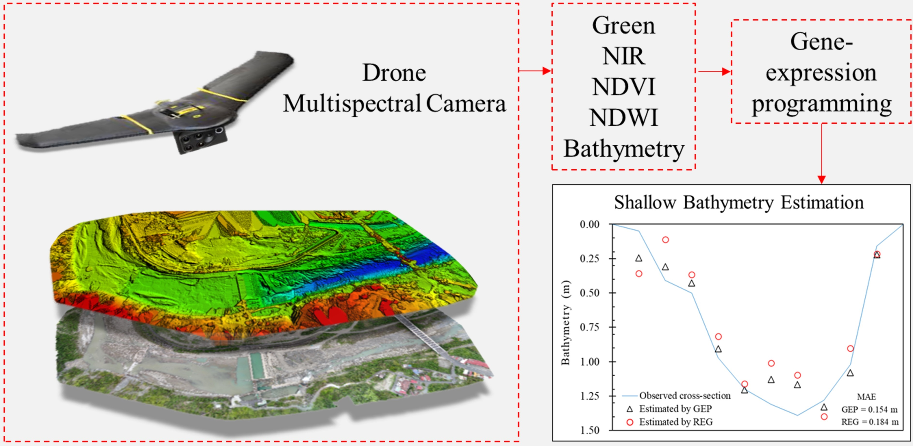
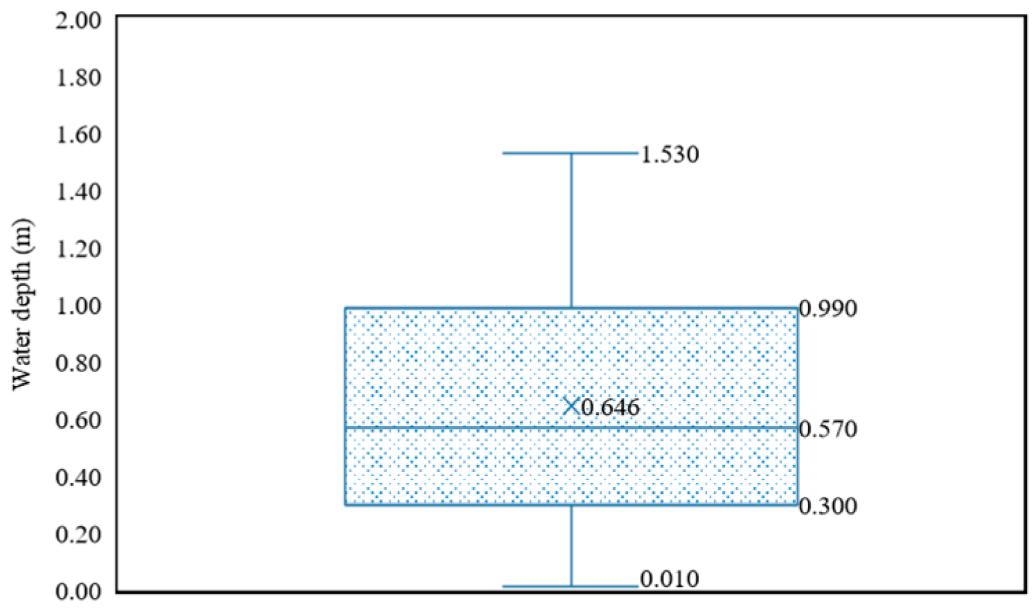
:The river cross-section elevation data are an essential parameter for river engineering. However, due to the difficulty of mountainous river cross-section surveys, the existing bathymetry investigation techniques cannot be easily applied in a narrow and shallow field. Therefore, this study aimed to establish a model suitable for mountainous river areas utilizing an unmanned aerial vehicle (UAV) equipped with a multispectral camera and machine learning-based gene-expression programming (GEP) algorithm. The obtained images were combined with a total of 171 water depth measurements (0.01–1.53 m) for bathymetry modeling. The results show that the coefficient of determination (R2) of GEP is 0.801, the mean absolute error (MAE) is 0.154 m, and root mean square error (RMSE) is 0.195 m. The model performance of GEP model has increased by 16.3% in MAE, compared to conventional simple linear regression (REG) algorithm, and also has a lower bathymetry retrieval error both in shallow (<0.4 m) and deep waters (>0.8 m). The GEP bathymetry retrieval model has a considerable degree of accuracy and could be applied to shallow rivers or near-shore areas under similar conditions of this study.

1. Introduction
The river cross-section is an essential parameter in water resources planning, hydraulics engineering, flow discharge modeling, ecological assessment, and river management [1,2,3,4,5,6,7,8,9,10]. In a general survey, the cross-sections are covered by a water body, thus, the investigators have to measure the distance from water surface to the riverbed, i.e., bathymetry. Typically, bathymetry is directly investigated using water-contact equipment, such as rope [3], lead fish [11], real-time kinematics (RTK) [12], and an acoustic doppler current profiler (ADCP) [7]. These kinds of bathymetry observation methods have a very high accuracy for mapping cross-sections, but the investigators need to carry heavy and expensive equipment to the field and take several hours or even days to collect the data [13], which makes survey updates rare or allows them to be conducted only on the sites of special interest [14]. Therefore, recently, many scholars have used remote sensing (RS) techniques, e.g., satellite or unmanned aerial vehicle (UAV), to retrieve river bathymetry data [8,15,16,17,18,19].
In recent RS-based bathymetry retrieval studies, Hernandez et al. [15] used light detection and ranging (LiDAR) to measure the seabed topography of La Parguera Nature Reserve in 2016. Worldview 2 (WV2) satellite image data, simple linear regression (REG) concept-based algorithm, and bands’ ratios of the satellite spectrum were used to retrieve water depth. The research results show that the root mean square error (RMSE) at 1 to 10 m is 1.260 m and the atmosphere, water quality, and turbidity have an impact on the accuracy of water depth retrieval.
Kim et al. [17] conducted a water depth survey using an UAV in 2019. The authors combined this with principal component analysis (PCA) to select the high influence spectral bands and then used REG, artificial neural network (ANN), and geographically weighted regression (GWR) algorithms to develop a water depth retrieval model. The coefficient of determination (R2) of REG, ANN, and GWR were 0.587, 0.595, and 0.851, respectively. The results indicated that the GWR model has certain accuracy for water depth retrieval and the choice of spectral band has an influence on the retrieval results.
Kasvi et al. [16] conducted a water depth retrieval study of the Pulmanki River, Finland in 2019. ADCP, REG, and structure from motion (SfM) developed from UAV aerial photography were used for modeling. The results show that ADCP has the best water depth measurement accuracy with mean absolute error (MAE) ranging from 0.030 m to 0.070 m, followed by REG (0.050–0.170 m) and SfM (0.180–2.980 m). The mean errors (ME) were similar and were in the order of ADCP (−0.030 m to 0.000 m), REG (−0.170 m to 0.020 m), and SfM (−0.440 m to 3.200 m). The author also points out that the error from image retrieval is similar to ADCP water depth measurement. Owing to the inability of ADCP to measure the 0 to 0.2 m shallow water depth, the cost of image retrieval water depth is considerably lower than that of ADCP, and given the lack of data, therefore, the image retrieval method should be used to estimate water depth under the suitable conditions of use.
Janowski et al. [18] developed a novel methodological approach to assess the suitability of airborne LiDAR bathymetry for the auto-classification and mapping of the seafloor based on ML classifiers in 2022. The application results show that the random forest algorithm has the best performance in scenarios and the overall accuracy in all scenarios ranged from more than 75% to 91%, with a median of 84%.
Although the abovementioned state-of-the-art techniques show a reasonable and reliable bathymetry modeling ability, they are mainly established for the application of wide areas and huge scales, e.g., wide rivers [9,16,20,21], lakes [5], or oceans [10,18,19,22]. Additionally, due to the limitation of satellite spatial and temporal resolution and the influence of cloud cover, most of the research results are only applicable to large sections and high-water-depth areas [23]. The riverbed sections of a large number of small and shallow rivers cannot be reasonably retrieved, and there are spatial resolution and observation frequency limitations in estimating water depth via satellite. Therefore, the existing bathymetry retrieval models are not easy to apply in regions which have narrow and shallow conditions with rapidly changing morphology [7] like the mountainous rivers in Taiwan.
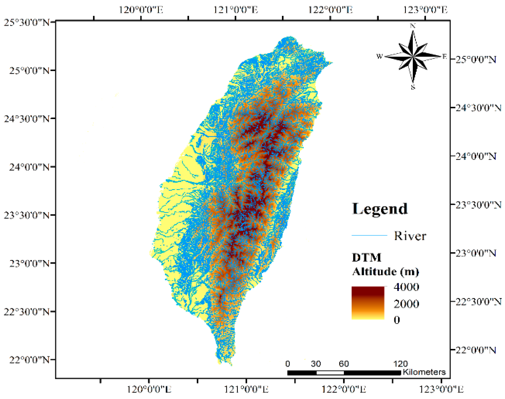
Taiwan is located in a typhoon-prone area with steep topography, rainfall is uneven during high and low water periods, and the flow rate varies considerably; therefore, the river section changes frequently, and the information of section surveys needs to be updated frequently [2,6]. Nevertheless, it is not easy to survey the river section directly with specific bathymetry, i.e., water depth. In addition, the rivers of Taiwan are predominantly in mountainous areas, and there are 131 named rivers in Taiwan, and more than 1000 submerged streams and wild streams, which are narrow and shallow (Figure 1). Under the circumstances of the bathymetry investigation in narrow and shallow river, the rapid development of UAV and advanced machine learning (ML) algorithm in recent years can possibly compensate for the lack of satellite image water depth retrieval. Samboko et al. [9] reviewed a study on the use of UAVs for river surveys and noted that UAVs can carry sensors to dangerous or inaccessible areas for surveys, and calibration can be conducted with relevant models developed to improve the applicability of this method. Moreover, Ashphaq et al. [19] reviewed over 100 research articles of satellite-derived bathymetry (SDB) retrieval models from past 50 years; the authors indicated that machine learning (ML) algorithms have a better modeling performance in the bathymetry where water depth is less than 20 m but require more relative studies for an applicability evaluation.
For there are many narrow and shallow rivers in Taiwan’s mountainous area and the riverbed changes frequently; manually investigating the river cross-section is difficult, and the applicability of the existing RS-based bathymetry retrieval model in shallow and narrow area are still unknown. Therefore, the authors aimed to link the gap between practical needs and the shortage of the existing bathymetry retrieval models by the following objectives in this study:
- (1)
- using UAV with multispectral camera to capture images and surveyed cross-section under shallow bathymetry conditions;
- (2)
- applying a ML algorithm to establish a water depth retrieval model for the rivers of Taiwan’s mountain area, which has yet been found in related studies;
- (3)
- encrypting the established model to Python-based program for further application, which can be used to simulate water depth for the shallow river or near-shore areas that are not easily measured under similar conditions as this study, where the water depth could be estimated by multispectral sensor mounted on the UAV.
2. Materials and Methods
2.1. Study Area
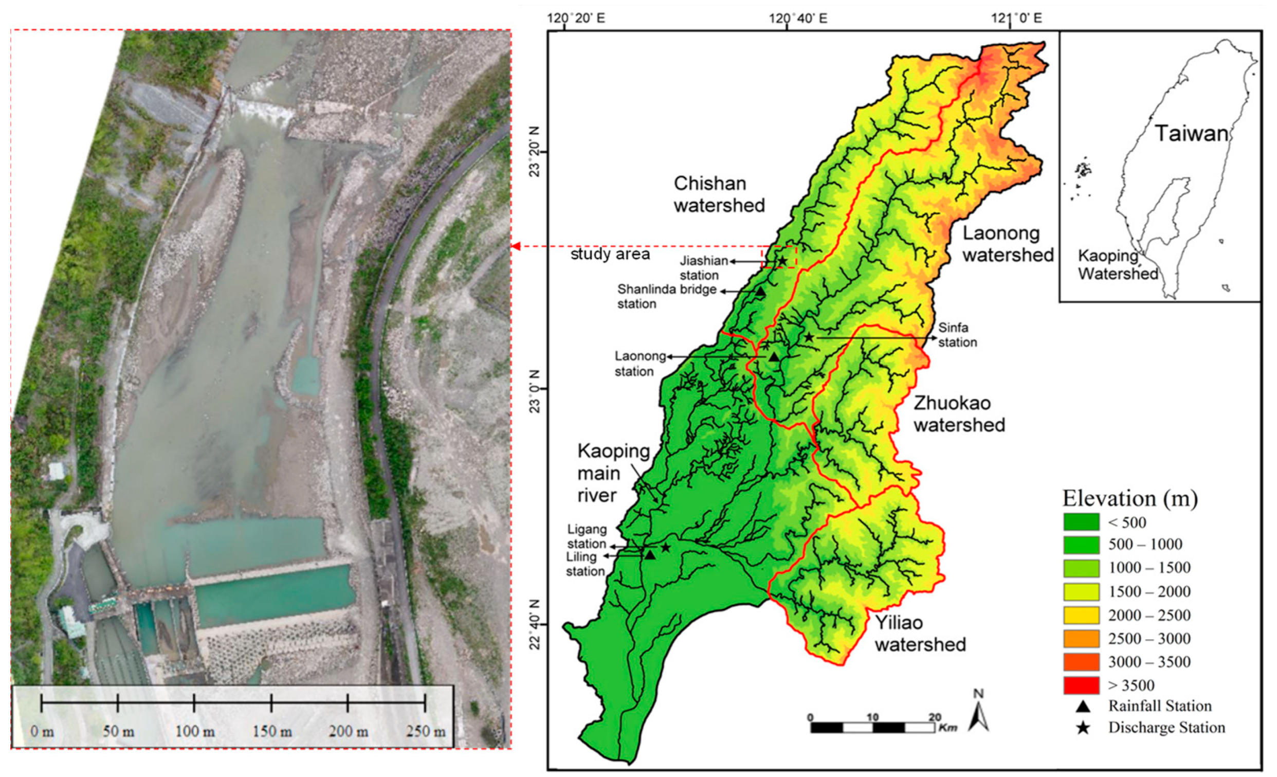
The study area is in the upstream of the Jiashian river weir section in Chishan River sub-watershed of the Kaoping River catchment (Figure 2) [24], which is built for supplying 0.3 million m3 of water per day on average for public and industrial use in Kaohsiung City, Taiwan, and providing 0.8 million m3 of water per day to the Nanhua Reservoir [25].
The river section is a typical mountainous river in Taiwan, with a river width of approximately 150 m, an elevation of 245 m, and a catchment area of 404.6 km2. In this location, the average annual rainfall is 2794.4 mm with an abundance of rainfall occurring in the wet season (May to October), as opposed to the dry season (November to April). From 2005 to 2007, the total rainfall averages in the dry and wet seasons were 235.9 and 2558.5 mm, respectively. It can be seen that the rainfall distribution at the location is unevenly distributed between the two seasons, which causes the flow discharge during the wet season to be approximately 90% of the annual total amount (1.14 billion m3). Moreover, based on the suspended sediment concentration (SSC) observations in the river section in the dry and wet seasons in 2003, the average SSC is 5.2 mg/L and 65.5 mg/L [26]. However, in 2009, typhoon Morakot caused an extreme rainfall event (1029 mm in 24 h), which lead to catastrophic flow discharge to occur in the Chishan River. The recorded flow discharge was 9308 m3/s in contrast to the designed 200 years return period flow discharge of 8380 m3/s, therefore, almost all of the hydraulic constructions were destroyed [27]. After the typhoon event, the river’s characteristics, especially SSC, changed to 129.3 mg/L in the dry season and 491.1 mg/L in the wet season in 2018, and the high SSC also caused a significant change in the river morphology and rapid changing river cross-section [1].
2.2. Bathymetry Investigation
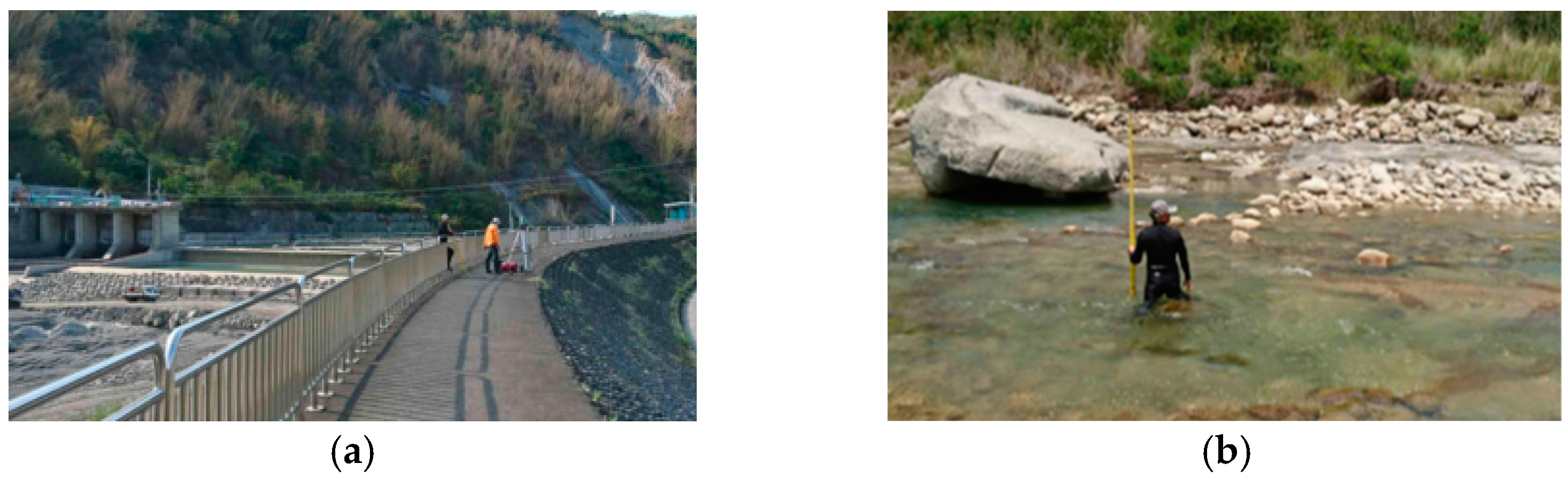
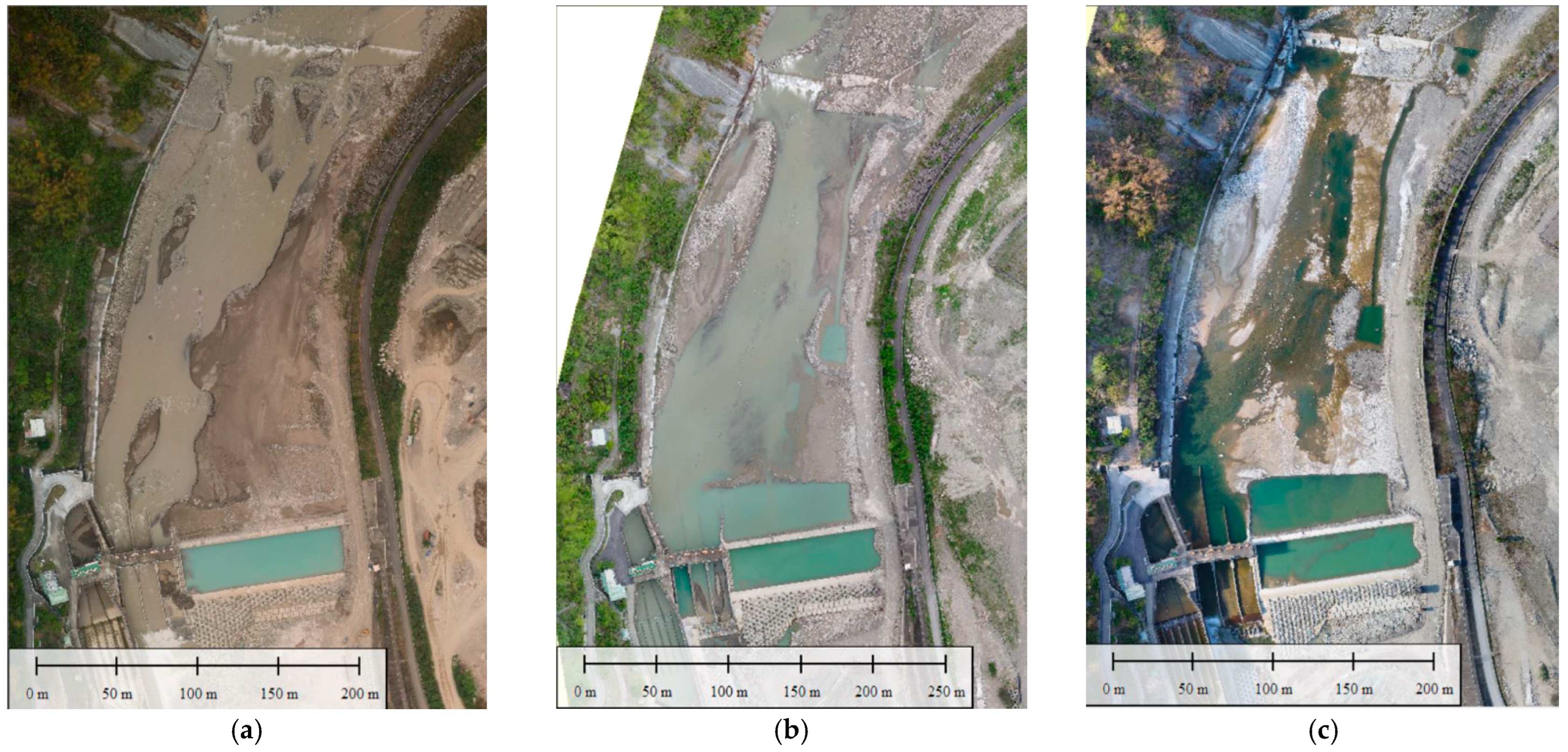
The Trimble R6-II RTK GPS was used for measuring the water depth of the upstream cross-section of the Jiaxian weir. In order to avoid the mountainous orographic precipitation and its high flow discharge occuring during the observation at the end of the wet season (after October), the experiments were conducted during the end of the dry season on 6 April 2016, 10 April 2017, and 2 May 2017. The static vertical accuracy of the equipment was up to ±5 + 1 ppm RMS, which meets the requirements of river cross-section surveys. The photos taken during the investigation are shown in Figure 3. It should be noted that the flow channel in the three observations was not always in the same position, and the color of the water, i.e., turbidity, was also different. The observation took place after a rainfall event on 6 April 2016, which has more sediment in the flow. In the observation, the submerged topographic change points were used as survey points, the surveyed bathymetry points were marked in Figure 4, and the data distribution is shown in Figure 5.
2.3. UAV and Multispectral Camera
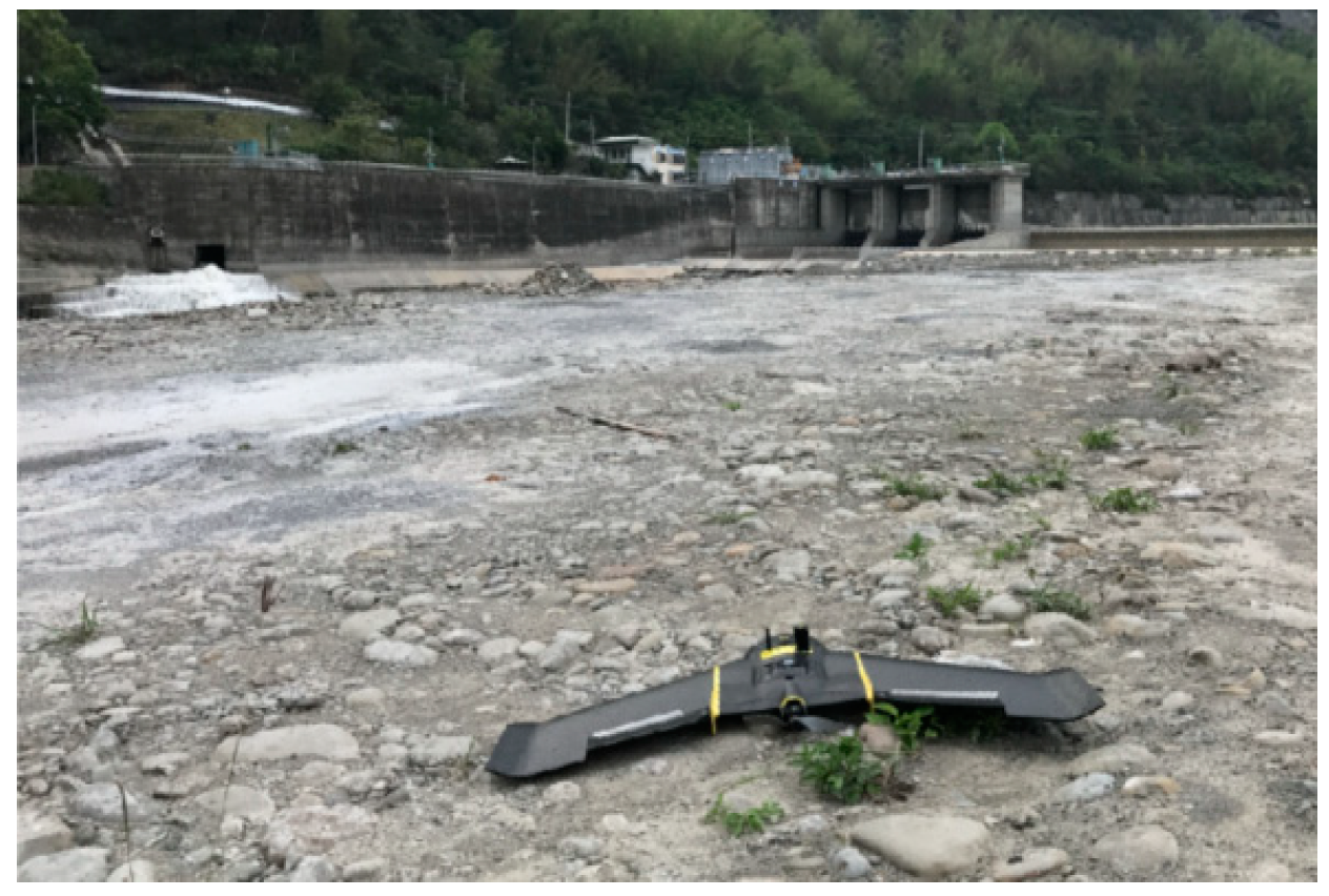
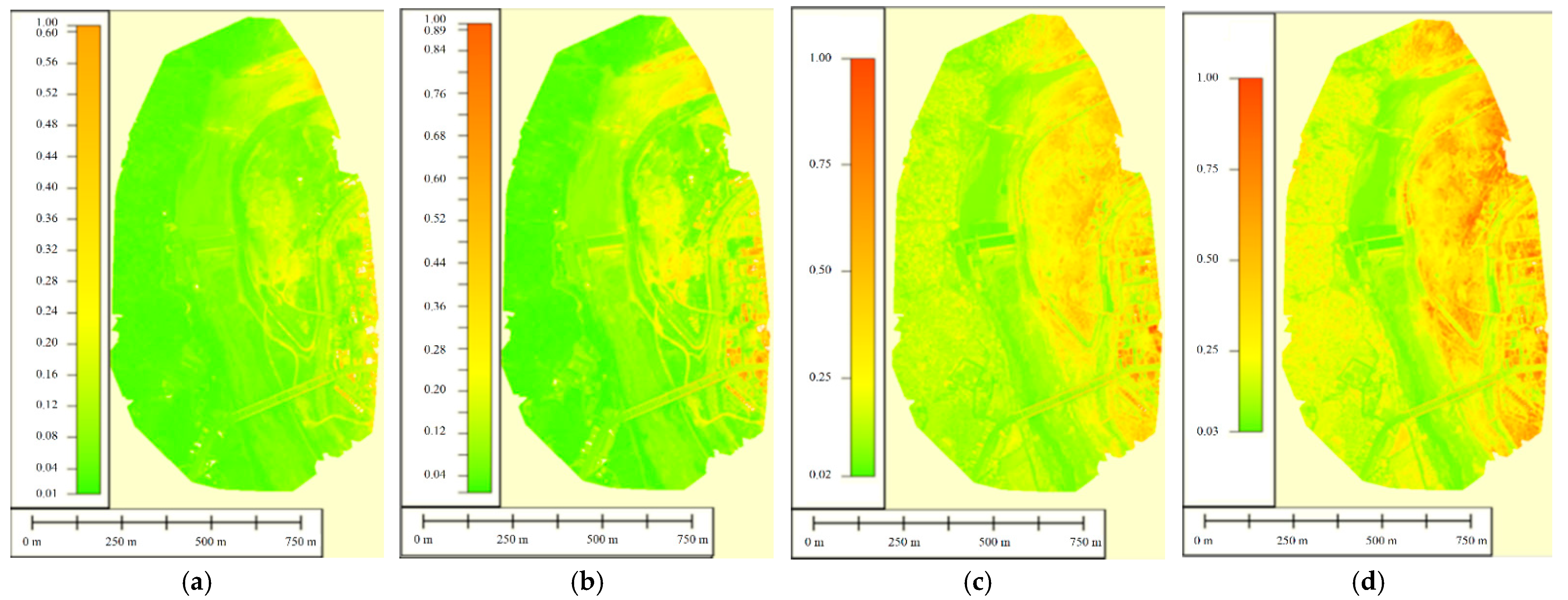
The aerial camera carrier is senseFly Ebee+ (Figure 6), which was equipped with a Parrot Sequoia multispectral camera with a spectrum of green (550 ± 40 nm), red (660 ± 40 nm), red edge (735 ± 10 nm), and near-infrared (NIR, 790 ± 40 nm). In each flight mission, the aerial altitude was about 100 m and the ground resolution was 17.12 cm. The number of aerial photographs was 772 to 1076 for a single cruise, with three flights taken on 6 April 2016, 10 April 2017, and 2 May 2017 (Figure 7, Table 1). Wind conditions and flight stability analysis are unavailable in this study. After obtaining the image data, Pix4D software was used to perform image stitching, control point correction, and normalized difference vegetation index (NDVI) [28], Equation (1), and the normalized difference water index (NDWI) calculations [29], Equation (2). The spectral information and indices value distribution including maximum, minimum, average, and standard deviation, obtained in the study are listed in Table 2. The spectral images, including green band, red band, red edge band, NIR band, and point cloud, generated from Pix4D of the study area are shown in Figure 8 and Figure 9.
where NDVI is the normalized difference vegetation index, NDWI is the normalized difference water index, NIR is the near-infrared reflection, RED and Green are the red and green reflections, respectively.
2.4. Data Processing
A total of 171 matched water depth-spectral data were obtained, near-infrared reflection (NIR), green, NDVI, and NDWI were used as inputs to the water depth retrieval model, referring to previous studies [12,22,30,31], the measured water depth data was used as the output.
All of the data were normalized as Equation (3) and randomly sorted, referring to [32,33]. Of the total data, 70% were used as the training dataset to build the model (n = 138), and then 30% of the remaining data (n = 33) were used for the model test. The results of the t-test after the classification of the datasets are presented in Table 3. The results show that the characteristics of the classified datasets did not reach statistically significant differences.
where x refers to the spectral and water depth data; xmax and xmin are the maximum and minimum of the dataset, respectively; xnorm refers to the value after the data x normalization.
2.5. Development of Water Depth Retrieval Model
Gene-expression programming (GEP), an advanced machine learning algorithm, was used to develop water depth retrieval model. The results were compared with simple linear regression (REG) based simulations, which is commonly used in previous studies [15,23,34], to evaluate the advantages and disadvantages of the GEP model.
2.5.1. Gene-Expression Programming (GEP)
GEP is an algorithm that combines the advantages of genetic algorithm (GA) for linear symbolic coding and genetic programming (GP) for solving nonlinear complex problems. The concept of GEP is to start with an initial race and to evolve toward a predetermined goal through a continuous evolutionary process (including selection, replication, mating, mutation, adaptation, retrieval, and conversion). Besides improving the shortcomings of GA premature convergence and GP combination explosion, the evolutionary speed of GA is 100 times higher than that of GA and GP [35].
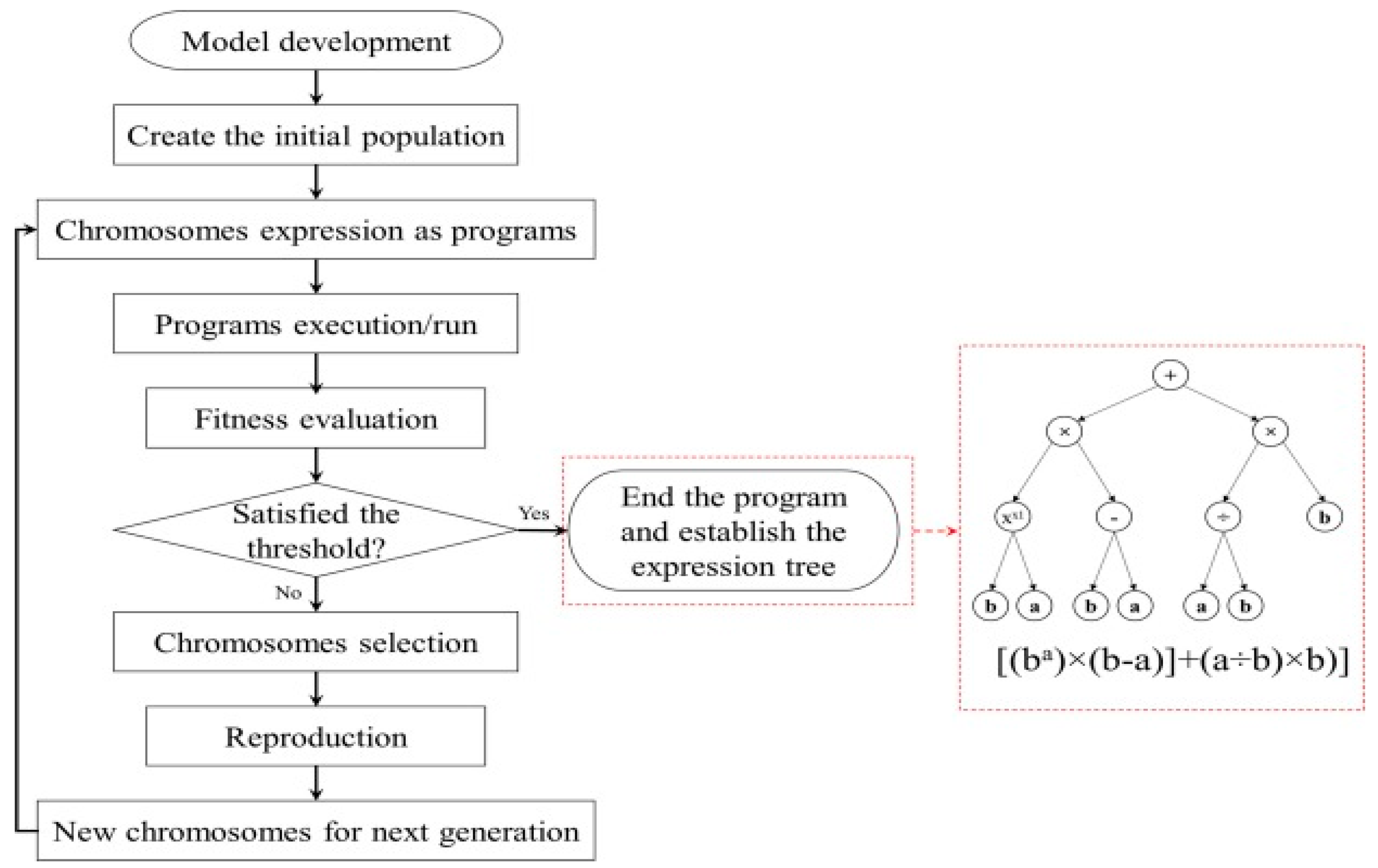
GEP encoding rules are the same as GA algorithm, both are encoded in equal linear symbols to form “genes”. Then one or more genes are combined to form a chromosome. Among them, different types of nodes can be placed at the gene location, including function and terminal nodes. The function nodes can be arithmetic or logical operands and comparison operands (+, −, ×, ÷, ln, sin, cos, <, =, >… etc.), and the terminal nodes can be custom variables or constants. The structure of each chromosome is at least divided into head and tail sizes, and the head size can contain function nodes and terminal nodes, while the tail size has only terminal nodes, and the number of tail genes is related to the head size. A tree structure, called a gene expression trees (ETs), can be built based on the chromosome of gene binding, and the expression of the chromosome can be obtained according to the bottom-up and left-to-right rules, as shown in Figure 10 [36]. Referring to Wang et al. [37], the operands used in this study were +, −, ×, ÷, ln, sin, cos, <, =, >…, conjunction function was minimization (min), chromosome number used for modal training was 50, head size was 10, gene number was 2, adaptation function was mean absolute error (MAE), and the number of iterations of modal training was 100,000.
2.5.2. Simple Linear Regression (REG)
REG is a conventional linear algorithm, which is used as the contrast of GEP algorithm in this study. The training dataset and testing dataset is the same as GEP.
where xi is the ith input, α is the parameter, β is an intercept of the regression, and ε is the error term.
2.6. Model Accuracy Evaluation
The model simulation results can be evaluated via the calculation of evaluation metrics. The coefficient of determination (R2), absolute error (AE), MAE, ME, and RMSE were used to evaluate the rationality of the model Equations (5)–(8) in this study. Herein, R2 is the ability to evaluate the ratio of the variation value of the model to all variation values. The larger R2 is, the more the model can explain the proportion of all variation values; and the closer R2 is to 1.0, the more the model has the ability to explain. However, since R2 is susceptible to extreme values, simulation results may differ greatly from the actual value when R2 is close to 1. Therefore, error quantity is needed to evaluate the advantages and disadvantages of the model and analyze the main range of error.
where R2 is the coefficient of determination, is the predicted value in ith datum, is the observed value in ith datum, is the average of the observations, n is the number of actual observations, MAE is the mean absolute error, AE is the absolute error, ME is the mean error, and RMSE is the root mean square error.
3. Results
3.1. Simulation Results and Accuracy Evaluation
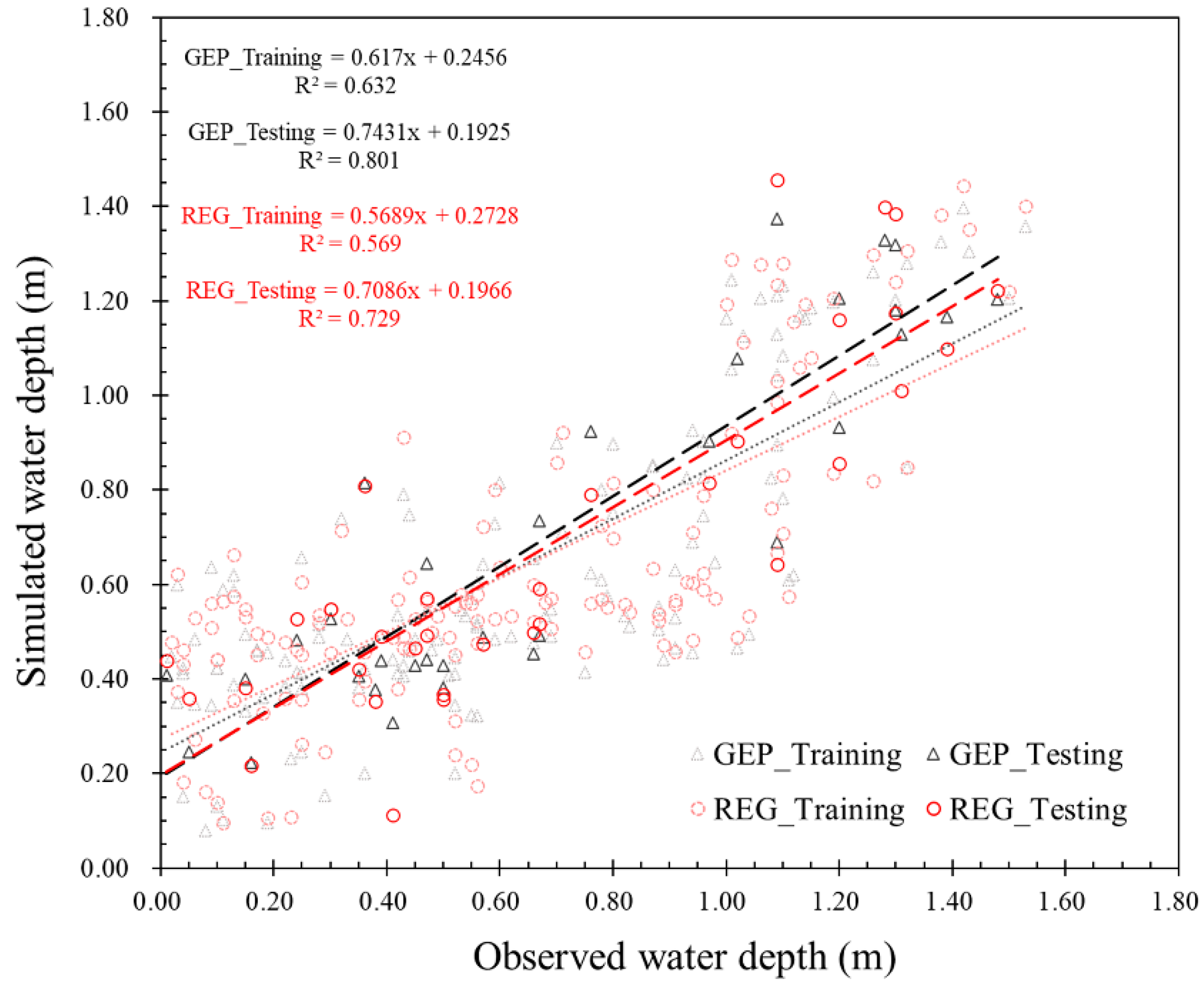
Figure 11 shows the water depth results simulated according to the two models and Table 4 shows the accuracy evaluation results. As observed, GEP and REG have similar performance in model training and test stage, while the GEP algorithm may have better performance in R2, MAE, and RMSE than the linear-based REG due to its ability to handle complex dimensional problems and learning. It should be mentioned that the reason why the different quality of the models, partitioning, or structure of the models is not discussed is due to the relatively small dataset of this study.
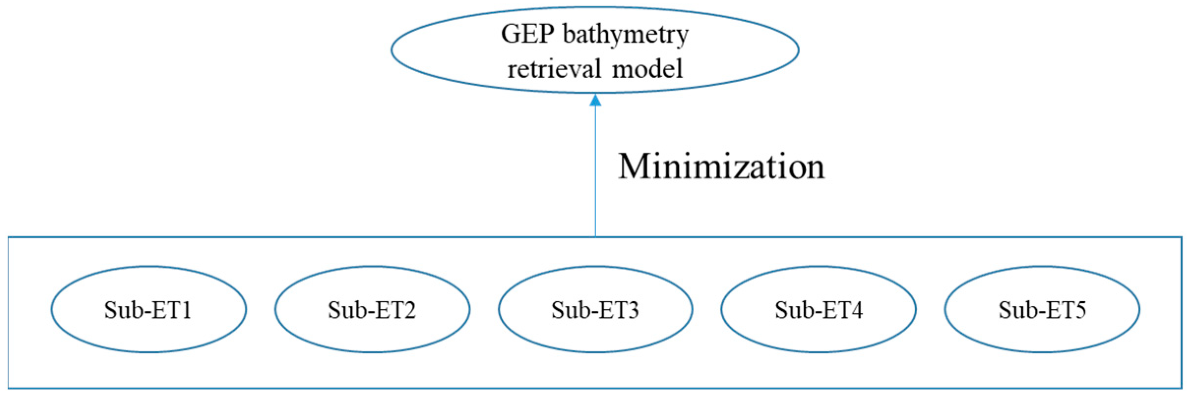
In ME, although the value of REG was small (−0.008 m), it was not significantly different from that of GEP (0.012 m). The bathymetry retrieval model developed by REG is shown in Equation (9). The GEP model (Figure 12), which is composed of five sub-ETs (Appendix A, Figure A1, Figure A2, Figure A3, Figure A4 and Figure A5), is compiled in Python language, and the program is enclosed in Appendix B.
where a, b, c, and d, respectively, are the constants of the REG bathymetry retrieval model. In this study, a , , c, d, and e.
3.2. Error Evaluation
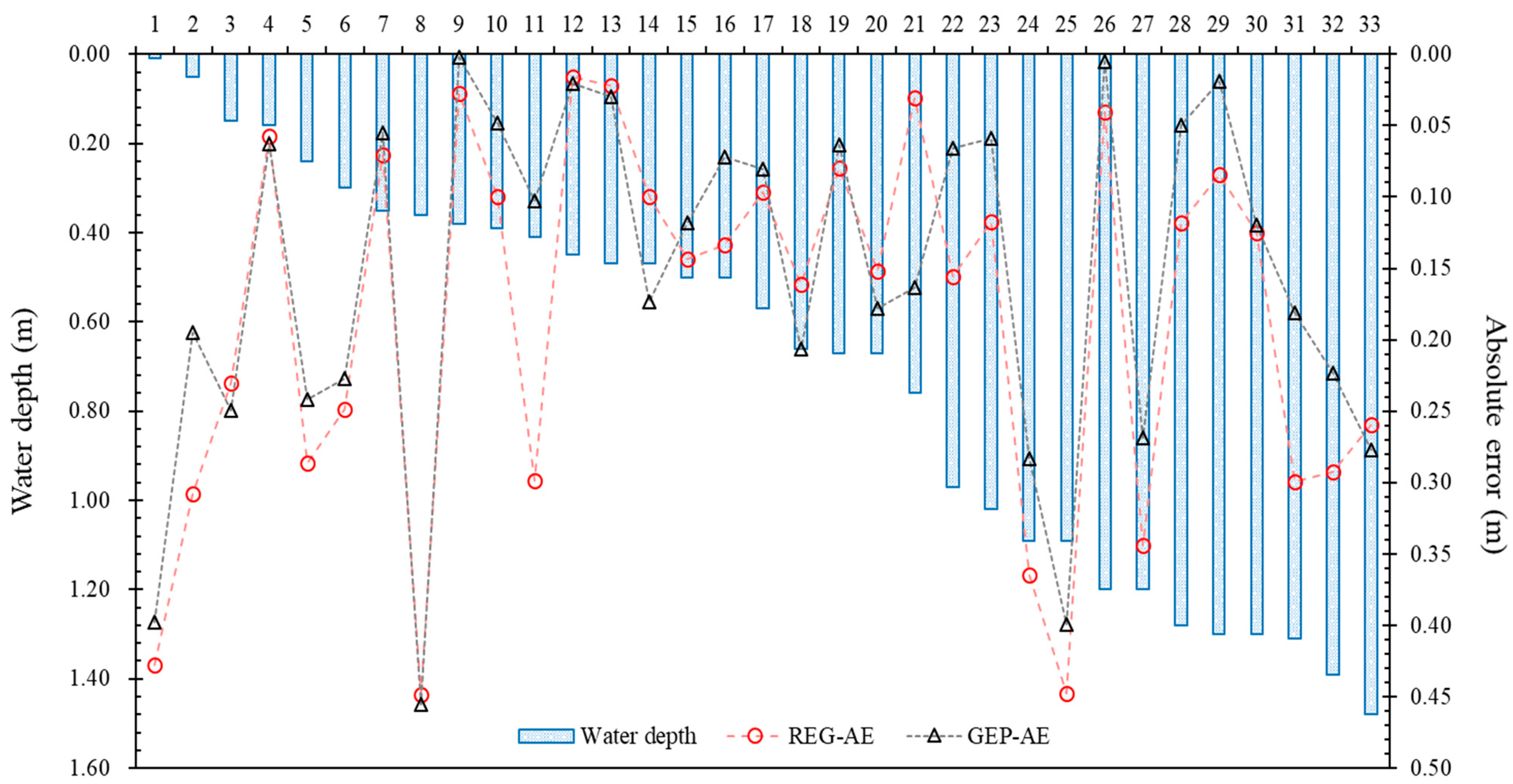
The observed water depth and the retrieval AE of the two models for the test dataset are compared and discussed. As shown in Figure 13 and Table 5, the simulation performance of REG for shallow water (<0.4 m) and deep water (>0.8) is generally poor compared with that of GEP model, and the retrieval error in the middle water depth [0.4 m, 0.8 m] is close to that of the GEP model. It should be mentioned that regarding all of the enormous errors, i.e., datum numbers, 1, 8, 24, 25, 27, and 33, were observed after a rainfall event in a turbid water condition on 6 April 2016. Therefore, the numerous errors in the near-surface and bottom layers may be caused by light penetration, scattering variation, water quality, or riverbed composition [5,16,38].
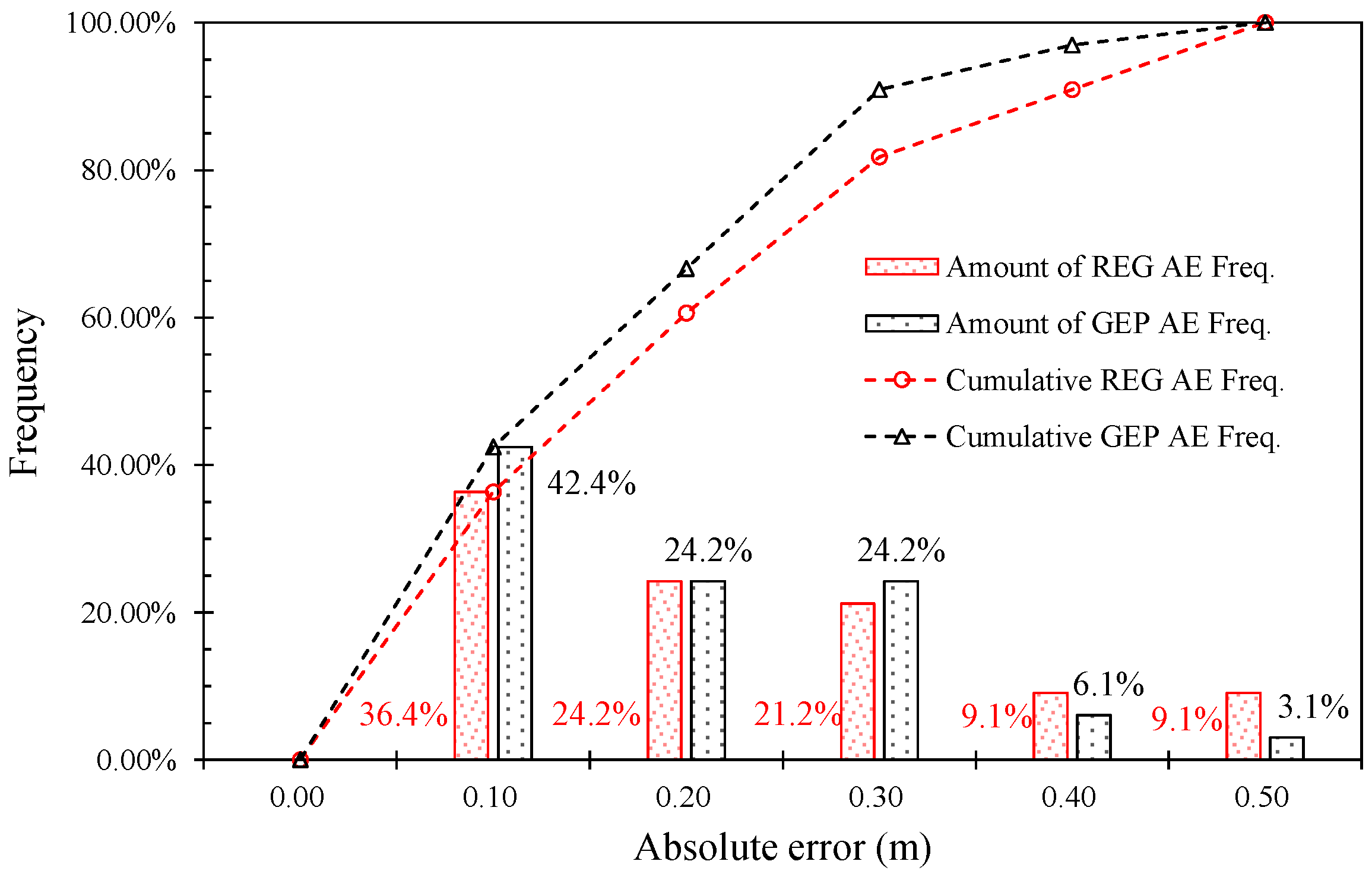
As to the statistical part of error, the number of AE error was classified at an interval of 0.1 and then counted in this study, as shown in Figure 14. It can be seen that the AE of approximately 90.9% water depth retrieval in GEP is less than 0.30 m, which is better than that in REG (81.8%). In the percentage of AE > 0.50 m, GEP (3.1%) is also lower than that in REG (9.1%), which indicates that the GEP algorithm can avoid large errors in water depth retrieval. This result is of great significance to retrieval of shallow water depth as it can improve the rationality of the model retrieval of water depth.
4. Discussion
In this study, the water depth reverse research model was developed for the mountainous rivers in southern Taiwan. The results show that huge absolute errors occur in the turbid water, which is similar to the findings of [5,16,38]. Furthermore, this study compares the modeled results and errors with relevant studies. Although the study area, data source, and data range were different from other studies and the results could not be directly compared, the water depth retrieval results of each study can be used to slightly evaluate the difference in accuracy of the water depth evaluation of different models.
As shown in Table 6, in the MAE section, the GEP model developed in this study exhibits a higher retrieval error (0.154 m) than that (0.112 m) of the REG model developed via [16]; the value is higher than MAE (0.053 m) obtained at 0.20 to 1.50 m water depth via the contact measurement with ADCP but lower than that (0.740 m) of the water depth obtained using the SfM method. In ME, the retrieval error (REG = −0.008 m, GEP = 0.012 m) of this study is similar to that of the ADCP contact measurement result of and better than the water depth results obtained via telemetry combined with the deep learning or random forest algorithm [16,21,39,40]. Finally, in the RMSE comparison section, GEP outperformed the simulation results of the water depth retrieval model developed using machine learning [23,34,40,41] or linear algorithms [15,23,34] in previous studies, which indicates that the GEP water depth retrieval model developed in this study has a certain degree of accuracy. Considering that the UAV has the ability to quickly survey a large area according to the user’s needs and the MAE error is of the same magnitude as ADCP but the price is only 10% of ADCP, it should be able to meet the shallow water depth survey requirements of mountainous rivers in Taiwan.
The established bathymetry model showed a certain degree of retrieval accuracy of the study area. Nevertheless, the authors should mention that the water depth retrieval model is influenced by many factors, including light sources, turbidity and the penetration range [18,39], water composition, underwater vegetation cover, riverbed composition [16], and other parameters which may inhibit acoustic waves like salinity, temperature, etc. [19]. Therefore, the evaluation of the water depth near the surface or near the bottom layer may cause low accuracy, but it can be seen from the comparison of error distribution that GEP has the ability to avoid significant error. Additionally, compared with other studies, high-resolution multispectral images are adopted in this study. Therefore, the differences in the resolution of images, types of aircraft, and multispectral camera bands may affect the retrieval results. In the actual application, the model should be selected based on the development of the model, using the accuracy requirements and the results of current surveys.
5. Conclusions
Due to the rivers in the mountainous areas of Taiwan being often narrow and shallow and under the influence of extreme rainfall caused by climate change, the scour and deposition of riverbeds change rapidly, and how to quickly obtain a reasonable riverbed cross-section has become a topic faced in river engineering. In this study, an UAV equipped with a multispectral camera was used to shoot the high-resolution multispectral images of Taiwan mountainous streams for quickly obtaining a river cross-section. The bathymetry retrieval model is developed using the GEP and REG algorithms. The results show that the MAE performance of GEP has increased by 16.3%, compared to the REG model. For the further comparison with relevant studies, the accuracy of the GEP model is close to or better than related studies using images to retrieve water depth and can avoid the occurrence of significant error. GEP is suitable for the water depth retrieval of rivers in mountainous areas in Taiwan and can be used for river management planning and disaster prevention management evaluation or the shallow shores of shallow rivers or near-shore areas that are not easily measured under similar conditions as this study.
That being said, in practical applications, considering the basis of model development, accuracy requirements, and field survey results when choosing a suitable model remains necessary. This study only discusses the capability of the GEP algorithm applied to shallow water river in the southern mountainous region of Taiwan and indicates that its retrieval accuracy is sufficient for the water depth evaluation of the study area, which can be used as an alternative when water depth is not available on site, so it cannot be fully compared with other case studies. For further research, it is suggested that researchers might conduct more extensive case studies or meta-studies on the RS water depth retrieval technology, e.g., deep learning algorithms, generalized additive model (GAM), and decision trees.
Author Contributions
Conceptualization, C.-H.L.; methodology, C.-H.L. and C.-L.C.; software, L.-W.L.; validation, C.-L.C. and Y.-M.W.; formal analysis, L.-W.L. and C.-H.L.; investigation, C.-H.L.; resources, J.-M.L. and C.-H.L.; writing—original draft preparation, L.-W.L. and C.-H.L.; writing—review and editing, J.-M.L., Y.-M.W. and C.-L.C.; visualization, L.-W.L.; supervision, C.-L.C. and Y.-M.W.; project administration, J.-M.L. and C.-L.C.; funding acquisition, C.-H.L. All authors have read and agreed to the published version of the manuscript.
Funding
This research received no external funding.
Data Availability Statement
Not applicable.
Conflicts of Interest
The authors declare no conflict of interest.
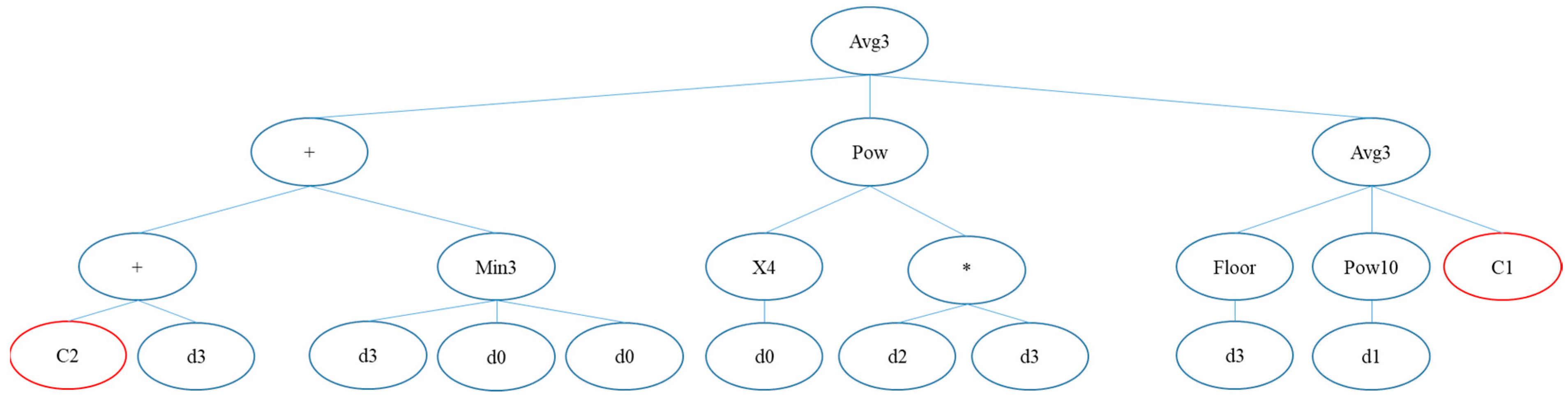
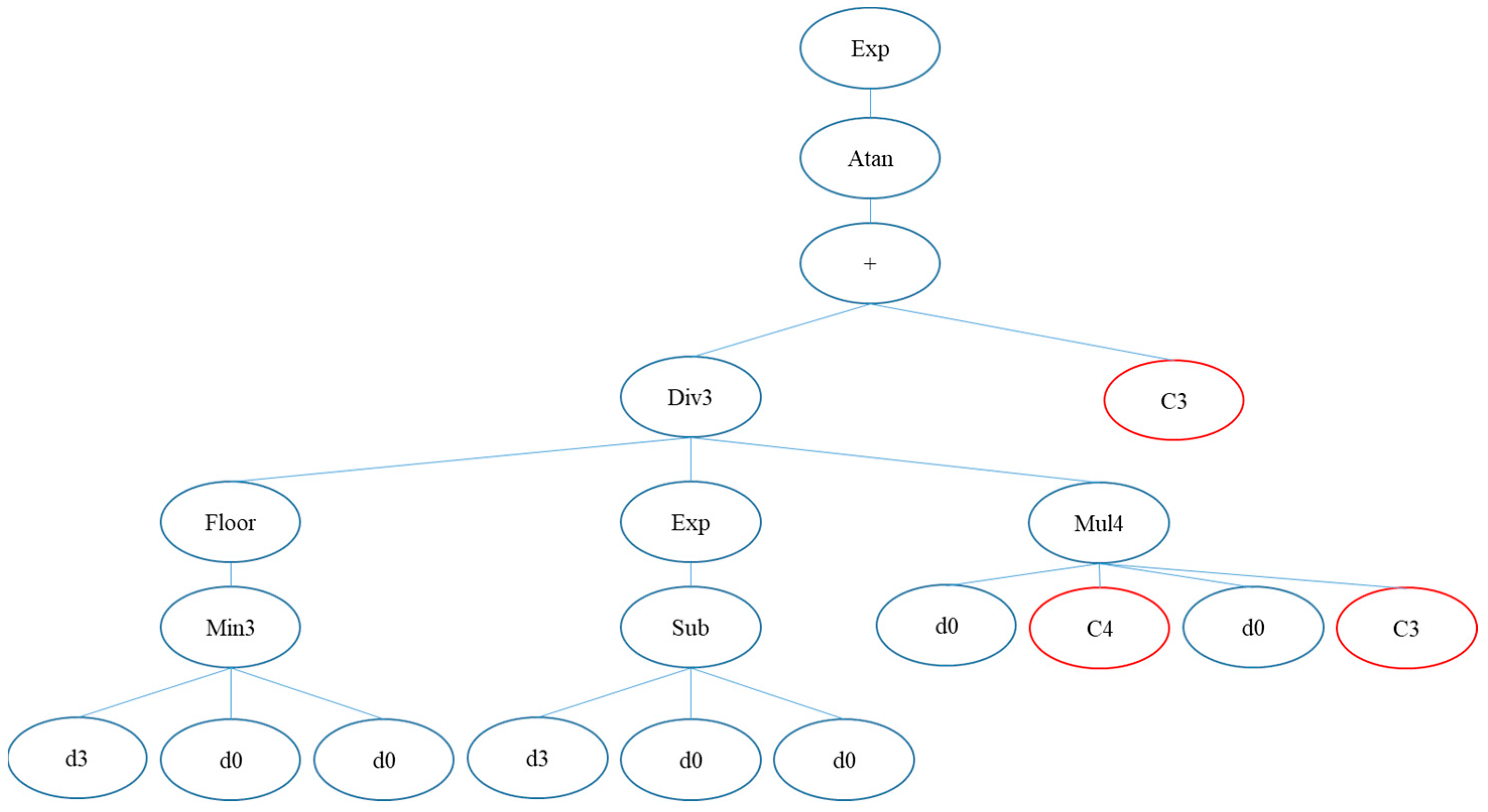
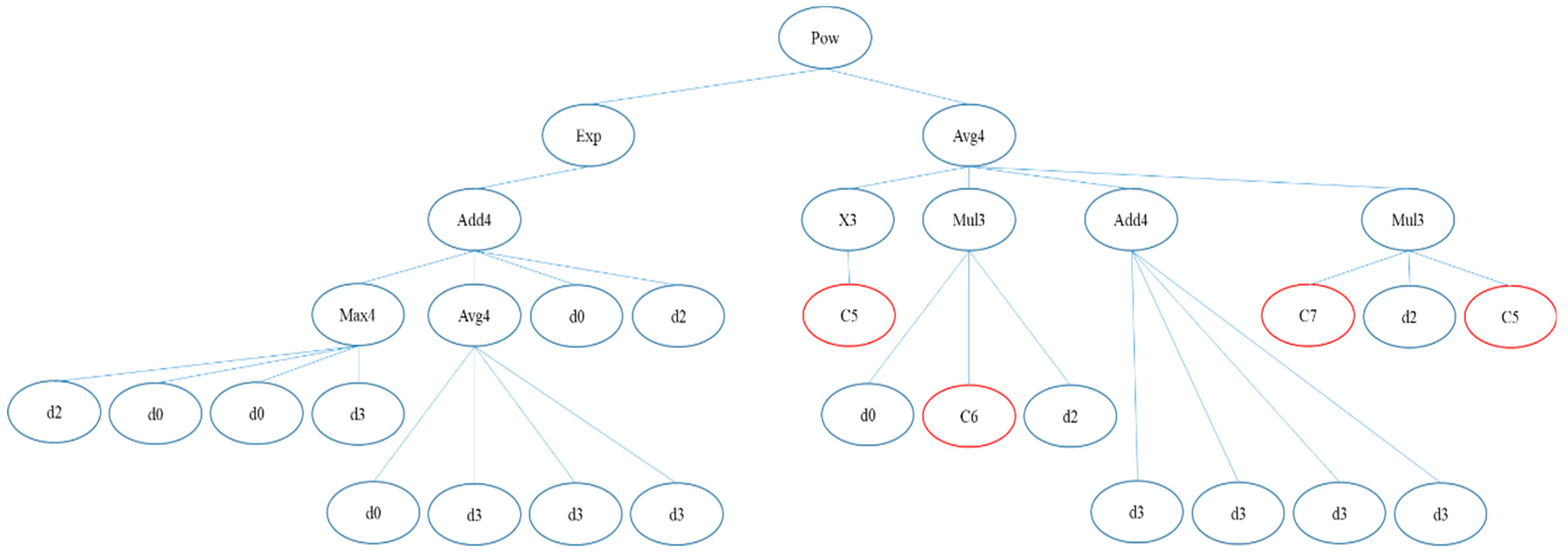
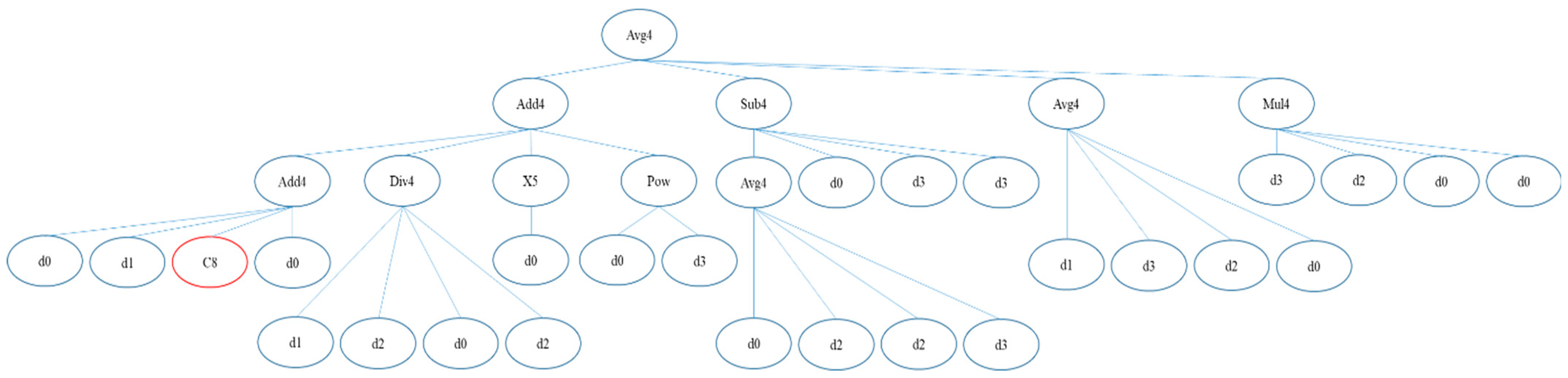
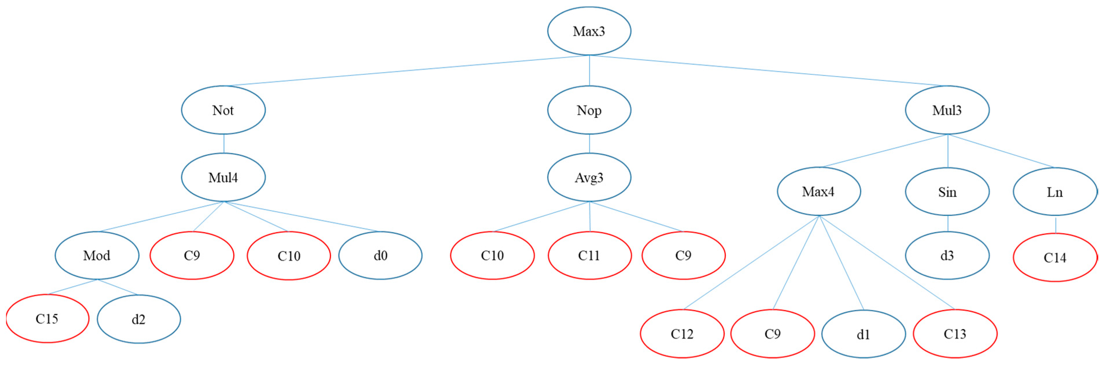
Appendix A. Sub-ETs of GEP Bathymetry Retrieval Model
Figure A1.
Sub-ET1 of GEP bathymetry retrieval model.

Figure A2.
Sub-ET2 of GEP bathymetry retrieval model.

Figure A3.
Sub-ET3 of GEP bathymetry retrieval model.

Figure A4.
Sub-ET4 of GEP bathymetry retrieval model.

Figure A5.
Sub-ET5 of GEP bathymetry retrieval model. Where, Avg is average function, Pow is power function, Nop is no operation, Min is minimize function, Max is maximize function, X3~5 is x to the power of 3~5, Floor is floor function, Pow10 is 10 to the power of x, Exp is exponential function, Atan is arctangent function, Mul is multiplication function, Div is division function, Add is addition function, Sub is subtraction function, Not is complement function, Mod is floating-point remainder function, Sin is sine function, Ln is natural log function, and C1 to C15 is constants, which can be found in Appendix B.

Appendix B. Python-Based Code for Shallow Water Depth Retrieval by UAV Imagery
#------------------------------------------------------------------------
# UAV and Multispectrum: senseFly Ebee+, Parrot Sequoia
# Study area: Jiashian weir, Kaohsiung County, Taiwan
# Data range on water depth: 0.01m to 1.53m
# d[0]: NIR; d[1]: Green; d[2]: NDVI; d[3]: NDWI
#------------------------------------------------------------------------
from math import *
def bathymetry(d):
C1 = 3.0629214683402; C2 = 7.44743097927145; C3 = −6.01210684838703;
C4 = 5.67636563981775; C5 = 5.26783952924083; C6 = 465.48597815585;
C7 = 59.4521367572932; C8 = −9.7882015442366; C9 = −3.5382776565035;
C10 = −8.9856119439729; C11 = −6.1264381847591; C12 = −5.0825760673849;
C13 = 4.88974384648924; C14 = 6.4059468784722; C15 = 1.63019287697989;
y = 0.0
- y = ((((C2+d[3])*min(d[3],d[0],d[0]))+pow(pow(d[0],4.0),(d[2]*d[3]))+((floor (d[3])+pow(10.0,d[1])+C1)/3.0))/3.0)
- y = min(y,exp(atan(((floor(min(d[0],d[2],d[0]))/exp((d[0]-d[2]-d[3]))/(d[0]*C4* d[0]*C3))+C3))))
- y = min(y,pow(exp((max(d[2],d[0],d[0],d[3])+((d[0]+d[3]+d[3]+d[3])/4.0)+d[0]+ d[2])),((pow(C5,3.0)+(d[0]*C6*d[2])+(d[3]+d[3]+d[3]+d[3])+(C7*d[2]*C5))/4.0)))
- y = min(y,((((d[0]+d[1]+C8+d[0])+(d[1]/d[2]/d[0]/d[2])+pow(d[0],5.0)+pow (d[0],d[3]))+(((d[0]+d[2]+d[2]+d[3])/4.0)-d[0]-d[3]-d[3])+((d[1]+d[3]+d[2]+d[0]) /4.0)+(d[3]*d[2]*d[0]*d[0]))/4.0))
- y = min(y,max((1.0-(gepMod(C15,d[2])*C9*C10*d[0])),(((C10+C11+C12)/3.0)), (max(C12,C9,d[1],C13)*sin(d[3])*log(C14))))
return y
def gepMod(x,y):
# The built-in function is incorrect for cases such as −1.0 and 0.2.
numSign = 0.0
if ((x/y) < 0):
numSign = −1.0
elif ((x/y) > 0):
numSign = 1.0
else:
numSign = 0.0
return x - (numSign * floor(abs(x/y))) * y
References
- G.R.W.M. Committee. The 2018 Annual Report on the Management and Implementation of Kaoping River Basin. 2019. [Google Scholar]
- Dadson, S.J.; Hovius, N.; Chen, H.; Dade, W.B.; Hsieh, M.-L.; Willett, S.D.; Hu, J.-C.; Horng, M.-J.; Chen, M.-C.; Stark, C.P.; et al. Links between erosion, runoff variability and seismicity in the Taiwan orogen. Nature 2003, 426, 648–651. [Google Scholar] [CrossRef] [PubMed]
- Dierssen, H.M.; Theberge, A.E. Bathymetry: Seafloor mapping history. In Coastal and Marine Environments; CRC Press: Boca Raton, FL, USA, 2020; pp. 195–202. [Google Scholar]
- Gustafsson, H.; Zuna, L. Unmanned Aerial Vehicles for Geographic Data Capture: A Review. Bachelor’s Thesis, School of Architecture and the Built Environment, Kensington, NSW, Australia, 2017. [Google Scholar]
- Heblinski, J.; Schmieder, K.; Heege, T.; Agyemang, T.K.; Sayadyan, H.; Vardanyan, L. High-resolution satellite remote sensing of littoral vegetation of Lake Sevan (Armenia) as a basis for monitoring and assessment. Hydrobiologia 2011, 661, 97–111. [Google Scholar] [CrossRef]
- Huang, M.Y.F.; Montgomery, D.R. Fluvial response to rapid episodic erosion by earthquake and typhoons, Tachia River, central Taiwan. Geomorphology 2012, 175–176, 126–138. [Google Scholar] [CrossRef]
- Kasvi, E.; Laamanen, L.; Lotsari, E.; Alho, P. Flow Patterns and Morphological Changes in a Sandy Meander Bend during a Flood—Spatially and Temporally Intensive ADCP Measurement Approach. Water 2017, 9, 106. [Google Scholar] [CrossRef] [Green Version]
- Munawar, H.S.; Ullah, F.; Qayyum, S.; Heravi, A. Application of Deep Learning on UAV-Based Aerial Images for Flood Detection. Smart Cities 2021, 4, 65. [Google Scholar] [CrossRef]
- Samboko, H.T.; Abas, I.; Luxemburg, W.M.J.; Savenije, H.H.G.; Makurira, H.; Banda, K.; Winsemius, H.C. Evaluation and improvement of remote sensing-based methods for river flow management. Phys. Chem. Earth Parts A/B/C 2020, 117, 102839. [Google Scholar] [CrossRef]
- Tamminga, A.; Hugenholtz, C.; Eaton, B.; Lapointe, M. Hyperspatial Remote Sensing of Channel Reach Morphology and Hydraulic Fish Habitat Using an Unmanned Aerial Vehicle (UAV): A First Assessment in the Context of River Research and Management. River Res. Appl. 2015, 31, 379–391. [Google Scholar] [CrossRef]
- Kostaschuk, R.A.; Church, M.A. Macroturbulence generated by dunes: Fraser River, Canada. Sediment. Geol. 1993, 85, 25–37. [Google Scholar] [CrossRef]
- Alevizos, E.; Alexakis, D.D. Evaluation of radiometric calibration of drone-based imagery for improving shallow bathymetry retrieval. Remote Sens. Lett. 2022, 13, 311–321. [Google Scholar] [CrossRef]
- Kammerer, E.; Charlot, D.; Guillaudeux, S.; Michaux, P. Comparative study of shallow water multibeam imagery for cleaning bathymetry sounding errors. In Proceedings of the MTS/IEEE Oceans 2001. An Ocean Odyssey. Conference Proceedings (IEEE Cat. No. 01CH37295), Honolulu, HI, USA, 5–8 November 2001; Volume 2124, pp. 2124–2128. [Google Scholar]
- Pacheco, A.; Horta, J.; Loureiro, C.; Ferreira, Ó. Retrieval of nearshore bathymetry from Landsat 8 images: A tool for coastal monitoring in shallow waters. Remote Sens. Environ. 2015, 159, 102–116. [Google Scholar] [CrossRef] [Green Version]
- Hernandez, W.J.; Armstrong, R.A. Deriving Bathymetry from Multispectral Remote Sensing Data. J. Mar. Sci. Eng. 2016, 4, 8. [Google Scholar] [CrossRef]
- Kasvi, E.; Salmela, J.; Lotsari, E.; Kumpula, T.; Lane, S.N. Comparison of remote sensing based approaches for mapping bathymetry of shallow, clear water rivers. Geomorphology 2019, 333, 180–197. [Google Scholar] [CrossRef]
- Kim, J.S.; Baek, D.; Seo, I.W.; Shin, J. Retrieving shallow stream bathymetry from UAV-assisted RGB imagery using a geospatial regression method. Geomorphology 2019, 341, 102–114. [Google Scholar] [CrossRef]
- Janowski, L.; Wroblewski, R.; Rucinska, M.; Kubowicz-Grajewska, A.; Tysiac, P. Automatic classification and mapping of the seabed using airborne LiDAR bathymetry. Eng. Geol. 2022, 301, 106615. [Google Scholar] [CrossRef]
- Ashphaq, M.; Srivastava, P.K.; Mitra, D. Review of near-shore satellite derived bathymetry: Classification and account of five decades of coastal bathymetry research. J. Ocean. Eng. Sci. 2021, 6, 340–359. [Google Scholar] [CrossRef]
- Bures, L.; Sychova, P.; Maca, P.; Roub, R.; Marval, S. River Bathymetry Model Based on Floodplain Topography. Water 2019, 11, 1287. [Google Scholar] [CrossRef] [Green Version]
- Jérôme, L.; Gentile, V.; Demarchi, L.; Spitoni, M.; Piégay, H.; Mróz, M. Bathymetric Mapping of Shallow Rivers with UAV Hyperspectral Data. In Proceedings of the Fifth International Conference on Telecommunications and Remote Sensing, Milan, Italy, 10–11 October 2016; pp. 43–49. [Google Scholar]
- Van-An, N.; Hsuan, R.; Chih-Yuan, H.; Kuo-Hsin, T. Bathymetry derivation in shallow water of the South China Sea with ICESat-2 and Sentinel-2 data. J. Appl. Remote Sens. 2021, 15, 044513. [Google Scholar] [CrossRef]
- Lee, C.B.; Traganos, D.; Reinartz, P. A Simple Cloud-Native Spectral Transformation Method to Disentangle Optically Shallow and Deep Waters in Sentinel-2 Images. Remote Sens. 2022, 14, 590. [Google Scholar] [CrossRef]
- Wu, C.-H.; Chen, S.-C.; Chou, H.-T. Geomorphologic characteristics of catastrophic landslides during typhoon Morakot in the Kaoping Watershed, Taiwan. Eng. Geol. 2011, 123, 13–21. [Google Scholar] [CrossRef]
- Wang, Y.-M.; Traore, S.; Kerh, T. Using artificial neural networks for modeling suspended sediment concentration. In Proceedings of the 10th WSEAS International Conference on Mathematical Methods and Computational Techniques in Electrical Engineering, Sofia, Bulgaria, 2–4 May 2008. [Google Scholar]
- Water Resources Bureau of Southern District, Water Resources Agency, Ministry of Economic Affairs. Research and Analysis Project for Water Quality Variation Factors and Water Diversion Timing of Jiaxian Weir; Water Resources Bureau of Southern District, Water Resources Agency, Ministry of Economic Affairs: Taipei City, Taiwan, 2003.
- Water Resources Administration, Ministry of Economic Affairs. Analysis of Rainfall and Flood Flow of Typhoon Morakot; Water Resources Administration, Ministry of Economic Affairs: Taipei City, Taiwan, 2009.
- Carlson, T.N.; Ripley, D.A. On the relation between NDVI, fractional vegetation cover, and leaf area index. Remote Sens. Environ. 1997, 62, 241–252. [Google Scholar] [CrossRef]
- McFeeters, S.K. The use of the Normalized Difference Water Index (NDWI) in the delineation of open water features. Int. J. Remote Sens. 1996, 17, 1425–1432. [Google Scholar] [CrossRef]
- Ma, S.; Tao, Z.; Yang, X.; Yu, Y.; Zhou, X.; Li, Z. Bathymetry Retrieval From Hyperspectral Remote Sensing Data in Optical-Shallow Water. IEEE Trans. Geosci. Remote Sens. 2014, 52, 1205–1212. [Google Scholar] [CrossRef]
- Misra, A.; Ramakrishnan, B. Assessment of coastal geomorphological changes using multi-temporal Satellite-Derived Bathymetry. Cont. Shelf Res. 2020, 207, 104213. [Google Scholar] [CrossRef]
- Liu, L.-W.; Ma, X.; Wang, Y.-M.; Lu, C.-T.; Lin, W.-S. Using artificial intelligence algorithms to predict rice (Oryza sativa L.) growth rate for precision agriculture. Comput. Electron. Agric. 2021, 187, 106286. [Google Scholar] [CrossRef]
- Liu, L.-W.; Wang, Y.-M. Modelling Reservoir Turbidity Using Landsat 8 Satellite Imagery by Gene Expression Programming. Water 2019, 11, 1479. [Google Scholar] [CrossRef] [Green Version]
- Su, H.; Liu, H.; Heyman, W.D. Automated Derivation of Bathymetric Information from Multi-Spectral Satellite Imagery Using a Non-Linear Inversion Model. Mar. Geod. 2008, 31, 281–298. [Google Scholar] [CrossRef]
- Ferreira, C. Gene Expression Programming in Problem Solving. In Soft Computing and Industry: Recent Applications; Roy, R., Köppen, M., Ovaska, S., Furuhashi, T., Hoffmann, F., Eds.; Springer: London, UK, 2002; pp. 635–653. [Google Scholar]
- Liu, L.-W.; Lu, C.-T.; Wang, Y.-M.; Lin, K.-H.; Ma, X.; Lin, W.-S. Rice (Oryza sativa L.) Growth Modeling Based on Growth Degree Day (GDD) and Artificial Intelligence Algorithms. Agriculture 2022, 12, 59. [Google Scholar] [CrossRef]
- Wang, X.; Liu, L.; Zhang, W.; Ma, X. Prediction of Plant Uptake and Translocation of Engineered Metallic Nanoparticles by Machine Learning. Environ. Sci. Technol. 2021, 55, 7491–7500. [Google Scholar] [CrossRef]
- Ressel, R.; Singha, S.; Lehner, S.; Rösel, A.; Spreen, G. Investigation into Different Polarimetric Features for Sea Ice Classification Using X-Band Synthetic Aperture Radar. IEEE J. Sel. Top. Appl. Earth Obs. Remote Sens. 2016, 9, 3131–3143. [Google Scholar] [CrossRef] [Green Version]
- Mandlburger, G.; Kölle, M.; Nübel, H.; Soergel, U. BathyNet: A Deep Neural Network for Water Depth Mapping from Multispectral Aerial Images. PFG-J. Photogramm. Remote Sens. Geoinf. Sci. 2021, 89, 71–89. [Google Scholar] [CrossRef]
- Sagawa, T.; Yamashita, Y.; Okumura, T.; Yamanokuchi, T. Satellite Derived Bathymetry Using Machine Learning and Multi-Temporal Satellite Images. Remote Sens. 2019, 11, 1155. [Google Scholar] [CrossRef] [Green Version]
- Sandidge, J.C.; Holyer, R.J. Coastal Bathymetry from Hyperspectral Observations of Water Radiance. Remote Sens. Environ. 1998, 65, 341–352. [Google Scholar] [CrossRef]
Figure 1.
Digital terrain model (DTM) map of the rivers in Taiwan.

Figure 2.
Location map of Kaoping River catchment, modified from [24]. The orthophoto of the study area was taken on 10 April 2017.
Figure 2.
Location map of Kaoping River catchment, modified from [24]. The orthophoto of the study area was taken on 10 April 2017.

Figure 3.
Surveyed bathymetry points in this study. The pink and blue color points were the investigations marks in 2016 and 2017, respectively. The background orthophoto was taken on 10 April 2017.
Figure 3.
Surveyed bathymetry points in this study. The pink and blue color points were the investigations marks in 2016 and 2017, respectively. The background orthophoto was taken on 10 April 2017.

Figure 4.
The pictures taken while surveying the cross-section of the study area in 2017. (a) was setting up the ground control point for RTK adjustment, and (b) was surveying the cross-section of the upstream of the Jiashian river weir.
Figure 4.
The pictures taken while surveying the cross-section of the study area in 2017. (a) was setting up the ground control point for RTK adjustment, and (b) was surveying the cross-section of the upstream of the Jiashian river weir.

Figure 5.
Data distribution of water depth survey samples (n = 171).

Figure 6.
SenseFly Ebee+ was used in this study. The picture taken before the flight mission on 10 April 2017.
Figure 6.
SenseFly Ebee+ was used in this study. The picture taken before the flight mission on 10 April 2017.

Figure 7.
Three orthophotos of the study area taken on (a) 6 April 2016, (b) 10 April 2017, and (c) 22 May 2017.
Figure 7.
Three orthophotos of the study area taken on (a) 6 April 2016, (b) 10 April 2017, and (c) 22 May 2017.

Figure 8.
The picture of different bands taken by the Parrot Sequoia multispectral camera (2 May 2017) and mosaiced by pix4D software. (a) green band, (b) red band, (c) red edge band, and (d) NIR band.
Figure 8.
The picture of different bands taken by the Parrot Sequoia multispectral camera (2 May 2017) and mosaiced by pix4D software. (a) green band, (b) red band, (c) red edge band, and (d) NIR band.

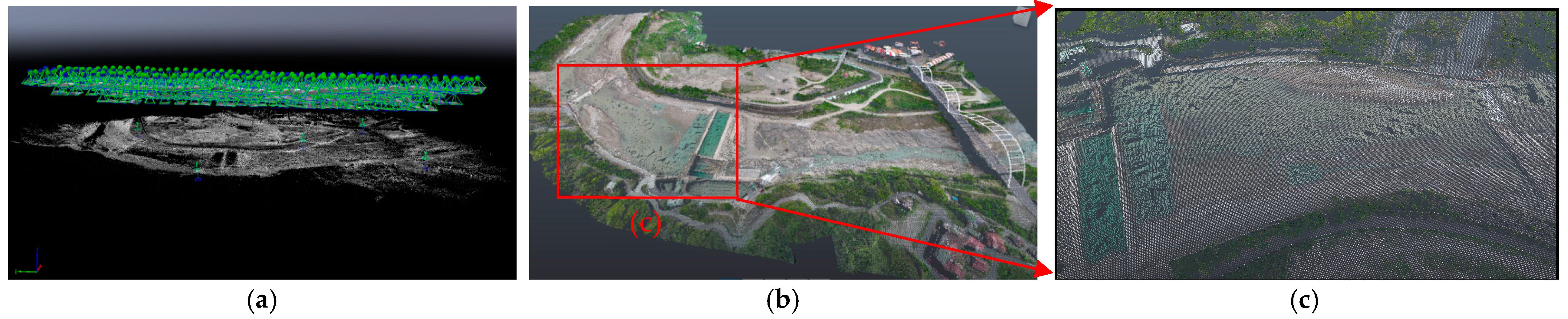
Figure 9.
The point cloud generated by Pix4D software. (a) Generated point cloud based on UAV aerial pictures, (b) final point cloud picture, and (c) the zoom-in view of point cloud of the study area.
Figure 9.
The point cloud generated by Pix4D software. (a) Generated point cloud based on UAV aerial pictures, (b) final point cloud picture, and (c) the zoom-in view of point cloud of the study area.

Figure 10.
GEP modeling operation flowchart [36].
Figure 10.
GEP modeling operation flowchart [36].

Figure 11.
Bathymetry retrieval results from GEP and REG models.

Figure 12.
The illustration of the GEP bathymetry retrieval model.

Figure 13.
The absolute error (AE) of modeled and observed water depth of the testing dataset.

Figure 14.
Frequency distribution of water depth AE of the testing dataset.


Table 1.
The information from the quality report of each UAV flight missions.
| Items | 6 April 2016 | 10 April 2017 | 2 May 2017 |
|---|---|---|---|
| Images | 772 | 1076 | 856 |
| Median of Key-points per Image | 20,000 | 21,111 | 53,203 |
| Median of Matching Points per Image | 8870.85 | 5889.67 | 12,485.60 |
| Ground Control Points (GCP) | 20 | 19 | 6 |
| The Mean RMS Error of GCP in X-axis | 0.009 m | 0.006 m | 0.003 m |
| The Mean RMS Error of GCP in Y-axis | 0.007 m | 0.004 m | 0.004 m |
| The Mean RMS Error of GCP in Z-axis | 0.013 m | 0.008 m | 0.004 m |
| Number of 3D Densified Points | 97,694,554 | 125,818,685 | 400,257,260 |
| Average Density (per m3) | 37.37 | 64.61 | 776.11 |
Table 2.
Spectral sample data description (n = 171).
| Index | Max | Min | Average | Standard Deviation |
|---|---|---|---|---|
| Green | 0.094 | 0.038 | 0.071 | 0.008 |
| NIR | 0.079 | 0.044 | 0.065 | 0.008 |
| NDVI | 0.148 | −0.323 | −0.163 | 0.071 |
| NDWI | 0.264 | −0.290 | 0.044 | 0.093 |
Table 3.
Significance test between training dataset (n = 138) and testing dataset (n = 33).
| Variable | Average Values of Variables | p-Value | Significant Difference | ||
|---|---|---|---|---|---|
| Raw Dataset | Training | Testing | |||
| Green | 0.071 | 0.070 | 0.072 | 0.411 | - |
| NIR | 0.065 | 0.065 | 0.064 | 0.446 | - |
| NDVI | −0.163 | −0.162 | −0.172 | 0.450 | - |
| NDWI | 0.044 | 0.041 | 0.063 | 0.244 | - |
| Water Depth (m) | 0.646 | 0.633 | 0.701 | 0.386 | - |
Table 4.
Bathymetry retrieval accuracy of GEP and REG models.
| Model | R2 | MAE (m) | ME (m) | RMSE (m) | ||||
|---|---|---|---|---|---|---|---|---|
| Training | Testing | Training | Testing | Training | Testing | Training | Testing | |
| GEP | 0.632 | 0.801 | 0.188 | 0.154 | 0.003 | 0.012 | 0.242 | 0.195 |
| REG | 0.569 | 0.729 | 0.211 | 0.184 | <0.001 | −0.008 | 0.262 | 0.225 |
Table 5.
MAE comparison for three depth ranges in the testing dataset.
| Model | Observed Bathymetry (m) | |||
|---|---|---|---|---|
| <0.4 | 0.4–0.8 | 0.8–1.48 | 0–1.48 | |
| MAE (m) | ||||
| GEP | 0.194 | 0.110 | 0.163 | 0.154 |
| REG | 0.220 | 0.112 | 0.221 | 0.184 |
Table 6.
Comparison of water depth retrieval results between this study and related research.
| Study | Tool | Factor | Value (m) | Range (m) | |
|---|---|---|---|---|---|
| Method | Remote/Contact 1 | ||||
| Kasvi et al. [16] | ADCP 2 | C | MAE | 0.030–0.070 (avg. 0.053) | 0.20–1.50 |
| Kasvi et al. [16] | REG | R | MAE | 0.050–0.170 (avg. 0.112) | 0.00–1.50 |
| This study | ML (GEP) | R | MAE | 0.154 | 0.01–1.53 |
| This study | REG | R | MAE | 0.184 | 0.01–1.53 |
| Kasvi et al. [16] | SfM | R | MAE | 0.180–2.980 (avg. 0.740) | 0.00–1.50 |
| This study | REG | R | ME | −0.008 | 0.01–1.53 |
| This study | ML (GEP) | R | ME | 0.012 | 0.01–1.53 |
| Kasvi et al. [16] | ADCP 2 | C | ME | −0.030–0.000 (avg. −0.015) | 0.20–1.50 |
| Kasvi et al. [16] | REG | R | ME | −0.170–0.020 (avg. −0.087) | 0.00–1.50 |
| Jérôme et al. [21] | REG | R | ME | 0.130 | 0.09–1.01 |
| Mandlburger et al. [39] | ML (DL) | R | ME | 0.150 | 0.00–12.00 |
| Kasvi et al. [16] | SfM | R | ME | −0.180–3.200 (avg. 0.357) | 0.00–1.50 |
| Sagawa et al. [40] | ML (RF) | R | ME | 0.250–1.370 (avg. 1.008) | 0.00–5.00 |
| This study | ML (GEP) | R | RMSE | 0.195 | 0.01–1.53 |
| This study | REG | R | RMSE | 0.225 | 0.01–1.53 |
| Lee et al. [23] | ML (NN) | R | RMSE | 0.310–0.400 (avg. 0.358) | 1.50–9.00 |
| Lee et al. [23] | MBVA | R | RMSE | 0.440 | 1.50–9.00 |
| Sandidge and Holyer [41] | ML (NN) | R | RMSE | 0.480 | 0.00–6.00 |
| Lee et al. [23] | ML (NN) | R | RMSE | 0.510–0.520 (avg. 0.515) | 1.00–11.00 |
| Lee et al. [23] | MBVA | R | RMSE | 0.540 | 1.00–11.00 |
| Lee et al. [23] | TBRA | R | RMSE | 1.020 | 1.50–9.00 |
| Lee et al. [23] | TBRA | R | RMSE | 1.250 | 1.00–11.00 |
| Hernandez and Armstrong [15] | REG | R | RMSE | 1.260 | 1.00–10.00 |
| Su et al. [34] | REG | R | RMSE | 1.340 | 0.00–5.00 |
| Sagawa et al. [40] | ML (RF) | R | RMSE | 0.830–1.910 (avg. 1.634) | 0.00–5.00 |
| Su et al. [34] | ML (LM) | R | RMSE | 2.070 | 0.00–5.00 |
1 R: Remote sensing; C: Contact measurement. 2 The investigation range of ADCP is from 0.2 m to 1.5 m due to the equipment limitation. ADCP: acoustic Doppler current profiler; ML: machine learning; RF: random forest; NN: neural network; LM: Levenberg–Marquardt; DL: deep learning; SfM: specific structure from motion; MBVA: multiband value algorithm; TBRA: two-band ratio algorithm.
Publisher’s Note: MDPI stays neutral with regard to jurisdictional claims in published maps and institutional affiliations. |
© 2022 by the authors. Licensee MDPI, Basel, Switzerland. This article is an open access article distributed under the terms and conditions of the Creative Commons Attribution (CC BY) license (https://creativecommons.org/licenses/by/4.0/).
Share and Cite
MDPI and ACS Style
Lee, C.-H.; Liu, L.-W.; Wang, Y.-M.; Leu, J.-M.; Chen, C.-L. Drone-Based Bathymetry Modeling for Mountainous Shallow Rivers in Taiwan Using Machine Learning. Remote Sens. 2022, 14, 3343. https://0-doi-org.brum.beds.ac.uk/10.3390/rs14143343
AMA Style
Lee C-H, Liu L-W, Wang Y-M, Leu J-M, Chen C-L. Drone-Based Bathymetry Modeling for Mountainous Shallow Rivers in Taiwan Using Machine Learning. Remote Sensing. 2022; 14(14):3343. https://0-doi-org.brum.beds.ac.uk/10.3390/rs14143343
Chicago/Turabian StyleLee, Chih-Hung, Li-Wei Liu, Yu-Min Wang, Jan-Mou Leu, and Chung-Ling Chen. 2022. "Drone-Based Bathymetry Modeling for Mountainous Shallow Rivers in Taiwan Using Machine Learning" Remote Sensing 14, no. 14: 3343. https://0-doi-org.brum.beds.ac.uk/10.3390/rs14143343
Note that from the first issue of 2016, this journal uses article numbers instead of page numbers. See further details here.