
A Rapid Model (COV_PSDI) for Winter Wheat Mapping in Fallow Rotation Area Using MODIS NDVI Time-Series Satellite Observations: The Case of the Heilonggang Region


Abstract
:1. Introduction
2. Materials and Methods
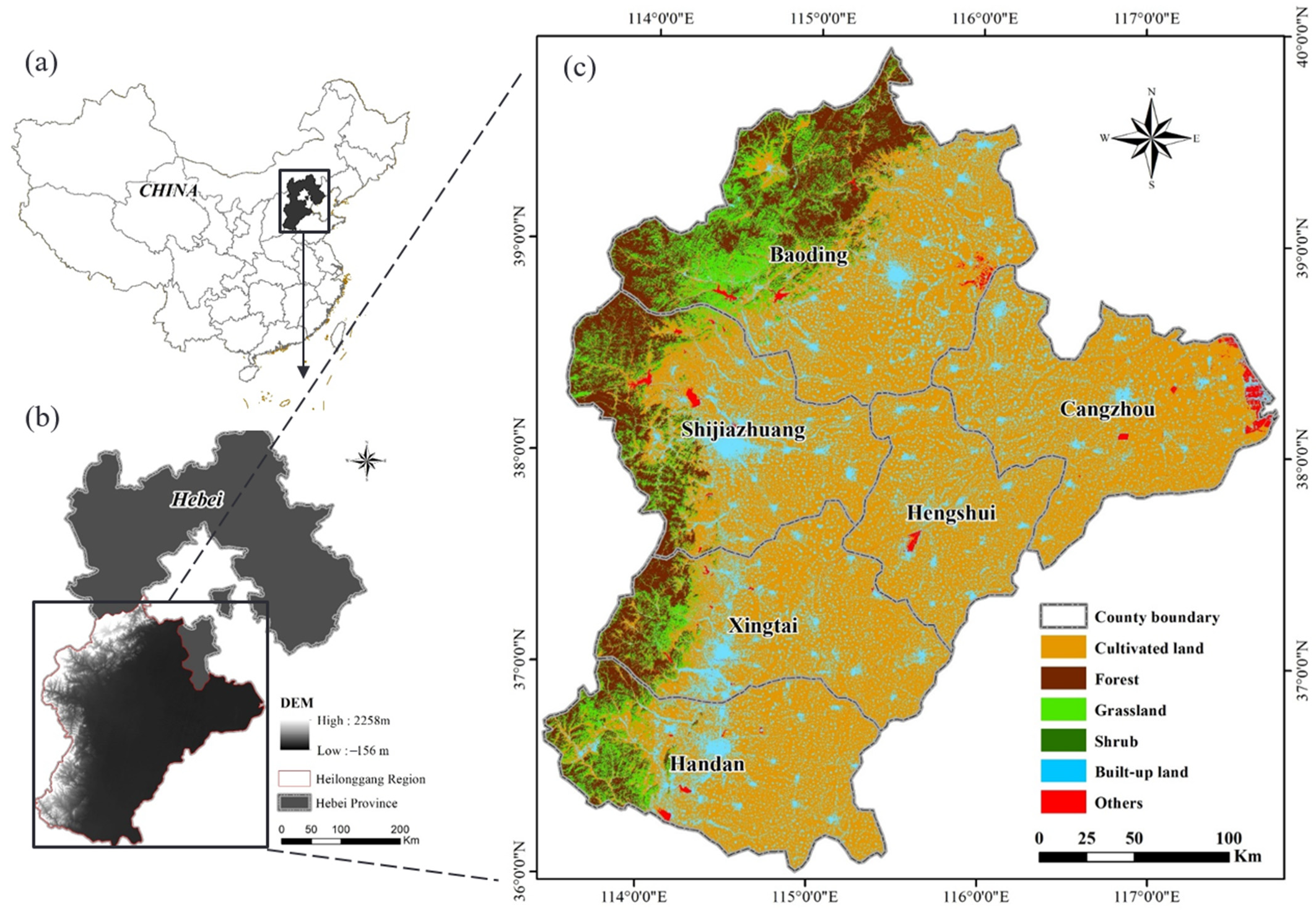
2.1. Study Area
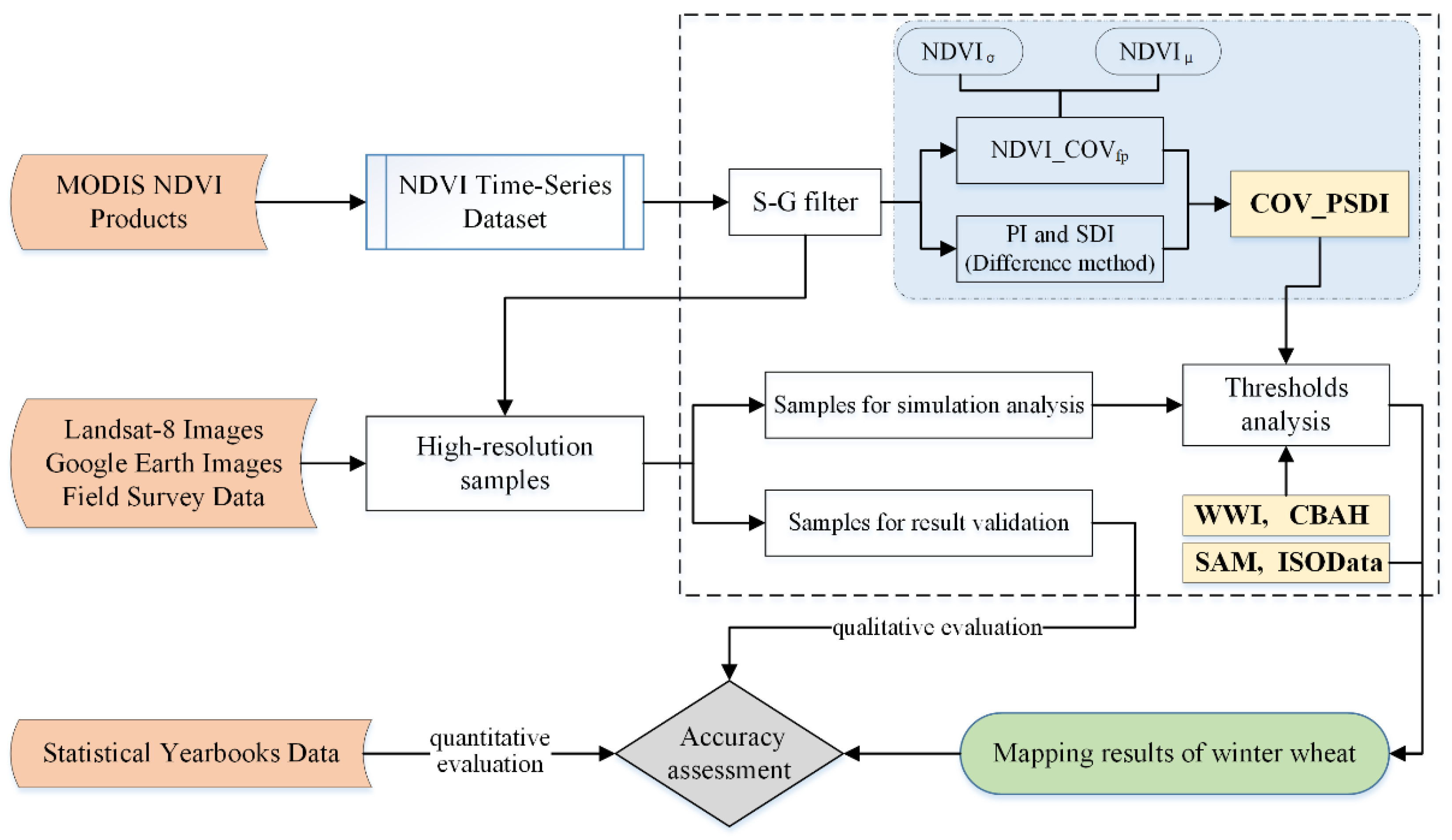
2.2. Workflow
2.3. Data and Data Pre-Processing
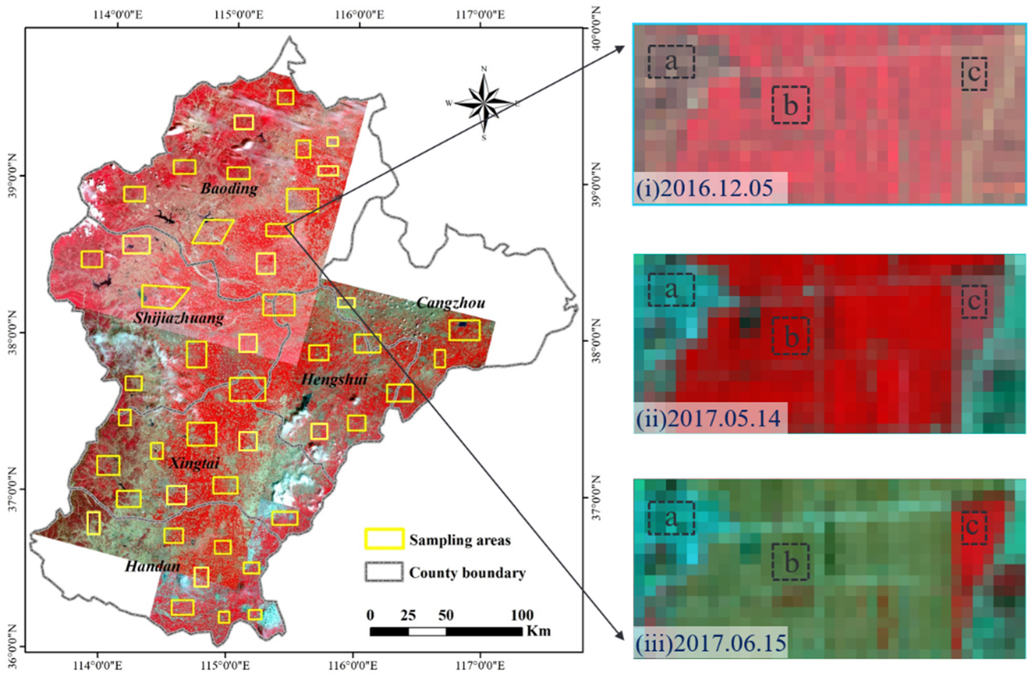
2.3.1. Data
2.3.2. Data Preprocessing
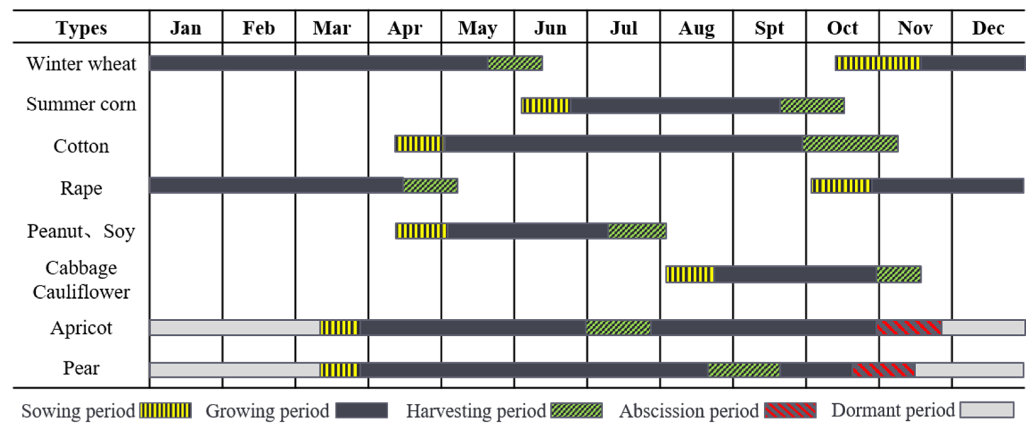
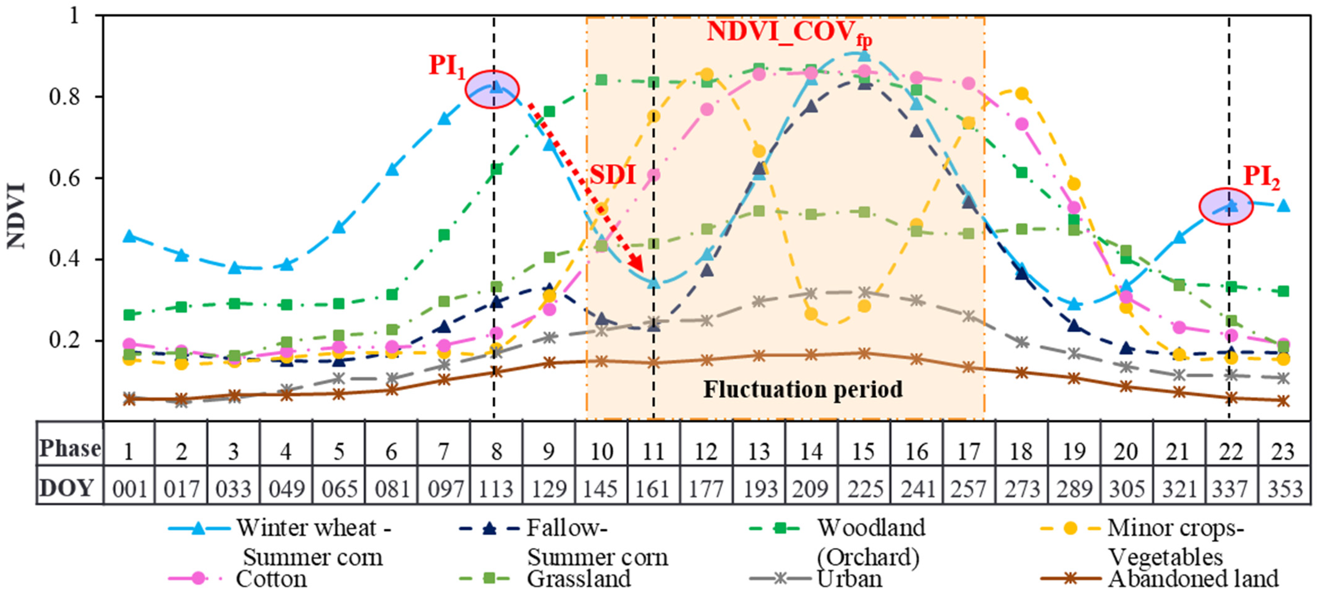
2.4. NDVI Time Series of Different Land Cover Types
2.5. Winter Wheat Extraction Model (COV_PSDI)
2.5.1. Variation Coefficient of Fluctuation Period NDVI_COVfp
2.5.2. Peak and Slope Difference Index PSDI
2.6. Threshold Analysis
2.7. Accuracy Assessment and Model Comparison
3. Results
3.1. Analysis Results of Model Parameters
3.2. Winter Wheat Mapping Results
3.3. Model Comparison and Validation
4. Discussion
5. Conclusions
Author Contributions
Funding
Conflicts of Interest
Abbreviations
| Abbreviation | Description |
| CBAH | combining variations before and after estimated heading dates |
| CLCD | annual China Land Cover Dataset |
| COV | coefficient of variation |
| DOY | the day of a year |
| EVE | early growth stage (seeding stage to heading stage) |
| EVI | enhanced vegetation index |
| EVL | late growth stage (heading stage to harvesting stage) |
| ISODATA | iterative self-organizing data analysis technique algorithm |
| MODIS | Moderate Resolution Imaging Spectroradiometer |
| MRT | MODIS reprojection tool |
| MVC | maximum value composite |
| NASA | National Aeronautics and Space Administration |
| NDVI | normalized difference vegetation index |
| NDVI_COV | variation coefficient of time-series NDVI |
| NDVI_COVannual | annual variation coefficient of NDVI time-series |
| NDVI_COVfp | variation coefficient of time-series NDVI in fluctuation period |
| NIR | near-infrared |
| OA | overall accuracy |
| OLI | operational land imager |
| PA | producer accuracy |
| PE | percentage error |
| PI | peak index |
| PSDI | peak-slope difference index |
| RF | random forests |
| SAM | spectral angle mapping |
| SDI | slope difference index |
| S-G | Savitzky-Golay |
| SVM | support vector machine |
| UA | user accuracy |
| USGS | U.S. Geological Survey |
| WWI | winter wheat index |
References
- Chen, Y.; Zhang, Z.; Tao, F. Improving regional winter wheat yield estimation through assimilation of phenology and leaf area index from remote sensing data. Eur. J. Agron. 2018, 101, 163–173. [Google Scholar] [CrossRef]
- Zhang, D.; Fang, S.; She, B.; Zhang, H.; Jin, N.; Xia, H.; Yang, Y.; Ding, Y. Winter Wheat Mapping Based on Sentinel-2 Data in Heterogeneous Planting Conditions. Remote Sens. 2019, 11, 2647. [Google Scholar] [CrossRef] [Green Version]
- Zhou, T.; Pan, J.; Zhang, P.; Wei, S.; Han, T. Mapping Winter Wheat with Multi-Temporal SAR and Optical Images in an Urban Agricultural Region. Sensors 2017, 17, 1210. [Google Scholar] [CrossRef] [PubMed]
- Zhang, X.; Qiu, F.; Qin, F. Identification and mapping of winter wheat by integrating temporal change information and Kullback–Leibler divergence. Int. J. Appl. Earth. Obs. 2019, 76, 26–39. [Google Scholar] [CrossRef]
- Tao, J.; Wu, W.; Zhou, Y.; Wang, Y.; Jiang, Y. Mapping winter wheat using phenological feature of peak before winter on the North China Plain based on time-series MODIS data. J. Integr. Agric. 2017, 16, 348–359. [Google Scholar] [CrossRef] [Green Version]
- Wang, J.; Jiang, Y.; Wang, H.; Huang, Q.; Deng, H. Groundwater irrigation and management in northern China: Status, trends, and challenges. Int. J. Water Resour. Dev. 2020, 36, 670–696. [Google Scholar] [CrossRef]
- Wu, X.; Qi, Y.; Shen, Y.; Yang, W.; Zhang, Y.; Kondoh, A. Change of winter wheat planting area and its impacts on groundwater depletion in the North China Plain. J. Geogr. Sci. 2019, 29, 891–908. [Google Scholar] [CrossRef] [Green Version]
- Li, Q.; Ma, L.Y.; Wang, X.F.; Wei, M.; Shi, Q.H.; Yang, F.J. Effects of short-term summer fallow and rotations on soil quality under plastic greenhouse cultivation. J. Food Agric. Environ. 2012, 10, 1106–1110. [Google Scholar]
- Yang, X.; Steenhuis, T.; Davis, K.; Van der Werf, W.; Ritsema, C.; Pacenka, S.; Zhang, F.; Siddique, K.; Du, T. Diversified crop rotations enhance groundwater and economic sustainability of food production. Food. Energy Secur. 2021, 10, e311. [Google Scholar] [CrossRef]
- Skakun, S.; Franch, B.; Vermote, E.; Roger, J.-C.; Becker-Reshef, I.; Justice, C.; Kussul, N. Early season large-area winter crop mapping using MODIS NDVI data, growing degree days information and a Gaussian mixture model. Remote Sens. Environ. 2017, 195, 244–258. [Google Scholar] [CrossRef]
- Wu, D.; Yu, Q.; Lu, C.; Hengsdijk, H. Quantifying production potentials of winter wheat in the North China Plain. Eur. J. Agron. 2006, 24, 226–235. [Google Scholar] [CrossRef]
- Khan, A.; Hansen, M.C.; Potapov, P.V.; Adusei, B.; Pickens, A.; Krylov, A.; Stehman, S.V. Evaluating Landsat and RapidEye Data for Winter Wheat Mapping and Area Estimation in Punjab, Pakistan. Remote Sens. 2018, 10, 489. [Google Scholar] [CrossRef] [Green Version]
- Liu, J.; Zhu, W.; Atzberger, C.; Zhao, A.; Pan, Y.; Huang, X. A Phenology-Based Method to Map Cropping Patterns under a Wheat-Maize Rotation Using Remotely Sensed Time-Series Data. Remote Sens. 2018, 10, 1203. [Google Scholar] [CrossRef] [Green Version]
- Wu, M.; Huang, W.; Niu, Z.; Wang, Y.; Wang, C.; Li, W.; Hao, P.; Yu, B. Fine crop mapping by combining high spectral and high spatial resolution remote sensing data in complex heterogeneous areas. Comput. Electron. Agric. 2017, 139, 1–9. [Google Scholar] [CrossRef]
- Li, X.; Wu, T.; Liu, K.; Li, Y.; Zhang, L. Evaluation of the Chinese Fine Spatial Resolution Hyperspectral Satellite TianGong-1 in Urban Land-Cover Classification. Remote Sens. 2016, 8, 438. [Google Scholar] [CrossRef] [Green Version]
- Gilbertson, J.K.; Kemp, J.; van Niekerk, A. Effect of pan-sharpening multi-temporal Landsat 8 imagery for crop type differentiation using different classification techniques. Comput. Electron. Agric. 2017, 134, 151–159. [Google Scholar] [CrossRef] [Green Version]
- Jin, N.; Tao, B.; Ren, W.; Feng, M.; Sun, R.; He, L.; Zhuang, W.; Yu, Q. Mapping Irrigated and Rainfed Wheat Areas Using Multi-Temporal Satellite Data. Remote Sens. 2016, 8, 207. [Google Scholar] [CrossRef] [Green Version]
- Qin, Y.; Xiao, X.; Dong, J.; Zhou, Y.; Zhu, Z.; Zhang, G.; Du, G.; Jin, C.; Kou, W.; Wang, J.; et al. Mapping paddy rice planting area in cold temperate climate region through analysis of time series Landsat 8 (OLI), Landsat 7 (ETM+) and MODIS imagery. ISPRS J. Photogramm. 2015, 105, 220–233. [Google Scholar] [CrossRef] [Green Version]
- Fang, H.; Wei, Y.; Dai, Q. A Novel Remote Sensing Index for Extracting Impervious Surface Distribution from Landsat 8 OLI Imagery. Appl. Sci. 2019, 9, 2631. [Google Scholar] [CrossRef] [Green Version]
- Zheng, B.; Myint, S.W.; Thenkabail, P.S.; Aggarwal, R.M. A support vector machine to identify irrigated crop types using time-series Landsat NDVI data. Int. J. Appl. Earth Obs. 2015, 34, 103–112. [Google Scholar] [CrossRef]
- Zhong, L.; Gong, P.; Biging, G.S. Efficient corn and soybean mapping with temporal extendability: A multi-year experiment using Landsat imagery. Remote Sens. Environ. 2014, 140, 1–13. [Google Scholar] [CrossRef]
- Tian, H.; Huang, N.; Niu, Z.; Qin, Y.; Pei, J.; Wang, J. Mapping Winter Crops in China with Multi-Source Satellite Imagery and Phenology-Based Algorithm. Remote Sens. 2019, 11, 820. [Google Scholar] [CrossRef] [Green Version]
- Martínez-Casasnovas, J.A.; Martín-Montero, A.; Auxiliadora Casterad, M. Mapping multi-year cropping patterns in small irrigation districts from time-series analysis of Landsat TM images. Eur. J. Agron. 2005, 23, 159–169. [Google Scholar] [CrossRef]
- Castillejo-González, I.L.; López-Granados, F.; García-Ferrer, A.; Peña-Barragán, J.M.; Jurado-Expósito, M.; de la Orden, M.S.; González-Audicana, M. Object- and pixel-based analysis for mapping crops and their agro-environmental associated measures using QuickBird imagery. Comput. Electron. Agric. 2009, 68, 207–215. [Google Scholar] [CrossRef]
- Conese, C.; Maselli, F. Use of multitemporal information to improve classification performance of TM scenes in complex terrain. ISPRS J. Photogramm. 1991, 46, 187–197. [Google Scholar] [CrossRef]
- Whitcraft, A.K.; Vermote, E.F.; Becker-Reshef, I.; Justice, C.O. Cloud cover throughout the agricultural growing season: Impacts on passive optical earth observations. Remote Sens. Environ. 2015, 156, 438–447. [Google Scholar] [CrossRef]
- Liu, K.; Su, H.; Zhang, L.; Yang, H.; Zhang, R.; Li, X. Analysis of the Urban Heat Island Effect in Shijiazhuang, China Using Satellite and Airborne Data. Remote Sens. 2015, 7, 4804. [Google Scholar] [CrossRef] [Green Version]
- Li, X.; Liu, K.; Tian, J. Variability, predictability, and uncertainty in global aerosols inferred from gap-filled satellite observations and an econometric modeling approach. Remote Sens. Environ. 2021, 261, 112501. [Google Scholar] [CrossRef]
- Wardlow, B.D.; Egbert, S.L.; Kastens, J.H. Analysis of time-series MODIS 250 m vegetation index data for crop classification in the U.S. Central Great Plains. Remote Sens. Environ. 2007, 108, 290–310. [Google Scholar] [CrossRef] [Green Version]
- Becker-Reshef, I.; Vermote, E.; Lindeman, M.; Justice, C. A generalized regression-based model for forecasting winter wheat yields in Kansas and Ukraine using MODIS data. Remote Sens. Environ. 2010, 114, 1312–1323. [Google Scholar] [CrossRef]
- Pan, Y.; Li, L.; Zhang, J.; Liang, S.; Zhu, X.; Sulla-Menashe, D. Winter wheat area estimation from MODIS-EVI time series data using the Crop Proportion Phenology Index. Remote Sens. Environ. 2012, 119, 232–242. [Google Scholar] [CrossRef]
- Dong, J.; Fu, Y.; Wang, J.; Tian, H.; Fu, S.; Niu, Z.; Han, W.; Zheng, Y.; Huang, J.; Yuan, W. Early-season mapping of winter wheat in China based on Landsat and Sentinel images. Earth Syst. Sci. Data. 2020, 12, 3081–3095. [Google Scholar] [CrossRef]
- Qu, C.; Li, P.; Zhang, C. A spectral index for winter wheat mapping using multi-temporal Landsat NDVI data of key growth stages. ISPRS J. Photogramm. 2021, 175, 431–447. [Google Scholar] [CrossRef]
- Sarvia, F.; Xausa, E.; De Petris, S.; Cantamessa, G.; Borgogno-Mondino, E. A Possible Role of Copernicus Sentinel-2 Data to Support Common Agricultural Policy Controls in Agriculture. Agronomy 2021, 11, 110. [Google Scholar] [CrossRef]
- Chu, L.; Liu, Q.; Huang, C.; Liu, G. Monitoring of winter wheat distribution and phenological phases based on MODIS time-series: A case study in the Yellow River Delta, China. J. Integr. Agric. 2016, 15, 2403–2416. [Google Scholar] [CrossRef]
- Qiu, B.; Luo, Y.; Tang, Z.; Chen, C.; Lu, D.; Huang, H.; Chen, Y.; Chen, N.; Xu, W. Winter wheat mapping combining variations before and after estimated heading dates. ISPRS J. Photogramm. 2017, 123, 35–46. [Google Scholar] [CrossRef]
- Jin, M.; Zhang, R.; Sun, L.; Gao, Y. Temporal and spatial soil water management: A case study in the Heilonggang region, PR China. Agric. Water Manag. 1999, 42, 173–187. [Google Scholar] [CrossRef]
- He, J.; Li, H.; Rasaily, R.G.; Wang, Q.; Cai, G.; Su, Y.; Qiao, X.; Liu, L. Soil properties and crop yields after 11 years of no tillage farming in wheat–maize cropping system in North China Plain. Soil Tillage Res. 2011, 113, 48–54. [Google Scholar] [CrossRef]
- Jia, K.; Wu, B.; Li, Q. Crop classification using HJ satellite multispectral data in the North China Plain. J. Appl. Remote Sens. 2013, 3576, 073576. [Google Scholar] [CrossRef]
- Jingsong, S.; Guangsheng, Z.; Xinghua, S. Climatic suitability of the distribution of the winter wheat cultivation zone in China. Eur. J. Agron. 2012, 43, 77–86. [Google Scholar] [CrossRef]
- Kang, S.; Eltahir, E.A.B. North China Plain threatened by deadly heatwaves due to climate change and irrigation. Nat Commun 2018, 9, 2894. [Google Scholar] [CrossRef] [PubMed] [Green Version]
- Wang, X.; Li, X.; Xin, L. Impact of the shrinking winter wheat sown area on agricultural water consumption in the Hebei Plain. J. Geogr. Sci. 2014, 24, 313–330. [Google Scholar] [CrossRef]
- Wu, Z.; Thenkabail, P.; Mueller, R.; Zakzeski, A.; Melton, F.; Johnson, L.; Rosevelt, C.; Dwyer, J.; Jones, J.; Verdin, J. Seasonal cultivated and fallow cropland mapping using MODIS-based automated cropland classification algorithm. J. Appl. Remote Sens. 2014, 8, 083685. [Google Scholar] [CrossRef] [Green Version]
- Chen, Y.; Lu, D.; Moran, E.; Batistella, M.; Dutra, L.V.; Sanches, I.D.A.; da Silva, R.F.B.; Huang, J.; Luiz, A.J.B.; de Oliveira, M.A.F. Mapping croplands, cropping patterns, and crop types using MODIS time-series data. Int. J. Appl. Earth Obs. 2018, 69, 133–147. [Google Scholar] [CrossRef]
- Wardlow, B.D.; Egbert, S.L. A comparison of MODIS 250-m EVI and NDVI data for crop mapping: A case study for southwest Kansas. Int. J. Remote Sens. 2010, 31, 805–830. [Google Scholar] [CrossRef]
- Onojeghuo, A.; Blackburn, G.; Wang, Q.; Atkinson, P.; Kindred, D.; Miao, Y. Rice crop phenology mapping at high spatial and temporal resolution using downscaled MODIS time-series. GISci. Remote Sens. 2018, 55, 659–677. [Google Scholar] [CrossRef] [Green Version]
- Yang, J.; Huang, X. The 30 m annual land cover dataset and its dynamics in China from 1990 to 2019. Earth Syst. Sci. Data 2021, 13, 3907–3925. [Google Scholar] [CrossRef]
- Savitzky, A.; Golay, M.J.E. Smoothing and Differentiation of Data by Simplified Least Squares Procedures. Anal. Chem. 1964, 36, 1627–1639. [Google Scholar] [CrossRef]
- Chen, J.; Jönsson, P.; Tamura, M.; Gu, Z.; Matsushita, B.; Eklundh, L. A simple method for reconstructing a high-quality NDVI time-series data set based on the Savitzky–Golay filter. Remote Sens. Environ. 2004, 91, 332–344. [Google Scholar] [CrossRef]
- Wardlow, B.D.; Egbert, S.L. Large-area crop mapping using time-series MODIS 250 m NDVI data: An assessment for the U.S. Central Great Plains. Remote Sens. Environ. 2008, 112, 1096–1116. [Google Scholar] [CrossRef]
- Pan, Z.; Huang, J.; Zhou, Q.; Wang, L.; Cheng, Y.; Zhang, H.; Blackburn, G.A.; Yan, J.; Liu, J. Mapping crop phenology using NDVI time-series derived from HJ-1 A/B data. Int. J. Appl. Earth Obs. 2015, 34, 188–197. [Google Scholar] [CrossRef] [Green Version]
- Jonsson, P.; Eklundh, L. Seasonality extraction by function fitting to time-series of satellite sensor data. IEEE Trans. Geosci. Remote. Sens. 2002, 40, 1824–1832. [Google Scholar] [CrossRef]
- Leprieur, C.; Verstraete, M.M.; Pinty, B. Evaluation of the performance of various vegetation indices to retrieve vegetation cover from AVHRR data. Remote Sens. Rev. 1994, 10, 265–284. [Google Scholar] [CrossRef]
- Dong, C.; Zhao, G.; Qin, Y.; Wan, H. Area extraction and spatiotemporal characteristics of winter wheat-summer maize in Shandong Province using NDVI time series. PLoS ONE 2019, 14, e0226508. [Google Scholar] [CrossRef] [PubMed] [Green Version]
- Yang, Y.; Wu, T.; Wang, S.; Li, J.; Muhanmmad, F. The NDVI-CV Method for Mapping Evergreen Trees in Complex Urban Areas Using Reconstructed Landsat 8 Time-Series Data. Forests 2019, 10, 139. [Google Scholar] [CrossRef] [Green Version]
- Weiss, E.; Marsh, S.; Pfirman, E. Application of NOAA-AVHRR NDVI time-series data to assess changes in Saudi Arabia’s rangelands. Int. J. Remote. Sens. 2001, 22, 1005–1027. [Google Scholar] [CrossRef]
- Fan, J.; Wu, B. A methodology for retrieving cropping index from NDVI profile. J. Remote Sens. 2004, 8, 628–636. [Google Scholar]
- Maxwell, S.K.; Sylvester, K.M. Identification of “ever-cropped” land (1984–2010) using Landsat annual maximum NDVI image composites: Southwestern Kansas case study. Remote Sens. Environ. 2012, 121, 186–195. [Google Scholar] [CrossRef] [Green Version]
- Goldblatt, R.; Stuhlmacher, M.F.; Tellman, B.; Clinton, N.; Hanson, G.; Georgescu, M.; Wang, C.; Serrano-Candela, F.; Khandelwal, A.K.; Cheng, W.-H.; et al. Using Landsat and nighttime lights for supervised pixel-based image classification of urban land cover. Remote Sens. Environ. 2018, 205, 253–275. [Google Scholar] [CrossRef]
- Janssen, L.L.F.; Vanderwel, F.J.M. Accuracy assessment of satellite derived land-cover data: A review. Photogramm. Eng. Remote Sens. 1994, 60, 419–426. [Google Scholar]
- Lu, S.; Deng, R.; Liang, Y.; Xiong, L.; Ai, X.; Qin, Y. Remote Sensing Retrieval of Total Phosphorus in the Pearl River Channels Based on the GF-1 Remote Sensing Data. Remote Sens. 2020, 12, 1420. [Google Scholar] [CrossRef]
- Akinyemi, F.O.; Pontius, R.G.; Braimoh, A.K. Land change dynamics: Insights from Intensity Analysis applied to an African emerging city. J. Spat. Sci. 2017, 62, 69–83. [Google Scholar] [CrossRef]
- Foody, G.M. Explaining the unsuitability of the kappa coefficient in the assessment and comparison of the accuracy of thematic maps obtained by image classification. Remote Sens. Environ. 2020, 239, 111630. [Google Scholar] [CrossRef]
- Pontius, R.G. Component intensities to relate difference by category with difference overall. Int. J. Appl. Earth Obs. 2019, 77, 94–99. [Google Scholar] [CrossRef]
- Pontius, R.G.; Millones, M. Death to Kappa: Birth of quantity disagreement and allocation disagreement for accuracy assessment. Int. J. Remote Sens. 2011, 32, 4407–4429. [Google Scholar] [CrossRef]
- Singh, A. Review Article Digital change detection techniques using remotely-sensed data. Int. J. Remote Sens. 1989, 10, 989–1003. [Google Scholar] [CrossRef] [Green Version]
- Liu, Y.; Lu, S.; Lu, X.; Wang, Z.; Chen, C.; He, H. Classification of Urban Hyperspectral Remote Sensing Imagery Based on Optimized Spectral Angle Mapping. J. Indian Soc. Remote. 2019, 47, 289–294. [Google Scholar] [CrossRef]
- Melesse, A.; Jordan, J. A comparison of fuzzy vs. augmented-ISODATA classification algorithms for cloud-shadow discrimination from Landsat images. Photogramm. Eng. Remote Sens. 2002, 68, 905–911. [Google Scholar] [CrossRef]
- Qiu, S.; Zhu, Z.; He, B. Fmask 4.0: Improved cloud and cloud shadow detection in Landsats 4–8 and Sentinel-2 imagery. Remote Sens. Environ. 2019, 231, 111205. [Google Scholar] [CrossRef]
- Hunter, E.L.; Power, C.H. An assessment of two classification methods for mapping Thames Estuary intertidal habitats using CASI data. Int. J. Remote Sens. 2002, 23, 2989–3008. [Google Scholar] [CrossRef]
- Shahriar Pervez, M.; Budde, M.; Rowland, J. Mapping irrigated areas in Afghanistan over the past decade using MODIS NDVI. Remote Sens. Environ. 2014, 149, 155–165. [Google Scholar] [CrossRef] [Green Version]
- Ahmad, A.; Sufahani, S.F. Analysis of Landsat 5 TM data of Malaysian land covers using ISODATA clustering technique. In Proceedings of the 2012 IEEE Asia-Pacific Conference on Applied Electromagnetics (APACE), Melaka, Malaysia, 11–13 December 2012; pp. 92–97. [Google Scholar] [CrossRef] [Green Version]
- Li, J.; Lei, H. Tracking the spatio-temporal change of planting area of winter wheat-summer maize cropping system in the North China Plain during 2001–2018. Comput. Electron. Agric. 2021, 187, 106222. [Google Scholar] [CrossRef]
- Xie, H.; Cheng, L.; Lv, T. Factors Influencing Farmer Willingness to Fallow Winter Wheat and Ecological Compensation Standards in a Groundwater Funnel Area in Hengshui, Hebei Province, China. Sustainability 2017, 9, 839. [Google Scholar] [CrossRef] [Green Version]
- Ju, J.; Masek, J.G. The vegetation greenness trend in Canada and US Alaska from 1984–2012 Landsat data. Remote Sens. Environ. 2016, 176, 1–16. [Google Scholar] [CrossRef]
- Sakamoto, T.; Yokozawa, M.; Toritani, H.; Shibayama, M.; Ishitsuka, N.; Ohno, H. A crop phenology detection method using time-series MODIS data. Remote Sens. Environ. 2005, 96, 366–374. [Google Scholar] [CrossRef]
- Li, F.; Ren, J.; Wu, S.; Zhao, H.; Zhang, N. Comparison of Regional Winter Wheat Mapping Results from Different Similarity Measurement Indicators of NDVI Time Series and Their Optimized Thresholds. Remote Sens. 2021, 13, 1162. [Google Scholar] [CrossRef]
- Zhang, X.; Zhang, M.; Zheng, Y.; Wu, B. Crop Mapping Using PROBA-V Time Series Data at the Yucheng and Hongxing Farm in China. Remote Sens. 2016, 8, 915. [Google Scholar] [CrossRef] [Green Version]
- Junges, A.; Fontana, D.; Pinto, D. Identification of croplands of winter cereals in Rio Grande do Sul state, Brazil, through unsupervised classification of normalized difference vegetation index images. Eng. Agrícola 2013, 33, 883–895. [Google Scholar] [CrossRef] [Green Version]
- Kar, S.; Rathore, V.S.; Champati Ray, P.K.; Sharma, R.; Swain, S.K. Classification of river water pollution using Hyperion data. J. Hydrol. 2016, 537, 221–233. [Google Scholar] [CrossRef]
- Nguyen, L.H.; Joshi, D.R.; Clay, D.E.; Henebry, G.M. Characterizing land cover/land use from multiple years of Landsat and MODIS time series: A novel approach using land surface phenology modeling and random forest classifier. Remote Sens. Environ. 2020, 238, 111017. [Google Scholar] [CrossRef]
- Wang, L.; Qi, F.; Shen, X.; Huang, J. Monitoring Multiple Cropping Index of Henan Province, China Based on MODIS-EVI Time Series Data and Savitzky-Golay Filtering Algorithm. Comput. Modeling Eng. Sci. 2019, 119, 331–348. [Google Scholar] [CrossRef] [Green Version]
- Yang, J.; Guo, N.; Huang, L.; Jia, J. Ananlyses on MODIS-NDVI Index Saturation in Northwest China. Plateau Meteorol. 2008, 27, 896–903. [Google Scholar]
- Faramarzi, M.; Heidarizadi, Z.; Mohamadi, A.; Heydari, M. Detection of vegetation cover changes using normalized difference vegetation index in semi-arid rangeland in western Iran. J. Agric. Sci. Technol. 2017, 20, 51–60. [Google Scholar]
- Chaves, M.E.D.; Picoli, M.C.A.; Sanches, I.D. Recent Applications of Landsat 8/OLI and Sentinel-2/MSI for Land Use and Land Cover Mapping: A Systematic Review. Remote Sens. 2020, 12, 3062. [Google Scholar] [CrossRef]
- Pastick, N.J.; Wylie, B.K.; Wu, Z. Spatiotemporal Analysis of Landsat-8 and Sentinel-2 Data to Support Monitoring of Dryland Ecosystems. Remote Sens. 2018, 10, 791. [Google Scholar] [CrossRef] [Green Version]
- Zeng, L.; Wardlow, B.D.; Xiang, D.; Hu, S.; Li, D. A review of vegetation phenological metrics extraction using time-series, multispectral satellite data. Remote Sens. Environ. 2020, 237, 111511. [Google Scholar] [CrossRef]
- Pastick, N.J.; Dahal, D.; Wylie, B.K.; Parajuli, S.; Boyte, S.P.; Wu, Z. Characterizing Land Surface Phenology and Exotic Annual Grasses in Dryland Ecosystems Using Landsat and Sentinel-2 Data in Harmony. Remote Sens. 2020, 12, 725. [Google Scholar] [CrossRef] [Green Version]


| Satellite Data | Acquisition Time | Path/Row | Spatial Resolution | Spectral Resolution | Product Grade | Source |
|---|---|---|---|---|---|---|
| MODIS 1 (384 images) | 1 November 2013–19 December 2017 | h26v04 h26v05 h27v04 h27v05 | 250 m | NDVI | MOD13Q1 | https://ladsweb.modaps.eosdis.nasa.gov/ (accessed on 25 April 2020) |
| Landsat-8 (12 images) | 15 June 2017 | 124/033 | 30 m | Green: (μm) (0.525–0.600) | OLI 3 Reflectance | http://earthexplorer.usgs.gov/ (accessed on 10 April 2020) |
| 14 May 2017 | ||||||
| 5 December 2016 | ||||||
| 15 June 2017 | 124/034 | Red: (μm) (0.630–0.680) | ||||
| 28 April 2017 | ||||||
| 22 January 2017 | ||||||
| 8 June 2017 | 123/034 123/035 | NIR 2: (μm) (0.845–0.885) | ||||
| 7 May 2017 | ||||||
| 14 December 2016 | ||||||
| CLCD 4 [47] | 2017 | 30 m | Land Cover | Version 1.0.0 | https://0-doi-org.brum.beds.ac.uk/10.5281/zenodo.4417810 (accessed on 10 March 2021) |
| Model | Equation | Reference |
|---|---|---|
| CBAH 1 | EVI2max1 is the maximum EVI value in the heading stage; EVI2min1 and EVI2min2 is the minimum EVI value in the seeding and harvesting stage, respectively. | Qiu et al. [36] |
| WWI 4 | NDVImax1 and NDVImax2 are the maximum NDVI value in the over-wintering stage and heading stage, respectively; NDVImin1 and NDVImin2 are the minimum NDVI value in the seeding stage and harvesting stage, respectively. | Qu et al. [33] |
| Models | Identification | Verification | UA | |
|---|---|---|---|---|
| Winter Wheat | Non-Winter Wheat | |||
| COV_PSDI | Winter wheat | 464 | 31 | 93.74% |
| Non-winter wheat | 28 | 477 | ||
| PA | 94.32% | |||
| OA | 94.10% | |||
| SAM | Winter wheat | 451 | 52 | 89.66% |
| Non-winter wheat | 41 | 456 | ||
| PA | 91.67% | |||
| OA | 90.70% | |||
| ISOData | Winter wheat | 457 | 88 | 83.85% |
| Non-winter wheat | 35 | 420 | ||
| PA | 92.89% | |||
| OA | 87.70% | |||
| CBAH | Winter wheat | 461 | 61 | 88.31% |
| Non-winter wheat | 31 | 447 | ||
| PA | 93.70% | |||
| OA | 90.80% | |||
| WWI | Winter wheat | 489 | 107 | 82.05% |
| Non-winter wheat | 3 | 401 | ||
| PA | 99.39% | |||
| OA | 89.00% | |||
| Year | Statistical Data (km2) | COV_PSDI | SAM | ISOData | CBAH | WWI | |||||
|---|---|---|---|---|---|---|---|---|---|---|---|
| Extracted Area (km2) | PE (%) | Extracted Area (km2) | PE (%) | Extracted Area (km2) | PE (%) | Extracted Area (km2) | PE (%) | Extracted Area (km2) | PE (%) | ||
| 2014 | 21,615.0 | 22,076.2 | 2.1 | 20,776.7 | 3.9 | 27,375.3 | 26.6 | 20,961.3 | 3.0 | 23,123.0 | 7.0 |
| 2015 | 21,297.2 | 22,072.8 | 3.6 | 22,718.7 | 6.7 | 29,249.9 | 37.3 | 15,938.4 | 25.2 | 24,525.6 | 15.2 |
| 2016 | 20,739.7 | 20,416.8 | 1.6 | 22,272.7 | 7.4 | 21,640.6 | 4.3 | 16,243.9 | 21.7 | 24,954.6 | 20.3 |
| 2017 | 22,062.8 | 22,821.3 | 3.4 | 24,469.8 | 10.9 | 26,944.9 | 22.1 | 24,681.9 | 11.9 | 23,875.3 | 8.2 |
Publisher’s Note: MDPI stays neutral with regard to jurisdictional claims in published maps and institutional affiliations. |
© 2021 by the authors. Licensee MDPI, Basel, Switzerland. This article is an open access article distributed under the terms and conditions of the Creative Commons Attribution (CC BY) license (https://creativecommons.org/licenses/by/4.0/).
Share and Cite
Zhang, X.; Liu, K.; Wang, S.; Long, X.; Li, X. A Rapid Model (COV_PSDI) for Winter Wheat Mapping in Fallow Rotation Area Using MODIS NDVI Time-Series Satellite Observations: The Case of the Heilonggang Region. Remote Sens. 2021, 13, 4870. https://0-doi-org.brum.beds.ac.uk/10.3390/rs13234870
Zhang X, Liu K, Wang S, Long X, Li X. A Rapid Model (COV_PSDI) for Winter Wheat Mapping in Fallow Rotation Area Using MODIS NDVI Time-Series Satellite Observations: The Case of the Heilonggang Region. Remote Sensing. 2021; 13(23):4870. https://0-doi-org.brum.beds.ac.uk/10.3390/rs13234870
Chicago/Turabian StyleZhang, Xiaoyuan, Kai Liu, Shudong Wang, Xin Long, and Xueke Li. 2021. "A Rapid Model (COV_PSDI) for Winter Wheat Mapping in Fallow Rotation Area Using MODIS NDVI Time-Series Satellite Observations: The Case of the Heilonggang Region" Remote Sensing 13, no. 23: 4870. https://0-doi-org.brum.beds.ac.uk/10.3390/rs13234870