
A New Methodology for the Detection and Extraction of Hyperbolas in GPR Images


Department of Imagery Intelligence, Faculty of Civil Engineering and Geodesy, Military University of Technology (WAT), 00-908 Warsaw, Poland
*
Author to whom correspondence should be addressed.
Remote Sens. 2021, 13(23), 4892; https://0-doi-org.brum.beds.ac.uk/10.3390/rs13234892
Submission received: 7 November 2021
/
Revised: 25 November 2021
/
Accepted: 29 November 2021
/
Published: 2 December 2021
(This article belongs to the Special Issue Latest Results on GPR Algorithms, Applications and Systems)
Abstract
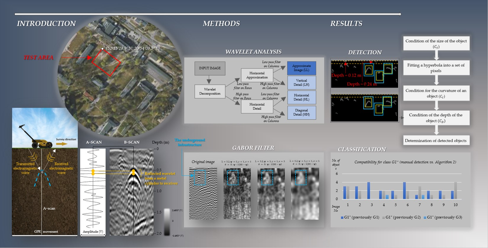
:Reliable detection of underground infrastructure is essential for infrastructure modernization works, the implementation of BIM technology, and 3D cadasters. This requires shortening the time of data interpretation and the automation of the stage of selecting the objects. The main factor that influences the quality of radargrams is noise. The paper presents the method of data filtration with use of wavelet analyses and Gabor filtration. The authors were inspired to conduct the research by the fact that the interpretation and analysis of radargrams is time-consuming and by the wish to improve the accuracy of selection of the true objects by inexperienced operators. The authors proposed automated methods for the detection and classification of hyperboles in GPR images, which include the data filtration, detection, and classification of objects. The proposed object classification methodology based on the analytic hierarchy process method introduces a classification coefficient that takes into account the weights of the proposed conditions and weights of the coefficients. The effectiveness and quality of detection and classification of objects in radargrams were assessed. The proposed methods make it possible to shorten the time of the detection of objects. The developed hyperbola classification coefficients show promising results of the detection and classification of objects.

1. Introduction
The detection of underground objects, in particular utility networks, is widely applied in civil engineering, geodesy, geology, and archaeology. One of the non-invasive geophysical methods for the detection of various underground media is the ground penetrating radar (GPR) method. The operation of such radar is based on the emission of electromagnetic waves that penetrate various geological media, followed by the reception of the beam reflected by the discontinuities of the structure of soil, rock, or material medium [1]. As a result of detection, the device operator obtains a set of radargrams that resemble the cross-section of soil in the given area. Radargrams are two-dimensional images that consist of numerous single signals reflected from soil media and recorded by the receiving antenna. The distance covered by the instrument and the time of recording the return signal may be read from the obtained images. The position of the underground object is defined by the determination of the vertex of the hyperbola. The authors of publication [2] used the curvelet transform that is a development of the wavelet transform for the detection of pipes. What is characteristic for this transform is the possibility to decompose the image with use of the orientation parameter that allows for the interpretation of radargram based on its properties, i.e., edges and shapes. The analysis of coefficients that describe the diagonal details of the image (obtained in the process of its decomposition at a defined level) enabled to partly distinguish the group of the brightest pixels that reflect the actual position of the underground object [2].
In order to interpret the obtained radiograms correctly, they have to be subjected to preliminary processing. This stage involves mainly time-zero correction, removing the background, and the migration and extraction of maximum values [3,4]. The aim of processing radargrams is to improve the efficiency of the interpretation process and ultimately to define the position of buried objects. One of the methods to improve image quality is digital image processing that consists in changing the values of pixels according to specific mathematical rules. This process usually involves the correction of contrast, brightness, sharpening edges, or noise reduction. Another essential element of the analysis of the obtained data is their thorough interpretation and the extraction of characteristic areas. Currently, it is usually conducted with use of two methods, i.e., time and frequency analysis and artificial neural networks [5]. The first of them distinguishes fragments of radargrams with similar frequency characteristics with use of wavelet analyses or Fourier transform [6]. Wavelet analysis is often applied in issues related to denoising of GPR radargrams [7,8]. Although there has been significant progress in time-frequency analyses [9], there is still a need to analyze and select the appropriate tools and methods for the extraction of true objects from images obtained with use of GPR [10].
The issue of distinguishing true objects in radargrams is a research topic of key importance, as interfering hyperbolas that constitute the noise in images hinder the interpretation of true objects. Article [11] demonstrated that only 2% of the data in a GPR image contains useful information. The problem of the detection of interference hyperbolas was analyzed in study [12], whose authors analyzed the application of low pass filters for the reduction of high-frequency noise. The authors of [13] used the innovative multiresolution monogenic signal analysis (MMSA) method, developed by Unser [14], to localize buried objects from GPR images [13]. The components used in this method are a proposal to reduce noise based on wavelet analysis. Buried objects are first distinguished with use of region of interest (ROI) and then detected with Hough transform.
However, most publications on GPR focus on automated detection of hyperbolas. The automation of the process of detecting hyperbolas in GPR images may be applied in particular in the analysis and interpretation of radargrams by inexperienced operators. The authors of study [15] proposed to apply a semi-automated method for the detection of underground objects, which allowed them to shorten the time of image interpretation and analysis by approximately 66%. The obtained probability of detecting a true hyperbola was 80% and of a false object 1%. The method was tested in various locations (over asphalt, grass, and concrete), and its performance was assessed based on the probability of detecting a hyperbola and the object and the estimation of the propagation rate. Authors who analyzed the discussed issues also used artificial neural networks to remove the background that interferes with the position of objects [12,16] and the Viola Jones operator that employs Haar wavelets in calculations. The application of these methods enabled the detection of hyperbolas on the level of 59–76%. The automation of detecting hyperbolas in GPR images may be supported by classically matching the pattern to the objects, Hough transform (a special instance of the Radon transform) [1,13,17,18,19,20,21,22], wavelet [22], and Radon transform [23].
The automated object detection process is preceded by the application of filtration, segmentation, detection of contours of all shapes, image binarization [24], or extrapolation in the proximity of each local maximum [25]. The filtered image may be segmented with use of several techniques, such as area division, edge detection method, area spread, statistics-based segmentation, and the segmentation of adjacent objects. The authors of publication [15] applied gradient operator and thresholding. The value of the [6,12,16,21] threshold was defined in a way that ensures the highest efficiency of the method. On the other hand, study [14] presents the application of the Roberts, Sobel, Previtt, Kirsch, and Scharr operators for the detection of edges in the image. The authors also proposed an method for the detection of horizontal edges, with the aim to reduce the computational load.
The main subject of the present article is the automation of the object detection and classification process in images obtained with use of the GPR method. This issue is closely related to textural analysis which is used in the classification, detection, and segmentation of objects [6]. The aim of textural analysis is to distinguish a specific group of objects characterized by a color, shape, and texture [6].
For changing orientation and frequency parameters, Gabor filters generate a set of filters (so-called bank of filters) characterized by variable properties [26]. The authors of article [27] used Gabor filtration to solve the problem resulting from variable height of antenna and image processing. This stage allowed them to improve the process of the interpretation of radargrams. The issue of textural analysis based on Gabor filters comes down to conducting the process of supervised or unsupervised classification [6].
This article presents the application of methods that support the process of automated detection and classification of objects visible in images obtained with use of ground-penetrating radar. The proposed methods were verified on 12 radargrams obtained regularly (at different times of day and in varying environmental conditions) in a test area, in the form of 5 repeated series (consisting of a total of 60 radargrams).
Research Problem
Most of the authors who conducted research on ground-penetrating radars and radargram analysis discussed, to a certain extent, the issues of automated detection and matching hyperbolas into the set of points obtained from the GPR in order to locate the position of buried objects. A common problem that occurs in radargrams is the large number of hyperbolas, being the reflection of electromagnetic waves from improper objects, such as stones or tree roots [28,29]. Such objects may make it more difficult for an inexperienced operator to select the true hyperbolas that are more than just noise.
The aim of our study is to automate and improve the accuracy of the process of detecting and classifying hyperbolas in GPR images using a proposed classification coefficient and two-stage approach.
What makes our methodology different is the fact that it is just a two-stage process and that radiometric and geometric information is used parallelly. The first stage consists in eliminating erroneous hyperbolas through radiometric analysis of images (Gabor filtration and wavelet analysis) and the preliminary identification of true objects (so called “preliminary objects”). The influence of radiometric and geometric properties on the process of the extraction of hyperbolas was defined. The second stage consists of a more detailed selection of preliminary objects by means of introducing geometrical conditions (conditions for curvature, the size and position in the image, i.e., the depth of installation of area utility networks). The proposed methodology for the classification of objects is based on multi-criteria optimization. Moreover, we developed the classification coefficient Q which automates and supports the process of detecting and identifying underground utility networks by inexperienced operators by means of assigning the hyperbolas detected in the image to classes of significance. Finally, it is the operators who select the hyperbolas in the resulting image or in the original radargram. They also have the possibility to display all sub-stages and to select the hyperbolas that constitute the potential location of underground utility networks.
2. Materials and Methods
Tests were conducted on datasets obtained in Warsaw with the DS2000 ground-penetrating radar manufactured by Leica. Five measurement series were obtained, each of them consisting of 12 profiles (located 5 m from each other) and covering an area of the dimensions of 55 × 85 m. Radargrams were obtained in different seasons in a homogeneous area, which resulted in a dataset for analyzing the repeatability of hyperbolas in images. Each measurement series resulted in obtaining 12 radargrams. Initially, the functioning of the proposed methods was tested on all images, and at the subsequent stages (introduction of conditions), analyses were conducted on 10 images.
2.1. Description of Data Sets
Radargrams were obtained with use of two methods. The first of them used a rectangular grid (of the dimensions of 55 × 85 m) with a base line situated along the surface. In order to assign georeferences to the datasets, we measured the characteristic points of the grid with a GNSS GS15 receiver by Leica. Their coordinates were then recorded in a *.dxf file and imported in the ground-penetrating radar. This stage made it possible to draw the base line in the set of points measured by the receiver. When the second method was used, georeferences were obtained with use of the GNSS module integrated with the GPR, without an independent external antenna.
The set of obtained measurement data consists of 3 measurement series acquired with use of the first method and 2 measurement series obtained with use of the second method.
Measurement parameters were selected in an optimum way that ensures the location of objects that are buried both at small and large depths. Detection was conducted at the depth of approx. 5 m at 100 ns. The ground penetration depth was influenced by the attenuation of electromagnetic waves [2]. The scan interval was approximately 4 cm. The technical parameters according to the technical specifications of the instrument are presented in Table 1.
Depending on the geological medium, the value of its dielectric constant or the so-called relative permittivity (), which is a multiplication of the electric permeability of the medium () to the electric permeability of vacuum (), changes (Equation (1)).
2.2. The Resolution of GPR Measurements
The antenna of a frequency of 700 MHz allows for the detection of objects at very high resolution, but at low depth range. On the other hand, the lower frequency antenna (250 MHz) offers lower resolution, but at the same time, a higher depth range than the 700 MHz antenna. The given frequency carries information about the resolution and depth. The resolution of GPR measurements should be understood as the capacity of instruments to determine the minimum distance, at which two identical targets may be recognized as separate objects. Vertical and horizontal resolution may be distinguished. Their value increases with the increase in the frequency of antennas and the dielectric constant of the medium. The vertical and horizontal resolution of the GPR method may be calculated, respectively, with Equations (2) and (3).
where:
—velocity of propagation of an electromagnetic wave,
—frequency of the antenna,
—vertical resolution capacity of the GPR method,
a—vertical resolution capacity of the GPR method,
—relative dielectric permittivity, and
—reflection limit depth.
Assuming that the analyzed area is dominated by sandy soil with clay and silt, whose relative dielectric permittivity ranges from 11 to 36 and the antenna frequency equals 250 MHz, then the vertical resolution in the GPR method will be 5–9 cm. For the frequency of 700 MHz, the vertical resolution will equal 2–3 cm. The horizontal resolution depends on the reflection limit depth. The value of horizontal resolution decreases with the increase in the depth of the located underground object. For the frequency of 250 MHz, this resolution ranges from 2.2 to 3.3 cm (for = 0.5 m), 3.2–4.3 cm (for = 1 m) to 4.5–6 cm (for = 2 m). The horizontal resolution for the frequency of 700 MHz equals 1.3–1.8 cm (for = 0.5 m), 1.9–2.5 cm (for = 1 m) and 2.7–3.6 cm (for = 2 m).
2.3. Radargram Formation
The present sub-section discusses the issues related to the creation of radargrams and locating the detected buried objects (Section 2.3.1). The obtained images were subjected to pre-processing (Section 2.3.2). The Section 2.3.3 and Section 2.3.4 contains a discussion of the manual selection of candidate objects that reflects the potential location of underground utility networks. In order to verify the situational position (xy) of the points selected manually by the operator, the detection results were confirmed by materials obtained from the National Geodetic and Cartographic Resource—NGCR.
2.3.1. Target Localization
The position of the targets may be determined on the radargram before or after depth correction. Before this correction, the time of recording the signal reflected from the analyzed medium will be displayed on the vertical axis of the radargram. In this case, depth is determined based on the horizontal distance covered by the antenna, the time of recording the signal, the coordinates of the given vertex, and the velocity of signal propagation (Equation (4)). On the other hand, the vertical axis of the corrected image shows the values of depth that are the basis for the direct estimation of the position of underground objects [33].
where:
—the horizontal distance,
—time,
—the propagation speed, and
—the coordinates of the apex.
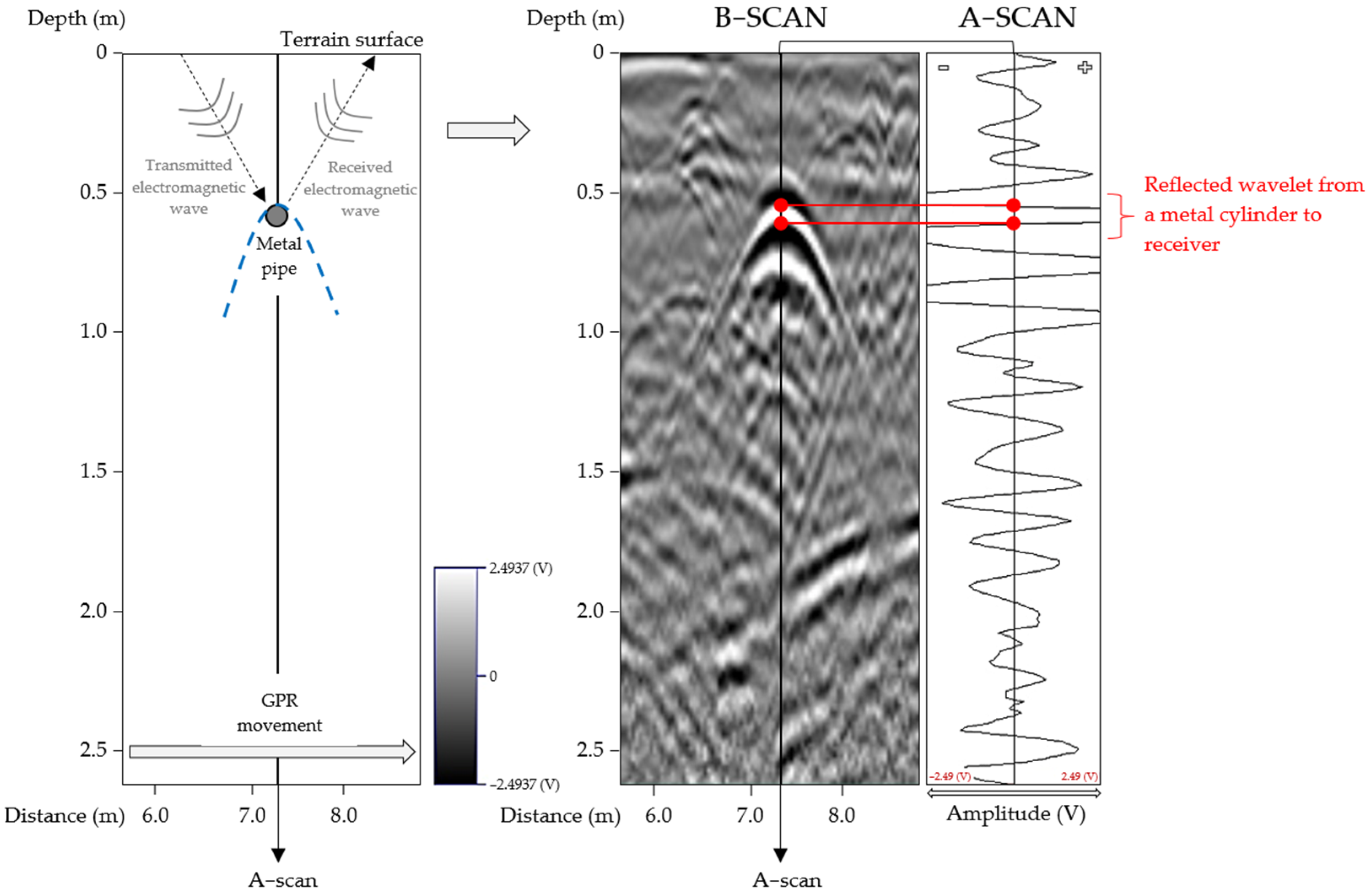
The location of the position of the buried object consists in determining the vertex of the hyperbola. Figure 1 shows the simplest case that presents the location of underground utility network. However, the interpreted fragments of radargrams do not always look like this. Sometimes, objects partly overlap, which makes it more difficult to conduct the process of automated segmentation and classification of objects in the image.
The original signal sent by the ground−penetrating radar forms the so-called A−scan matrix, which is presented in Figure 1. It is a set of reflected waves (recorded in the domain of time), captured along a vertical straight line crossing the ground at the given point. The B−scan images are sets of multiple A−scan images that represent the current information about underground objects. The process of their formation consists, among others, in mapping processed A−scan matrices to images in grayscale with 256 brightness levels.
2.3.2. Imagery Pre-Processing
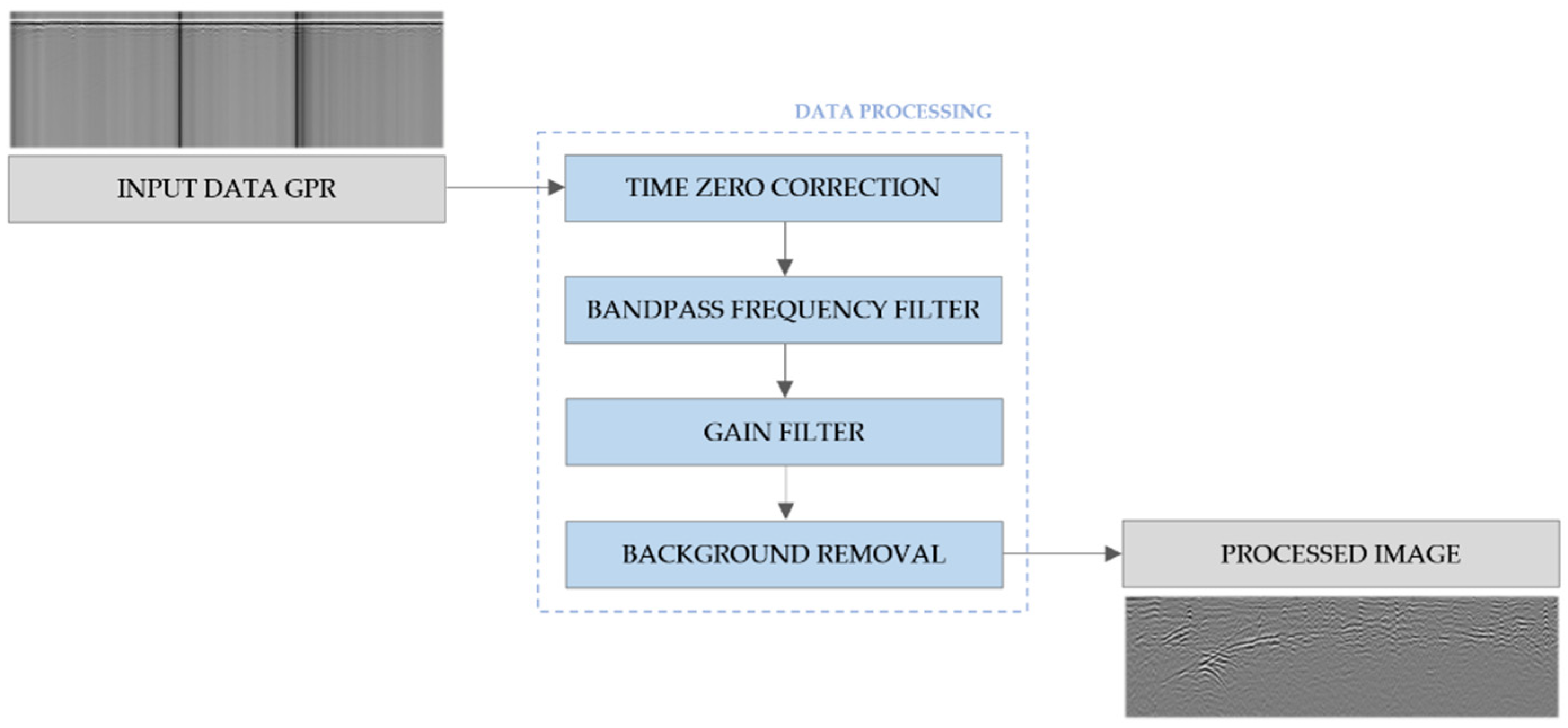
Radargrams obtained in the uNext software were pre-processed with the GRED HD software. This process consisted of the following stages: time zero correction, bandpass frequency filter, gain filter, and background removal. The range of the applied operations varied from 0 to 4.5 m. The results of every processing stage are presented in Figure 2. The aim of time zero correction is to adjust the zero time to the time on the surface of the Earth. The difference in time results from thermal drift, electronic instability, or variations in antenna airgap. In order to improve image quality and the signal to noise ratio, both time filters (i.e., simple mean, simple median, low pass, high pass, and band pass) and space filters (i.e., simple running average, average subtraction, and background removal) may be implemented [4]. One of the applied filtration processes consisted in conducting the Gain processing which refers to the enhancement of the amplitude and energy of electromagnetic waves, whose power diminishes after dispersion, diffraction, and absorption by the underground medium. If the signal of the return electromagnetic wave is weak, it may be enhanced with the function of exponential enhancement. At the next stage, background removal was conducted in order to eliminate random noise and to improve the signal to noise ratio. One of the final stages of processing of a radargram involves conducting migration and the correction of height and depth, whose value may be determined based on the velocity of propagation of the electromagnetic wave.
In the GRED HD software, the positioning and filtration systems are recognized automatically, and the filter parameters are selected individually for the dataset. Thus, standard processing of a radargram includes time-zero correction, removing the background, and frequency and gain filters. The software also enables individual selection of parameters, which was tested and confirmed in publications [34].
2.3.3. Candidate Objects
Candidate objects are a group of hyperbolas that were manually identified during the pre-processing of images and classified into three groups. According to Gauss normal distribution, we propose the following classification:
- G1—certain objects (the probability of representing the underground utility networks is on the level of ),
- G2—uncertain objects (the probability of representing the underground utility networks is on the level of ),
- G3—least certain objects (the probability of representing the underground utility networks is on the level of ).
For the purposes of classification and meeting the condition of probability, we analyzed that the following radiometric and geometric conditions should be taken into account:
- curvature of the object—CC,
- radiometry—CR,
- size of the object—CS,
- depth—CD, and
- length of the object’s arms—CL.
The probability of the existence of a buried object is related to the degree of fulfilment of the specified criteria 1–5. In group G1, properties 1–4 were important. Objects classified into group G2 were different from those from G1 because of the lower significance of properties 1 and 4. Group G3 is characterized by lower significance of properties 1–3 in comparison to groups G1 and G2. The differences between classes result from the information content in the images generated as a result of applying methods in figures, including the content of noise and basic information. These conditions (1–5) were defined based on the analyses of test images, and their results were verified based on reference data of underground utility networks obtained from the NGCR. Our analyses revealed that the condition CL did not influence the correctness of detection or classification of hyperbolas, so it would not be taken into account in further analyses. The radiometrics condition includes such properties as brightness and contrast in the image and, in further analyses, it is also involved in the wavelet and filtration functions. Thus, it will not be applied directly in the classification equations.
2.3.4. The Manual Method
The obtained radargrams were subjected to manual (visual) analysis, which is a reference (comparative) method for the automated methodology that is proposed in the further sections.
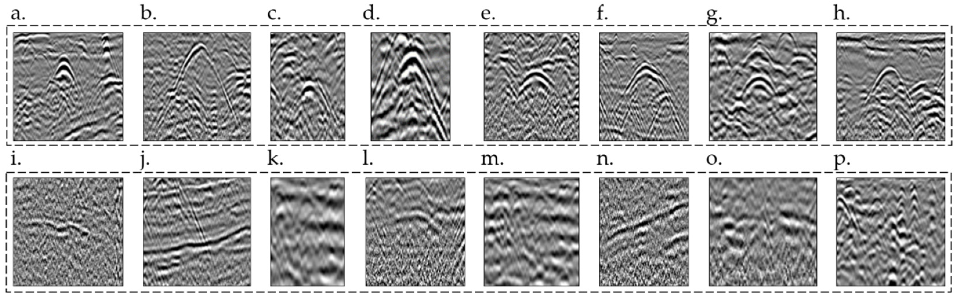
Figure 3 presents sample hyperbolas that were assigned to the group of candidate objects—true (Figure 3a–h) and false elements that were not taken into account in the conducted analyses (Figure 3i–p).
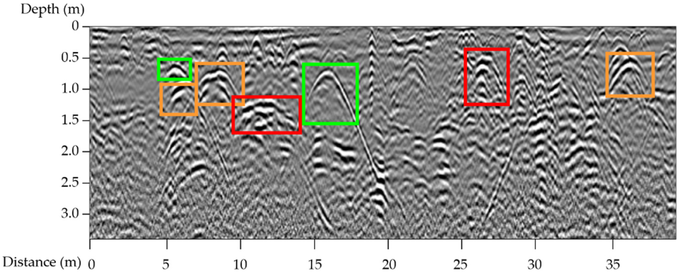
The hyperbolas selected manually in radargrams were then selected and assigned to one of three classification groups: G1–G3. Hyperbolas were marked in green (G1), orange (G2), and red (G3). Figure 4 presents an example of the selection of candidate objects on a fragment of the selected radargram obtained in the first measurement series.
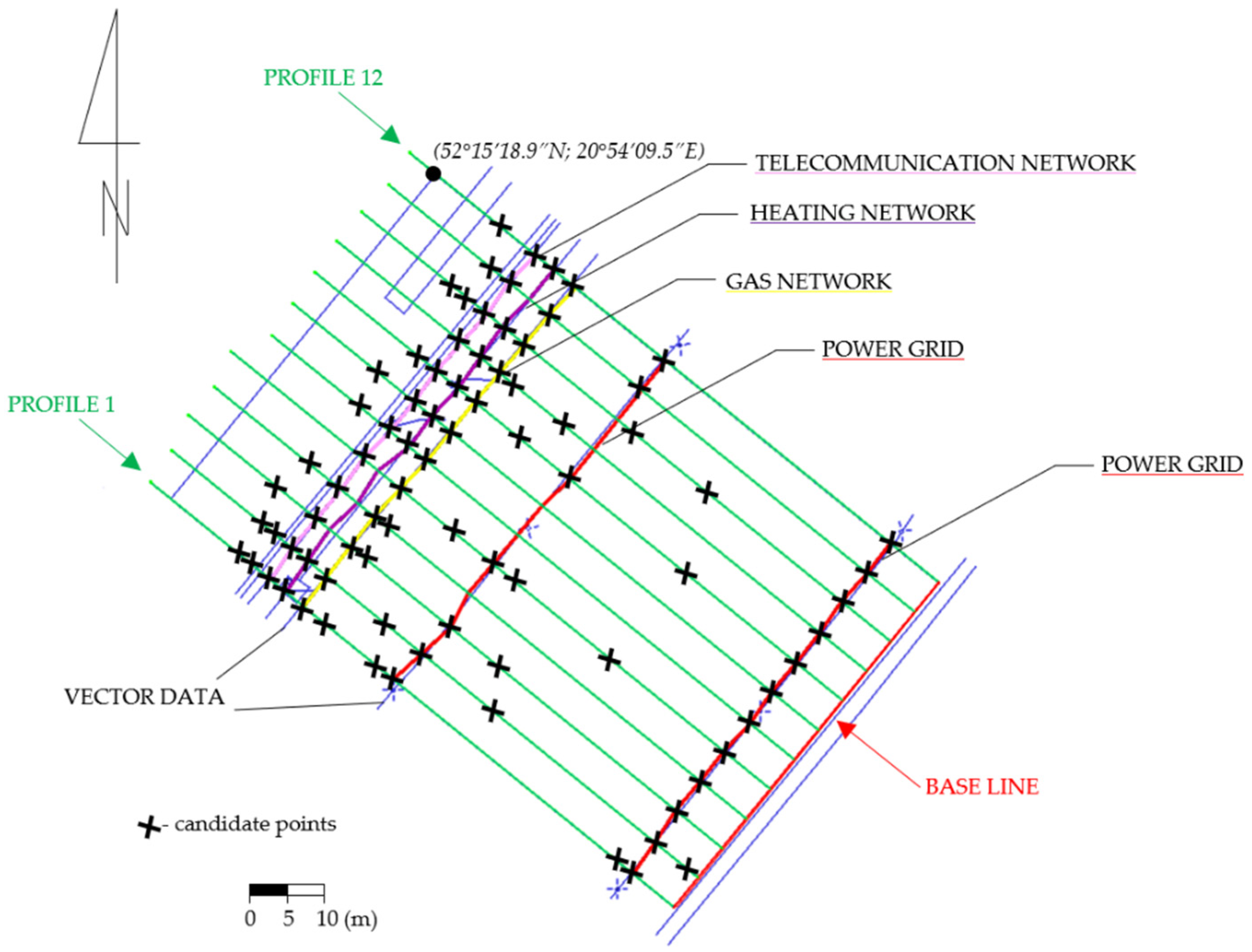
The reliability and correctness of the selection of candidate objects was confirmed by referring manual detection to reference data obtained from the NGCR. Figure 5 shows the analyzed area with the differences in the situational position of the underground utility networks between source data (from the NGCR) and manually selected points.
The difference between the coordinates of reference data obtained from the NGCR and the coordinates of candidate points does not exceed 0.22 m (for the power grid), 0.15 m (for the gas network), 0.35 m (for the heating network), and 0.11 m (for the telecommunications network). These difficulties are caused by, among other things, the accuracy of determining the georeference of data based on the GNSS receiver integrated with the ground-penetrating radar. The selected candidate points constitute reference data for the proposed methods in Figure 6 and Figure 7, whose results are presented in the Results section.
3. Proposed Methods
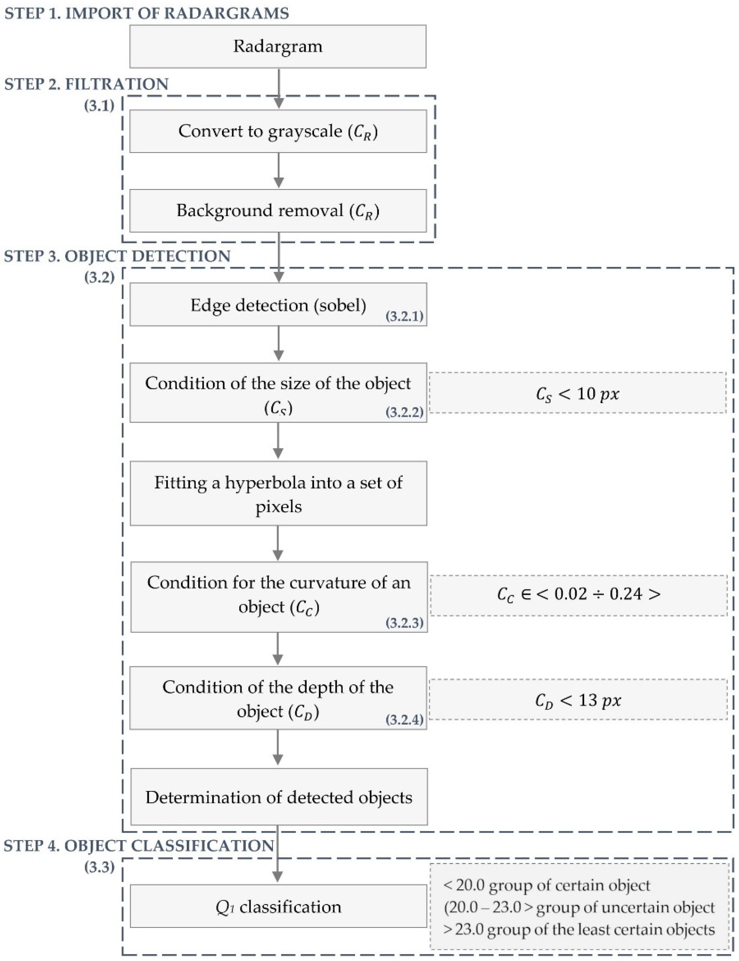
This section presents the methodology of the automation of the object classification process, i.e., an improvement of the process of selecting the true hyperbolas in the radargram. We have proposed two methods that consist of the image filtration stage and the stage of object detection and classification. Method 1 (Figure 6) is based on converting the RGB image to grayscale, background removal, edge detection, fitting the object into the set of detected pixels, and selecting only those hyperbolas that meet the predefined conditions:
- size of the object— (Section 3.2.2),
- curvature of the object— (Section 3.2.3),
- depth of the object—(Section 3.2.4).
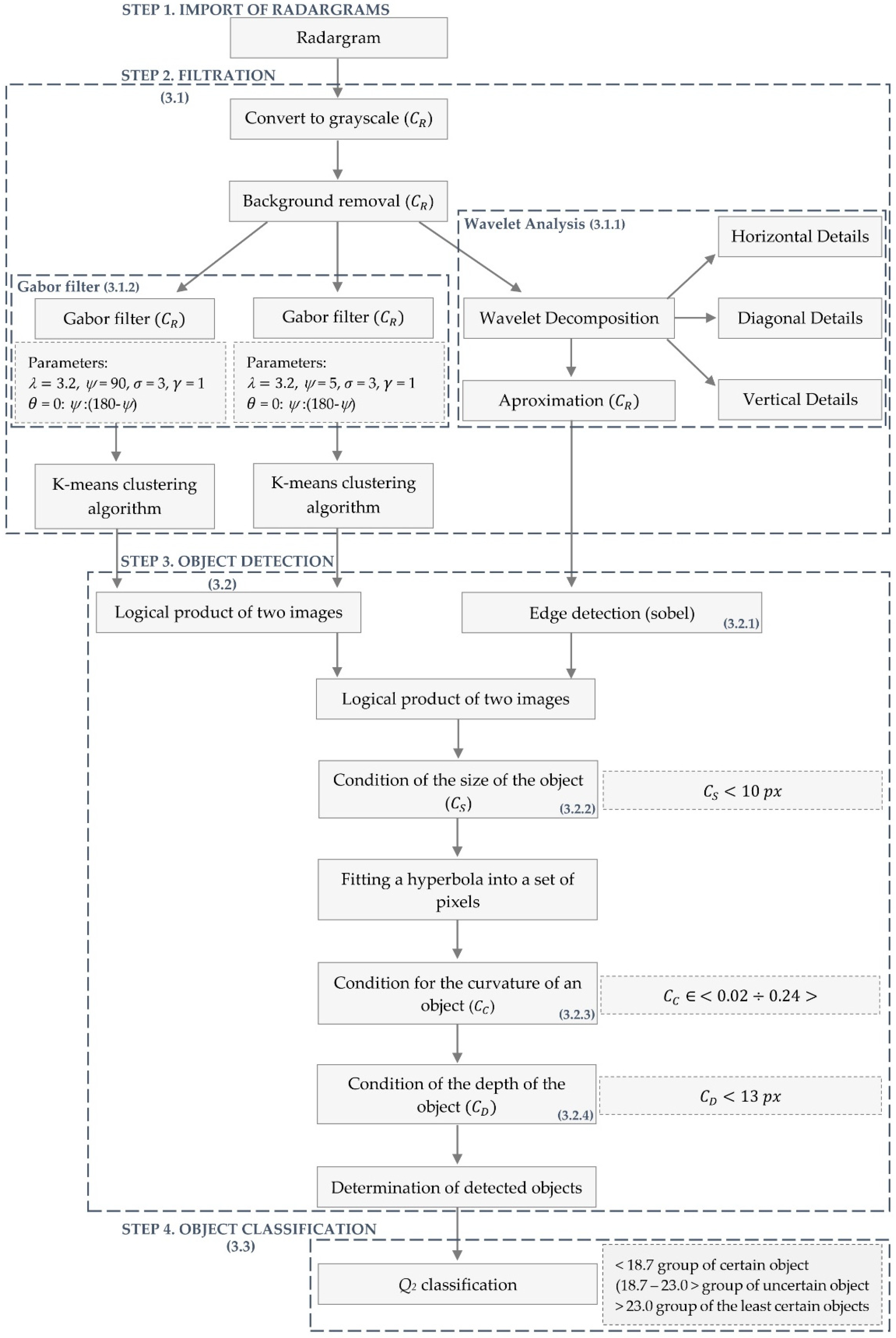
Method 2 (Figure 7) is based on image filtration (after pre-processing) with use of wavelet analysis, and, more precisely, image approximation at the set level of wavelet decomposition (level 1) and Gabor filtration with use of the parameters described in Section 3.1.2.
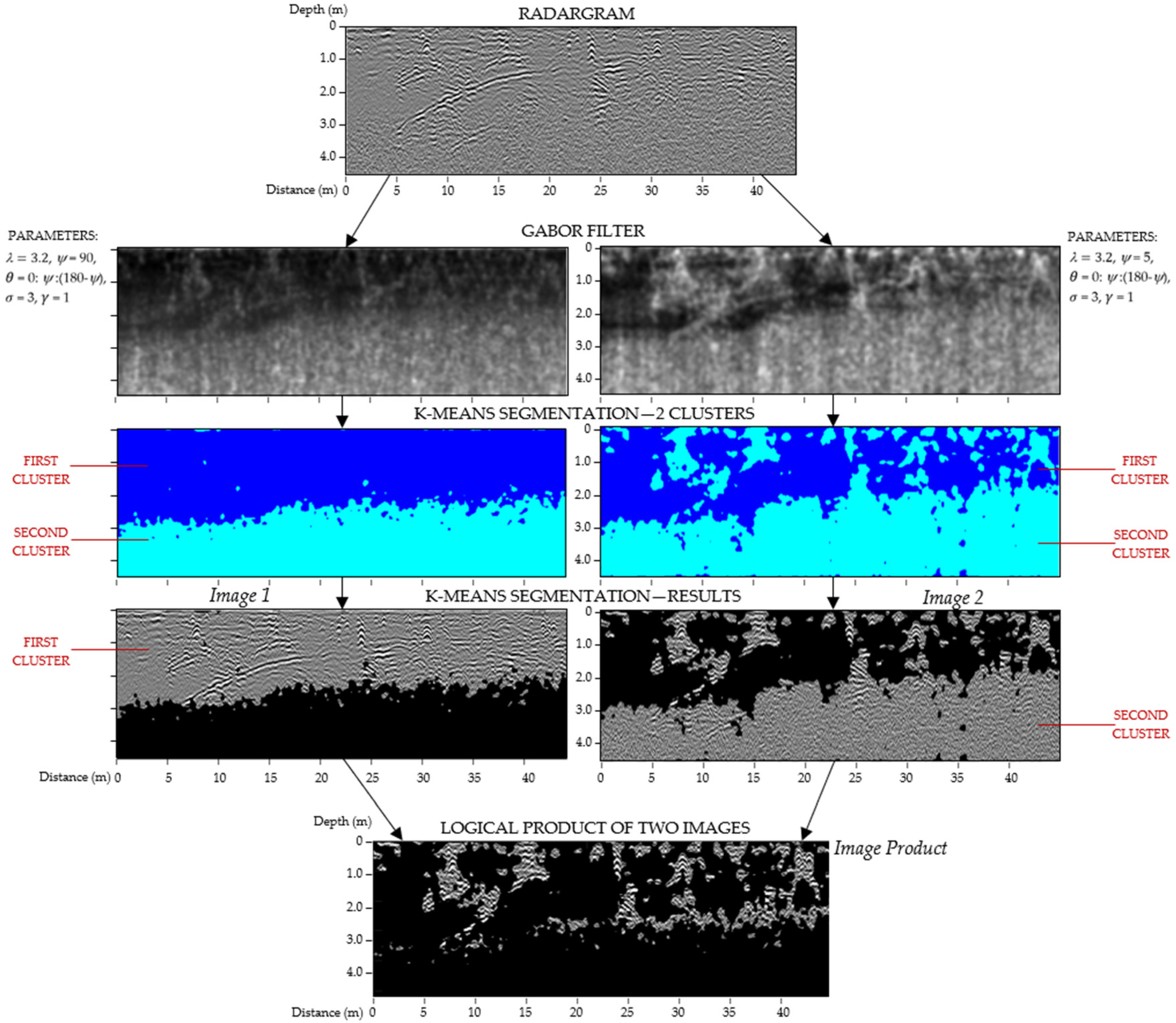
As a result of Gabor filtration of the given radargram, two different images were obtained, which were subjected to K-means clustering. As a result, fragments of two radargrams were selected that represented objects of the highest value of pixel brightness Digital Number. The target image was based on the logical product of these two radargrams. At the same time, the radargram (after pre-processing) was subjected to wavelet analysis, which is discussed in detail in Section 3.1.1 (stage 2). The method uses only the approximation of the image based on the Symlet5 wavelet from the image decomposition process. Edges were detected in the filtered image with use of Sobel operator (Section 3.1.1). After introducing the condition of object size, a logical product of two images obtained in the first and second stage was conducted. At the subsequent stages, the hyperbola was fitted into the set of pixels and the conditions of object size, curvature, and depth were introduced, which resulted in determining the potential target objects.
3.1. STEP 2—Filtration (Method 2)
3.1.1. Wavelet Analysis
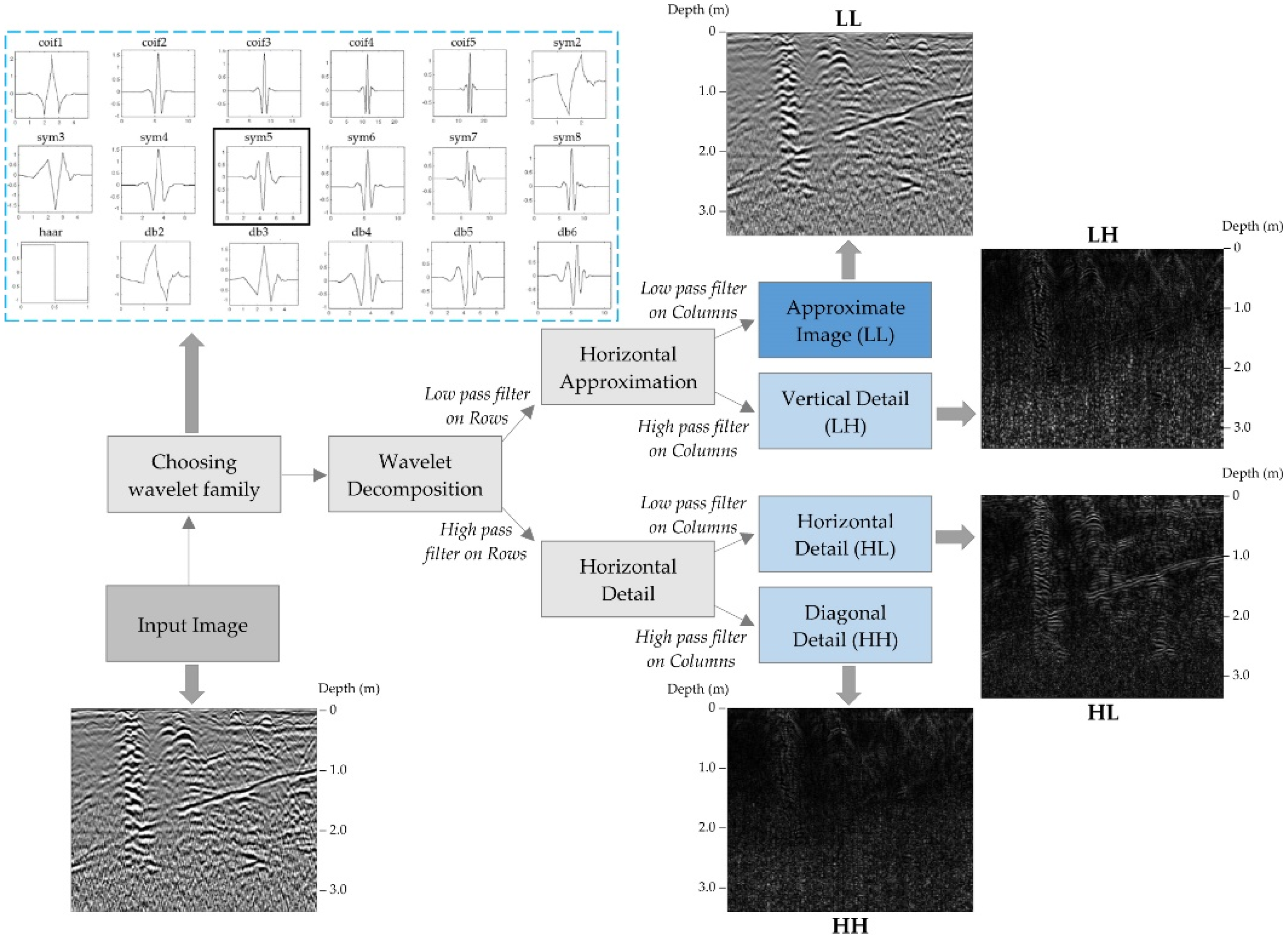
Wavelet analysis is based on the decomposition of the image (or wavelet development of the image). As a result, four components are obtained: approximate image and details (vertical, horizontal, and diagonal detail). Image decomposition consists in high- and low-pass filtration, which is a multi-level iterative process, in which each approximate image may be subjected to further decomposition. The detail components obtained as a result of wavelet decomposition represent high-frequency components, which highlight the horizontal, vertical, and diagonal edges. The approximation of the analyzed image represents the low-frequency component obtained after the removal of details [35]. The diagram of image decomposition is presented in Figure 8.
Based on the above illustration, one may notice that the image approximation was obtained by means of applying low-pass filters on rows and columns. Vertical details were distinguished as a result of applying low-pass filtration on rows and high-pass filters on columns. The reverse combination of filters resulted in the horizontal details, while diagonal details were obtained after applying high-pass filters on rows and columns [36].
The initial stage that commences the wavelet analysis of the obtained data is the selection of the decomposing mother wavelet and the decomposition level that depends on the length (N) of the given series (signal) [37].
Subject literature provides several methods that allow to determine the maximum decomposition level () of a one- or two-dimensional signal (image) based on empirical tests or theoretical knowledge, i.e., among others based on entropy or from the equation [36].
Another important aspect is the selection of the mother wavelet that depends on the shape and properties of the signal. Usually, the appropriate wavelet is selected in an empirical process. In the present study, after testing Haar, Daubechies, Symlet, and Coiflet wavelets on radargrams, Symlets wavelets were selected as those best fitting into searched objects (hyperbolas) and the first level of decomposition.
3.1.2. Gabor Filter
The analysis of textures in images often employs the linear Gabor filter, which analyzes the content of the frequency predefined by user at the set directions (oriented filtration) in the analyzed area [27]. The Gabor filter is defined by Equation ((5)–(7)) in the general form:
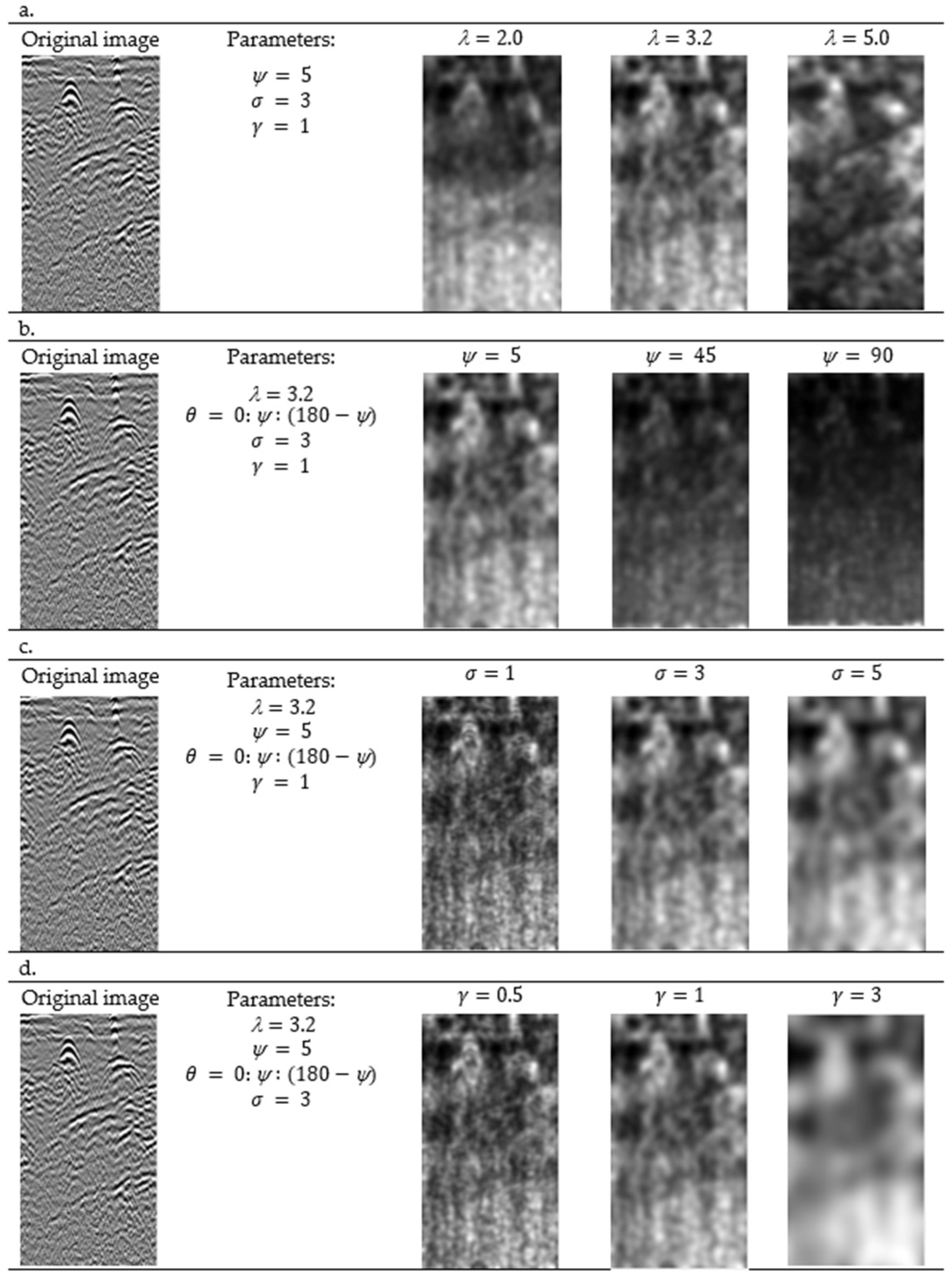
The parameters used in Equation (5) denote the wavelength of the complex sinusoid (), the orientation with respect to the normal (), the phase offset (), the variance of the Gaussian envelope (), and the aspect ratio (). In the representation of the function, light pixels represent the positive values and dark pixels the negative values of the function. Dark areas represent frequencies with a small or zero power spectrum, while areas with light pixels represent frequencies with a significant power spectrum.
The wavelength is denoted in pixels and it should take values exceeding 2. Along with the increase in , the area of pixels that correspond to positive values of the function increases. The parameter is the orientation of the normal line with respect to the parallel stripes of the Gabor function. Its value is usually presented as 0°, 45°, 90°, and 135° [38]. The parameter is the phase offset of the cosine of the function and it takes values in the range from −180 to 180 degrees. The variance of the Gaussian envelope () defines the linear dimension of the receptive field in the image and the eccentricity of this area is defined by the aspect ratio (). A selective modification of the parameters of the Gabor function allows adjusting the filter to specific patterns of objects represented in the image. Figure 9a–d present the target images subjected to Gabor filtration with different parameters at varying parameter values: (Figure 9a), (Figure 9b), (Figure 9c), and (Figure 9d).
The obtained test images were subjected to Gabor filtration twice. First of all, fragments of radargram with the highest differences in pixel brightness were selected based on the values of the parameter —Equation (8).
Then, areas were selected for which data had not been obtained due to the dielectric properties of the media and significant depth of detection. The parameters were used—Equation (9).
Filtration parameters were selected in a way that would ensure the highest degree of detection of true objects while, at the same time, minimizing the detection of false objects (Figure 9). The aim of applying the appropriate values of Gabor filtration parameters is to distinguish the hyperbolas that constitute the location of potential underground utility networks.
3.1.3. K-Means Clustering
The segmentation of the filtered image is applied in order to distinguish objects of selected properties [39]. This process may be performed with use of supervised classification or unsupervised classification. One of the most popular methods of separating clusters is the k-means clustering method that was applied in this study. The selected type of segmentation process automatically groups the pixels in the property space. The k-means clustering method is based on iterative separation of selected pixels whose initial mean vector is assigned freely for each of the two clusters. At the subsequent stage, each pixel of the image is assigned to a group where the mean vector is the closest to the pixel vector. This process is then repeated until the differences in pixel classification between iterations become slight (10) [40,41].
where:
—object class,
—iteration number.
Figure 10 presents a sample image subjected to Gabor filtration twice (with the parameters discussed in Section 3.1.2) and segmentation of elements of the defined textures. As a result of filtration and segmentation, the operator obtains two images: (from filtration with parameter ) and (from filtration with parameters ).
The segmentation of an image that was previously subjected to Gabor filtration divides it into N clusters selected by the operator. We divided it into two parts. A logical product of the images obtained as a result of double segmentation was calculated (Equation (11)) to distinguish the intersection of both images and (Figure 10).
This stage enabled us to distinguish the objects of defined textures (the true hyperbolas) in form of radargram fragments, which were then subjected to further analyses.
3.2. STEP III—Object Detection
The detection of hyperbolas in radargrams consists of several stages, i.e., edge detection (Section 3.2.1), fitting the hyperbola into the set of pixels, and partial removal of objects by 3 introduced conditions: (Section 3.2.2), (Section 3.2.3), and (Section 3.2.4).
3.2.1. Edge Detection
From all the existing methods of image segmentation, the edge detection methods have been applied. This choice was dictated by the ultimate detection of edges of the true hyperbola that constitutes the potential location of an underground object. The application of Sobel edge detector that was used in all methods enables to generate gradient images. The detector employed by the method allows the estimation of image noise based on the value of square mean. The Sobel operator determines the horizontal and vertical gradients based on finite differences. It is based on averaged discrete derivative, where the weight of the derivative value (which is calculated through the mean) is twice as large as the derivative calculated from neighboring elements [42]. After the edge detection process, the user receives a binary image, i.e., an image that contains only pixels of the values of 0 and 1.
3.2.2. The Condition of the Size of the Object (
The condition of the size of the objects represented in the image was introduced in order to remove single pixels and small elements that are insignificant in the process of detecting underground utility networks. Based on the analysis of radargrams, it was found that the significant size of true objects is 10 px, which corresponds to the multiplication by 1.5–2.5 (depending on the type of underground network). The size threshold () of objects was defined based on empirical studies on 10 test images introducing condition (Equation (12)).
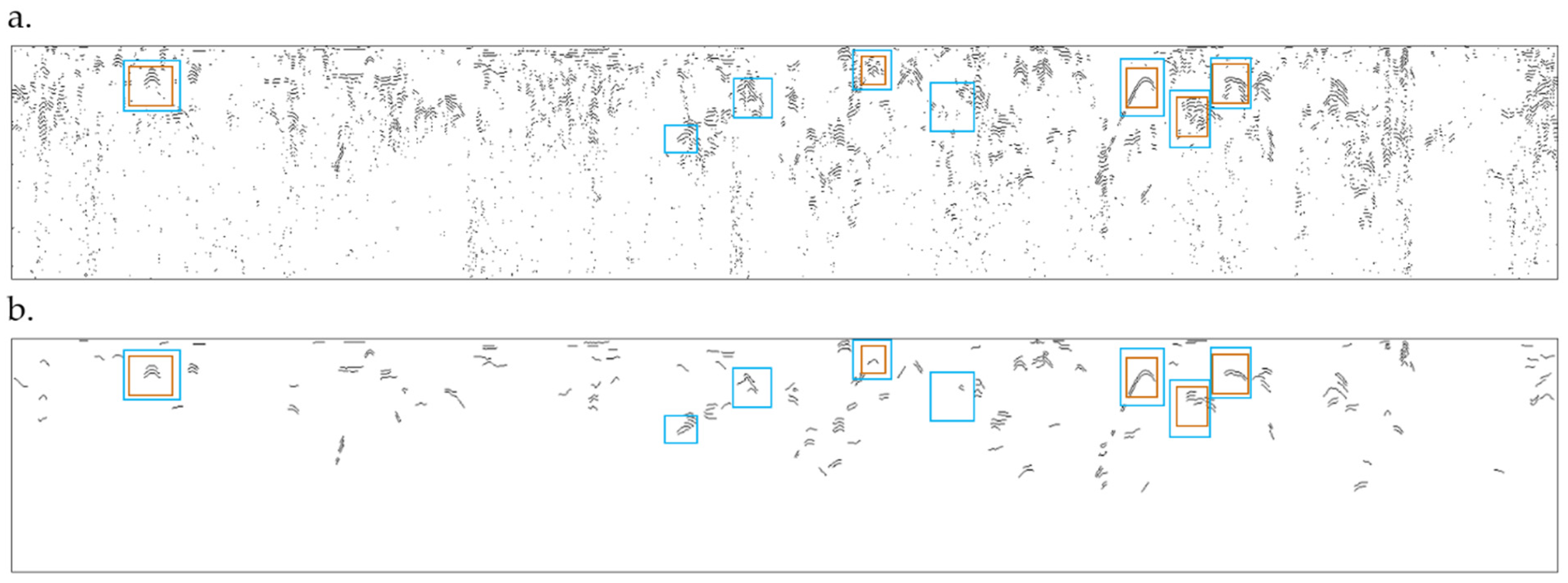
Figure 11a,b present the image before (Figure 11a) and after (Figure 11b) the introduction of the object size condition, with candidate objects marked in blue and the existing underground utility networks according to source materials from the NGCR marked in brown. The results of the introduced condition of the size of the buried object are presented on a sample image (obtained on measurement route 11, in the 4th measurement series).
The elimination of small elements allowed us to distinguish only those objects that are significant for further analyses taking into account the curvature of the object or the depth of its location.
3.2.3. The Condition for the Curvature of an Object (
In order to introduce the condition for the curvature of the object to the method, first of all the values of the a, b, and c coefficients had to be determined for each parabola in the image, and then it had to be fitted into the set of pixels corresponding to each detected object.
The direction coefficient a, in the form of a general square function, defines the direction in which the arms of the parabola are pointing. The coefficients a, b, and c of the equation (Equations (17)–(19)) may be determined based on the coordinates x, y of at least three specific points of the given object and matrix determinants (Equations (13)–(16)).
The determination of the a, b, and c coefficients of the parabola equation and the process of fitting it into the set of obtained pixels with use of the non-linear least squares method was conducted in the Matlab software. The search for the optimum points starts with the initial approximation, through subsequent iterations of obtained approximations that are close to the optimum estimate according to the least squares method. Based on the defined parameters of the independent variable x, the method determines a set of a, b, and c coefficients for each object detected in the image (Equations (17)–(19)).
The range of values of the direction coefficient a was calculated based on multiple determinations of its value in test images and the available materials and information obtained from the NGCR. This allowed for a reliable determination of the range of curvature of true objects. Iteration tests resulted in the determination of the value of the direction coefficient a (Equation (20)) for all 60 images. Regardless of the radiometric span of the image, the range is constant and correct for all radargrams.
The detected objects whose curvature lies beyond this range will be eliminated at the stage of introducing this condition to the given method. The table below presents direction coefficients for both true and false underground objects (tested on 10 images).
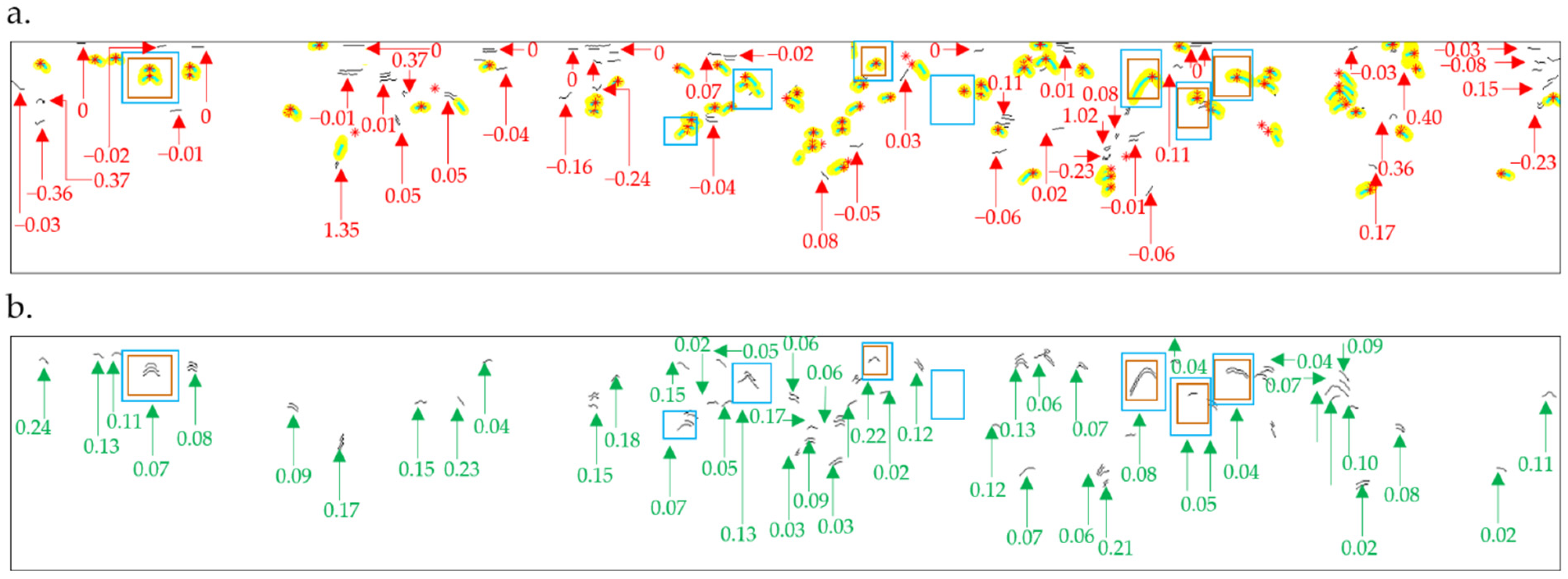
The results of the introduced condition for the curvature of the buried object are presented on a sample image obtained on measurement route 11, in the 4th measurement series (Figure 12a,b). Objects whose curvature falls in the range determined above are marked in green and yellow. The values of the a coefficient for candidate objects, including the existing underground utility networks, are marked in green. Black color (in Figure 12a) marks the objects whose curvature does not fall into this range. The values of the coefficient for the eliminated objects are marked in red.
The effectiveness of the removal of false objects after introducing the condition for curvature for the sample image (radargram 11, measurement series 4) tested with Method 1 was 48%. The method initially detected 189 elements, 91 of which were eliminated by the condition for curvature. The results of the effectiveness of elimination of false objects were analyzed for 10 radargrams obtained in the 4th measurement series and presented in the Results section.
3.2.4. The Condition of the Depth of the Object (
The legal basis for the determination of the criterion of the depth of the location of an underground object is technical guidelines. They contain the minimum values of cover thickness for underground network installations according to their type (Table 2).
Assuming that the underground utility network is detected in an area where the operator does not know the position of the given objects, the minimum depth (common for all types of networks) is 0.5 m. The underground utility networks in the analyzed area are located at the depths ranging from 0.65 m to 1.21 m. The aim of the introduction of the condition of the depth of the object is to partly eliminate false objects located at small depths and the noises in these areas. In order to determine the minimum depth of the location of the object, a small margin of error should be introduced, of the value of approximately 15 cm.
The proposed method eliminates hyperbolas whose vertex depth is smaller than 13 px (it is the equivalent of the Y ordinate, the depth of the location of the object), which corresponds to roughly 35 cm. The value of the introduced criterion (in pixels) was calculated based on a specific vertical resolution, which was determined based on antenna frequency, the rate of propagation of electromagnetic waves, and relative dielectric permittivity (Equations (21) and (22)).
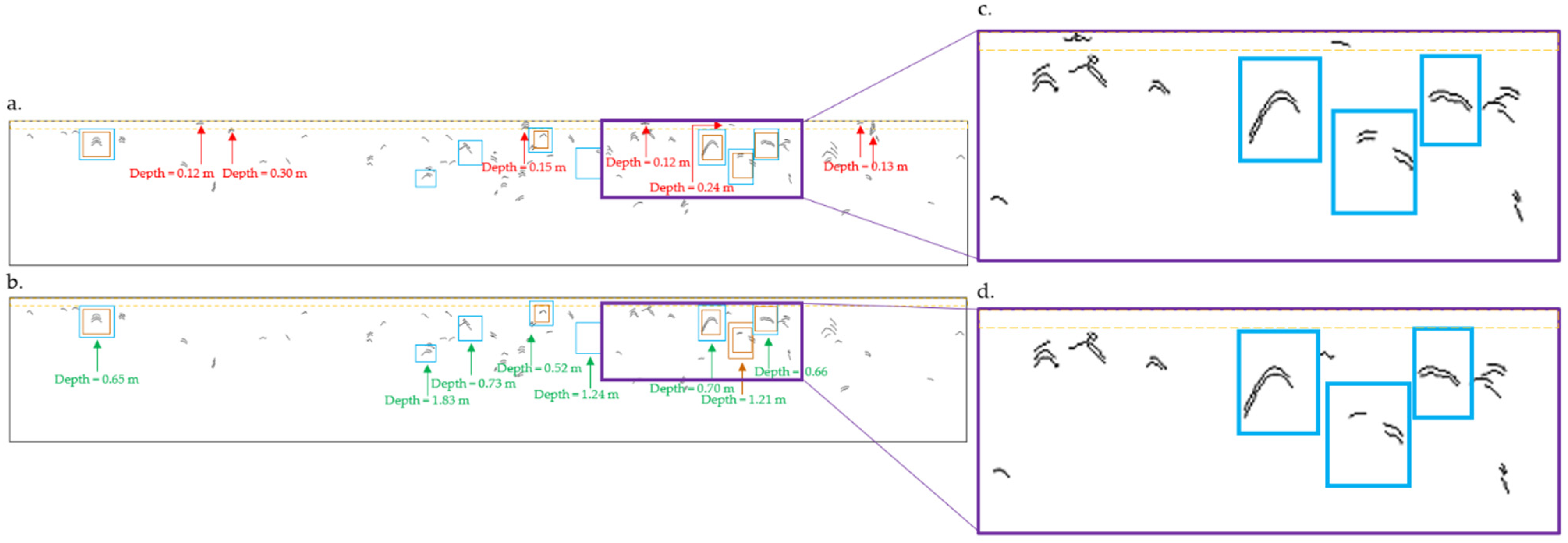
Figure 13a,b present the result of the application of Method 1 after introducing the condition of the depth of the underground object, which eliminated objects located at a depth lower than 13 pixels, based on the example of measurement route 11 obtained in the 4th measurement series. The area marked with the dotted line in Figure 13a,b is the range of the occurrence of condition in the image. Objects situated in this area are eliminated after the introduction of condition . Figure 13c,d are magnified fragments of Figure 13a,b.
Figure 13a shows the detection result before introducing this criterion, and Figure 13b after taking it into account. Objects that are eliminated after introducing the condition of the depth of the object are marked in red, while the depths of manually selected buried objects (candidate objects) are marked in green.
3.3. STEP IV—Proposed Method of Automated Classification of Objects in the Image
The developed method of the classification of objects in images takes into account the values of the three conditions introduced to the method: the conditions for the curvature, depth, and size of the object (Equation (23)). The result of the Q classification criterion for the given element constitutes the basis for the determination of the degree of significance of the object in the classification process. The weights presented in Equation (23) were introduced based on the analysis of 10 test images. The Q classification criterion automates the classification process by making the selection more effective by increasing the certainty of its occurrence.
where:
—condition for the size of the object,
—condition for the curvature of the object,
—condition for the depth of the object,
—weight coefficients.
The values of variable weight coefficients () may be determined with the use of statistical methods or substantive analyses. Calculating their values is important for the final evaluation of the object. Substantive methods are based on the perception of the operator, who assigns weights of a total of 1 or 100 to the collected variables. The problem of the perception capacity of the analyst may be solved by determining the weights of attributes with use of the analytic hierarchy process (AHP) [43,44,45].
The AHP method is based on the determination of a weight multiplier that corresponds to the characteristics of the given element. The aim of the multiplier is to put the properties of the objects in order. The attributes analyzed in the study are the curvature, size, and depth of location of the buried object. The weights of attributes are recorded in form of a matrix of comparisons (Table 3). The diagonal of the matrix contains the number 1 as the attributes are evaluated in comparison to themselves. Higher values of the weight multiplier will be assigned to attributes of higher significance in comparison to other properties of the object [46].
The measures of significance in the matrix of comparisons were determined according to other studies [45] based on [47,48]. Article [45] contains the degree of significance of the given factors and their explanations (Table 4).
The AHP method is an approach based on criteria hierarchization, which is one of the branches of multi-criteria optimization. The method, developed by Thomas Saaty in 1980, consists in weighting elements on each level, which leads to approximation (Equation (24)) [48,49]. Its results are presented in Table 9.
where:
—value of the weight of element i,
—value of the weight of element j.
The estimated weight vector is determined by solving the following eigenvector problem based on Equation (25) [46].
where:
—matrix containing the values ,
—main eigenvalue of matrix A.
For the purposes of the classification of objects detected in the image, the simplified AHP method was used. One of its stages, following the development of the matrix of priorities, is the normalization of the obtained results in specific columns . This step involves dividing each of the elements in the table by the sum of values of the elements contained in the specific column (Equation (26)). The calculated values of the normalized matrix are presented in Table 9 (Section 4).
where:
—number of elements in the given row.
The values of the weight coefficient are calculated by adding the given elements in rows and calculating the mean (Equation (27)) [48].
4. Results
This section presents the results of the application of the proposed methods for test images. Section 4.1 contains the results of the effectiveness of detecting candidate points after the elimination of objects by the introduced conditions (, ). It is important to maximize the removal of false objects, while, at the same time, maximizing the degree of detection of all significant objects. Section 4.2 provides an assessment of the effectiveness (Section 4.2.1) and quality (Section 4.2.2) of the detection of hyperbolas being underground utility networks. Further on, Section 4.3 contains a presentation of the results of the obtained values of weight coefficients of attributes and an assessment of the compliance of the classification of underground objects in the image with the reference data of the detection of hyperbolas being underground utility networks. Further on, Section 4.3 contains a presentation of the results of the obtained values of weight coefficients of attributes and an assessment of the compliance of the classification of underground objects in the image with the reference data.
4.1. Results of the Detection of Candidate Objects after the Introduction of Conditions
The introduced conditions (, ) in correctly defined ranges remove part of the objects that were initially detected. At this stage, it is important that the manually determined candidate points should not be eliminated after the introduction of specific conditions. Figure 14 shows the final hyperbola detection result on the GPR images for Method 1 in Figure 14a and Method 2 in Figure 14b.
Table 5 contains the results of the effectiveness of detection of candidate objects in target images after the implementation of the criteria. The results refer to the application of methods in Methods 1 and 2 and to images obtained in various measurement series at different times of day and on different measurement routes.
The aim of the proposed methods is to detect the highest possible number of true objects and at the same time to eliminate falsely detected elements. In order to compare the proposed methods for test images (Table 5), the SNR (signal to noise ratio) was calculated (Equation (28)). The higher the value of this coefficient, the better the results obtained with the given method.
where:
—number of detected candidate objects,
—number of detected false objects.
Table 5 demonstrates that the average effectiveness of detection of candidate objects (after the introduction of the three conditions described above) fell into the range of 89–100% for Method 1 and 80–100% for Method 2. Higher effectiveness of detection may be obtained with use of Method 1. However, it contains a larger number of objects, which introduce noise and interfere with the correct selection of target objects. The average effectiveness of detection for 10 analyzed images was 99% for Method 1 and 89% for Method 2.
The above results demonstrate the repeatability of detection in different series in the corresponding measurement routes 80–87% (route 3), 83–100% (route 6), and 83–100% (route 11). The average effectiveness of detection of candidate objects for Method 1 was 96% (for series 1), 100% (for series 2), 100% (for series 3), and 100% (for series 4), and for Method 2 82% (for series 1), 91% (for series 2), 80% (for series 3), and 96% (for series 4). The presented results allow us to draw the conclusion that Method 1 offers higher effectiveness of the detection of underground utility networks. On the other hand, Method 2 is characterized by a higher effectiveness of the elimination of false objects than Method 1, which was confirmed by the values of the SNR coefficient presented in Table 5. The values of the SNR coefficient for Method 2 are twice as high as for Method 1.
4.2. Evaluation of the Effectiveness and Quality of the Detection of Hyperbolas
4.2.1. Evaluation of the Effectiveness of the Detection of Hyperbolas
The effectiveness of the detection of hyperbolas in GPR images (coefficient M in Equation (29)) was evaluated by comparing —the number of objects detected in the target image (i.e., after the -processing stage, filtration, and the application of conditions , ) and —the number of objects detected in the output image (i.e., after pre-processing).
The values of M (Equation (29)) were calculated for the results obtained from 10 radargrams, and the obtained average values are presented in Table 6.
The obtained values of M show the percentage growth of detection effectiveness caused by partial elimination of false objects. The obtained M values for Methods 1 and 2 confirm the previously calculated SNR value, which demonstrated that images obtained with Method 1 contain more noise than those from Method 2. Detailed results are provided in Appendix A.1 to the publication.
Moreover, Equation (30) was used to calculate the percentage of true objects in all objects detected in the target image (based on reference data). This value (L) was calculated for 10 target images obtained from Methods 1 and 2, and the obtained average values are presented in Table 7. Detailed results are provided in Appendix A.2 to the publication.
where:
—number of all detected objects in the target image,
—number of detected hyperbolas not being underground utility networks,
—number of not detected hyperbolas being underground utility networks.
The obtained results presented in Table 7 demonstrate that the target images obtained with use of Method 1 contain a higher number of false objects. The number of true objects obtained as a result of the application of Method 2 is twice as high.
The average effectiveness of detection of true hyperbolas, not considering , objects was 99% (Method 1), 97% (Method 2), and 92% (manual detection).
4.2.2. Evaluation of Quality of the Detection of Hyperbolas
The compliance of the detection of hyperbolas obtained as a result of the application of the proposed methods was evaluated based on the juxtaposition of parameters Precision (P), Recall (R), and determined for specific methods (Equations (31)–(33)).
where:
TP—true hyperbolas,
FP—false hyperbolas erroneously detected as true ones,
FN—true hyperbolas erroneously detected as false ones.
The results of Method 1 and 2 and of manual detection were referred to the reference data obtained from the NGCR. The values of parameters were calculated for the results obtained from 10 radargrams and the obtained average values are presented in Table 8. Detailed results are provided in Appendix A.3 to the publication.
The values of the P and R coefficients fall into the range . The higher the value of , , and , the higher the precision and recall of the proposed methods. Results provided in Table 8 demonstrate that the precision of Method 2 was twice as high as that of Method 1 and 4.5 times lower than that of manual detection. The highest value of the coefficient was obtained for Method 1, and the lowest for Method 2. The parameter provides an overall evaluation of the quality of the detection of hyperbolas in the image, taking into account the and coefficients. The quality of detection obtained in Method 2 was twice as high as for Method 1 and 3 times lower than in manual detection.
4.3. Results of Object Classification According to the Q Optimization Criterion
The obtained values of weight coefficients are presented in Table 9. The normalized values from the table were added to obtain the following average values: 0.52, 0.24, and 0.24.
These averages are the weights of the given criterion (Equation (34)).
For the results obtained with Method 1, the following ranges ( are proposed for the classification of objects detected in the radargram:
- For certain point (G1′),
- For uncertain point (G2′),
- For least certain point (G3′).
For the results obtained with Method 2, the following ranges () are proposed for the classification of objects detected in the radargram:
- For certain point (G1″),
- For uncertain point (G2″),
- For least certain point (G3″).
The resulting new values of the ranges were verified based on the determination of the degree of compliance of classes (G1′, G2′, G3′, G1″, G2″, G3″) determined by coefficients and in comparison to visually (manually) determined ranges and candidate points.
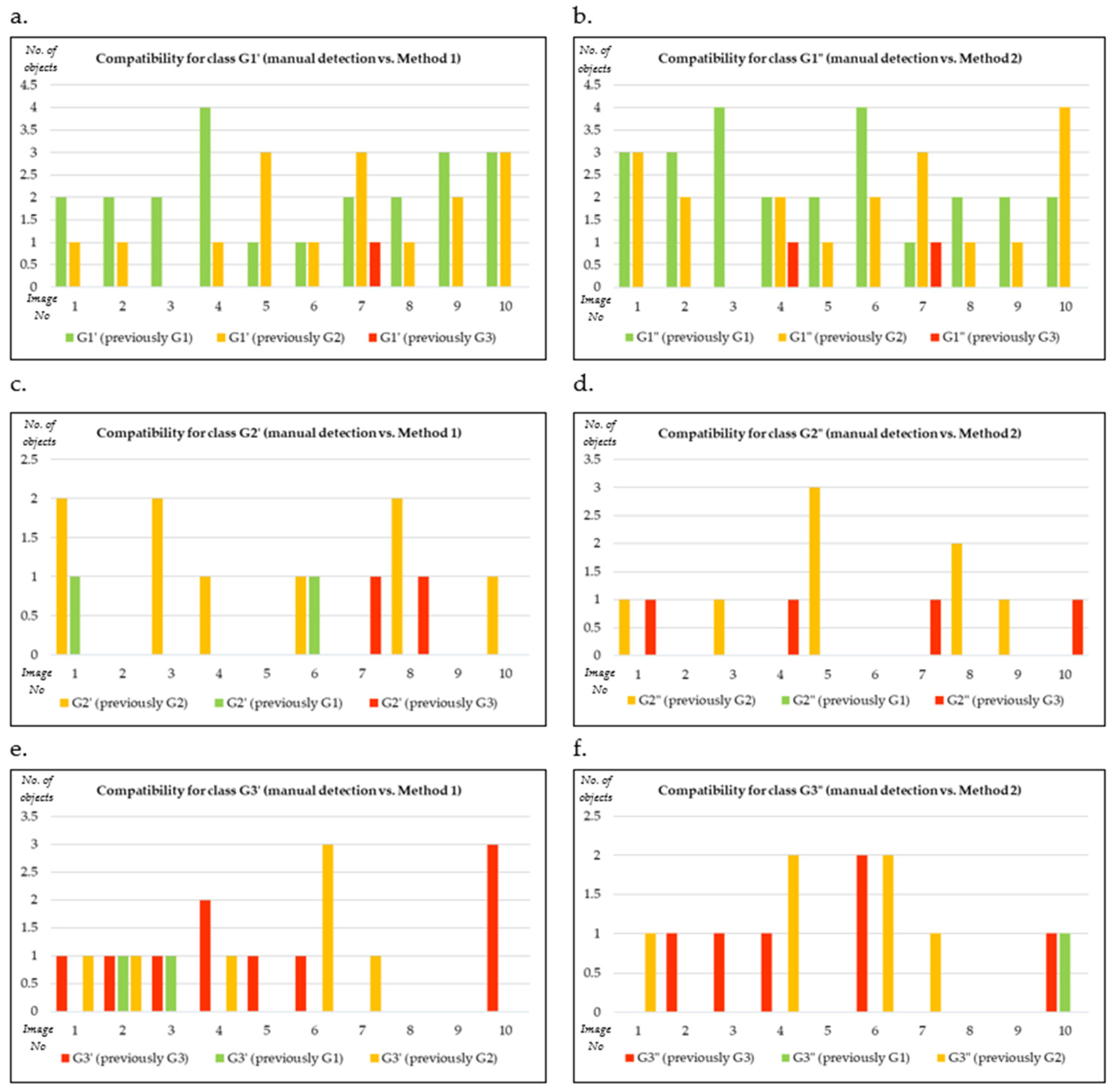
The diagrams below show the results of the compliance of classification of the detected hyperbolas (obtained with use of Method 1) with groups of certain objects (Figure 15a), uncertain objects (Figure 15c), and least certain objects (Figure 15e). The diagrams also show objects that were classified falsely with respect to reference data. Similarly, points b, d, and f (Figure 15) present the results of the compliance of classification of the elements detected in images obtained as a result of the processing with use of Method 2.
We propose to calculate the effectiveness of the classification of hyperbolas () with use of the and coefficients, based on Equations (35) and (36). It is assumed that if one of the factors (G or G′ or G″) equals 0, then the effectiveness of classification is also zero. The average values of the effectiveness of classification of hyperbolas and obtained for 10 images are presented in Table 10. Detailed results are provided in Appendices to the publication.
Assuming that: , ,
For , , :
where:
—classification groups: G1, G2, G3 (manual method) for i = 1, 2, 3,
—classification groups: G1′, G2′, G3′ (Method 1) for i = 1, 2, 3,
—classification groups: G1″, G2″, G3″ (Method 2) for i = 1, 2, 3,
—effectiveness of the classification of hyperbolas obtained from compared to manual classification,
—effectiveness of the classification of hyperbolas obtained from compared to manual classification.
The analysis of the results presented in Table 10 reveals that certain objects were classified (in comparison to manual detection) on the level of 58–60%. The lowest effectiveness of classification was noted for uncertain objects, whose parameters are on the boundary between classes both in the visual perception in the manual method and in the proposed automated methods. This results from the fact that a vast majority of objects in this class have a radiometric and geometric structure that is difficult to determine.
5. Discussion
The conducted research enables the automation of the process of detection and classification of underground objects in radargrams. As far as the practical application of the proposed methods is concerned, the operator may, on the one hand, obtain the final results in form of the coordinates of the vertexes of the detected hyperbolas, and on the other hand, they have the possibility to display all the sub-stages of filtration, detection, or classification of objects and perform manual selection. It is also possible to choose the method that will be used. Each of the proposed methods has several advantages, but also disadvantages.
One of the main advantages of the presented methods is the shortening of the GPR data processing time and of the interpretation of radargrams. The automated methods for the detection and classification of hyperbolas in GPR images made it possible to shorten the image pre-processing time by approximately 60%, the time of detection of hyperbolas by approximately 50%, and the time of classification by approximately 30%. Considering all three stages, one may notice that the application of methods allows shortening the total duration of work by approximately 45%. Apart from that, the proposed methods improve the certainty in the process of selecting true objects at the stage of the detection and classification of hyperbolas. Data filtration implemented in the methods as well as the introduced conditions (, and ) made it possible to remove part of the noise that was present in raw images.
Apart from the filtration methods, the present article focuses on the detection and classification of underground objects to support inexperienced operators in the selection of the true elements. The aim of the methods is to support the operator in the selection of significant objects while at the same time offering an opportunity to make subjective decisions. The proposed methods become variants selected by the operator. The operator decides whether he wants to obtain correct result hyperbolas with fewer false objects or a noisier image (higher number of false hyperbolas), but a greater number of potential objects detected, which the operator can indicate manually in the next step, based on his knowledge and experience. The main disadvantage of Method 1 (variant 1) is the fact that it detects too many false objects. Although Method 2 (variant 2) detects fewer objects than Method 1, it fails to detect single networks (e.g., the gas network in some radargrams), that are detected in Method 1.
In order to demonstrate the effectiveness of the developed method of classification Q, the results were analyzed by comparing them to the results of manual selection of candidate objects.
The conducted research might be expanded by adding information related to the type of network detected. Currently, the authors are working on improving the effectiveness of detecting underground utility networks. This stage would make it possible to automate the process of detection and classification of objects found in radargrams to an even larger extent.
6. Conclusions
Raw radargrams obtained from GPR carry large amounts of noise. Appropriately selected filtration methods make it possible to eliminate part of the noise, which is confirmed by the values of the SNR coefficient for both methods.
The article presents the methodology for the detection and classification of buried objects in images obtained from ground-penetrating radar. The detection stage involves introducing conditions for the depth, curvature, and size of hyperbolas, which allowed us to eliminate approximately 48% of false objects. The average effectiveness of detection of candidate objects (after the introduction of conditions) was 88–100% for Method 1 and 80–100% for Method 2.
The obtained results of the detection of candidate objects demonstrated the repeatability of detection between images obtained at different times of day and in various external conditions. In most of the obtained radargrams, all the existing utility infrastructure was detected. However, the lowest percentage of detected underground objects was noted for heating and gas networks.
The assessment of the quality of the detection of hyperbolas with use of the , , and parameters it was found that the quality of detection obtained with Method 2 was twice as high as for Method 1.
The average effectiveness (K) of the proposed object classification method (Q) for Method 1 was 58%, 31%, and 55% (respectively for the groups of objects G1′, G2′, and G3′) and for Method 2 63%, 42%, and 41% (respectively for the groups of objects G1″, G2″, and G3″). The proposed methods are characterized by high precision (parameter P), high efficiency, effectiveness, and reliability of hyperbola detection on GPR images (R, F-measure). The quality and precision of detection (F-measure and P) obtained in Method 2 is twice as high as for Method 1. The highest value of the R coefficient was obtained in Method 1.
Further research in this field might allow us to improve the effectiveness of the classification of objects in images obtained with use of the GPR method by means of developing more effective methods for preliminary filtration of the images.
Author Contributions
The work presented in this paper was carried out in collaboration between both authors. K.O. and A.F.-S. developed the methodology. K.O. acquired data, interpreted the results, and wrote the paper. Both authors have contributed to, seen, and approved the manuscript. All authors have read and agreed to the published version of the manuscript.
Funding
This research was funded by Military University of Technology, Faculty of Civil Engineering and Geodesy, grant number 502-4000-22-872/UGB/2021.
Institutional Review Board Statement
Not applicable.
Informed Consent Statement
Not applicable.
Data Availability Statement
The data presented in this study are available on request from the author K.O., e-mail: [email protected].
Conflicts of Interest
The authors declare no conflict of interest.
Appendix A
This appendix provides details about the obtained values of the M (Appendix A.1), L (Appendix A.2), and P, R, F-measure (Appendix A.3) parameter.
Appendix A.1

Table A1.
Obtained values of the M parameter.
| Serial Number | 4 | 4 | 4 | 2 | 2 | 2 | 1 | 1 | 1 | 3 |
| Route Number | 3 | 6 | 11 | 3 | 6 | 11 | 3 | 6 | 11 | 3 |
| M—Method 1 | 81% | 81% | 77% | 79% | 81% | 78% | 80% | 83% | 76% | 75% |
| M—Method 2 | 91% | 93% | 92% | 89% | 91% | 93% | 90% | 94% | 92% | 90% |
Appendix A.2
Table A2.
Obtained values of the L parameter.
| Serial Number | 4 | 4 | 4 | 2 | 2 | 2 | 1 | 1 | 1 | 3 |
| Route Number | 3 | 6 | 11 | 3 | 6 | 11 | 3 | 6 | 11 | 3 |
| L—Method 1 | 6% | 6% | 6% | 7% | 6% | 6% | 5% | 7% | 5% | 6% |
| L—Method 2 | 14% | 16% | 14% | 11% | 8% | 19% | 8% | 13% | 13% | 12% |
Appendix A.3
Table A3.
Values of the obtained parameters , , and .
| Serial Number | 4 | 4 | 4 | 2 | 2 | 2 | 1 | 1 | 1 | 3 |
| Route Number | 3 | 6 | 11 | 3 | 6 | 11 | 3 | 6 | 11 | 3 |
| P—Manual detection | 0.63 | 1.00 | 0.67 | 0.45 | 0.67 | 0.50 | 0.50 | 0.67 | 0.80 | 0.40 |
| P—Method 1 | 0.06 | 0.06 | 0.06 | 0.07 | 0.06 | 0.06 | 0.06 | 0.07 | 0.05 | 0.06 |
| P—Method 2 | 0.14 | 0.16 | 0.14 | 0.11 | 0.09 | 0.19 | 0.09 | 0.14 | 0.13 | 0.12 |
| R—Manual detection | 1 | 1 | 0.80 | 1 | 0.80 | 1 | 0.80 | 0.80 | 0.80 | 0.80 |
| R—Method 1 | 1 | 1 | 1 | 1 | 1 | 1 | 0.80 | 1 | 1 | 1 |
| R—Method 2 | 1 | 1 | 0.80 | 0.80 | 0.75 | 1 | 0.60 | 0.60 | 0.80 | 0.80 |
| F-Measure—Manual Detection | 0.77 | 1 | 0.73 | 0.63 | 0.73 | 0.67 | 0.62 | 0.73 | 0.80 | 0.53 |
| F-Measure—Method 1 | 0.12 | 0.11 | 0.11 | 0.13 | 0.12 | 0.11 | 0.10 | 0.13 | 0.10 | 0.11 |
| F-Measure—Method 2 | 0.25 | 0.27 | 0.24 | 0.19 | 0.15 | 0.31 | 0.15 | 0.22 | 0.23 | 0.21 |
References
- Maas, C.; Schmalzl, J. Using pattern recognition to automatically localize reflection hyperbolas in data from ground penetrating radar. Comput. Geosci. 2013, 58, 116–125. [Google Scholar] [CrossRef]
- Wójcik, W.; Cięszczyk, S.; Ławicki, T.; Miaskowski, A. Zastosowanie transformaty curvelet w przetwarzaniu danych z georadaru GPR (The use of curvelet transform in data processing of GPR). Electr. Rev. 2012, 88, 249–252. [Google Scholar]
- Gabryś, M.; Kryszyn, K.; Ortyl, Ł. GPR surveying method as a tool for geodetic verification of GESUT database of utilities in the light of BSI PAS128. Rep. Geod. Geoinform. 2019, 107, 49–59. [Google Scholar] [CrossRef] [Green Version]
- Maruddani, B.; Sandi, E. The Development of Ground Penetrating Radar (GPR) Data Processing. Int. J. Mach. Learn. Comput. 2019, 9, 768–773. [Google Scholar] [CrossRef]
- Wlodarczyk-Sielicka, M.; Lubczonek, J.; Stateczny, A. Comparison of selected clustering algorithms of raw data obtained by interferometric methods using artificial neural networks. In Proceedings of the 17th International Radar Symposium (IRS), Krakow, Poland, 12–15 May 2016; pp. 1–5. [Google Scholar]
- Marmol, U.; Lenda, G. Filtry teksturalne w procesie automatycznej klasyfikacji obiektów (Texture filters in the process of automatic object classification). Arch. Fotogram. Kartogr. I Teledetekcji 2010, 21, 235–243. [Google Scholar]
- Cheng, W.; Hirakawa, K. Minimum risk wavelet shrinkage operator for poisson image denoising. IEEE Trans. Image Process. 2015, 24, 1660–1671. [Google Scholar] [CrossRef] [PubMed]
- Yong Min, M.; Yong Gwang, J.; Yang, L. A New De-Noising Method for Ground Penetrating Radar Signal. J. Phys. Conf. Ser. 2021, 1802, 1–6. [Google Scholar]
- Domínguez-Navarro, J.A.; Lopez-Garcia, T.B.; Valdivia-Bautista, S.M. Applying Wavelet Filters in Wind Forecasting Methods. Energies 2021, 14, 3181. [Google Scholar] [CrossRef]
- Javadi, M.; Ghasemzadeh, H. Wavelet analysis for ground penetrating radar applications: A case study. J. Geophys. Eng. 2017, 14, 1189–1202. [Google Scholar] [CrossRef]
- Al-Nuaimy, W. Automatic Detection of Subsurface Features in Ground-Penetrating Radar Data. Ph.D. Thesis, University of Liverpool, Liverpool, UK, 1999. [Google Scholar]
- Birkenfeld, S. Automatic Detection of Reflexion Hyperbolas in GPR Data with Neural Network. In Proceedings of the World Automation Congress, Kobe, Japan, 19–23 September 2010. [Google Scholar]
- Qiao, L.; Qin, Y.; Ren, X.; Wang, Q. Identification of Buried Objects in GPR Using Amplitude Modulated Signals Extracted from Multiresolution Monogenic Signal Analysis. Sensors 2015, 15, 3340–3350. [Google Scholar] [CrossRef]
- Kowalski, P.; Czyżak, M. Algorytmy wykrywania krawędzi na obrazie (Edge detection algorithms in pictures). Comput. Appl. Electr. Eng. 2018, 2018, 243–254. [Google Scholar]
- Simi, A.; Bracciali, S.; Manacorda, G. Hough transform based automatic pipe detection for array GPR: Algorithm development and on-site tests. In Proceedings of the IEEE Radar Conference, Rome, Italy, 26–30 May 2018. [Google Scholar]
- Al-Nuaimy, W.; Huang, Y.; Nakhkash, M. Automatic detection utilities and solid objects with GPR using neural networks and pattern recognition. J. Appl. Geophys. 2010, 43, 157–165. [Google Scholar] [CrossRef]
- Noreen, T.; Khan, U.S. Using pattern recognition with HOG to automatically detect reflection hyperbolas in ground penetrating radar data. In Proceedings of the 2017 International Conference on Electrical and Computing Technologies and Applications (ICECTA), Ras Al Khaimah, United Arab Emirates, 21–23 November 2017. [Google Scholar]
- Tomaszewski, M.; Krawiec, M. Wykrywanie obiektów liniowych na podstawie analizy obrazu z wykorzystaniem transformaty Hougha (Detection of linear objects based on computer vision and Hough transform). Przegląd Elektrotechniczny 2012, 88, 42–45. [Google Scholar]
- Windsor, C.G.; Capineri, L.; Falorni, P. The estimation of buried pipe diameters by generalized Hough transform of radar data. Physics 2005, 1, 345–349. [Google Scholar] [CrossRef] [Green Version]
- Illingworth, J.; Kittler, J. A Survey of the Hough Transform. Comput. Vis. Graph. Image Process. 1988, 44, 87–116. [Google Scholar] [CrossRef]
- Falorni, P.; Capineri, L.; Masotti, L.; Pinelli, G. 3D radar imaging of buried utilities by features estimation of hyperbolic diffraction patterns in radar scans. In Proceedings of the Tenth International Conference on Grounds Penetrating Radar, Delft, The Netherlands, 21–24 June 2004. [Google Scholar]
- Zhou, H.; Tian, M.; Chen, X. Feature extraction and classification of echo signal of ground penetrating radar. Wuhan Univ. J. Nat. Sci. 2005, 10, 1009–1012. [Google Scholar]
- Dell’Acqua, A.; Sarti, A.; Tubaro, S.; Zanzi, L. Detection of linear objects in GPR data. In Signal. Processing; Elsevier: Amsterdam, The Netherlands, 2004. [Google Scholar]
- Gamba, P. Neural detection of pipe signatures in GPR images. IEEE Trans. Geosci. Remote Sens. 2000, 38, 790–797. [Google Scholar] [CrossRef]
- Sato, T. Automatic data processing procedure for ground probing radar. IEICE Trans. Commun. 1994, 77, 831–837. [Google Scholar]
- Keller, J.M. Unpaved Road Detection Using Optimized Log Gabor Filter Banks. Ph.D. Thesis, University of Missouri, Columbia, MO, USA, 2021. [Google Scholar]
- Sezgin, M.; Nazlı, H.; Özkan, E.; Çelik, E. A false alarm reduction method for GPR sensor moving at varying heights. In Detection and Sensing of Mines, Explosive Objects, and Obscured Targets XXV; SPIE: Bellingham, DC, USA, 2020. [Google Scholar]
- Butnor, J.R.; Doolittle, J.A.; Kress, L. Use of ground-penetrating radar to study tree roots in the southeastern United States. Tree Physiol. 2001, 21, 1269–1278. [Google Scholar] [CrossRef] [Green Version]
- Shiping, Z.; Chunlin, H.; Yi, S.; Motoyuki, S. 3D Ground Penetrating Radar to Detect Tree Roots and Estimate Root Biomass in the Field. Remote Sens. 2014, 6, 5754–5773. [Google Scholar]
- SCCS. Available online: https://www.sccssurvey.co.uk/leica-ds2000-utility-detection-radar.html (accessed on 5 May 2021).
- Giertzuch, P.-L.; Shakas, A.; Doetsch, J.; Brixel, B.; Jalali, M.; Maurer, H. Computing Localized Breakthrough Curves and Velocities of Saline Tracer from Ground Penetrating Radar Monitoring Experiments in Fractured Rock. Energies 2021, 14, 2949. [Google Scholar] [CrossRef]
- Karczewski, J. Zarys metody georadarowej (The outline of the GPR method). AGH 2007, 245, 1–246. [Google Scholar]
- Shihab, S.; Al-Nuaimy, W. Image processing and neural network techniques for automatic detection and interpretation of ground penetrating radar data. In Proceedings of the 6th International Multi-Conference on Circuits, Systems, Communications and Computers, Cancun, Mexico, 11–14 May 2002. [Google Scholar]
- Ortyl, Ł. Assessing of the effect of selected parameters of GPR surveying in diagnosis of the condition of road pavement structure. Meas. Autom. Monit. 2015, 61, 140–147. [Google Scholar]
- Mallat, S. A Wavelet Tour of Signal Processing. In Sparse Way; Elsevier: Amsterdam, The Netherlands, 2009. [Google Scholar]
- Moyuan, Y.; Yan-Fang, S.; Changming, L.; Zhonggen, W. Discussion on the Choice of Decomposition Level for Wavelet Based Hydrological Time Series Modeling. Water 2016, 8, 197. [Google Scholar]
- Fryskowska, A. Improvement of 3D Power Line Extraction from Multiple Low-Cost UAV Imagery Using Wavelet Analysis. Sensors 2019, 19, 700. [Google Scholar] [CrossRef] [PubMed] [Green Version]
- Yi-an, C.; Lu, W.; Jian-Ping, X. Automatic Feature Recognition for GPR Image Processing. World Acad. Sci. Eng. Technol. 2010, 61, 176–179. [Google Scholar]
- Yang, F.; Che, M.; Zuo, X.; Li, L.; Zhang, J.; Zhang, C. Volumetric Representation and Sphere Packing of Indoor Space for Three-Dimensional Rom Segmentation. Int. J. Geo-Inf. 2021, 10, 739. [Google Scholar] [CrossRef]
- Kędzierski, M. Zobrazowania Satelitarne. Zastosowania w Fotosceneriach Symulatorów Lotniczych (Satellite Imagery. Applications in Aerial Simulators Photoscenery); WAT: Warsaw, Poland, 2016. [Google Scholar]
- Ougiaroglou, S.; Evangelidis, G. Artificial Intelligence Applications and Innovations: A Fast Hybrid k-NN Classifier Based on Homogeneous Clusters. In Proceedings of the 8th IFIP WG 12.5 International Conference, Halkidiki, Greece, 27–30 September 2012. [Google Scholar]
- Shakibabarough, A.; Bagchi, A.; Zayad, T. Automated Detection of Areas of Deterioration in GPR Images for Bridge Condition Assessment. In Proceedings of the SMAR 2017—Fourth Conference on Smart Monitoring, Assessment and Rehabilitation of Civil Structures, Zurich, Switzerland, 13–15 September 2017. [Google Scholar]
- Yuzhen, H.; Yong, D. An Evidential Fractal Analytic Hierarchy Process Target Recognition Method. Def. Sci. J. 2018, 68, 367–373. [Google Scholar]
- Shenghua, X.; Meng, Z.; Yu, M.; Liu, J.; Wang, Y.; Ma, X.; Chen, J. Multiclassification Method of Landslide Risk Assessment in Consideration of Disaster Levels: A Case Study of Xianyang City, Shaanxi Province. Int. J. Geo-Inf. 2021, 10, 646. [Google Scholar]
- Stefanów, P. Wyznaczenie współczynników wagowych w procedurach klasyfikacyjnych (Weight Coefficients Determination in Classification Procedures). Uniw. Ekon. W Krakowie 2007, 764, 81–95. [Google Scholar]
- Panek, A.; Rucińska, J. Wyznaczanie wag kryteriów w zintegrowanych ocenach budynków (Determining of weights criteria of integrated building evaluations). Fiz. Budowli W Teor. I Prakt. 2011, 6, 53–58. [Google Scholar]
- Dahlgaard, J.J.; Kristensen, G.K. Podstawy Zarządzania Jakością (The Basics of Quality Management); PWN: Warsaw, Poland, 2000. [Google Scholar]
- Saaty, T.L. Highlights and critical points in the theory and application of the Analytic Hierarchy Process. Eur. J. Oper. Res. 1994, 74, 426–447. [Google Scholar] [CrossRef]
- Mohammad, R.A.; Ashraf, W.L. A design strategy for reconfigurable manufacturing systems (RMSs) using analytical hierarchical process (AHP): A case study. Int. J. Prod. Res. 2010, 41, 2273–2299. [Google Scholar]
Figure 1.
Presentation of the location of the underground facility on the A−scan and B−scan.

Figure 2.
Diagram showing the stages of imagery pre-processing.

Figure 3.
An example of the candidate objects of the database: (a–h) true; (i–p) false.

Figure 4.
Manual classification of candidate objects.

Figure 5.
Location of selected candidate points in reference to the benchmark data obtained from the NGCR.
Figure 5.
Location of selected candidate points in reference to the benchmark data obtained from the NGCR.

Figure 6.
Diagram of the proposed Method 1.

Figure 7.
Diagram of the proposed Method 2.

Figure 8.
Diagram illustrating the decomposition of a sample radargram on level 1.

Figure 9.
The variations of parameters in the shape of the Gabor function: (a) parameter ; (b) parameter ; (c) parameter ; (d) parameter .
Figure 9.
The variations of parameters in the shape of the Gabor function: (a) parameter ; (b) parameter ; (c) parameter ; (d) parameter .

Figure 10.
Result of k-means clustering of a sample image after Gabor filtration.

Figure 11.
Results of introducing the condition of the size of underground object: (a) target image before introducing the CS condition; (b) image after introducing the CS condition.
Figure 11.
Results of introducing the condition of the size of underground object: (a) target image before introducing the CS condition; (b) image after introducing the CS condition.

Figure 12.
Results of introducing the condition for the curvature of the object: (a) target image before introducing the CC condition; (b) image after introducing the CC condition.
Figure 12.
Results of introducing the condition for the curvature of the object: (a) target image before introducing the CC condition; (b) image after introducing the CC condition.

Figure 13.
The result of introducing the condition of the depth of the object: (a) target image before introducing the CD condition; (b) image after introducing the CD condition. (c) Magnified fragment of Figure 13a; (d) magnified fragment of Figure 13b.

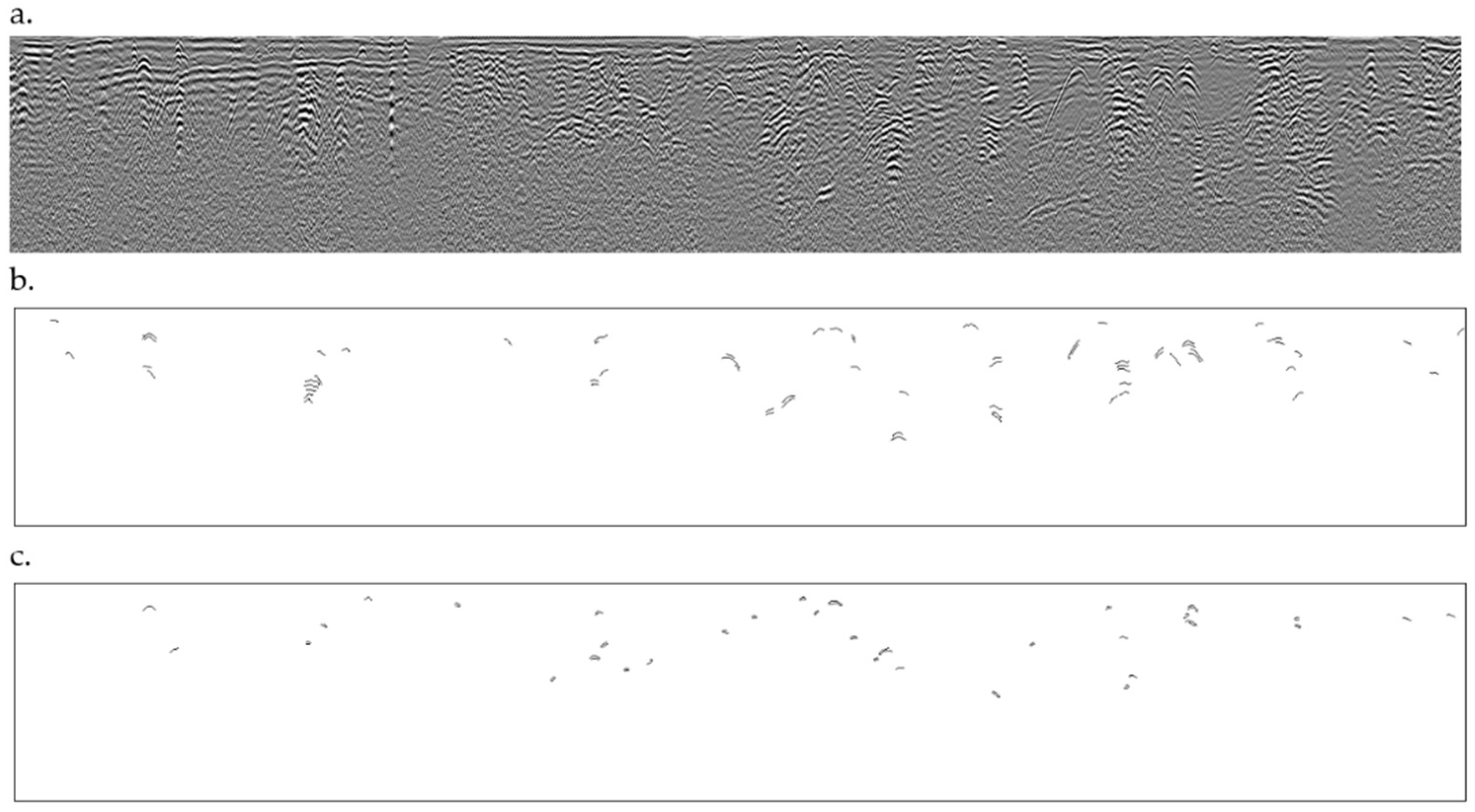
Figure 14.
Visualization of the results and showing the differences between proposed methods: (a) original GPR image; (b) hyperbolas detection result obtained from Method 1; (c) hyperbolas detection result obtained from Method 2.
Figure 14.
Visualization of the results and showing the differences between proposed methods: (a) original GPR image; (b) hyperbolas detection result obtained from Method 1; (c) hyperbolas detection result obtained from Method 2.

Figure 15.
Compliance results of classification groups: (a,c,e) comparison of the results from Method 1 and manual detection; (b,d,f) comparison of the results from Method 2 and manual detection.
Figure 15.
Compliance results of classification groups: (a,c,e) comparison of the results from Method 1 and manual detection; (b,d,f) comparison of the results from Method 2 and manual detection.

Table 1.
Technical parameters of the DS2000 Leica ground-penetrating radar [30].
Table 1.
Technical parameters of the DS2000 Leica ground-penetrating radar [30].
| Feature | Specifications |
|---|---|
| Antenna central frequencies | 250 MHz and 700 MHz |
| Sampling frequency | 400 kHz |
| Antenna orientation | Perpendicular, broadside |
| Depth detection | Up to 10 m |
| Scan interval | 42 scans/meter |
| Scan rate per channel for 512 samples/scan | 381 scans/second |
| Antenna footprint | 0.4–0.5 m |
| Acquisition speed | More than 10 km/h |
| Positioning | 2 integrated encoders—GPS and/or TPS |
Table 2.
Minimum depths of installing underground networks.
| Type of Underground Network | Minimum Depth (m) |
|---|---|
| separate telecommunication duct systems | 0.5 |
| mains telecommunication duct systems and in-ground cables | 0.7 |
| power supply cables up to 1 KV and over 1 KV | 0.7–1.0 |
| lighting cables | 0.5 |
| remotely controlled heating ducts starting from the manhole cover | 0.5 |
| gas networks | 1.0–1.2 |
| water supply networks (depending on pipe diameter) | 1.4–1.8 |
| sewers—the depth is calculated so as to maintain the proper inclination of these points | 1.4 |
Table 3.
Matrix of comparisons between the analyzed attributes.
| Attribute | Curvature | Size | Depth | ||
|---|---|---|---|---|---|
| Curvature | 1 | 5 | 5 | ||
| Size | 3 | 1 | 1 | ||
| Depth | 3 | 1 | 1 | ||
Table 4.
Measures of significance.
| Degree of Significance | Definitions |
|---|---|
| 1 | Equally important |
| 3 | Weak significance of one factor in comparison to another |
| 5 | Strong or essential importance |
Table 5.
Effectiveness of the detection of candidate objects after the introduction of conditions.
| Serial Number | 4 | 4 | 4 | 2 | 2 | 2 | 1 | 1 | 1 | 3 |
| Route Number | 3 | 6 | 11 | 3 | 6 | 11 | 3 | 6 | 11 | 3 |
| Effectiveness—Method 1 | 100% | 100% | 100% | 100% | 100% | 100% | 89% | 100% | 100% | 100% |
| SNR—Method 1 | 0.11 | 0.06 | 0.08 | 0.14 | 0.08 | 0.13 | 0.12 | 0.09 | 0.06 | 0.12 |
| Effectiveness—Method 2 | 87% | 100% | 100% | 82% | 100% | 90% | 80% | 83% | 83% | 80% |
| SNR—Method 2 | 0.25 | 0.14 | 0.21 | 0.27 | 0.16 | 0.50 | 0.25 | 0.17 | 0.18 | 0.36 |
Table 6.
Obtained average values of the parameter.
| Coefficient | Automatic Detection | |
|---|---|---|
| Method 1 | Method 2 | |
| M | 79% | 91% |
Table 7.
Obtained average values of the parameter.
| Coefficient | Automatic Detection | |
|---|---|---|
| Method 1 | Method 2 | |
| L | 6% | 13% |
Table 8.
Average values of the obtained parameters , and .
| Coefficient | Manual Detection | Automatic Detection | |
|---|---|---|---|
| Method 1 | Method 2 | ||
| 0.63 | 0.06 | 0.14 | |
| 0.88 | 0.98 | 0.86 | |
| 0.72 | 0.12 | 0.24 | |
Table 9.
Normalized matrix.
| Attribute | Weight (wc) | |||
|---|---|---|---|---|
| 0.14 | 0.71 | 0.71 | 0.52 | |
| 0.43 | 0.14 | 0.14 | 0.24 | |
| 0.43 | 0.14 | 0.14 | 0.24 |
Table 10.
Average values of the effectiveness of classification of hyperbolas and .
| Effectiveness of Classification | Group of the Classified Object | ||
|---|---|---|---|
| Certain Object | Uncertain Object | The Least Certain Objects | |
| 58% (G1 vs. G1′) | 39% (G2 vs. G2′) | 48% (G3 vs. G3′) | |
| 60% (G1 vs. G1″) | 38% (G2 vs. G2″) | 40% (G3 vs. G3″) | |
Publisher’s Note: MDPI stays neutral with regard to jurisdictional claims in published maps and institutional affiliations. |
© 2021 by the authors. Licensee MDPI, Basel, Switzerland. This article is an open access article distributed under the terms and conditions of the Creative Commons Attribution (CC BY) license (https://creativecommons.org/licenses/by/4.0/).
Share and Cite
MDPI and ACS Style
Onyszko, K.; Fryśkowska-Skibniewska, A. A New Methodology for the Detection and Extraction of Hyperbolas in GPR Images. Remote Sens. 2021, 13, 4892. https://0-doi-org.brum.beds.ac.uk/10.3390/rs13234892
AMA Style
Onyszko K, Fryśkowska-Skibniewska A. A New Methodology for the Detection and Extraction of Hyperbolas in GPR Images. Remote Sensing. 2021; 13(23):4892. https://0-doi-org.brum.beds.ac.uk/10.3390/rs13234892
Chicago/Turabian StyleOnyszko, Klaudia, and Anna Fryśkowska-Skibniewska. 2021. "A New Methodology for the Detection and Extraction of Hyperbolas in GPR Images" Remote Sensing 13, no. 23: 4892. https://0-doi-org.brum.beds.ac.uk/10.3390/rs13234892
Note that from the first issue of 2016, this journal uses article numbers instead of page numbers. See further details here.