
Local Freeman Decomposition for Robust Imaging and Identification of Subsurface Anomalies Using Misaligned Full-Polarimetric GPR Data


Abstract
:1. Introduction
2. Local Freeman Decomposition
- Only one parameter (the smoothing radius k) needs to be specified, as opposed to several (window size, overlap, and taper) in the sliding-window approach. The smoothing radius directly reflects the locality of the measurement;
- The shaping regularization method continues the measurement smoothly through the regions of absent information. This effect is impossible to achieve in the sliding-window approach unless the window size is always larger than the information gaps in the signal.
3. Results
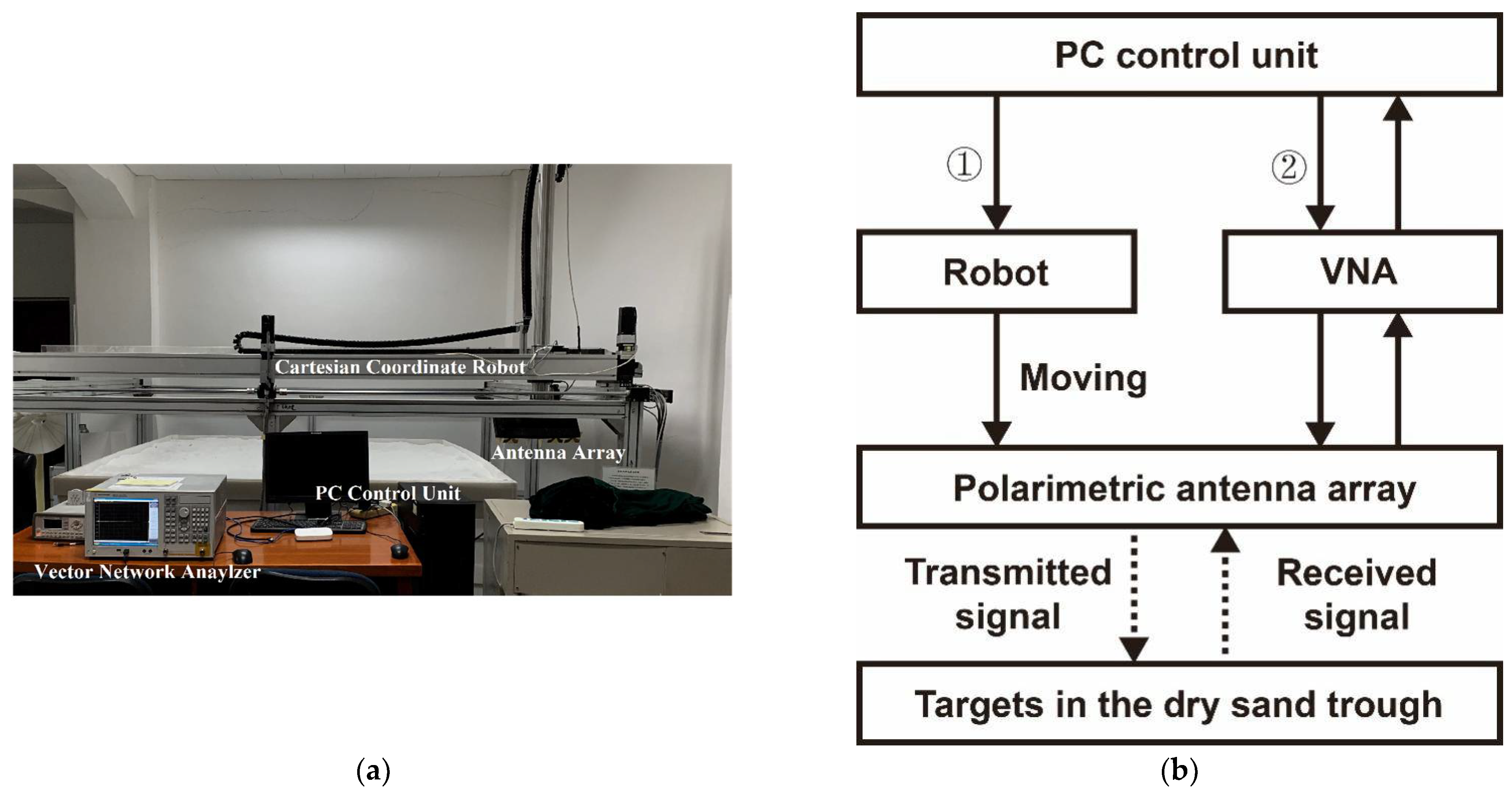
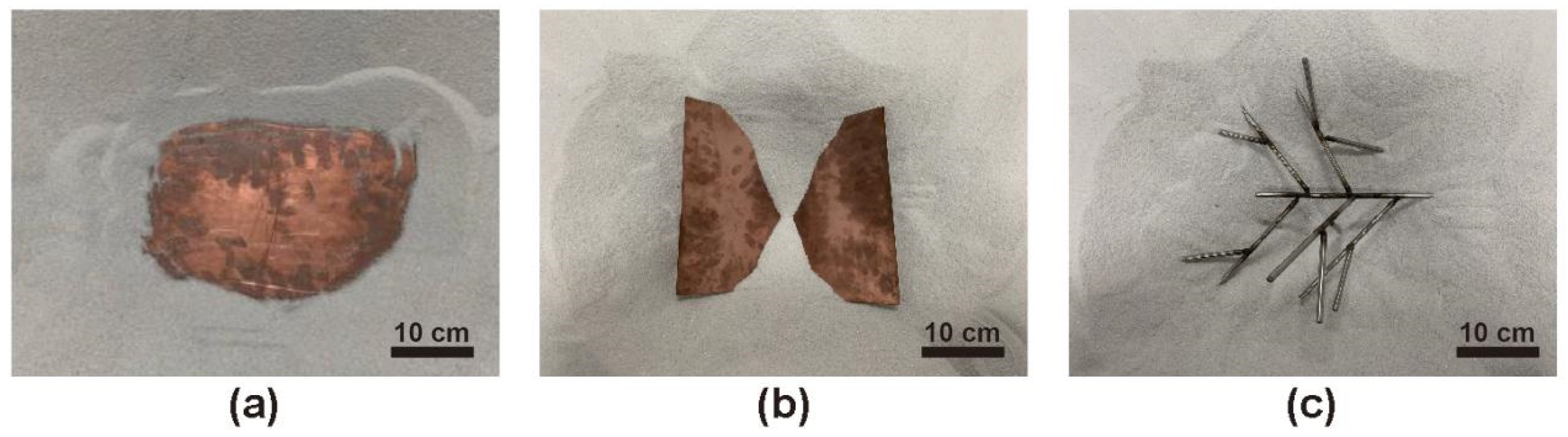
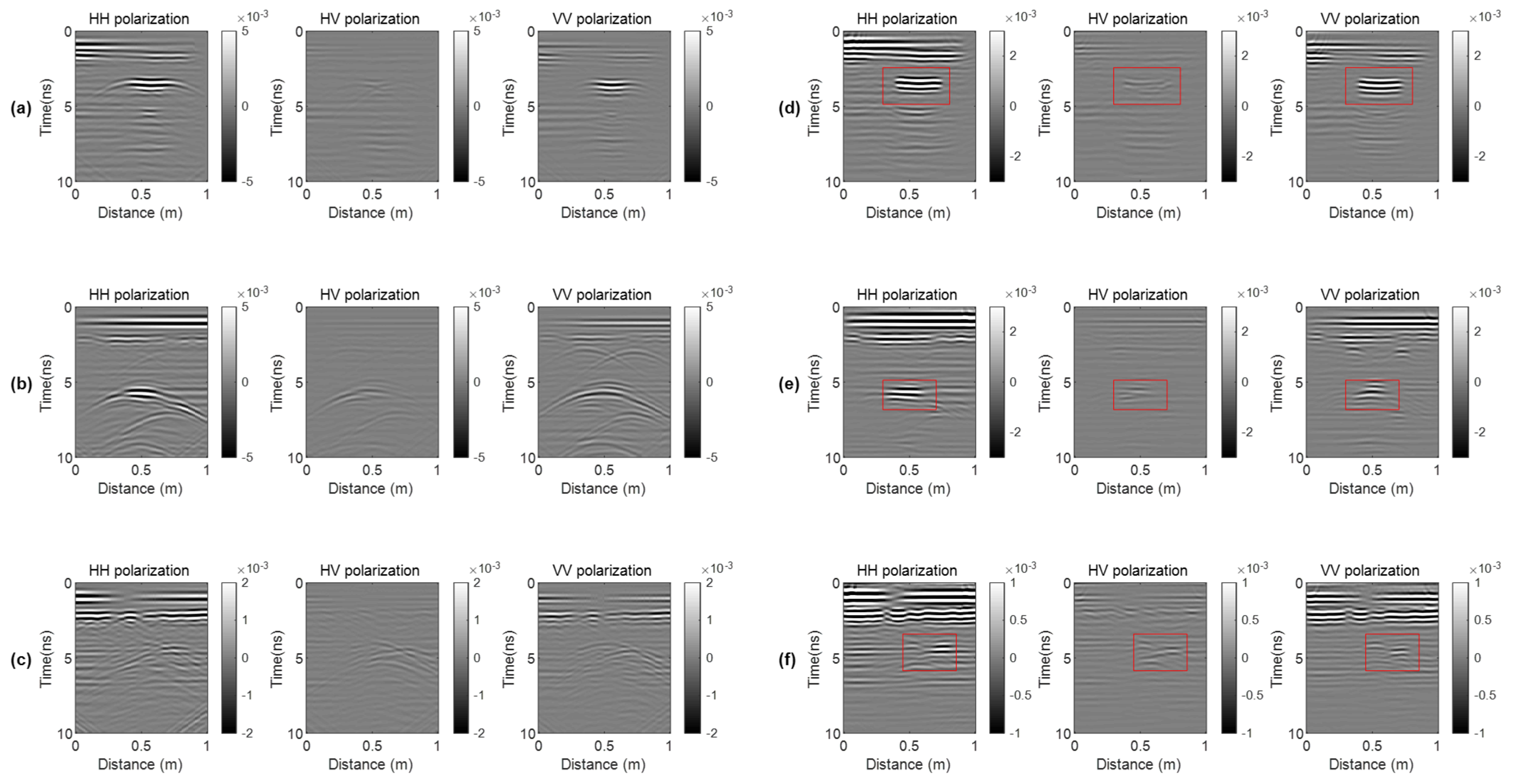
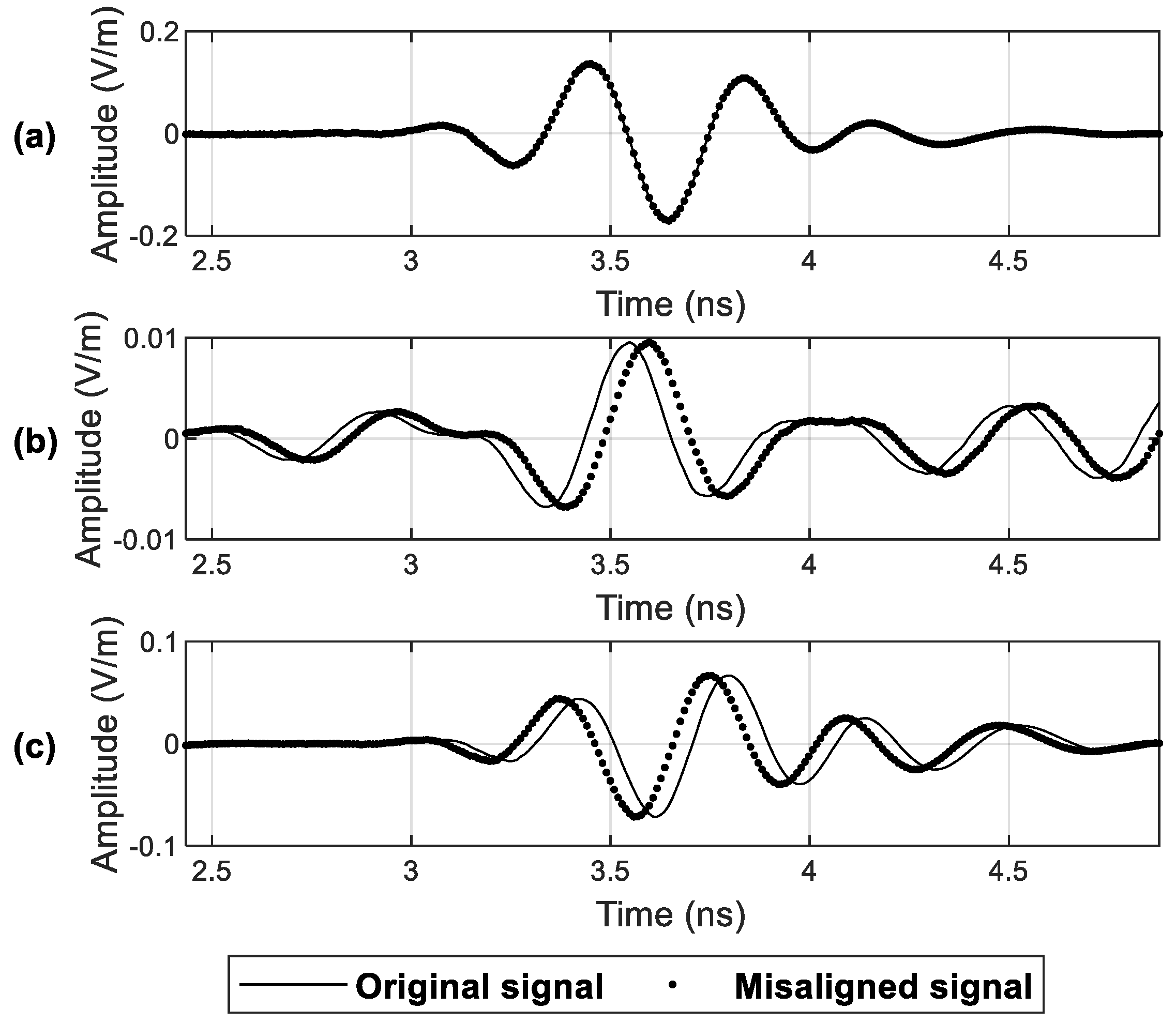
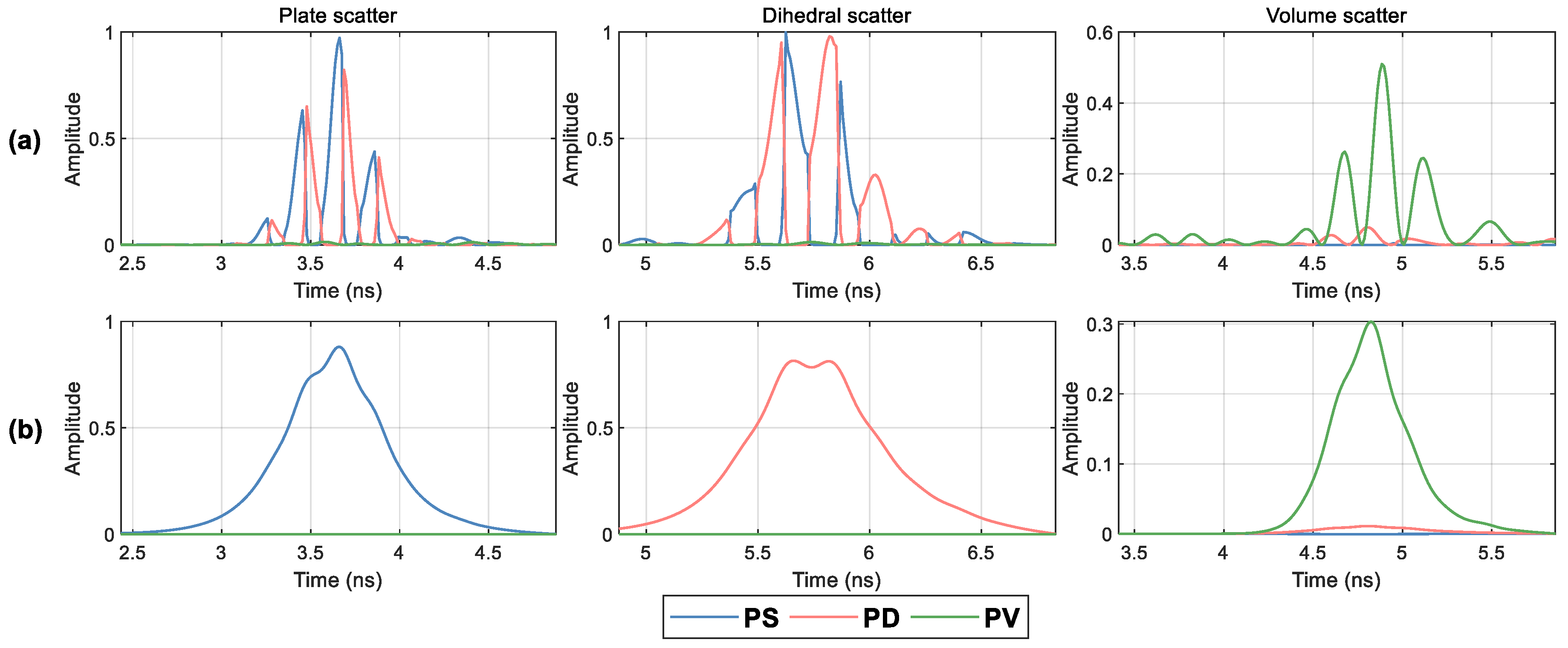
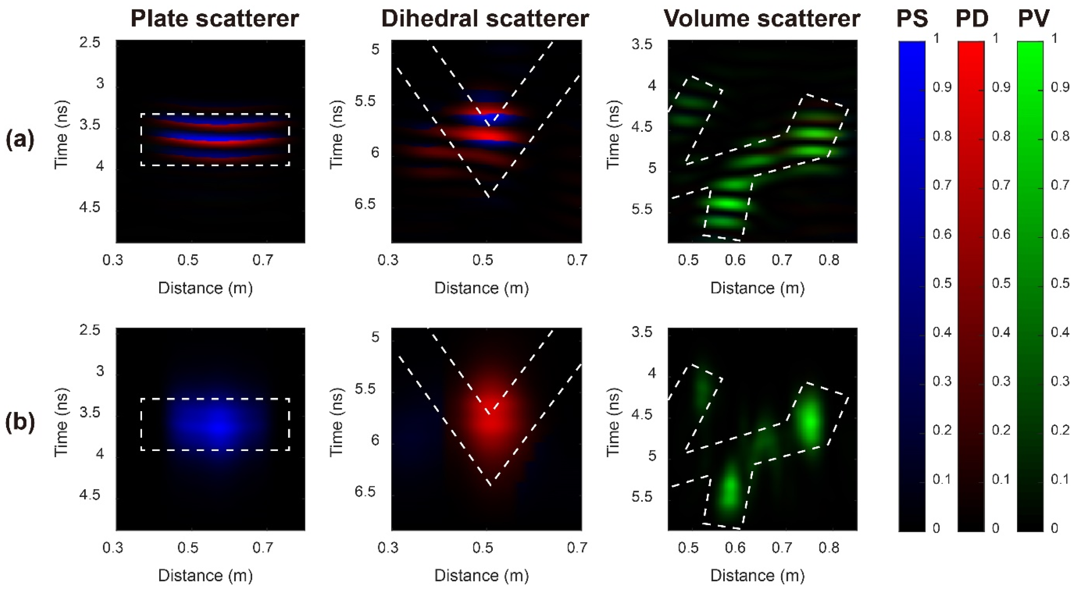
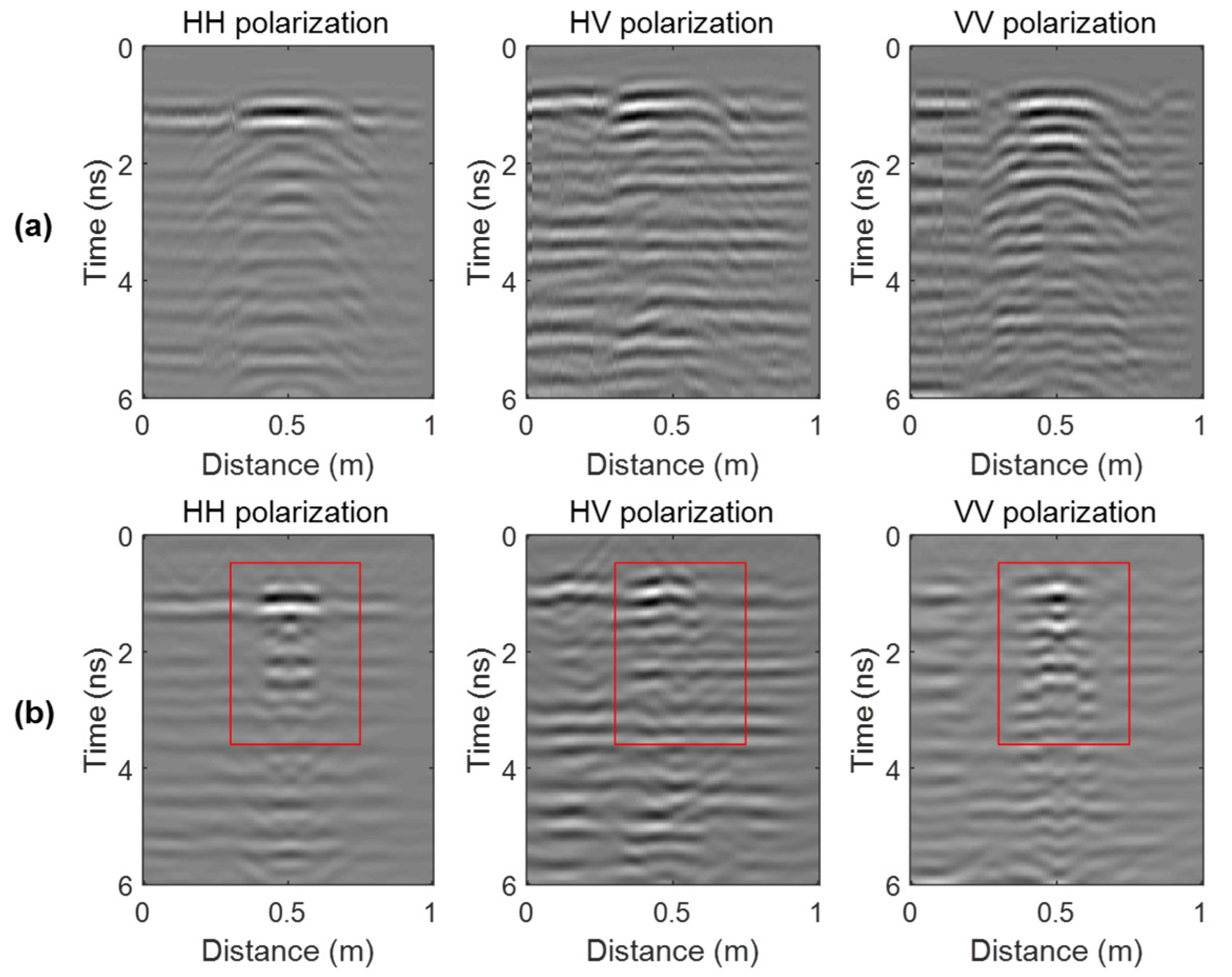
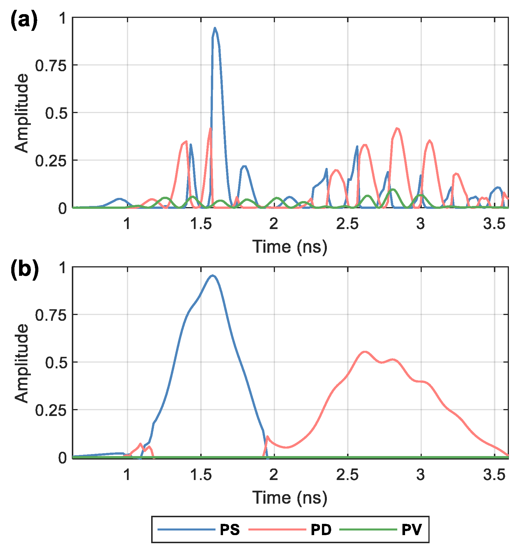
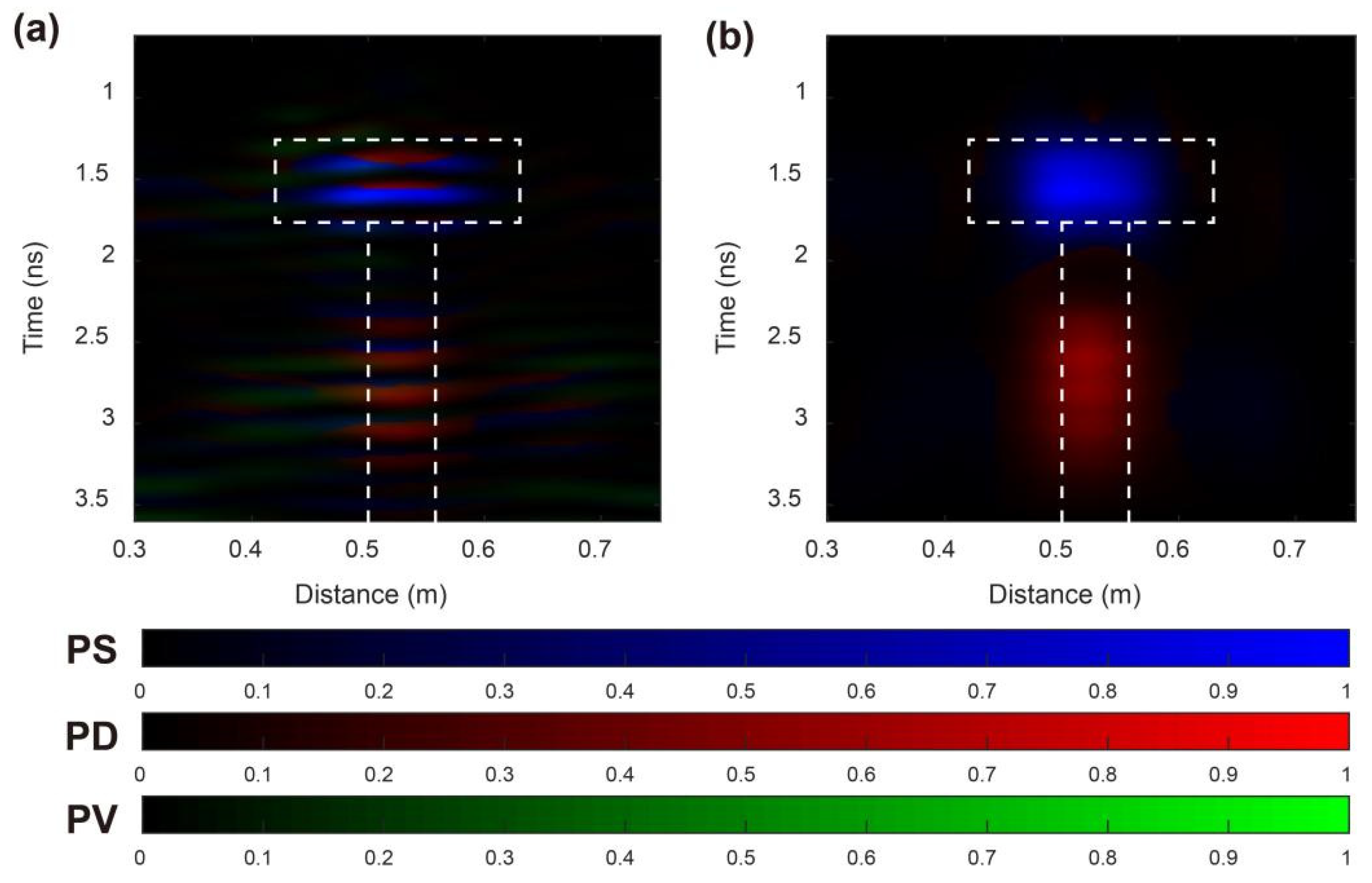
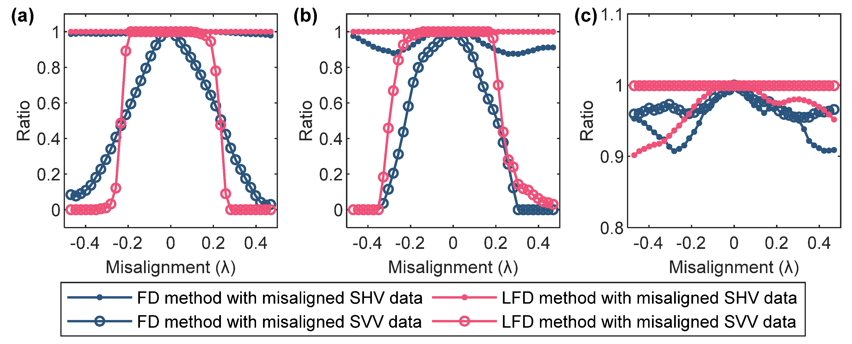
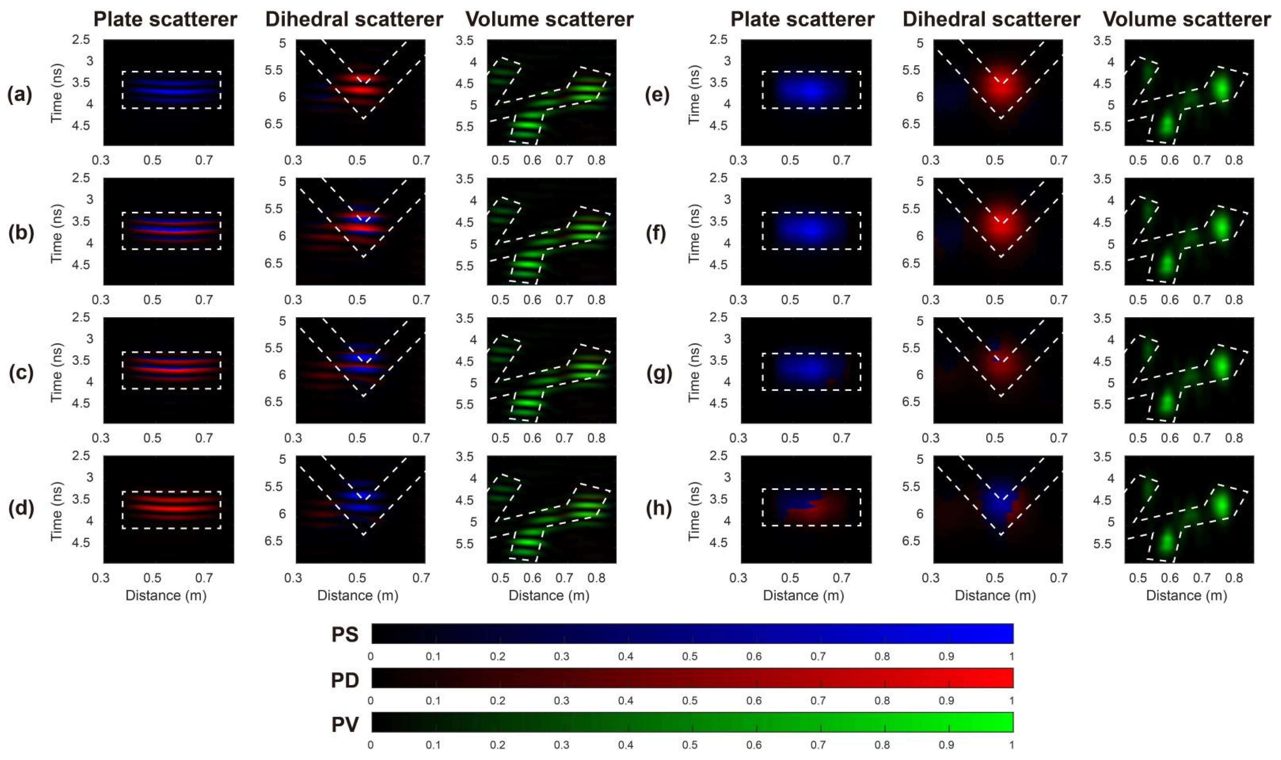
3.1. LFD Test for Misaligned FP-GPR Data of Typical Targets
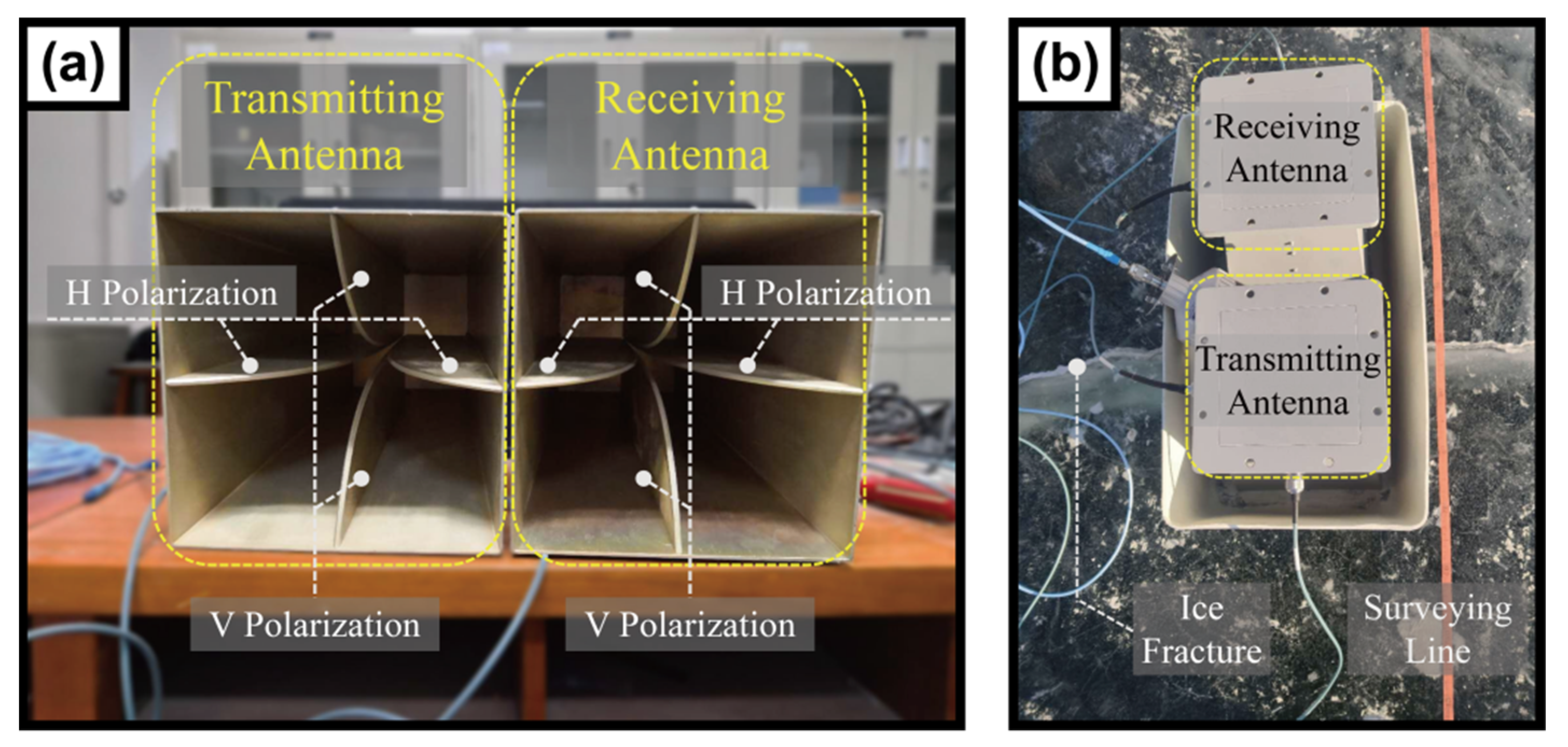
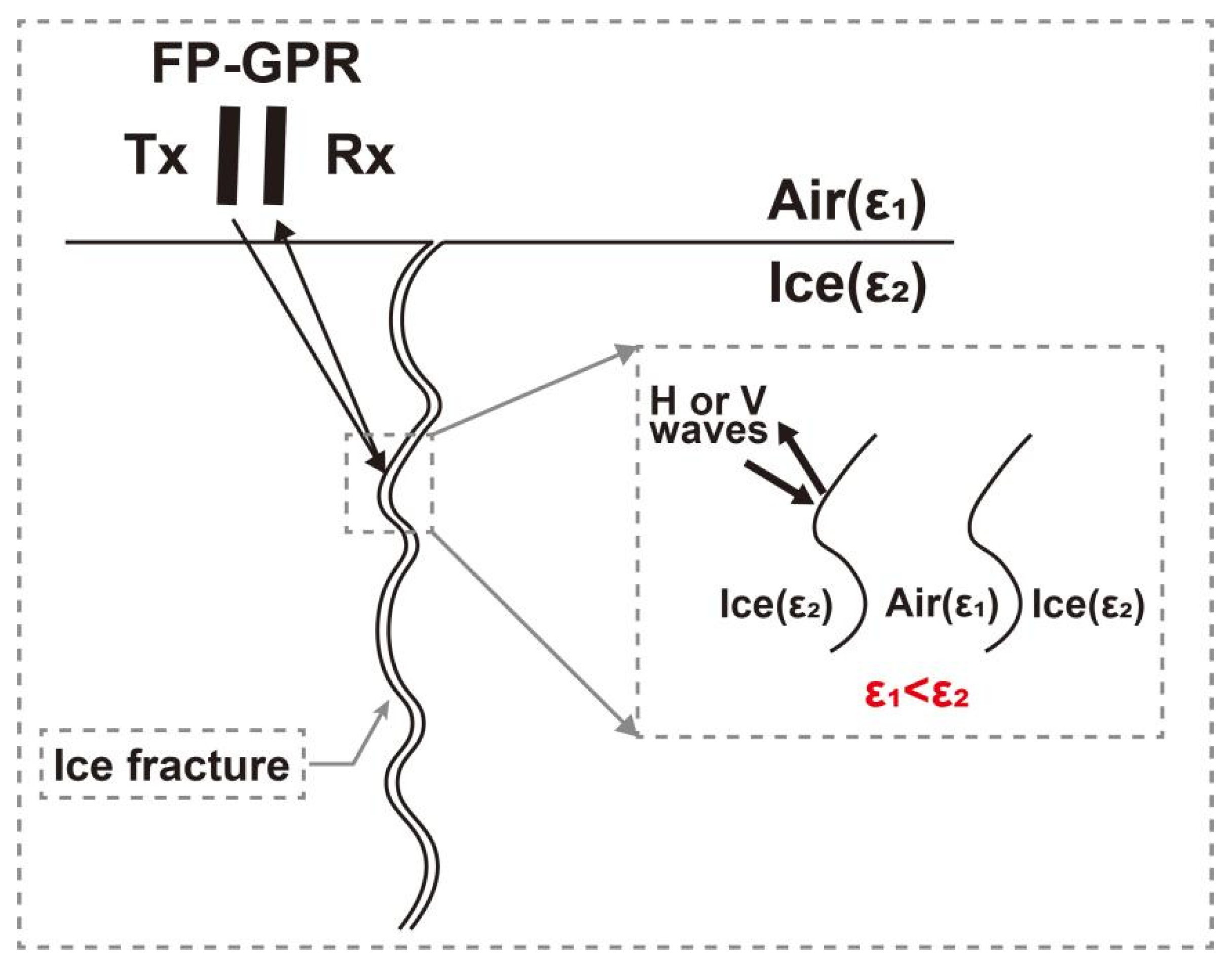
3.2. Field Application in Ice Fracture Detection
4. Discussion
5. Conclusions
Author Contributions
Funding
Data Availability Statement
Conflicts of Interest
Appendix A

| Terms | Explanations |
|---|---|
| FP-GPR | Full-polarimetric ground penetrating radar |
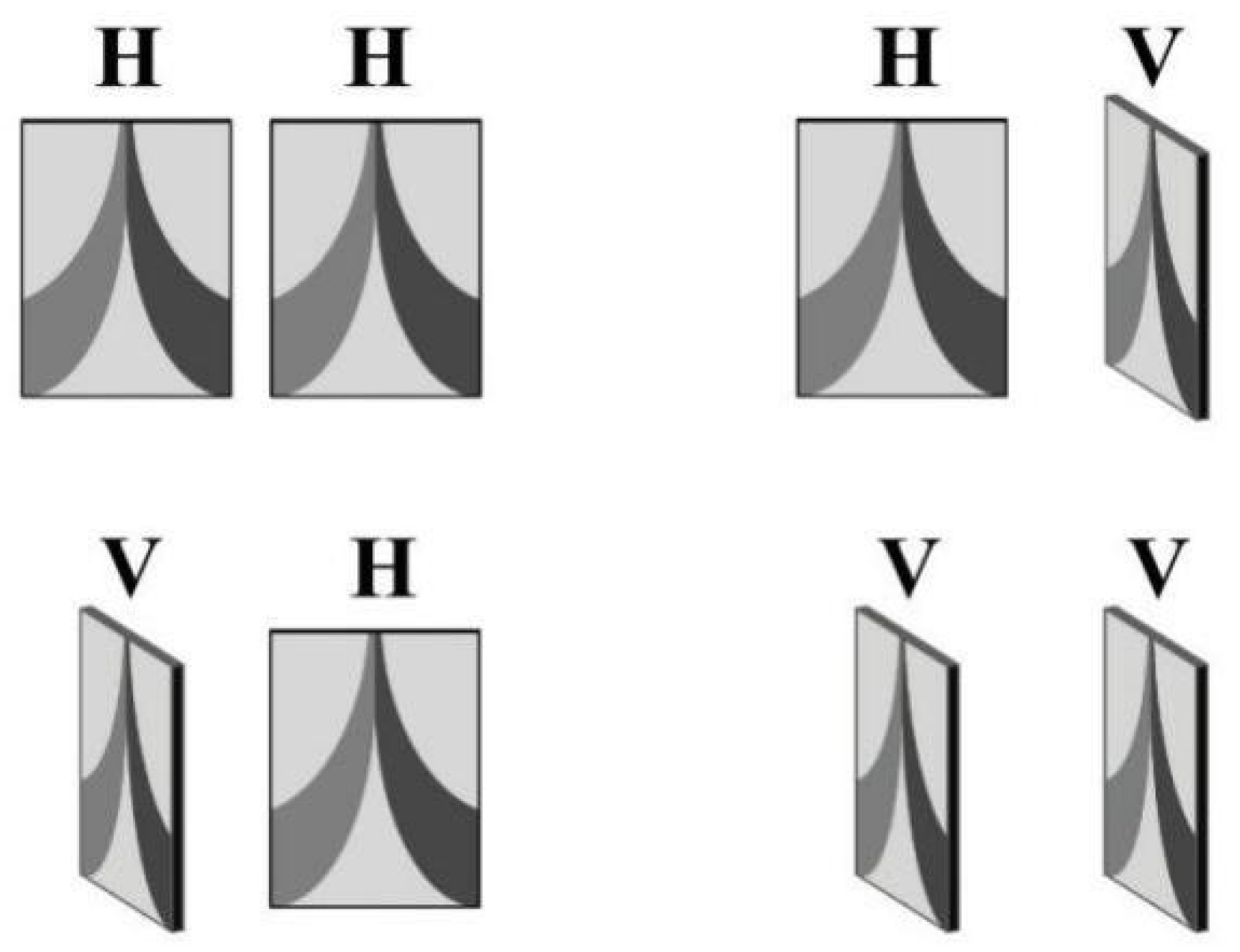
| H polarization | Horizontal polarization, the electric vector is parallel to the patrolling direction of GPR. |
| V polarization | Vertical polarization, the electric vector is vertical to the patrolling direction of GPR. |
| Sinclair matrix | A matrix composes of four types of data in radar polarimetry. |
| Target decomposition | Analyzing the characteristics of a Sinclair matrix. mathematically or physically and obtain the polarization properties of a target. |
| Target vector | The vector form of a Sinclair matrix. |
| Straightforward lexicographic ordering | Decomposing a Sinclair matrix into a target vector using the lexicographic basis: |
| Span (total power) | |
| Target covariance matrix | A matrix generated by multiplying a target vector and its conjugate transpose. |
References
- Feng, X.; Sato, M. Pre-stack migration applied to GPR for landmine detection. Inverse Prob. 2004, 20, 99–115. [Google Scholar] [CrossRef]
- Sassen, D.S.; Everett, M.E. 3D polarimetric GPR coherency attributes and full-waveform inversion of transmission data for characterizing fractured rock. Geophysics 2009, 74, J23–J34. [Google Scholar] [CrossRef]
- Böniger, U.; Tronicke, J. Subsurface Utility Extraction and Characterization: Combining GPR Symmetry and Polarization Attributes. IEEE Trans. Geosci. Remote Sens. 2011, 50, 736–746. [Google Scholar] [CrossRef]
- Allred, B.J.; Daniels, J.J.; Fausey, N.R.; Chen, C.C.; Peters, L., Jr.; Youn, H.S. Important Considerations for Locating Buried Agricultural Drainage Pipe Using Ground Penetrating Radar. J. Appl. Eng. Agric. 2005, 21, 71–87. [Google Scholar] [CrossRef]
- O’Neill, K. Discrimination of UXO in Soil Using Broadband Polarimetric GPR Backscatter. IEEE Trans. Geosci. Remote Sens. 2001, 39, 356–367. [Google Scholar] [CrossRef]
- Tsoflias, G.P.; VanGestel, J.P.; Stoffa, P.L.; Blankenship, D.D.; Sen, M. Vertical fracture detection by exploiting the polarization properties of ground-penetrating radar signals. Geophysics 2004, 69, 803–810. [Google Scholar] [CrossRef]
- Tsoflias, G.P.; Hoch, A. Investigating multi-polarization GPR wave transmission through thin layers: Implications for vertical fracture characterization. Geophys. Res. Lett. 2006, 33, L20401. [Google Scholar] [CrossRef] [Green Version]
- Dong, Z.; Feng, X.; Zhou, H.; Liu, C.; Sato, M. Effects of Induced Field Rotation from Rough Surface on H-Alpha Decomposition of Full-Polarimetric GPR. IEEE Trans. Geosci. Remote Sens. 2021, 59, 9192–9208. [Google Scholar] [CrossRef]
- Dong, Z.; Feng, X.; Zhou, H.; Liu, C.; Sato, M. Assessing the Effects of Induced Field Rotation on Water Ice Detection of Tianwen-1 Full-Polarimetric Mars Rover Penetrating Radar. IEEE Trans. Geosci. Remote Sens. 2021. [Google Scholar] [CrossRef]
- O’Neill, K.; Haider, S.A.; Shireen, D.G.; Paulsen, K.D. Effects of the Ground Surface on Polarimetric Features of Broadband Radar Scattering from Subsurface Metallic Objects. IEEE Trans. Geosci. Remote Sens. 2001, 39, 1556–1565. [Google Scholar] [CrossRef]
- Cloude, S.R.; Pottier, E. A review of target decomposition theorems in radar polarimetry. IEEE Trans. Geosci. Remote Sens. 1996, 34, 498–518. [Google Scholar] [CrossRef]
- Chen, C.C.; Higgins, M.B.; O’Neill, K.; Detsch, R. Ultrawidebandwidth fully-polarimetric ground penetrating radar classification of subsurface unexploded ordnance. IEEE Trans. Geosci. Remote Sens. 2001, 39, 1221–1230. [Google Scholar] [CrossRef]
- Miwa, T.; Sato, M.; Niitsuma, H. Subsurface fracture measurement with polarimetric borehole radar. IEEE Trans. Geosci. Remote Sens. 1999, 37, 828–837. [Google Scholar] [CrossRef]
- Roth, F.; van Genderen, P.; Verhaegen, M. Processing and analysis of polarimetric ground penetrating radar landmine signatures. In Proceedings of the 2nd International Workshop on Advanced GPR, Delft, The Netherlands, 14–16 May 2003; pp. 14–16. [Google Scholar]
- Liu, H.; Huang, X.; Han, F.; Cui, J.; Spencer, B.F.; Xie, X. Hybrid Polarimetric GPR Calibration and Elongated Object Orientation Estimation. IEEE J. Sel. Top. Appl. Earth Observ. Remote Sens. 2019, 12, 2080–2087. [Google Scholar] [CrossRef]
- Cloude, S.R.; Pottier, E. An entropy based classification scheme for land applications of polarimetric SAR. IEEE Trans. Geosci. Remote Sens. 1997, 35, 68–78. [Google Scholar] [CrossRef]
- Yu, Y.; Chen, C.C.; Feng, X.; Liu, C. Modified Entropy-Based Fully Polarimetric Target Classification Method for Ground Penetrating Radars (GPR). IEEE J. Sel. Top. Appl. Earth Observ. Remote Sens. 2017, 10, 4304–4312. [Google Scholar] [CrossRef]
- Yu, Y.; Chen, C.C. Full-Polarization Target Classification Using Single-Polarization Ground Penetrating Radars. IEEE Trans. Geosci. Remote Sens. 2021, 60, 4504508. [Google Scholar] [CrossRef]
- Zhao, J.G.; Sato, M. Radar polarimetry analysis applied to single-hole fully polarimetric borehole radar. IEEE Trans. Geosci. Remote Sens. 2006, 44, 3547–3554. [Google Scholar] [CrossRef]
- Feng, X.; Yu, Y.; Liu, C.; Fehler, M. Combination of H-Alpha Decomposition and Migration for Enhancing Subsurface Target Classification of GPR. IEEE Trans. Geosci. Remote Sens. 2015, 53, 4852–4861. [Google Scholar] [CrossRef]
- Feng, X.; Yu, Y.; Liu, C.; Fehler, M. Subsurface polarimetric migration imaging for full polarimetric ground-penetrating radar. Geophys. J. Int. 2015, 202, 1324–1338. [Google Scholar] [CrossRef] [Green Version]
- Zhou, H.; Feng, X.; Zhang, Y.; Nilot, E.; Zhang, M.; Dong, Z.; Qi, J. Combination of Support Vector Machine and H-Alpha Decomposition for Subsurface Target Classification of GPR. In Proceedings of the 17th International Conference on Ground Penetrating Radar (GPR), Rapperswil, Switzerland, 18–21 June 2018; pp. 635–638. [Google Scholar]
- Feng, X.; Zhou, H.; Liu, C.; Zhang, Y.; Liang, W.; Nilot, E.; Zhang, M.; Dong, Z. Particle center supported plane for subsurface target classification based on full polarimetric ground penetrating radar. Remote Sens. 2019, 11, 405. [Google Scholar] [CrossRef] [Green Version]
- Liu, H.; Zhong, J.; Ding, F.; Meng, X.; Liu, C.; Cui, J. Detection of Early-stage Rebar Corrosion Using a Polarimetric Ground Penetrating Radar System. Constr. Build. Mater. 2022, 317, 1–10. [Google Scholar] [CrossRef]
- Freeman, A.; Durden, S.L. A three-component scattering model for polarimetric SAR Data. IEEE Trans. Geosci. Remote Sens. 1998, 36, 963–973. [Google Scholar] [CrossRef] [Green Version]
- Zhao, J.; Sato, M. Consistency Analysis of Subsurface Fracture Characterization Using Different Polarimetry Techniques by a Borehole Radar. IEEE Geosci. Remote Sens. Lett. 2007, 4, 359–363. [Google Scholar] [CrossRef]
- Feng, X.; Liang, W.J.; Liu, C.; Nilot, E.; Zhang, M.; Liang, S. Application of Freeman decomposition to full polarimetric GPR for improving subsurface target classification. Signal Process. 2017, 132, 284–292. [Google Scholar] [CrossRef]
- Fomel, S. Shaping regularization in geophysical-estimation problems. Geophysics 2007, 72, R29–R36. [Google Scholar] [CrossRef]
- Fomel, S. Local Seismic Attributes. Geophysics 2007, 72, A29–A33. [Google Scholar] [CrossRef]
- van Zyl, J.J.; Zebker, H.A.; Elachi, C. Imaging radar polarization signatures: Theory and observation. Radio Sci. 1987, 22, 529–543. [Google Scholar] [CrossRef]
- Boerner, W.M.; Mott, H.; Lfineburg, L.; Livingstone, C.; Pottier, E. Polarimetry in radar remote sensing: Basic and applied concepts. In Principles and Applications of Imaging Radar, The Manual of Remote Sensing, 3rd ed.; Wiley: New York, NY, USA, 1998; Volume 2. [Google Scholar]
- Ziegler, V.; Luneburg, E.; Schroth, A. Mean Backscattering Properties of Random Radar Targets: A Polarimetric Covariance Matrix Concept. In Proceedings of the IGARSS ’92, 12th Annual International Geoscience and Remote Sensing Symposium, Houston, TX, USA, 26–29 May 1992; pp. 266–268. [Google Scholar]
- van Zyl, J.J. Unsupervised Classification of Scattering Behavior Using Radar Polarimetry Data. IEEE Trans. Geosci. Remote Sens. 1989, 27, 36–45. [Google Scholar] [CrossRef]
- Ulaby, F.T.; Held, D.; Dobson, M.C.; McDonald, K.C.; Senior, T.B.A. Relating Polaization Phase Difference of SAR Signals to Scene Properties. IEEE Trans. Geosci. Remote Sens. 1987, GE-25, 83–92. [Google Scholar] [CrossRef]
- Cloude, S.R. Polarisation Applications in Remote Sensing; Oxford University Press: New York, NY, USA, 2010. [Google Scholar]


Publisher’s Note: MDPI stays neutral with regard to jurisdictional claims in published maps and institutional affiliations. |
© 2022 by the authors. Licensee MDPI, Basel, Switzerland. This article is an open access article distributed under the terms and conditions of the Creative Commons Attribution (CC BY) license (https://creativecommons.org/licenses/by/4.0/).
Share and Cite
Zhou, H.; Feng, X.; Dong, Z.; Liu, C.; Liang, W.; An, Y. Local Freeman Decomposition for Robust Imaging and Identification of Subsurface Anomalies Using Misaligned Full-Polarimetric GPR Data. Remote Sens. 2022, 14, 804. https://0-doi-org.brum.beds.ac.uk/10.3390/rs14030804
Zhou H, Feng X, Dong Z, Liu C, Liang W, An Y. Local Freeman Decomposition for Robust Imaging and Identification of Subsurface Anomalies Using Misaligned Full-Polarimetric GPR Data. Remote Sensing. 2022; 14(3):804. https://0-doi-org.brum.beds.ac.uk/10.3390/rs14030804
Chicago/Turabian StyleZhou, Haoqiu, Xuan Feng, Zejun Dong, Cai Liu, Wenjing Liang, and Yafei An. 2022. "Local Freeman Decomposition for Robust Imaging and Identification of Subsurface Anomalies Using Misaligned Full-Polarimetric GPR Data" Remote Sensing 14, no. 3: 804. https://0-doi-org.brum.beds.ac.uk/10.3390/rs14030804