Article

Performance Analysis of Ocean Eddy Detection and Identification by L-Band Compact Polarimetric Synthetic Aperture Radar

1
Southern Marine Science and Engineering Guangdong Laboratory (Guangzhou), Guangzhou Institute of Geography, Guangdong Academy of Sciences, Guangzhou 510070, China
2
Key Lab of Guangdong for Utilization of Remote Sensing and Geographical Information System, Guangzhou Institute of Geography, Guangdong Academy of Sciences, Guangzhou 510070, China
3
Guangdong Province Engineering Laboratory for Geographic Spatio-Temporal Big Data, Guangzhou Institute of Geography, Guangdong Academy of Sciences, Guangzhou 510070, China
4
University of Chinese Academy of Sciences, Beijing 100049, China
5
Guangzhou Institute of Geochemistry, Chinese Academy of Sciences, Guangzhou 510640, China
*
Author to whom correspondence should be addressed.
Remote Sens. 2021, 13(23), 4905; https://0-doi-org.brum.beds.ac.uk/10.3390/rs13234905
Submission received: 20 October 2021 / Revised: 23 November 2021 / Accepted: 26 November 2021 / Published: 3 December 2021
(This article belongs to the Special Issue RADARSAT Constellation Mission (RCM))

Abstract

:
The automatic detection and analysis of ocean eddies has become a popular research topic in physical oceanography during the last few decades. Compact polarimetric synthetic aperture radar (CP SAR), an emerging polarimetric SAR system, can simultaneously acquire richer polarization information of the target and achieve large bandwidth observations. It has inherent advantages in ocean observation and is bound to become an ideal data source for ocean eddy observation and research. In this study, we simulated the CP data with L-band ALOS PALSAR fully polarimetric data. We assessed the detection and classification potential of ocean eddies from CP SAR by analyzing 50 CP features for 2 types of ocean eddies (“black”and “white”) based on the Euclidean distance and further carried out eddy detection and eddy information extraction experiments. The results showed that among the 50 CP features, the dihedral component power (Pd), shannon entropy (SEI), double bounce (Dbl), Stokes parameters (g0 and g3), eigenvalue (l1), lambda, RVoG parameter (ms), shannon entropy (SE), surface scattering component (Ps), and σ H H all performed better for detecting “white” eddies. Moreover, the H-A combination parameter (1mHA), entropy, shannon entropy (SEP, SEI, and SE), probability (p2), polarization degree (m), anisotropy, probability (p1), double bounce (Dbl), H-A combination parameter (H1mA), circular polarization ratio (CPR), and σ V V were better CP features for detecting “black” eddies.

1. Introduction

Ocean eddies represent an important ocean phenomenon, affecting both surface currents and the transportation of chemical substances, which play a significant role in theocean circulation structure and marine ecology. Moreover, ocean eddies also affect atmospheric phenomena, such as wind, clouds, and rainfall through air–sea interactions [1,2]. Tracking and observing eddies has become one of the most critical advances in ocean remote sensing in the 21st century. Broadly speaking, “ocean eddy” is the general term for a rotating seawater motion with a scale smaller than a Rossby wave controlled by the geostrophic potential eddy conservation equation, including the vortex, swirl, ring, meander, filament, and wake [3,4].
Since ocean eddies were first discovered in the 1970s, the observation of mesoscale eddies has primarily relied on dynamic sea surface height data obtained from satellite altimeters to retrieve and track eddies [5,6]. However, owing to the low spatial resolution of traditional satellite altimeter data, it is difficult to detect sub-mesoscale eddies and small-scale eddies ranging from 1 to 100 km, severely restricting eddies’ identification [7]. Because ocean eddies play a vital role in regulating changes in the sea surface temperature (SST) and chlorophyll concentration, high-resolution optical sensors have been used to detect sub-mesoscale and small-scale eddies by determining the SST [8,9] and ocean color (chlorophyll concentration) [10] variations. However, the SST and ocean color are affected by various oceanic phenomena in addition to eddies. Therefore, using the SST and water color data sets to detect eddies is prone to false alarms. Furthermore, optical sensors have proven to be vulnerable to illumination and cloud occlusion. In addition, considering the different types of observation platforms, it has been found that tracking buoys [11], airborne sensors [12], and other observation methods have high costs and are not suitable for large-scale observations.As an alternative, synthetic aperture radar (SAR) collects data throughout the day in all weather conditions and is not influenced by clouds, fog, or light [13]. Moreover, SAR images acquired over the sea contain extensive information on small-scale and mesoscale ocean phenomena, such as surface waves [14], internal waves [15], and ocean fronts [16]. Therefore, SAR images have become an ideal data source for monitoring ocean eddies [1,13,17,18,19,20].
Ocean eddies typically appear indirectly in SAR images, and there are two main mechanisms:
  • When there are natural tracers present on the sea surface such as sea ice, plankton, and oil spills, the resulting dampening of the capillary gravity waves and reduction of sea surface fluctuations cause weakening of the SAR backscatter. Moreover, because eddies are characterized by a significant transport capacity and material entrapment, if the tracer’s area is coupled with an eddy, the tracer will show a specific spiral distribution pattern under the influence of the eddy and appear in the SAR image. As a result, the backscattering contrast difference can reach 5–10 dB, and thus the eddy can be detected by identifying the tracer [21,22]. This effect typically results in a black-colored appearance for the eddies, which are collectively referred to as “black” eddies (B-E);
  • As a contrasting mechanism, the interaction of surface waves with converging and shearing surface currents results in a significant enhancement of the SAR backscatter, leading to a series of bright bands on the image that outline the contours of the eddies. These eddies are collectively referred to as “white” eddies (W-E) [23,24].
In recent decades, researchers have conducted numerous studies on the application of SAR in ocean eddy observation. In terms of statistical research on eddies, Andrei and Anna [2] used SAR satellite eddy data, including Almaz-1, the Earth Resources Satellite (ERS-1/2), Japanese ERS (JERS-1), and RADARSAT, to analyze the classification of typical ocean eddies statistically. They reported that SAR has significant potential for identifying and dynamically monitoring ocean eddies In another study, Svetlana et al. [24] used more than 500 ENVISAT ASAR images acquired in the Red Sea region from 2006 to 2011 to statistically analyze the temporal and spatial distribution characteristics of the sub-mesoscale, mesoscale, and large-scale ocean eddies in that sea region. Similarly, Xu et al. [20] used 426 scenes of ERS-2 and ENVISAT ASAR data from 2005 to 2011 to study the characteristics of ocean eddies in the Luzon Strait and its adjacent waters. In terms of eddy detection and feature parameter extraction, Was and Andharia [25] conducted research on the inversion of an ocean eddy’s rotation speed and vortex intensity based on SAR images, while Yang et al. [26] proposed an SAR image eddy information extraction method based on logarithmic spiral edge fitting to extract eddy information such as the center position, diameter, and edge size. Schuler et al. [27] used Cloude–Pottier polarization decomposition to obtain the entropy/anisotropy/alpha feature parameters, combined with the Wishart classifier, proposed a sea surfactant oil film detection algorithm, which was then applied to eddy identification. In accordance with the rapid development and broad application of artificial intelligence technology in recent years, Huang et al. [28] proposed a deep learning network model based on principal component analysis (PCA) filtering convolution. This deep learning model can learn the advanced and invariant features of ocean eddies in SAR images and provide automatic and accurate eddy detection without requiring expert interpretation knowledge. In addition to these studies, significant research has been conducted on eddy detection [29,30,31], the formation mechanism of ocean eddies based on SAR [32,33], and ocean eddy SAR image simulation methods [34]. In brief, current research on SAR eddies has predominately focused on the traditional polarization mode (single and dual polarimetric). Little research has been conducted on compact polarimetric (CP) SAR.
Over time, SAR has transformed from a single polarimetric system to a multi-polarimetric system with fully polarimetric (FP) observation capabilities after its 50 years of development. Compared with single-polarimetric SAR, dual-polarimetric (DP) or FP SAR can obtain more scattering characteristics of the observation target, significantly improving the detection ability [35,36,37,38]. Although its improved target detection capabilities characterize FP SAR, its image width is much smaller than that of the single polarized SAR (e.g., the FP SAR image width of RADARSAT-2 is only 25/50 km, while the image width of the single-polarimetric ScanSAR mode is 500 km). Moreover, the system structure is complex, and the maintenance cost is extremely high, which significantly limits the application of FP SAR. To overcome the shortcomings of single-polarimetric and FP SAR, CP SAR that uses a special DP SAR structure was proposed in 2005 [39,40]. This can achieve both a wide range of observations (up to 350 km) and obtain polarization scattering information close to that which can be obtained by FP SAR. In light of the unique advantages of CP SAR, Canada’s RADARSAT Constellation Missions (RCM) [41], India’s Risat-1 satellite [42], and Japan’s Advanced Land Observing Satellite 2 (ALOS-2) have all supported the CP mode and are being actively researched.
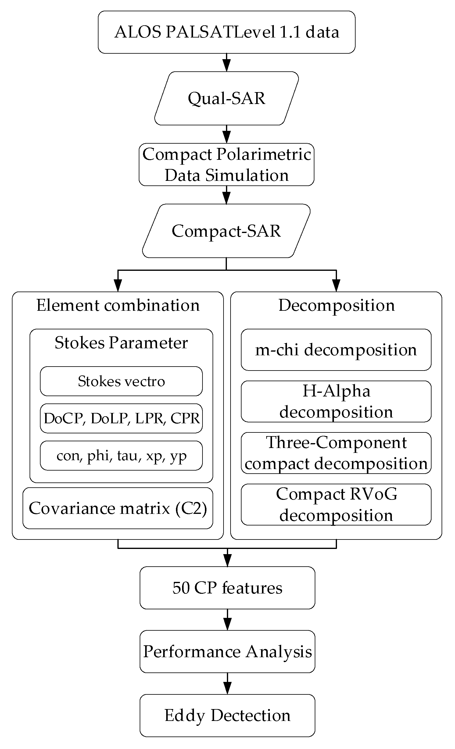
However, there is no relevant research on the use of CP SAR to observe ocean eddies. To develop CP SAR eddy detection technology, it is necessary to fully understand the response characteristics of CP SAR to ocean eddies. This study investigates the response characteristics of CP SAR to ocean eddies by extracting 50 types of CP features from 2 scenes of ALOS Phased Array type L-band SAR (PALSAR) data (the image covers the W-E and B-E) and then compares and analyzes the ocean eddy detection performance of the 50 features. On this basis, eddy detection and eddy information extraction experiments are conducted. This work contributes to developing subsequent work on CP SAR eddy detection and eddy refinement structure studies. The chapter structure of this article is as follows. Section 2 introduces the data and describes eddies. Section 3 introduces CP theory, CP data acquisition, and the feature extraction process. Section 4 conducts a comprehensive quantification and evaluation of CP features for eddy detection. Section 5 presents the eddy detection and eddy information extraction experiments. Section 6 discusses the results, and finally, the paper is concluded.

2. Data and Eddies

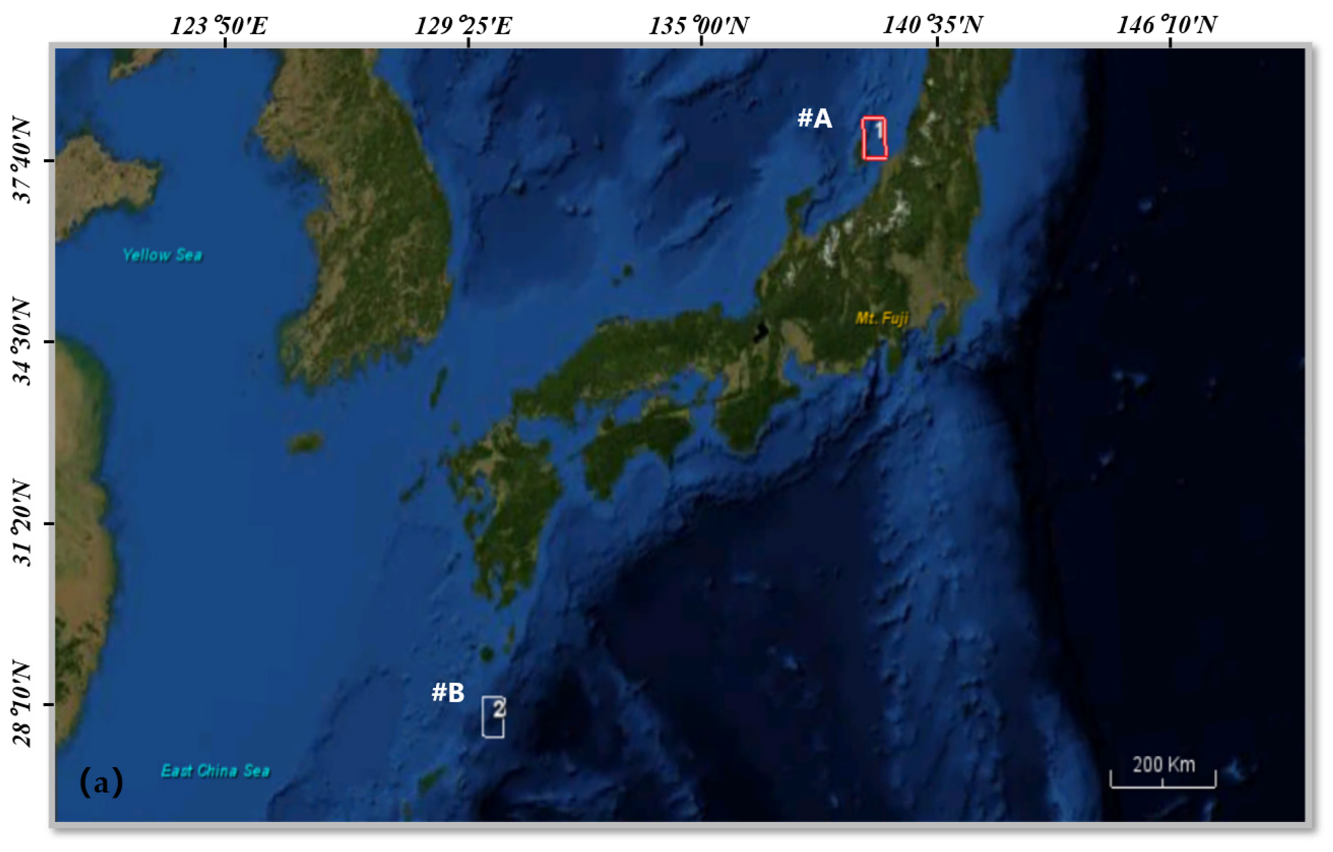
In this study, two PALSAR images were obtained (Figure 1). PALSAR is an L-band FP SAR sensor carried by the Japanese ALOS-1 satellite. The product used was a Level 1.1 single-look complex data with an azimuthal resolution of approximately 24 m and a distance resolution of approximately 10 m. Images #A and #B of the sea around Japan (Figure 2a) were acquired on 11 November 2010 at 1:00 p.m. UTC and 2 April 2011 at 1:23 p.m. UTC, respectively.
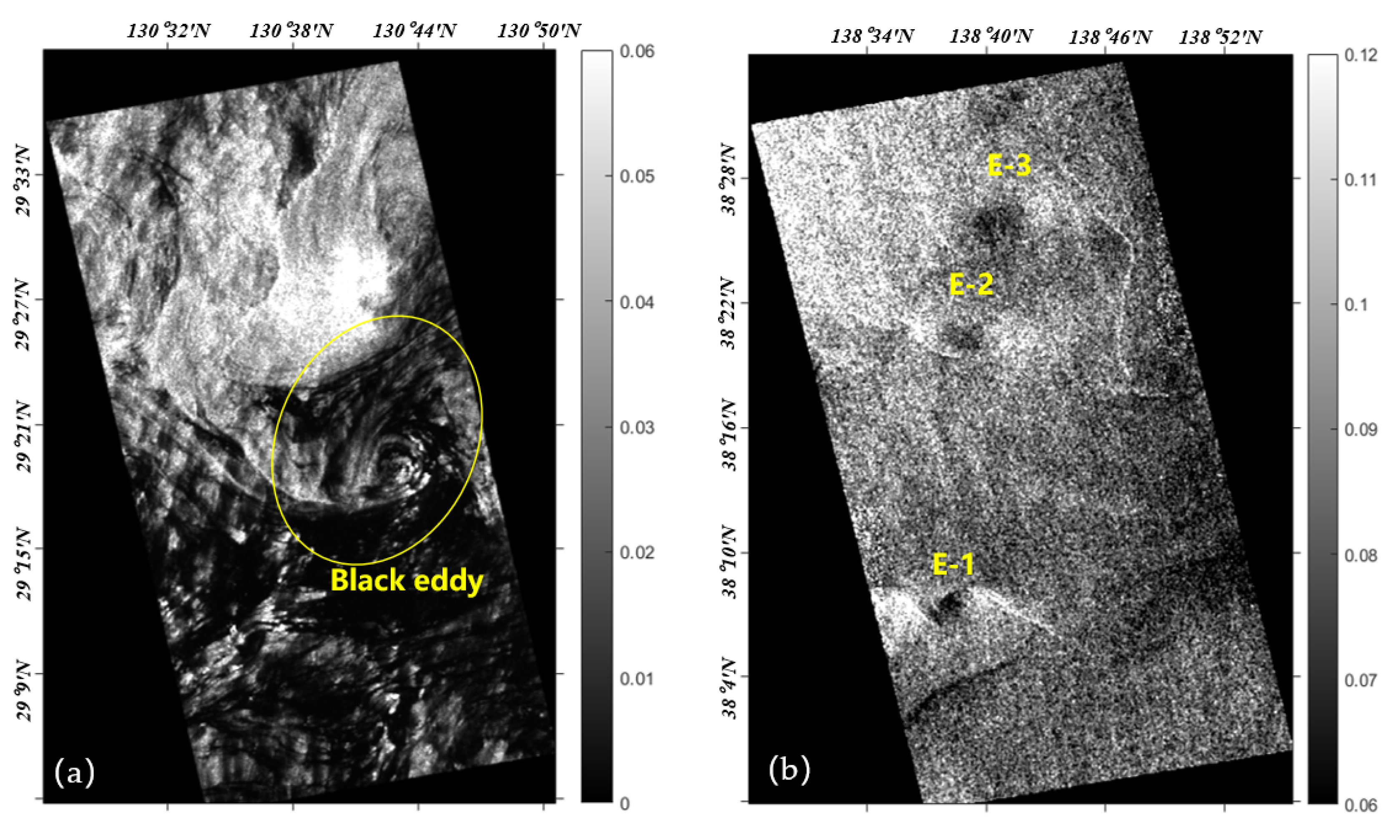
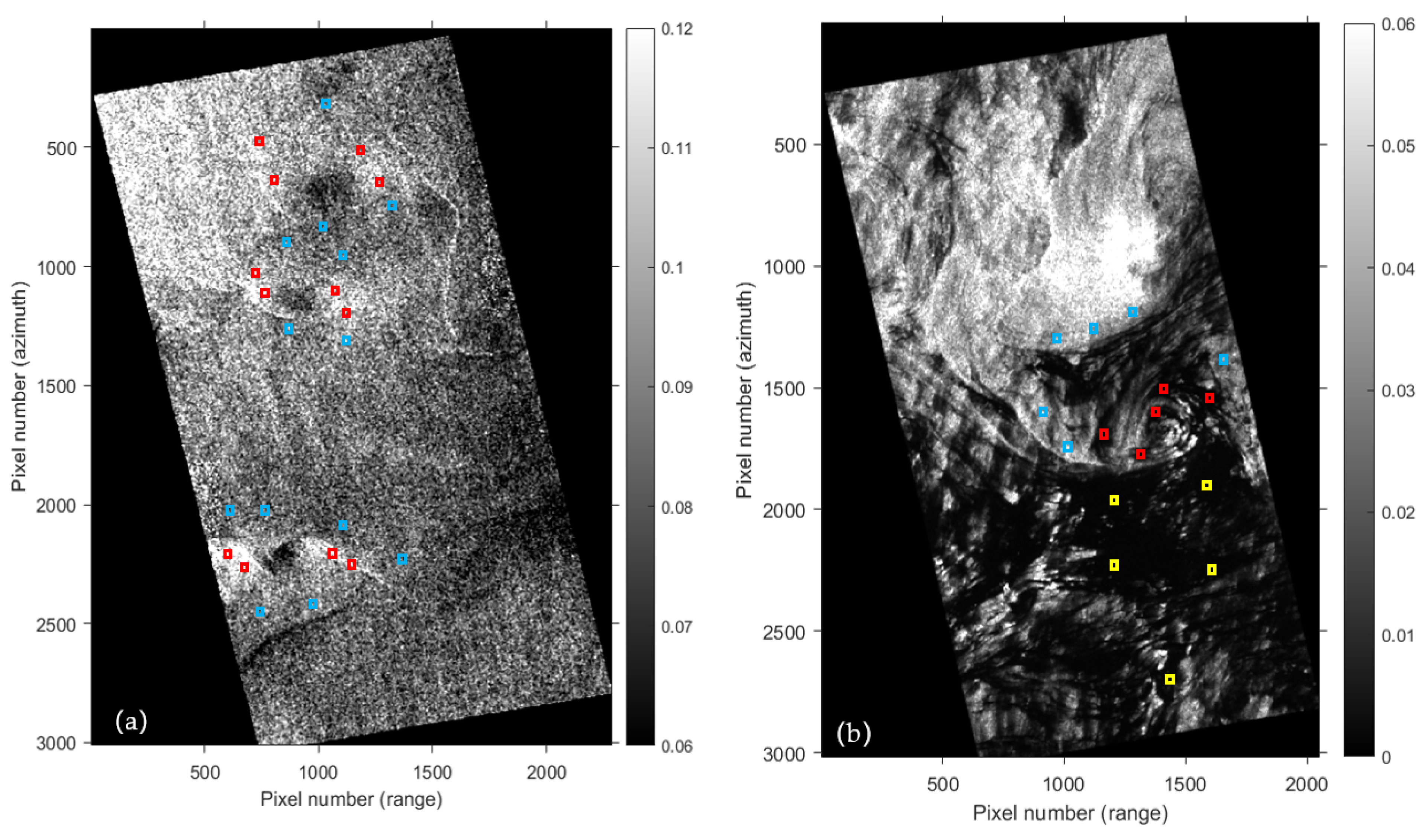
Figure 1a shows the #A VV-polarized backscatter coefficient image, which contains three suspected W-E with diameters of 12 km (E-1), 13 km (E-2), and 15 km (E-3) from bottom to top. These three regions are very similar to the W-E morphological structure that has been described in the literature [26], with dark areas in the middle and bright areas on both sides. Data #A are located on the northeast side of Sado Island, and studies have shown that small eddies usually form near the coastline or between islands due to the interaction between the coastline and surface currents [43,
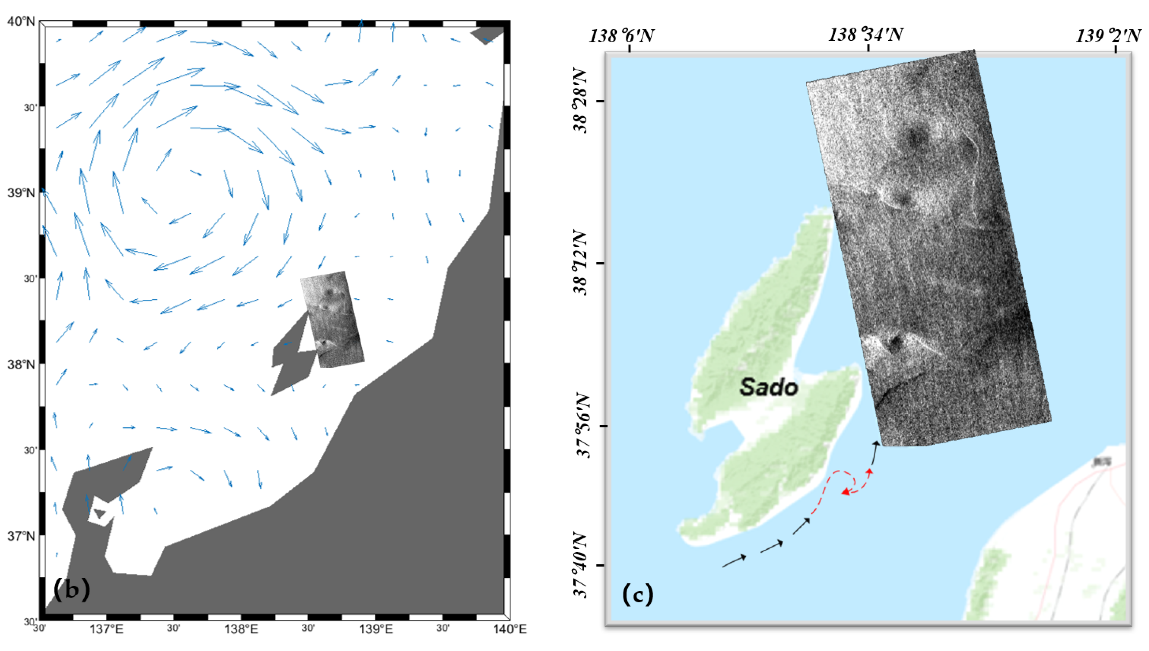
44]. In addition, we performed a long time series analysis using OSCAR data, and the results indicate the presence of ocean eddies in the study area throughout the year. A snapshot of the surface geostrophic velocity field is given in Figure 2b, which shows the presence of a mesoscale eddy with a diameter of about 200 km in the upper left corner and the presence of an eastward surface current found on the southwest side of Sado Island. According to the study on eddy formation mechanisms in the literature [2,43,45], we speculate that the eddies E-1, E-2, and E-3 are formed by the interaction between ocean currents and the northeast and southeast coasts of Sado Island (Figure 2c). In Figure 1a, eddies E-2 and E-3 are relatively faint, and E-1 is more apparent, most probably due to the attenuation of the eddy as it moves from the southwest side of Sado Island to the northeast side. It is worth noting that the observed eddies consist of two parts: bright stripes along the edges and a dark central area. The former is likely due to the interaction of the eddy-induced waves and currents increasing the roughness of the sea surface, resulting in a significant enhancement of the radar backscattering intensity. The latter may be caused by the eddy convergence effect polymerizing the marine oil film, resulting in a weakening of the backscattering intensity. In general, the W-E’s detection is focused on identifying the bright bands (i.e., bright edge areas) resulting from wave–current interaction effects. Therefore, these two components are discussed independently below.
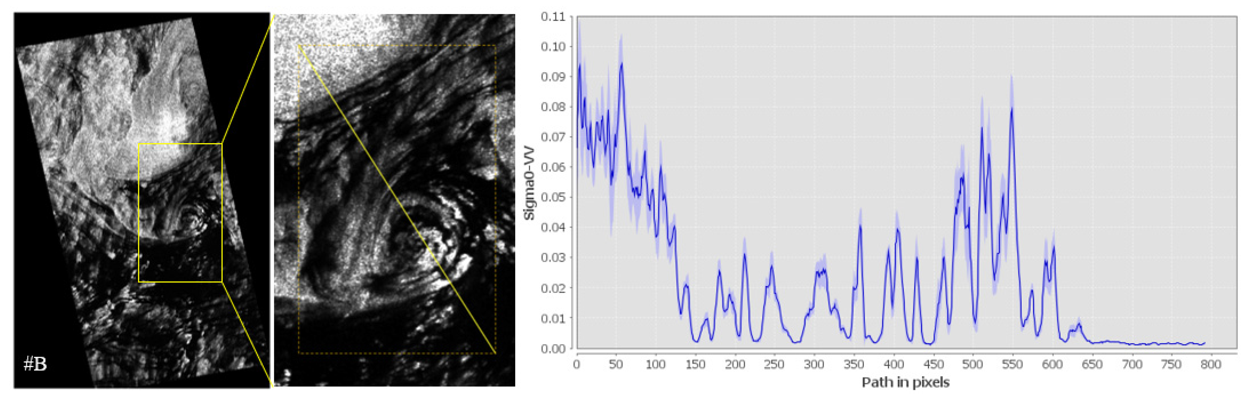
Data #B are located in the Kuroshio region in the northwest Pacific Ocean, which has a complex circulation structure. The westward flowing North Equatorial Current reaches the Philippine coast and bifurcates under the influence of topography, forming the Mindanao Current, which flows toward the equator, and the Kuroshio Current, which flows toward the poles. The Kuroshio Current carries hot and salty equatorial water that gradually intensifies as it flows along the Pacific’s western boundary, and this highly energetic boundary current eventually forms the Kuroshio Extension Zone at 35° N off the coast of Japan. Studies have shown that oceanic eddies are often generated along the Kuroshio tide and its extension. 
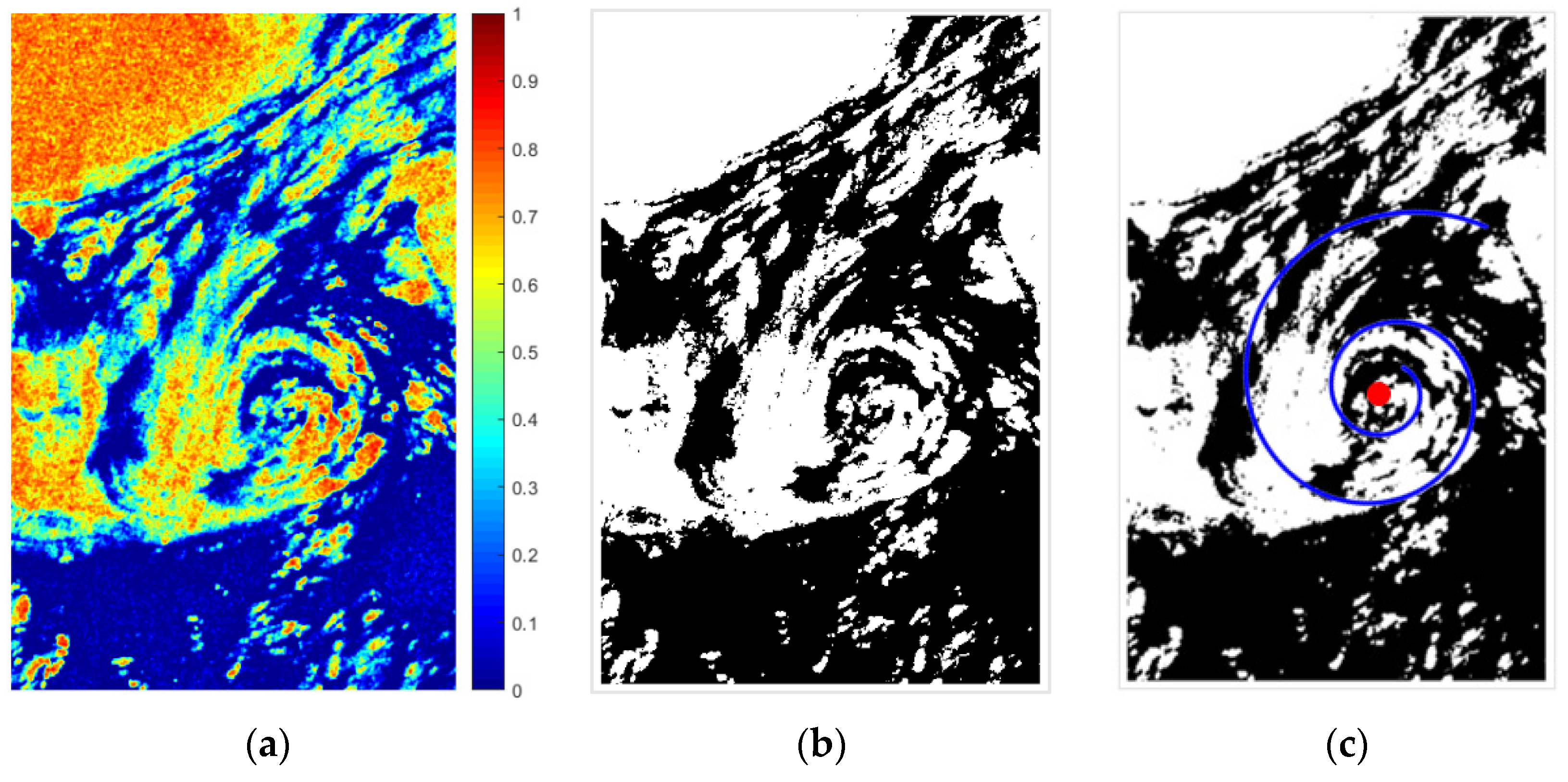
Figure 1b shows the #B VV-polarized backscatter coefficient image. The presence of the oil film produced a significant suppressive effect on short and capillary waves (known as the Marangoni effect) [46]. This weakened the radar echoes and produced a darker appearance in most areas of the image. The oil film-covered region located in the middle of the image contains a region with a distinct spiral morphology, which we determined to be an oceanic eddy for the following reasons: (1) the area covered by the data was the area where the occurrence of eddy currents was frequently observed, and (2) the morphological combination of the region closely matched an eddy as defined in the literature [24]. The eddy diameter is about 11 km. It is supposed that the film acts as a tracer, giving the eddy a specific black spiral line pattern. Detailed data are presented in Table 1.

3. Compact Polarimetric SAR Data Acquisition and Feature Extraction

Compact polarimetric SAR is essentially a DP system. Compared with FP SAR, the system design and maintenance are less complex, and the imaging width is larger. At present, three main modes of CP SAR have been proposed:
  • The π/4 mode of transmitting 45° linearly polarized waves and receiving horizontal (H) and vertical (V) linearly polarized waves [40];
  • The dual circular polarization (DCP) mode that transmits left-hand or right-hand circularly polarized waves and receives left-hand and right-hand circularly polarized waves [47];
  • The hybrid polarization (HP) mode, which transmits left-handed or right-handed circularly polarized waves and receives H and V linearly polarized waves. This mode is also known as the circular transmit and linear receive (CTLR) mode [48].
Compared with the traditional linear DP SAR, the CP SAR can store the phase of the echo signal, and the signal combination method is more flexible. Thus, CP SAR can obtain richer scattering information and achieve similar results to the FP SAR data in numerous applications.

3.1. Compact Polarimetric Data Simulation

Owing to the lack of real CP data, most studies use FP SAR data to reconstruct CP SAR data. Because the CTLR mode has rotational invariance compared with the π/4 mode, the system structure is more straightforward, more stable, and less sensitive to noise than the DCP mode [49]. Therefore, this study predominately focuses on the CTLR mode. The CP scattering vector obtained from the polarized scattering matrix is as follows [50]:
k = E H C E V C = 1 2 S H H S V H S H V S V V 1 ± i = 1 2 S H H ± i S H V S V H ± i S V V
where C indicates the circular polarization and +/− indicates that the system emits a left or right circularly polarized wave (LHC or RHC). This study applied right-hand circular polarization (i.e., CTLR) because circular transmission enabled better reconstruction of pseudo-FP information [49]. From Equation (1), the covariance matrix of the right circularly polarized CP was expressed as
C 2 = k k   * T = C 11 C 12 C 21 C 22 = E R H 2 E R H E R V * E R V E R H * E R V 2
where R indicates the circular polarization, T is a matrix transpose operation, * denotes the complex conjugate, and < > is the spatial average.

3.2. Feature Extraction from Compact Polarimetric SAR Data

Based on the theory of CP data simulations in Section 3.1, the ALOS PALSAR FP SAR data were reconstructed to obtain the CP SAR data. PoLSARpro [51] was used to extract the CP features. The process of extracting CP features in this study is shown in Figure 3. In total, 50 features were used for analysis in this study, and these were predominantly obtained through a combination of polarization components and polarization decomposition. In order to exclude noise from the image, a mean filter was used for image pre-processing prior to performance analysis. These features are summarized in Table 2, which includes 50 CP features and σ images of 4 different polarization channels. Among these features, f1f4 represent σ images of the copolarization and cross-polarization, and c1c4 correspond to the covariance matrix elements of CP SAR. Other features were derived from polarization decomposition methods, with the main ones described below.

3.2.1. Polarimetric Decomposition Based on Stokes Parameters

Aside from the scattering vector and covariance matrix, the Stokes vector (introduced by Raney in 2007 [48]) can also be used to represent the CP. The Stokes vector expressions are as follows:
g = g 0 g 1 g 2 g 3 = E R H 2 + E R V 2 E R H 2 E R V 2 2 R e E R H E R V * 2 I m E R H E R V *
where c5(g0) represents the total power of an electromagnetic wave, c6(g1) represents the horizontal or vertical linear polarization component power, c7(g2) represents the value of the linear polarization component power at 45° or 135°, and c8(g3) is the circularly polarized component power. Re and Im denote the real and imaginary parts, respectively. The Stokes vector can be used to obtain the circular polarization ratio c9(CPR), degree of circular polarization c10(DoCP), degree of linear polarization c11(DoLP), linear polarization ratio c12(LPR), contrast c13(con), orientation angle c14(phi), ellipticity angle c15(tau), and Poincare planisphere parameters (c16–c17: xp, yp). In addition, the polarization degree c18(m), circularity c19(χ), and relative phase c20(δ) can also be obtained using the Stokes vector:
m = g 1 2 + g 2 2 + g 3 2 g 0
s i n 2 χ = g 3 m g 0    χ   45 ° ,   45 °
δ = arctan g 3 g 2    δ   180 ° ,   180 °

3.2.2. m-χ Decomposition

According to the polarization wave dichotomous theory, the covariance matrix of the CP SAR can be divided into depolarized and FP components using the polarization degree (m). Raney et al. [53] concluded that any change in the orientation of the dihedral angle structure may cause a change in the sign of the relative phase (δ) when the emitted electromagnetic wave has a strong line polarization component. Meanwhile, the circularity (χ) is more stable. Thus, a method based on m-χ decomposition was proposed, and its corresponding decomposition is shown in the following equation:
V R V G V B = g 0 m 1 + s i n 2 χ 2 g 0 1 m g 0 m 1 s i n 2 χ 2
where c21(VR), c22(VG), and c23(VB) are the single-bounce (and Bragg) backscattering, double bounce, and randomly polarized constituent, respectively.

3.2.3. H/α Decomposition

Similar to the theory of FP H / α decomposition, Clonde et al. [52] proposed a CP H / α decomposition based on the covariance matrix:
C 2 = 1 λ 1 + λ 2 U 2 p 1 0 0 p 2 U 2 1
This decomposition equation can be used to obtain the eigenvalues λ i i = 1 ,   2 (c24–c25) and probabilities p i i = 1 ,   2 (c26–c27) of the polarization covariance matrix, where λ 1     λ 2 . Using the CP eigenvalues, a series of polarization features based on the eigenvalues can be obtained, such as the CP entropy c28(H), anisotropy c29(A), alpha (c30–c32), lambda (c33), delta (c34–c36), and shannon entropy (c37–c39):
S E = S E I + S E P
S E I = 2 l o g π e T r C 2 2
S E P = l o g 4 d e t C 2 T r C 2 2
In addition, four polarization features can be obtained by combining H and A, which are c40(1mH1mA), c41(1mHA), c42(H1mA), and c43(HA).
Finally, six features were obtained using the three-component compact decomposition and compact RVoG (random volume over ground) decomposition [52], which were the dihedral component power c44(Pd), surface scattering component c45(Ps), volume power c46(Pv), c47(Alpha_s), c48(ms), c49(mv), and c49(phi).

4. Comprehensive Quantification and Evaluation of CP Features for Eddy Detection

4.1. Method and Sample Selection

The Euclidean distance metric was used to measure the contrasts between marine targets, such as ocean eddies, surface slicks, and ocean backgrounds. This metric was also used to compare the contrasts among the 50 selected polarimetric features from CP SAR to quantitatively determine their eddy detection capabilities. The Euclidean distance was defined as follows:
D = m 1 m 2 σ 1 2 + σ 2 2
where m and σ 2 denote the sample mean and variance, respectively, · is the absolute value, and D > 0. A larger Euclidean distance indicatef greater differentiability between the two samples, and vice versa. The above formula indicates that when the mean difference is larger and the variance is smaller, the Euclidean distance is larger between regions, and the separability is larger. Euclidean distance is widely used in many applications, such as sea ice classification, ship target identification [58], and marine oil spill detection [59].
The colored boxes in Figure 4 indicate the selected regions used in the analysis, and regions 50 × 50 pixels in size were used. To ensure sample accuracy and avoid misjudgment, this study selected the most apparent characteristic pixel of the eddy as the input (red boxes in Figure 4, with the white edge line selected for W-E and skeleton line selected for B-E) and the clear and uniform seawater pixel as the ocean background sample (blue boxes in Figure 4). To avoid the influence of local sea state differences and radar signal attenuation, the nearest neighboring clean sea pixels were selected to represent ocean background samples for contrasting with eddies. The subsequent Euclidean distance calculation was conducted based on this principle. Based on the selection of samples from the two regions (eddies and sea surface), the mean and variance of the samples from each region in each polarimetric feature image were counted, and the Euclidean distance between the eddies and each region was calculated according to Equation (12), which was also used to measure the detection performance of the CP feature parameters for the ocean eddies and the differentiation ability of different regions.

4.2. Evaluation of Different Features by Euclidean Distance

4.2.1. White Eddy

Figure 5 shows the Euclidean distances (D) between the eddy edge (Ee), center (Ec), and ocean background (S) for the 3 eddies in the 50 CP feature images extracted using data #A. The colored solid lines are DEe-S (Euclidean distance between Ee and S), and the colored dashed lines represent DEc-S (Euclidean distance between Ec and S). It can be seen that the trends of DEe-S and DEc-S were relatively consistent across the features, and DE1e-S (Euclidean distance of the E-1 edge) was the largest overall, which was both easily visible and distinguishable. In general, the detection of W-E focused on the identification of bright bands resulting from wave–current interaction effects. Among the four radar backscatter coefficients (f1( σ H H ), f2( σ H V ), f3( σ V H ), and f4( σ V V )), the DE-S (Euclidean distance between Ee, Ec, and the marine background) value in the f1( σ H H ) image was the largest, and the CP features c44(Pd), c38(SEI), c21(Dbl), c5(g0), c8(g3), c24(l1), c33(lambda), c48(ms), c37(SE), and c45(Ps) had better eddy detection performance and were improved over the original radar image f1( σ H H ). Figure 6 presents all CP feature images with better W-E detection performance. It can be seen that E-1 is clearly visible in all the feature images both at Ee and Ec. Conversely, E-2 and E-3 are relatively blurred, and the Ee values are submerged in the ocean background, most likely because of the relatively weak vortex intensity from E-2 and E-3.
The Euclidean distance between the eddy and ocean background under each CP feature was comprehensively analyzed. The 50 CP features were divided into 3 levels according to their W-E detection performance. Moreover, the visualization performance of the 50 CP features was evaluated for eddies E-1, E-2, and E-3. The results are presented in Table 3. In Level 1, DE-S > 1, and the eddy characteristics in the image were apparent. Thus, the eddy could be effectively distinguished from the ocean background and directly applied for future ocean eddy detection and recognition studies. In Level 2, the DE-S value ranged from 1 to 0.9, and the eddy feature was relatively weak but could be distinguished by the naked eye. In Level 3, the DE-S value was between 0.9 and 0.8. All eddies were relatively fuzzy, and only E-1, with a larger vortex intensity, could be distinguished from the ocean background. Meanwhile, E-2 and E-3, with weaker vortex intensities, were submerged within the ocean background. The remaining features are not included in the table because of the low contrast between the eddies and the ocean background in the images, hindering the effective differentiation of the eddies.

4.2.2. Black Eddy

Figure 7 shows the Euclidean distances between the eddy helix (Eb), the coupling region (EW) of the seawater and Eb, the oil film (O), and seawater (S) for the CP feature for data #B. The figure shows that DEb-S (Euclidean distance between Eb and S) and DO-S (Euclidean distance between O and S) followed the same trend in most of the feature images, with DEb-S being slightly larger but less different. The DEb-S value of f4( σ V V ) was the largest among the four polarization channels, which was different from f1( σ H H ) for the W-E, indicating that the backscatter coefficient images of the different polarization channels differed in their ability to characterize B-E and W-E. The HH polarimetric proved to be the most effective for characterizing B-E, and the VV polarimetric was most effective for characterizing the W-E. In addition, the CP features of the c41(1mHA), c28(H), c39(SEP), c38(SEI), c37(SE), c27(p2), c18(m), c29(A), c26(p1), c21(Dbl), c42(H1mA), and c9(CPR) images had larger DEb-S values (i.e., better detection performances) and outperformed the original radar backscatter coefficient image f4( σ V V ). Overall, DEw-S (Euclidean distance between EW and S) was small, with a mean distance of 0.355. The cross-sectional distribution of the eddy region in the f4( σ V V ) image (Figure 8) shows that the eddy helix was similar in intensity than the oil film scattering, and the area around Eb was slightly smaller than that of S scattering; however, this difference was small.
The above phenomenon can be explained by the B-E SAR imaging mechanism, where the formation is caused by the suppression of surface waves by surfactant materials accumulated in regions of current shear and convergence, and the area around the black spiral line is actually a clean sea. Thus, DEb-S and DO-S were approximately equal, while the DEw-S value was smaller. The above better-performing CP feature images and f4( σ V V ) images are shown in Figure 9, where the eddy contours can be clearly distinguished.
Similarly, the Euclidean distance between B-E and the ocean background was analyzed for each CP feature. The 50 CP features were divided into three levels according to their ability to detect eddies. Moreover, the visualization of Eb and O was assessed for each level. The results are shown in Table 4, with DE-S > 6 for Level 1, DE-S values between 4 and 5 for Level 2, and DE-S values between 1 and 4 for Level 3. Features with D < 1 were not included in the table.

5. Detection Results

In the previous section, 10 (13) CP polarization features with better W-E (B-E) identification performance were identified using the Euclidean distance. In this section, the results of the eddy extraction experiments are presented, which were conducted using these features to verify the superiority of these features in eddy detection.

5.1. White Eddy

As shown in Section 4.2.1, the 10 polarization features (c44(Pd), c38(SEI), c21(Dbl), c5(g0), c8(g3), c24(l1), c33(lambda), c48(ms), c37(SE), and c45(Ps)) had better W-E characterization ability. In this section, the above features are used for W-E extraction, and it should be noted that since the detection of W-E is mainly to identify bright bands generated by wave–current interaction, only the edges of W-E are discussed in this section. The eddy detection results are shown with polarization feature c42(Pd) as an example. Figure 10 gives the comparison of the detection results for all three eddies (E-1, E-2, and E-3) in the CP feature c42(Pd) image. Figure 10a–c shows the eddy slices in the feature images, and it can be seen that the eddy visibility decreased sequentially. Figure 10d–f shows the eddy detection results based on the k-means classification algorithm (k = 2) [60], with the ocean background in white and the extracted W-E edges in black. The detection results show that the edges were more seriously confused with the seawater. Among them, the detection result of E-1 was relatively good, and most of the eddy edges could be separated from the ocean background. This may have been caused by the eddy intensity as well as the local sea state. Figure 10g–i shows the three-dimensional image of the eddy region in the feature image, and it is noteworthy that the eddy centers had an obvious height difference from the eddy edges. The intensity of E-1 was relatively large, and the roughness of the sea surface caused by wave–current interaction was greater, which resulted in a larger difference in the backscattering between the eddy edge and the ocean background, therefore having a relatively good detection result. In addition, in order to describe the eddy detection accuracy quantitatively, we used the subjective identification of eddies by trained experts as the expert interpretation results and compared the detection results of the eddies in the above 10 features with the expert interpretation results to obtain the eddy detection accuracy (Table 5). It can be seen that the average detection accuracies of the 10 features were 69.83% (E-1), 34.72% (E-2), and 32.71% (E-3), all of which were better than the traditional σ H H (66.67%, 27.01%, and 26.12%, respectively).

5.2. Black Eddy

Similarly, this section presents the results of 13 CP features with better B-E characterization ability, such as c41(1mHA), c28(H), c39(SEP), c38(SEI), c37(SE), c27(p2), c18(m), c29(A), c26(p1), c21(Dbl), c42(H1mA), and c9(CPR), that were used for B-E extraction. The eddy detection results are shown with the optimal CP feature c41(1mHA). The eddy detection result in the CP feature c41(1mHA) image is given in Figure 11, where Figure 11a is the eddy region slice in the feature image, and it can be seen that the eddy had a distinct spiral structure. Figure 11b shows the eddy detection results based on the k-means classification algorithm (k = 2), where white is the ocean background and black is the eddy extraction results, and the results show that the eddies could be effectively separated from the ocean background. In order to quantitatively describe the eddy detection performance, we analyzed the detection results of the eddies in the above 13 CP features by expert decoding to obtain the eddy detection accuracy (Table 6). It can be seen that the detection accuracy in all 13 CP features was better than that of the traditional σ V V (78.47%) and that the improved accuracy reached up to 95.64% (1mHA).
In addition, to explore the potential of SAR in detecting the eddy refinement structure, we conducted a study on eddy spiral structure fitting and eddy center location extraction. Yang et al. [26] showed that the morphology of the eddies was closer to the logarithmic helix, so the logarithmic helix was selected to fit the B-E in this study. The polar equation of the logarithmic helix is as follows:
r = a e θ c o t α = a e b θ ;   b = c o t α
where r is the polar diameter, θ is the polar angle, a is the value of r when θ = 0 o , α is the angle between the polar diameter and the tangent line, and b affects the degree of bending of the helix. In this study, the optimal logarithmic helix parameters a and b were obtained by fitting manually selected eddy profile feature points to determine the eddy center location. The results are shown in Figure 11c, where the blue helix is the optimal logarithmic helix obtained by fitting and the red dot is the obtained eddy center location.

6. Discussion

The data used in this article were the two FP ALOS PALSAR images (#A and #B) collected from the sea around Japan. These two scenes are covered with suspected W-E and B-E, respectively. In terms of eddy existence authenticity verification, Section 2 discussed the flow field characteristics of the study area, the frequency of ocean eddy occurrence, the eddy formation mechanism, and the resultant eddy shape and then compared the findings with the eddy research data from the other literature [24]. The results show that the eddy defined in this paper was reliable.
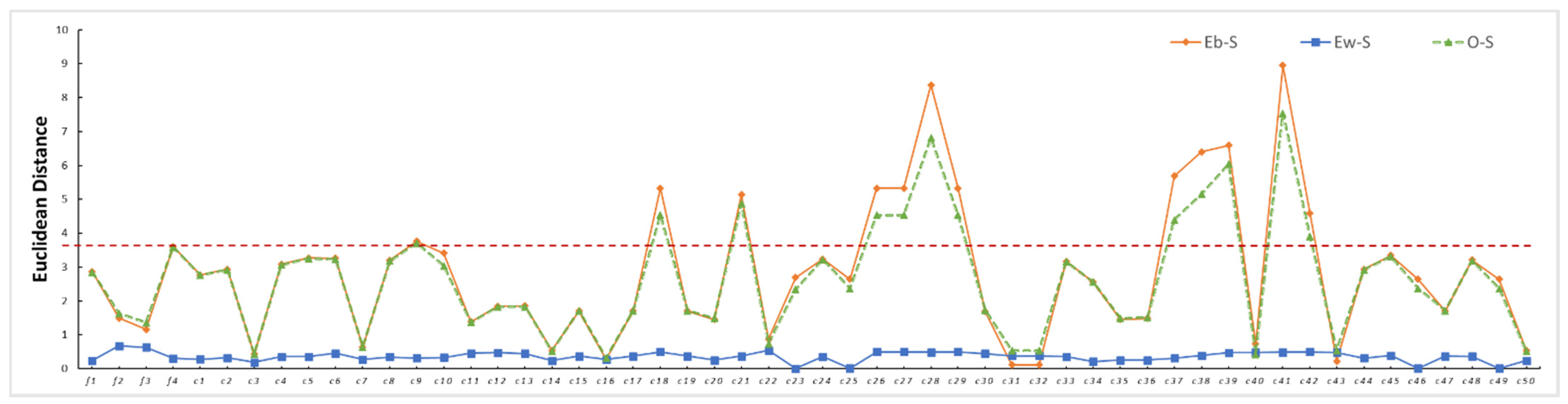
In 
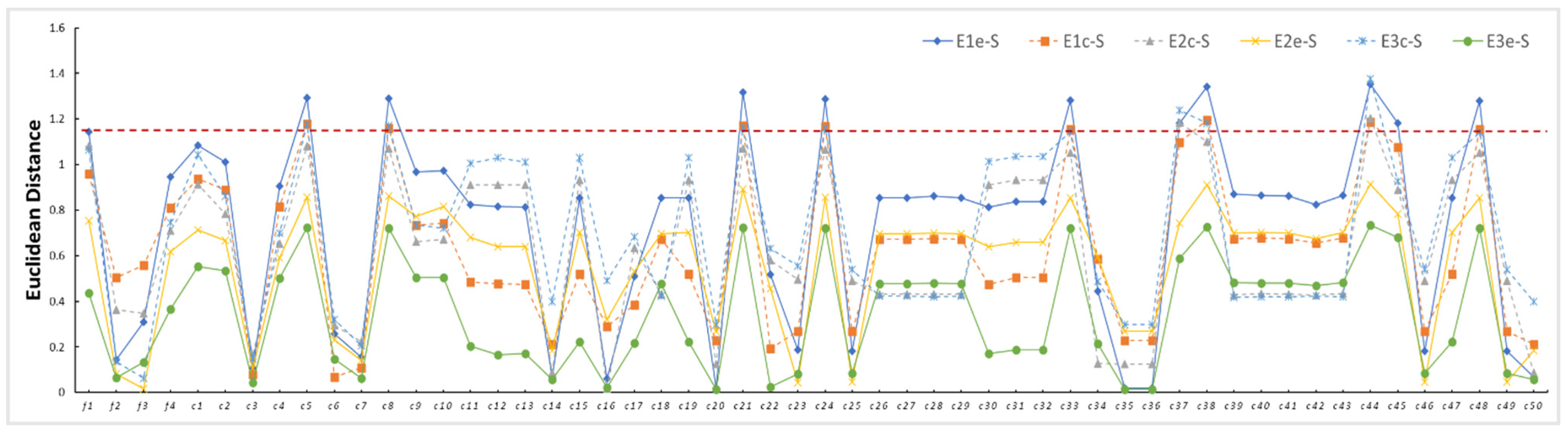
Section 4.2, the Euclidean distance was used to analyze the eddy detection performance of 50 CP features. By comparing Figure 5 and Figure 7 of that section, we found that the best Euclidean distance between W-E and the ocean background was only 1.35, which was much smaller than the Euclidean distance between B-E and the ocean background (average value: 2.84). This was possibly the result of the different imaging mechanisms of the two eddies in SAR as follows. The B-E is caused by the tracing of film [61], and the natural film generally appears in the SAR image at low to moderate wind speeds (3–5 m/s) [62]. At higher wind speeds, the surfactant film starts to disrupt, and as a result, the dark spiral lines representing B-E disappear. Thus, the eddies appear in the SAR image only as a result of the wave–current interaction along the current shear lines, which manifests as a bright area [24]. However, it should also be considered that high sea conditions will reduce the contrast between W-E and the ocean background, thus manifesting itself as a low Euclidean distance. It is worth mentioning that due to the harsh imaging mechanism of W-E, the amount of W-E SAR data that could be found was very small. Therefore, most research on eddy detection by SAR application is focused on B-E. In addition, a similar finding resulted from the eddy detection results presented in Section 5, namely the detection accuracy of W-E being lower than that of B-E. The phenomenon was that the detection accuracy of W-E was lower than that of B-E. Therefore, this difference in Euclidean distance and detection accuracy was consistent with the actual situation of the two eddies with different imaging mechanisms.
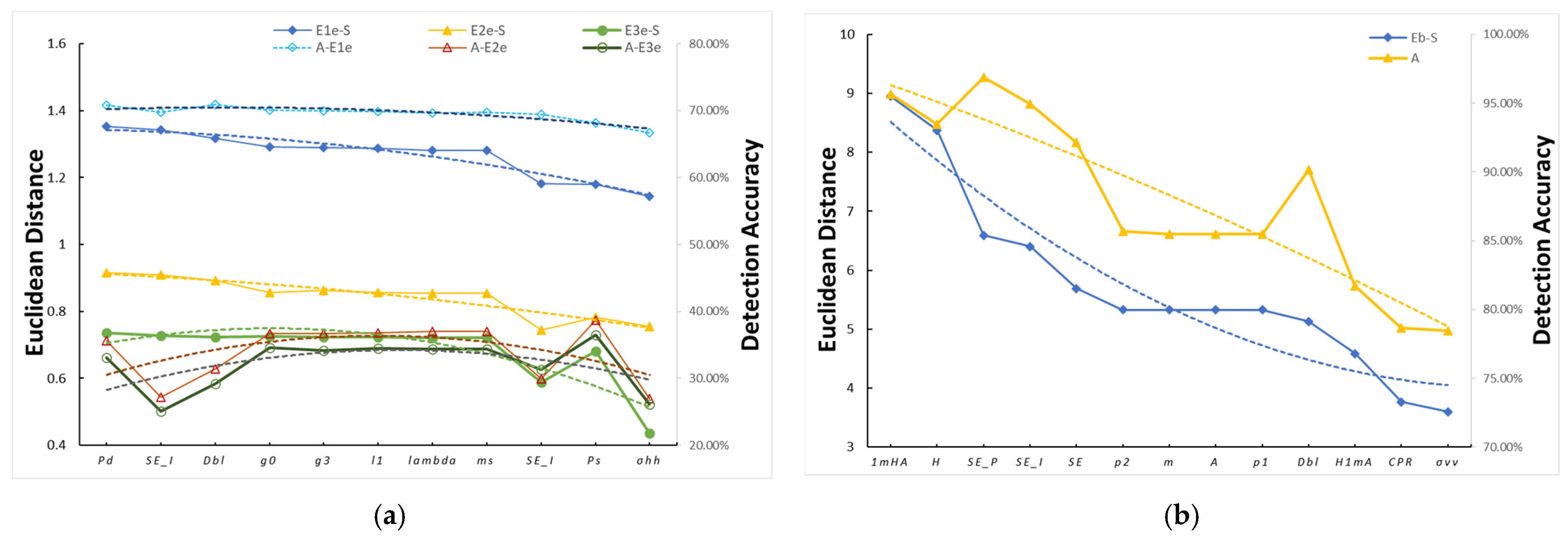
When comparing the Euclidean distance calculation results and the eddy detection accuracy, we found that they were consistent. Figure 12 gives the variation of the CP feature Euclidean distance and eddy detection accuracy, where the colored dashed lines in the figure are the results of the third-order polynomial fit. The figure shows that for E-1 and B-E, the eddy detection accuracy decreased with the decrease in the Euclidean distance, which proves the reliability of using the Euclidean distance to analyze the eddy detection performance of the CP features. However, E-2 and E-3 were severely confused with the ocean background, and their accuracy was low and contingent. This means that the detection accuracy did not produce the same trend as the Euclidean distance; however, this does not affect the above conclusions.
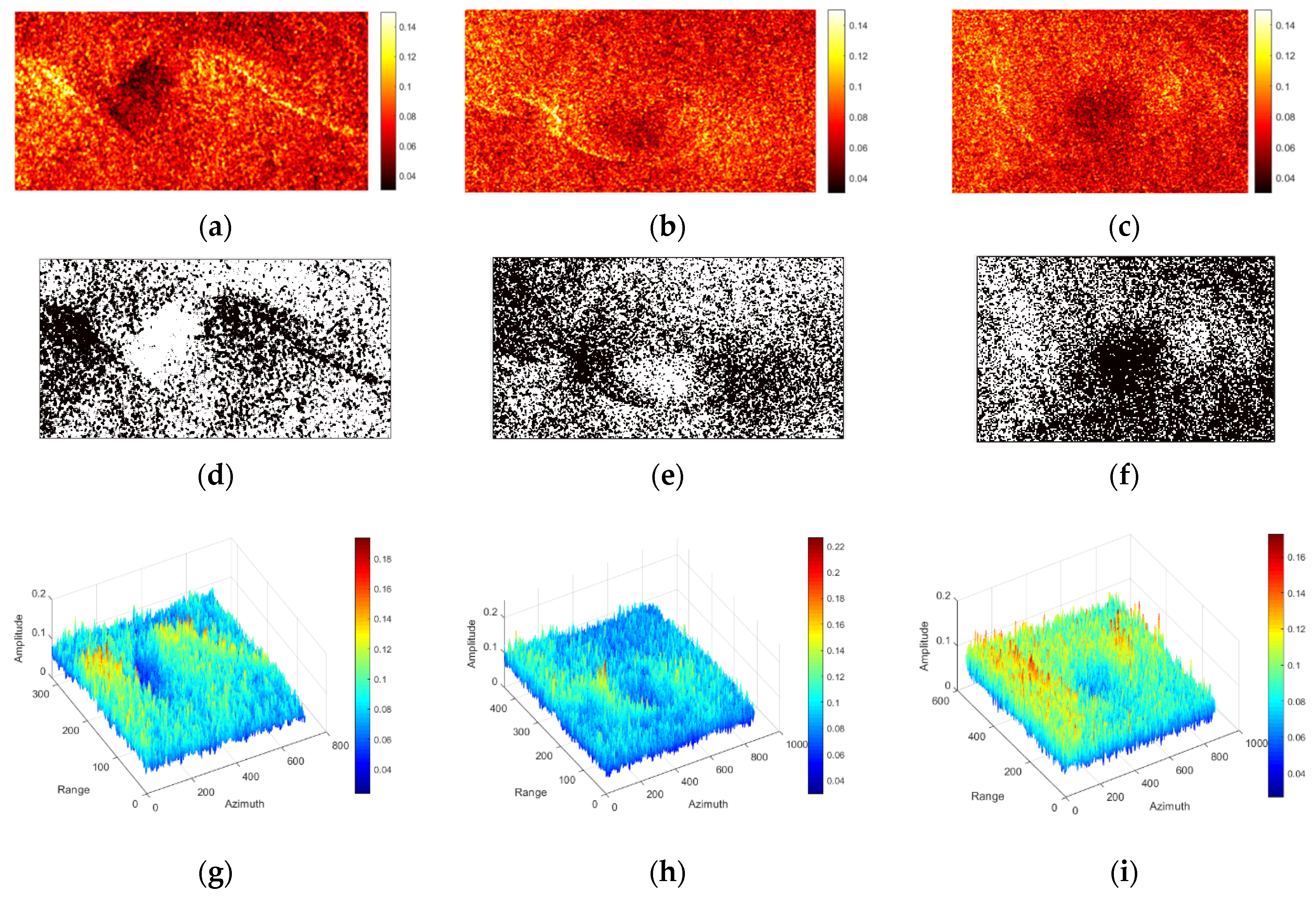
In Section 5.2, the location of the eddy center was determined in the B-E detection result (Figure 11c) using the method based on logarithmic spiral edge fitting for eddy information extraction in the SAR image. The eddy shape described by this method agreed with the actual one, and furthermore, the results of the eddy center’s position agreed with the reference information provided manually. This demonstrates the great application potential of CP SAR in eddy information extraction and eddy refinement structure research.
Compared with satellite altimeters for mesoscale eddy detection, SAR images are more often used to observe sub-mesoscale and small mesoscale eddies (diameter < 10 km). Such ocean eddies are smaller in scale, shorter in duration, and faster in variability, while their edges are more filamentary and irregular, and their formation mechanisms are different from those of mesoscale eddies [4]. Considering this, compared with satellite altimeters and optical sensors, SAR is not affected by light and has a higher resolution, which makes SAR more relevant for such ocean eddy detection. In future research, we will carry out work on the inversion of the eddy parameters (e.g., eddy center position, diameter, and edge size) using a variety models. Meanwhile, considering the current challenges, such as the surge of SAR data volume, we will combine cutting-edge technologies such as deep learning to develop better SAR eddy detection algorithms.

7. Conclusions

As an emerging direction of polarimetric SAR, the CP SAR adopts a unique DP SAR system, which enables large-amplitude broad observations of up to 350 km and fully preserves the polarization scattering information, giving it significant potential application in the large-scale detection of ocean phenomena and targets. However, relatively few studies have been conducted on eddy detection using CP SAR data. Before this study, the response of CP SAR to ocean eddies was unknown, which severely restricted the application of CP SAR for ocean eddy monitoring. Therefore, in this study, ALOS PALSAR FP SAR data containing W-E and B-E were used to simulate the CP SAR data to evaluate the application potential of CP SAR for ocean eddy identification and dynamic monitoring. Based on this, the performance of the CP features in detecting ocean eddies was further discussed. The results showed that among the 50 CP features, Pd, SEI, Dbl, g0, g3, l1, lambda, ms, SE, and Ps had better detection performance for W-E. Moreover, it was found that m, A, p1, Dbl, H1mA, and CPR could more accurately determine B-E.

Author Contributions

Conceptualization, S.S.; data curation, Y.H.; formal analysis, S.S.; investigation, H.H. and W.J.; methodology, J.Y. and H.H.; project administration, J.Y.; resources, J.Y.; software, S.S.; supervision, Y.L.; validation, C.Y., W.J. and Y.H.; visualization, C.Y., W.J. and Y.H.; writing—original draft preparation, S.S.; writing—review and editing, S.S. and J.Y. All authors have read and agreed to the published version of the manuscript.

Funding

This research was funded by the National Natural Science Foundation of China, grant numbers 41976189 and 41976190; the Key Special Project for Introduced Talents Team of Southern Marine Science and Engineering Guangdong Laboratory (Guangzhou), grant number GML2019ZD0301; the Guangdong Innovative and Entrepreneurial Research Team Program, grant number 2016ZT06D336; and GDAS’ Project of Science and Technology Development, grant number 2019GDASYL-0301001; Guangxi Science and Technology Key R&D Program Project, grant number AB20297037.

Data Availability Statement

Not applicable.

Conflicts of Interest

The authors declare no conflict of interest.

References

  1. Karimova, S. Spiral eddies in the Baltic, Black and Caspian seas as seen by satellite radar data. Adv. Space Res. 2012, 50, 1107–1124. [Google Scholar] [CrossRef]
  2. Ivanov, A.Y.; Ginzburg, A.I. Oceanic eddies in synthetic aperture radar images. J. Earth Syst. Sci. 2002, 111, 3. [Google Scholar] [CrossRef] [Green Version]
  3. Robinson, A.R. Overview and Summary of Eddy Science. In Eddies in Marine Science; Springer: Berlin, Germany, 1983; pp. 3–15. [Google Scholar]
  4. Chen, G.; Yang, J.; Tian, F.L.; Chen, S.G.; Zhao, C.F.; Tang, J.W.; Liu, Y.J.; Wang, Y.N.; Yuan, Z.H.; He, Q.; et al. Remote sensing of oceanic eddies: Progresses and challenges. Natl. Remote Sens. Bull. 2021, 25, 302–322. [Google Scholar] [CrossRef]
  5. Pérez-Muñuzuri, V.; Huhn, F. The role of mesoscale eddies time and length scales on phytoplankton production. Nonlinear Process. Geophys. 2010, 17, 177–186. [Google Scholar] [CrossRef] [Green Version]
  6. Williams, S.; Hecht, M.; Petersen, M.; Strelitz, R.; Maltrud, M.; Ahrens, J.; Hlawitschka, M.; Hamann, B. Visualization and Analysis of Eddies in a Global Ocean Simulation. Comput. Graph. Forum 2011, 30, 991–1000. [Google Scholar] [CrossRef]
  7. Alpers, W.; Brandt, P.; Lazar, A.; Dagorne, D.; Sow, B.; Faye, S.; Hansen, M.W.; Rubino, A.; Poulain, P.-M.; Brehmer, P. A small-scale oceanic eddy off the coast of West Africa studied by multi-sensor satellite and surface drifter data. Remote Sens. Environ. 2013, 129, 132–143. [Google Scholar] [CrossRef]
  8. Dong, C.; Nencioli, F.; Liu, Y.; McWilliams, J.C. An automated approach to detect oceanic eddies from satellite remotely sensed sea surface temperature data. IEEE Geosci. Remote Sens. Lett. 2011, 8, 1055–1059. [Google Scholar] [CrossRef]
  9. Zhang, C.; Li, H.; Liu, S.; Shao, L.; Zhao, Z.; Liu, H. Automatic detection of oceanic eddies in reanalyzed SST images and its application in the East China Sea. Sci. China Earth Sci. 2015, 58, 2249–2259. [Google Scholar] [CrossRef]
  10. Marcello, J.; Eugenio, F.; Estrada-Allis, S.; Sangra, P. Segmentation and tracking of anticyclonic eddies during a submarine volcanic eruption using ocean colour imagery. Senses 2015, 15, 8732–8748. [Google Scholar] [CrossRef] [Green Version]
  11. He, Z.; Wang, D.; Chen, J.; Hu, J. Eddy structure in south China sea from satellite tracked surface drifting buoys and satellite remote sensing sea surface height. J. Trop. Oceanogr. 2001, 20, 27–35. [Google Scholar]
  12. Lyzenga, D.; Wackerman, C. Detection and classification of ocean eddies using ERS-1 and aircraft SAR images. Variations 1997, 414, 1267. [Google Scholar]
  13. Topouzelis, K.; Kitsiou, D. Detection and classification of mesoscale atmospheric phenomena above sea in SAR imagery. Remote Sens. Environ. 2015, 160, 263–272. [Google Scholar] [CrossRef]
  14. Magalhães, J.; Alpers, W.; Santos-Ferreira, A.; da Silva, J. Surface Wave Breaking Caused by Internal Solitary Waves: Effects on Radar Backscattering Measured by SAR and Radar Altimeter. Oceanography 2021, 34, 166–176. [Google Scholar] [CrossRef]
  15. De Macedo, C.R.; da Silva, J.C.B. Internal Wave Dark-Band Signatures in ALOS-PALSAR Imagery Revealed by the Standard Deviation of the Co-Polarized Phase Difference. Remote Sens. 2020, 12, 2372. [Google Scholar] [CrossRef]
  16. Isoguchi, O.; Ebuchi, N.; Shimada, M. Meso- and Submeso-Scale Ocean Front Detection Using SAR and Optical Data. In Proceedings of the IEEE International Geoscience and Remote Sensing Symposium, Beijing, China, 10–15 July 2016. [Google Scholar]
  17. Fu, L.L.; Ferrari, R. Observing oceanic submesoscale processes from space. Eos Trans. Am. Geophys. Union 2008, 89, 488. [Google Scholar] [CrossRef]
  18. Karimova, S.; Gade, M. Submesoscale Eddies Seen by Spaceborne Radar. In Proceedings of the EMEC 10-MEDCOAST, Marmaris, Turkey, 30 October–3 November 2013; pp. 665–676. [Google Scholar]
  19. Di Giacomo, P.M.; Holt, B. Satellite observations of small coastal ocean eddies in the Southern California Bight. J. Geophys. Res. Ocean. 2001, 106, 22521–22543. [Google Scholar] [CrossRef]
  20. Xu, G.; Yang, J.; Dong, C.; Chen, D.; Wang, J. Statistical study of submesoscale eddies identified from synthetic aperture radar images in the Luzon Strait and adjacent seas. Int. J. Remote Sens. 2015, 36, 4621–4631. [Google Scholar] [CrossRef]
  21. Alpers, W.; Hühnerfuss, H. The damping of ocean waves by surface films: A new look at an old problem. J. Geophys. Res. Ocean. 1989, 94, 6251–6265. [Google Scholar] [CrossRef]
  22. Johannessen, J.A.; Shuchman, R.A.; Johannessen, O.M.; Davidson, K.L.; Lyzenga, D.R. Synthetic aperture radar imaging of upper ocean circulation features and wind fronts. J. Geophys. Res. Ocean. 1991, 96, 10,411–10,422. [Google Scholar] [CrossRef] [Green Version]
  23. Johannessen, J.; Digranes, G.; Espedal, H.; Johannessen, O.; Samuel, P.; Browne, D.; Vachon, P. SAR ocean feature catalogue. ESA Spec. Publ. 1994, 1174, 106. [Google Scholar]
  24. Karimova, S.S.; Gade, M. Eddies in the Red Sea as Seen by Satellite SAR Imagery. In Remote Sensing of the African Seas; Gade, V.B.a.M., Ed.; Springer: Berlin/Heidelberg, Germany, 2014; pp. 357–378. [Google Scholar]
  25. Was, N.; Andharia, H. Determination of the velocity of ocean gyres through Synthetic Aperture Radar. Int. J. Remote Sens. 1987, 8, 243–249. [Google Scholar] [CrossRef]
  26. Min, Y.; Jin-Song, C. A Method Based on Logarithmic Spiral Edge Fitting for Information Extraction of Eddy in the SAR Image. J. Radars 2013, 2, 243–249. [Google Scholar] [CrossRef]
  27. Schuler, D.L.; Lee, J.S. Mapping ocean surface features using biogenic slick-fields and SAR polarimetric decomposition techniques. IEE Proc. Radar Sonar Navig. 2006, 153, 260–270. [Google Scholar] [CrossRef]
  28. Huang, D.; Du, Y.; He, Q.; Song, W.; Liotta, A. DeepEddy: A simple deep architecture for mesoscale oceanic eddy detection in SAR images. In Proceedings of the IEEE 14th International Conference on Networking, Sensing and Control (ICNSC), Calabria, Italy, 16–18 May 2017; pp. 673–678. [Google Scholar]
  29. Friedman, K.S.; Li, X.; William, G.P. Eddy Detection Using RADARSAT-1 Synthetic Aperture Radar. In Proceedings of the International Geoscience and Remote Sensing Symposium, Anchorage, Alaska, 20–24 September 2004. [Google Scholar]
  30. Liu, A.K.; Peng, C.Y.; Chang, S.-S. Wavelet analysis of satellite images for coastal watch. IEEE J. Ocean. Eng. 1997, 22, 9–17. [Google Scholar] [CrossRef]
  31. Liu, A.; Hsu, M.-K. Deriving Ocean Surface Drift Using Multiple SAR Sensors. Remote Sens. 2009, 1, 266–277. [Google Scholar] [CrossRef] [Green Version]
  32. Lorenzzetti, J.A.; Kampel, M.; Bentz, C.; Torres, A., Jr. A Meso-Scale Brazil Current Frontal Eddy: Observations by ASAR, RADARSAT-1 Complemented with Visible and Infrared Sensors, in situ Data and Numerical Modeling. In Advances in SAR Oceanography from Envisat and ERS Misions, Proceedings of SEASAR, Frascati, Italy, 23–26 January 2006; Citeseer: Princeton, NJ, USA, 2006; pp. 23–26. [Google Scholar]
  33. Yamaguchi, S.; Kawamura, H. SAR-imaged spiral eddies in Mutsu Bay and their dynamic and kinematic models. J. Oceanogr. 2009, 65, 525–539. [Google Scholar] [CrossRef]
  34. Wang, Y.; Yang, M.; Chong, J. SAR image simulation method for oceanic eddies. J. Radars 2019, 8, 382–390. [Google Scholar] [CrossRef]
  35. Buono, A.; Nunziata, F.; Migliaccio, M. Analysis of Full and Compact Polarimetric SAR Features Over the Sea Surface. IEEE Geosci. Remote Sens. Lett. 2016, 13, 1527–1531. [Google Scholar] [CrossRef]
  36. Li, Y.; Zhang, Y.; Chen, J.; Zhang, H. Improved Compact Polarimetric SAR Quad-Pol Reconstruction Algorithm for Oil Spill Detection. IEEE Geosci. Remote Sens. Lett. 2014, 11, 1139–1142. [Google Scholar] [CrossRef]
  37. Buono, A.; de Macedo, C.R.; Nunziata, F.; Velotto, D.; Migliaccio, M. Analysis on the Effects of SAR Imaging Parameters and Environmental Conditions on the Standard Deviation of the Co-Polarized Phase Difference Measured over Sea Surface. Remote Sens. 2018, 11, 18. [Google Scholar] [CrossRef] [Green Version]
  38. Yin, J.; Yang, J.; Zhou, L.; Xu, L. Oil Spill Discrimination by Using General Compact Polarimetric SAR Features. Remote Sens. 2020, 12, 479. [Google Scholar] [CrossRef] [Green Version]
  39. Souyris, J.C.; Mingot, S. Polarimetry based on one transmitting and two receiving polarizations: The π/4 mode. In Proceedings of the IEEE International Geoscience and Remote Sensing Symposium, Toronto, ON, Canada, 24–28 June 2002. [Google Scholar]
  40. Souyris, J.C.; Imbo, P.; Fjortoft, R.; Sandra, M.; Jong-Sen, L. Compact polarimetry based on symmetry properties of geophysical media: The/spl pi//4 mode. IEEE Trans. Geosci. Remote Sens. 2005, 43, 634–646. [Google Scholar] [CrossRef]
  41. Dabboor, M.; Geldsetzer, T. On the classification of sea ice types using simulated radarsat constellation mission (RCM) compact polarimetric SAR parameters. In Proceedings of the ASPRS 2014 Annual Conference, Louisville, KY, USA, 23–28 March 2014; pp. 23–28. [Google Scholar]
  42. Misra, T.; Rana, S.; Bora, V.; Desai, N.; Rao, C.; Jyothi, R. SAR Payload of Radar Imaging Satellite (RISAT) of ISRO. In Proceedings of the 6th European Conference on SAR, EUSAR-06, Dresden, Germany, 16–18 May 2006; pp. 16–18. [Google Scholar]
  43. Nencioli, F.; Dong, C.; Dickey, T.; Washburn, L.; McWilliams, J.C. A Vector Geometry–Based Eddy Detection Algorithm and Its Application to a High-Resolution Numerical Model Product and High-Frequency Radar Surface Velocities in the Southern California Bight. J. Atmos. Ocean. Technol. 2010, 27, 564–579. [Google Scholar] [CrossRef]
  44. Johannessen, J.A.; Shuchman, R.A.; Digranes, G.; Lyzenga, D.R.; Wackerman, C.; Johannessen, O.M.; Vachon, P.W. Coastal ocean fronts and eddies imaged with ERS 1 synthetic aperture radar. J. Geophys. Res. Ocean. 1996, 101, 6651–6667. [Google Scholar] [CrossRef] [Green Version]
  45. Le Vu, B.; Stegner, A.; Arsouze, T. Angular Momentum Eddy Detection and Tracking Algorithm (AMEDA) and Its Application to Coastal Eddy Formation. J. Atmos. Ocean. Technol. 2018, 35, 739–762. [Google Scholar] [CrossRef]
  46. Fingas Merv, B.C. A Review of Oil Spill Remote Sensing. Sensors 2017, 18, 91. [Google Scholar] [CrossRef] [Green Version]
  47. Stacy, N.; Preiss, M. Compact polarimetric analysis of X-band SAR data. In Proceedings of the European Conference on Syntethic Aperture Radar EUSAR, Dresden, Germany, 16–18 May 2006. [Google Scholar]
  48. Raney, R.K. Hybrid-polarity SAR architecture. IEEE Trans. Geosci. Remote Sens. 2007, 45, 3397–3404. [Google Scholar] [CrossRef] [Green Version]
  49. Nord, M.E.; Ainsworth, T.L.; Jong-Sen, L.; Stacy, N.J.S. Comparison of Compact Polarimetric Synthetic Aperture Radar Modes. IEEE Trans. Geosci. Remote Sens. 2009, 47, 174–188. [Google Scholar] [CrossRef]
  50. Li, H.; Perrie, W.; He, Y.; Lehner, S.; Brusch, S. Target Detection on the Ocean With the Relative Phase of Compact Polarimetry SAR. IEEE Trans. Geosci. Remote Sens. 2013, 51, 3299–3305. [Google Scholar] [CrossRef]
  51. Haijiang, W. Study on Classification Methods of Polarimetric SAR Images. Ph.D. Thesis, University of Electronic Science and Technology of China, Chengdu, China, 2008. [Google Scholar]
  52. Cloude, S.; Goodenough, D.; Chen, H. Compact Decomposition Theory. IEEE Geosci. Remote Sens. Lett. 2012, 9, 28–32. [Google Scholar] [CrossRef]
  53. Raney, R.K.; Cahill, J.; Patterson, G.W.; Bussey, D. The m-chi decomposition of hybrid dual-polarimetric radar data with application to lunar craters. J. Geophys. Res. Planets 2012, 117, 5093–5096. [Google Scholar] [CrossRef]
  54. Ainsworth, T.L.; Cloude, S.R.; Lee, J.S. Eigenvector Analysis of Polarimetric SAR Data. In Proceedings of the IEEE International Geoscience & Remote Sensing Symposium, Toronto, ON, Canada, 24–28 May 2002. [Google Scholar]
  55. Lee, J.S.; Pottier, E. Polarimetric Radar Imaging: From Basics to Applications; CRC Press: Boca, Raton, FL, USA, 2009. [Google Scholar]
  56. Refregier, P.; Morio, J. Shannon entropy of partially polarized and partially coherent light with Gaussian fluctuations. J. Opt. Soc. Am. A Opt. Image Sci. Vis. 2006, 23, 3036–3044. [Google Scholar] [CrossRef] [PubMed]
  57. Cloude, S.R.; Pottier, E. An entropy based classification scheme for land applications of polarimetric SAR. IEEE Trans. Geosci. Remote Sens. 1997, 35, 68–78. [Google Scholar] [CrossRef]
  58. Cao, C.; Zhang, J.; Meng, J.; Zhang, X.; Mao, X. Analysis of Ship Detection Performance with Full-, Compact- and Dual-Polarimetric SAR. Remote Sens. 2019, 11, 2160. [Google Scholar] [CrossRef] [Green Version]
  59. Shu, S.; Meng, J.M.; Zhang, X.; Liu, G. Oil Spill Detection and Classification Method Based on Compact Polarization SAR. Adv. Mar. Sci. 2020, 39, 146–157. [Google Scholar]
  60. Skrunes, S.; Brekke, C.; Eltoft, T. Characterization of Marine Surface Slicks by Radarsat-2 Multipolarization Features. IEEE Trans. Geosci. Remote Sens. 2014, 52, 5302–5319. [Google Scholar] [CrossRef] [Green Version]
  61. Eldevik, T.D.; Kristian, B. Spiral Eddies. J. Phys. Oceanogr. 2002, 32, 851–869. [Google Scholar] [CrossRef]
  62. Espedal, H.A.; Johannessen, O.M.; Johannessen, J.A.; Dano, E.; Lyzenga, D.; Knulst, J.C. ERS-1/2 SAR Detection of Natural Film on the Ocean Surface. In Proceedings of the The Third ERS Symposium on Space at the Service of Our Environment, Florence, Italy, 14–21 March 1997; pp. 24969–24982. [Google Scholar]
Figure 1. Two ALOS PALSAR VV-polarized backscattering coefficient images used in this study. (a) Data #A: white eddies (W-E) image containing three eddies: E-1, E-2, and E-3. (b) Data #B: black eddies (B-E) image.
Remotesensing 13 04905 g001
Figure 2. Location of the image acquisition. (a) Data acquisition region. (b) Snapshot of the surface velocity field (vectors) gridded at 1/3°, derived from OSCAR on 11 November 2010. (c) Inference for the formation mechanism of the “white” eddy in data #A. The black arrow is the direction of the current, and the red dashed arrow is where the eddy is formed.
Remotesensing 13 04905 g002aRemotesensing 13 04905 g002b
Figure 3. Polarimetric feature extraction flow chart.
Remotesensing 13 04905 g003
Figure 4. Regions of interest used in the analysis. The red, blue, and yellow boxes indicate the eddy outline, ocean background, and oil film, respectively. (a) Data #A. (b) Data #B. The size of the boxes is 50 × 50 pixels.
Remotesensing 13 04905 g004
Figure 5. Euclidean distances between the eddies and seawater under the CP feature of data #A. The y-axis is the Euclidean distance, and the x-axis indicates the features (f1–f4 are σ H H , σ H V , σ V H , and σ V V , respectively, while c1–c50 are the corresponding features shown in Table 2). Among them, E1e-S, E1e-S, and E1e-S are the Euclidean distances between the edge regions and seawater for eddies E-1, E-2, and E-3, respectively, while E1c-S, E1c-S, and E1c-S are the Euclidean distances between the eddy center region and seawater, and the red dashed line indicates the Euclidean distance values between the eddies and the ocean background in the σ H H image.
Remotesensing 13 04905 g005
Figure 6. The CP feature images showing better performance for “white” eddy detection under data #A: (a) Pd, (b) SEI, (c) Dbl, (d) g0, (e) g3, (f) l1, (g) lambda, (h) ms, and (i) σ H H .
Remotesensing 13 04905 g006aRemotesensing 13 04905 g006b
Figure 7. Euclidean distances between the eddies, oil film, and seawater under the CP feature of data #B. The y-axis is the Euclidean distance, and the x-axis indicates the features (f1–f4 are σ H H , σ H V  , σ V H  , and σ V V  , respectively, and c1–c50 corresponding features are shown in Table 2). Eb-S is the Euclidean distance between the black spiral of the eddy and the seawater, Ew-S is the Euclidean distance between EW and the seawater, and O-S is the Euclidean distance between the oil film and the clean seawater. The red dashed line indicates the Euclidean distance between the eddies and the ocean background in the σ V V image, which is different from that of the B-E.
Remotesensing 13 04905 g007
Figure 8. Backscatter profiles along scan lines through the B-E.
Remotesensing 13 04905 g008
Figure 9. The CP feature images with improved performances for W-E detection under data #A: (a) 1mHA, (b) H, (c) SEP, (d) SEI, (e) SE, (f) p2, (g) m, (h) A, and (i) σ V V .
Remotesensing 13 04905 g009
Figure 10. Comparison of “white” eddy (E-1, E-2, and E-3) detection results in the CP feature c42(Pd) image. (ac) Slices of the eddies (E-1, E-2, and E-3) in the feature image. (df) Eddy detection results based on the k-means clustering algorithm. (gi) Three-dimensional structure maps of the eddies (E-1, E-2, and E-3, respectively) in the feature images.
Remotesensing 13 04905 g010
Figure 11. Results of “black” eddy detection and center position extraction in CP feature c41(1mHA) image. (a) Eddy region slice in the feature image. (b) Eddy detection results based on the k-means clustering algorithm. (c) Result of the eddy information extraction. The blue helix is the optimal logarithmic helix obtained by fitting, and the red dot is the obtained eddy center location.
Remotesensing 13 04905 g011
Figure 12. Euclidean distance and eddy detection accuracy of CP features with better eddy detection performance. (a) W-E, where E1e-S, E1e-S, and E1e-S are the Euclidean distances between the edge regions of eddies E-1, E-2, and E-3 and seawater, respectively. A-E1e indicates the detection accuracy of E1e. (b) B-E, where Eb-S is the Euclidean distance between the black spiral of the eddy and the seawater. The colored dashed lines are the results of the third-order polynomial fit. The line marked “A” indicates the eddy detection accuracy.
Remotesensing 13 04905 g012
Table 1. Image details.
Image NumberImage NameAreaDate (UTC)Wind SpeedPhenomenon
#AALPSRP256070760Japan Sea (38.329°N 138.599°E)11 November 2010, 1:00 p.m.8.1 m/sWhite eddies (W-E)
#BALPSRP276350580Japan Sea (29.367°N 130.652°E)2 April 2011, 1:23 p.m.3.3 m/sBlack eddies (B-E)
film
Table 2. Polarimetric features used in this paper.
No.FeatureRef.Description
f1–f4 σ H H , σ H V , σ V H , σ V V Backscatter coefficient
c1–c4C11, C12_imag, C12_real, C22[52]Covariance matrix components
c5–c8g0, g1, g2, g3[53]Stokes components
c9–c12Circular polarization ratio (CPR), degree of circular polarization (DoCP), degree of linear polarization (DoLP), linear polarization ratio (LPR)[53]Stokes decomposition
c13–c15Contrast (con), orientation Angle (phi), ellipticity Angle, (tau)
c16–c17Stokes_xp, yp
c18–c20m, chi ( χ ), delta ( δ )[53]m-χ decomposition
c21–c23Dbl (VG), Odd (VR), Rnd (VB)
c24–c27Eigenvalues (l1, l2), probabilities (p1, p2)[48] H / α decomposition
c28–c29Entropy (H), anisotropy (A)[52,54]
c30–c32Alpha, alpha1, alpha2[55]
c33Lambda
c34–c36Delta, delta1, delta2
c37–c39Shannon entropy (SE), SEI, SEP[56]
c40–c43Combination (H, A): 1mH1mA, 1mHA, H1mA, HA[57]
c44–c46Dihedral component power (Pd), the surface scattering component (Ps), volume power (Pv)[52]Three-component compact decomposition
c47–c50Alpha_s, ms, mv, phi[52]Compact RVoG (random volume over ground) decomposition
Table 3. Visualization of “white” eddies with CP features.
LevelFeaturesE-1E-2E-3
IPd, SEI, Dbl, g0, g3, l1, lambda, ms, SE, Ps⦿⦿
IIC11, C12_imag, DoCP, CPR⦿⦿🞅
IIIC22, SEP, HA, 1mH1mA, 1mHA, H, p2, A, p1, m, tau, chi, alpha_s, alpha1, alpha2, H1mA, DoLP, LPR, Alpha, contrast🞅⮿⮿
The symbol ⬤ indicates the effective recognition and strong recognition ability; ⦿ indicates recognition and moderate recognition ability; 🞅 indicates recognition but weak recognition ability; and ⮿ indicates no effective recognition.
Table 4. Visualization of “black” eddies with CP features.
LevelFeaturesEbO
I1mHA, H, SEP, SEI
IISE, p2, m, A, p1, Dbl, H1mA⦿⦿
IIIalpha, CPR, σ V V , DoCP, Ps, g0, g1, l1, ms, g3, Lambda, C22, Pd, C12_imag, σ H H , C11, Rnd, l2, Pv, mv, delta, contrast, LPR, yp, tau, alpha_s, chi, alpha, σ H V , delta2, delta1, delta, DoLP, σ V H 🞅🞅
The symbol ⬤ indicates effective recognition and strong recognition ability, ⦿ indicates recognition and moderate recognition ability, and 🞅 indicates recognition but weak recognition ability.
Table 5. “White” eddies detection accuracy.
FeaturesPdSEIDblg0g3l1lambdamsSEPs σ H H  
E-170.80%69.71%70.97%70.05%69.92%69.81%69.70%69.72%69.48%68.18%66.67%
E-235.59%27.21%31.42%36.70%36.74%36.84%36.99%37.00%29.97%38.71%27.01%
E-333.13%25.12%29.18%34.54%34.12%34.51%34.41%34.34%31.34%36.44%26.12%
Table 6. “Black” eddy detection accuracy.
Features1mHAHSEPSEISEp2mAp1DblH1mACPR σ V V  
B-E95.64%93.50%96.91%94.95%92.17%85.71%85.47%85.47%85.47%90.16%81.71%78.64%78.47%
Publisher’s Note: MDPI stays neutral with regard to jurisdictional claims in published maps and institutional affiliations.

