
Characteristics of Spatiotemporal Changes in the Occurrence of Forest Fires


Department of Geography, Kyung Hee University, Seoul 02447, Korea
*
Author to whom correspondence should be addressed.
Remote Sens. 2021, 13(23), 4940; https://0-doi-org.brum.beds.ac.uk/10.3390/rs13234940
Submission received: 23 September 2021
/
Revised: 21 November 2021
/
Accepted: 29 November 2021
/
Published: 4 December 2021
(This article belongs to the Special Issue Disaster Monitoring Using Remote Sensing)
Abstract
:The purpose of this study is to understand the characteristics of the spatial distribution of forest fire occurrences with the local indicators of temporal burstiness in Korea. Forest fire damage data were produced in the form of areas by combining the forest fire damage ledger information with VIIRS-based forest fire occurrence data. Then, detrended fluctuation analysis and the local indicator of temporal burstiness were applied. In the results, the forest fire occurrence follows a self-organized criticality mechanism, and the temporal irregularities of fire occurrences exist. When the forest fire occurrence time series in Gyeonggi-do Province, which had the highest value of the local indicator of temporal burstiness, was checked, it was found that the frequency of forest fires was increasing at intervals of about 10 years. In addition, when the frequencies of forest fires and the spatial distribution of the local indicators of forest fire occurrences were compared, it was found that there were spatial differences in the occurrence of forest fires. This study is meaningful in that it analyzed the time series characteristics of the distribution of forest fires in Korea to understand that forest fire occurrences have long-term temporal correlations and identified areas where the temporal irregularities of forest fire occurrences are remarkable with the local indicators of temporal burstiness.
1. Introduction
Recently, the frequency of forest fires has been increasing in Korea due to the phenomenon of high temperatures throughout the year and increases in the number of dry days [1,2]. Compared to the 1990s (336 cases), the frequency of forest fires increased in the 2000s (523 cases) and 2010s (440 cases) [3]. The high frequency of forest fires increases the probability of large forest fires, which cause property and human damage together with the loss of forest resources [4]. Therefore, the limited resources and manpower should be efficiently deployed so that forest fire prevention and damage restoration can be carried out smoothly. To that end, the temporal and spatial characteristics of domestic forest fire occurrences should be identified, and the limited resources should be allocated based on these characteristics.
The temporal characteristics of the distribution of forest fire occurrences are related to the seasonality and temporal correlation of forest fires. Forest fires that generally occur in time series can be explained with the concept of self-organized criticality (SOC). This is a concept that enables the understanding of the overall mechanism of a certain phenomenon by indicating that events in a system interact for a long time to make the system reach a certain critical state, which eventually causes the phenomenon [5]. Although the occurrence of forest fires can be explained by the SOC mechanism, the sizes of forest fires are diverse and their distribution follows the power law and shows temporal correlations [6,7]. In this case, the irregularity of the time intervals of the recurrences of forest fires in the same area can be spatially represented using the local indicator of temporal burstiness (LITB) [8]. Through the foregoing, the temporal characteristics of forest fires can be identified in spaces and it can help decision making to allocate limited resources. However, although many studies mention that forest fires are in the forms that follow SOC and the power law, few have actually explored the SOC mechanism for such disasters while analyzing how many spatiotemporal characteristics forest fires have through the burstiness index [6,9,10]. In addition, existing studies that checked the spatial characteristics of forest fire occurrences have the limitation that they did not sufficiently reflect the spatial ranges of forest fire distributions because they used data in the form of points.
Currently, the Korea Forest Service is preparing and providing a forest fire damage ledger to record and manage forest fire occurrence information. In the forest fire damage ledger, there is information about the “place of occurrence,” which indicates the parcel addresses of the points of ignition. Therefore, the existing studies on the topic of forest fires in Korea have constructed data in the form of points using the addresses of the points of ignition shown in the forest fire damage ledger, and then grasped the spatial characteristics [11,12,13,14,15,16]. However, since the spatial information of forest fires expressed in the form of points is the locations of the points of ignition, it is difficult to determine the range of damage spatially with the information. Therefore, remotely sensed images are used in many studies to determine the spatial range of forest fires [17,18,19,20,21]. Among them, the Visual Infra-Red Imaging Radiometer Suite (VIIRS) sensor mounted on the Suomi NPP satellite is considered to be suitable for forest fire detection studies as it showed better forest fire detection performance in a study that compared its detection ability with that of the MODIS sensor mounted on the existing Aqua and Terra satellites [22,23,24,25]. Especially, VIIRS I-bands (VNP14IMG) provides 375 m data for active fire detection, which is higher spatial resolution than that of MODIS [26]. Accordingly, Kim and Choi [27] proposed a method to create forest fire damage range data in the form of polygons (polygons) by combining satellite image data with forest fire damage ledger information and then connecting the combined points to derive the burnt area. When the constructed forest fire damage range data were compared with the Sentinel-2A images to consider forest areas within areas where forest fires occurred, the areas and distributions were shown to be similar. This is meaningful in that the spatial range of forest fire data, which had been pointed out as a limitation of the forest fire damage ledger, were supplemented.
The objective of this study is to understand the characteristics of the spatial distribution of LITBs because forest fires increased rapidly in a certain period of time in Korea. To that end, data on the range of forest fire damage in the form of polygons were constructed and used as input data to alleviate the limitation of the spatial data on forest fires in the form of points. Therefore, VIIRS image-based forest fire occurrence data were combined with the forest fire damage ledger to create data on the range of forest fire damage in the form of polygons [27]. After checking whether the forest fire occurrences in the data in the form of polygons created follow the self-organized criticality (SOC) mechanism, the characteristics of the spatial distribution of the LITB for the forest fire occurrences rapidly increasing in certain periods of time were grasped.
2. Self-Organized Criticality of Forest Fire Data and LITB Calculation Method
In order to analyze the spatiotemporal characteristics of forest fire occurrence data in Korea, which are time series data, this study identified the SOC of the forest fire occurrence data and applied the method of calculating the burstiness index of the areas where forest fires occurred based on the SOC. The detrended fluctuation analysis method was examined to identify the SOC of forest fire occurrences, and the LITB calculation formula was examined to calculate the burstiness index in the areas where forest fires occurred.
2.1. Detrended Fluctuation Analysis
Although there are various ways to check the effectiveness of the SOC mechanism for time series data of a phenomenon, detrended fluctuation analysis (DFA) is the most widely used. DFA was proposed by Peng et al. [28] and is a method of checking the long-term temporal correlations among time series data by removing trends in the data.
DFA consists of the following processes [7]. First, the average is deducted from the original time series data and the resultant values are cumulatively summed up (Equation (1)).
Second, m pieces of sequences are created by separating by per logged space s, which means the interval to divide the time series. DFA is a necessary value for analyzing the time series by dividing it by an s-length window using data in the window.
Third, a trend is fitted for each sequence created with the least square method (Equation (2)), and the variance of the trends is calculated (Equations (3) and (4)).
where is and is . in Equation (3) is , and in Equation (4) is . Here, m refers to the number of windows that appear when the original time series is divided by a window of s length. When the original time series is divided by a window of s length, the remainder remains, which is usually discarded. In this study, in order to fully utilize the given time series data, the same time series was performed in reverse order to obtain 2m windows. Accordingly, v1 and v2 are for calculating variance according to a window in a forward direction and a reverse direction, respectively [7].
Fourth, the above process is repeated for each s, and the sequences for which the calculation has been carried out are deleted. Fifth, the magnitude of the fluctuation F(s) for the intervals is calculated as shown in Equation (5). In Equation (5), if v is 1, then F2(v,s) is calculated using Equation (3), and if v is m + 1, then F2(v,s) is calculated using Equation (4).
In this case, if the time series data are temporally correlated, F(s) can be expressed as a power law relationship, as shown in Equation (6).
The h calculated here means a Hurst exponent. This is a value obtained by scaling the correlations shown by the fluctuations of one-dimensional time series data [29]. The Hurst exponent can be interpreted as follows depending on the value. First, if the value of h is greater than 0 and smaller than 0.5, it can be regarded that a long-term negative temporal correlation exists in the relevant time series data. For example, when the value of h in Equation (6) is 0.2 for the time series data of a certain phenomenon, if the phenomenon shows an increasing trend in a certain section, it can be interpreted as indicating that the probability of decreasing again over time is high. Second, if the value of h is 0.5, the relevant time series data can be regarded as completely random. Finally, if the value of h is greater than 0.5, it can be regarded that there is a long-term temporal correlation in the time series data. When the value of h for the time series data of a certain phenomenon is 0.7, if the phenomenon shows an increasing trend, it can be interpreted as indicating that the phenomenon will increase hereafter as well [7,30].
2.2. LITB
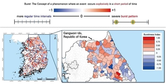
The burstiness index is made by scaling the temporal irregularities that appear in a certain phenomenon compared to other phenomena [31] and is derived based on the intervals of occurrences of events. The burstiness index is derived from the concept of “burst” [32], which refers to a phenomenon where an event occurs explosively in a short period of time. This concept is based on fat-tailed distributions such as power functions and log functions, rather than time series data that follow the Poisson distribution, and is assumed to follow that SOC mechanism [32,33]. The burstiness index is measured using the mean and standard deviation of the time between events as shown in Equation (7) [32,33].
where σ means the standard deviation of the time intervals between events, and μ means the average of the time intervals between events. The burstiness index appears as a value between −1 and 1. A value closer to −1 represents a time series phenomenon with more regular time intervals, a value closer to 0 represents a time series phenomenon that occurs more randomly, and a value closer to 1 represents a time series phenomenon that shows a more severe burst pattern [32,33].
Although the burstiness index has been used in many time series studies [34,35,36,37], they all examined temporal changes in characteristics without considering spatial locations. Therefore, Kim [8] proposed the local indicator of temporal burstiness (LITB) considering the spatial context. In the case of the proposed LITB, spatial units are set and the LITB is calculated for each of them. In this case, different LITB calculation formulas are applied depending on the boundary conditions as follows. The calculation formula for periodic boundary conditions (PBC), as shown in Equation (8), is used when the observed pattern is periodically repeated over time, and the calculation formula for open boundary conditions (OBC) as shown in Equation (9) is used when periodicity is not considered.
where n refers to total number of events and r refers to σ/μ [8]. As with the global burstiness index (Equation (7)), the LITB is derived as a value between −1 and 1. A value closer to −1 indicates that the time series phenomenon in the relevant spatial unit occurs at more regular time intervals, a value closer to 0 indicates that the time series phenomenon in the relevant spatial unit occurs more randomly, and a value closer to 1 indicates that the time series phenomenon in the relevant spatial unit shows a more severe burst pattern.
3. Construction of Forest Fire Occurrence Data and Method to Explore the Spatiotemporal Characteristics of Forest Fires
VIIRS active fire products are generated using 750 m and 375 m resolution data. The 750 m fire product provides continuity with MODIS 1 km fire product. The 375 m fire product uses the higher spatial resolution VIIRS channels I1-I5, complemented by channel M13, to detect and characterize sub-pixel active fires. It resembles the MOD14/MYD14 fire products of MODIS. Compared to MODIS 1 km fire detection products, the VIIRS 375 m fire product provides greater response over smaller fires, as well as improved mapping of the perimeters of large fires [38]. Therefore, the 375 m fire data were used in this study.
This study was largely conducted in two stages. First, the forest fire damage ledger data (Table 1) were combined with VIIRS-based forest fire occurrence data to produce forest fire occurrence data in the form of polygons [27]. In the case of small forest fires that could not be identified in the VIIRS data, buffers as large as the total damaged areas were given based on the information in the forest fire damage ledger to create data in the form of polygons. Then, the SOC mechanism of the forest fire data created was checked. Finally, in order to search for area where forest fires increase rapidly during certain period, the results of applying the LITB [8] to the domestic forest fire damage range data expressed in the form of polygon were discussed.
3.1. Construction of Forest Fire Damage Range Data
This study used forest fire damage ledger information on forest fires that occurred between 1 January 2003 and 31 December 2019 in Korea. The temporal range of the study was set to the first date of forest fire damage ledger information that could be collected by the Korea Forest Service. Since the construction of spatial data on forest fires through the forest fire damage ledger has limitations, the VIIRS image-based forest fire occurrence data (VNP14IMGTDL_NRT) provided by the Fire Information for Resource Management System (FIRMS) of EARTHDATA were also used to supplement the limitations [39]. The VIIRS image-based forest fire occurrence data collected were from 20 January 2012 to 31 December 2019, and were collected based on the date of the detection of the first forest fire in the VIIRS image-based forest fire occurrence data.
The VIIRS image-based forest fire occurrence data include the coordinates of the center points and imaging information of the pixels classified into forest fires among Suomi NPP satellite images. The forest fire classification algorithm follows the algorithm of Schroeder et al. [20]. The data classified as ‘High’ among the VIIRS forest fire data were used. Since the spatial resolution of the VIIRS image-based forest fire occurrence data is 375 m, the algorithm can detect forest fires of which the damaged area is about 14.06 ha or larger. However, forest fires of which the areas are about 1/10 of the detectable area can be detected because the intensity of the thermal wavelength of the pixel is clearly recorded so that the difference in statistical values between the places where the forest fire occurred and did not occur is clear [17]. Therefore, the condition for the forest fire damage area of the forest fire damage ledger that can be combined was set to at least 1.406 ha. The number of pieces of forest fire damage ledger information that could be combined with the VIIRS-based forest fire occurrence data according to this damage area condition was 191.
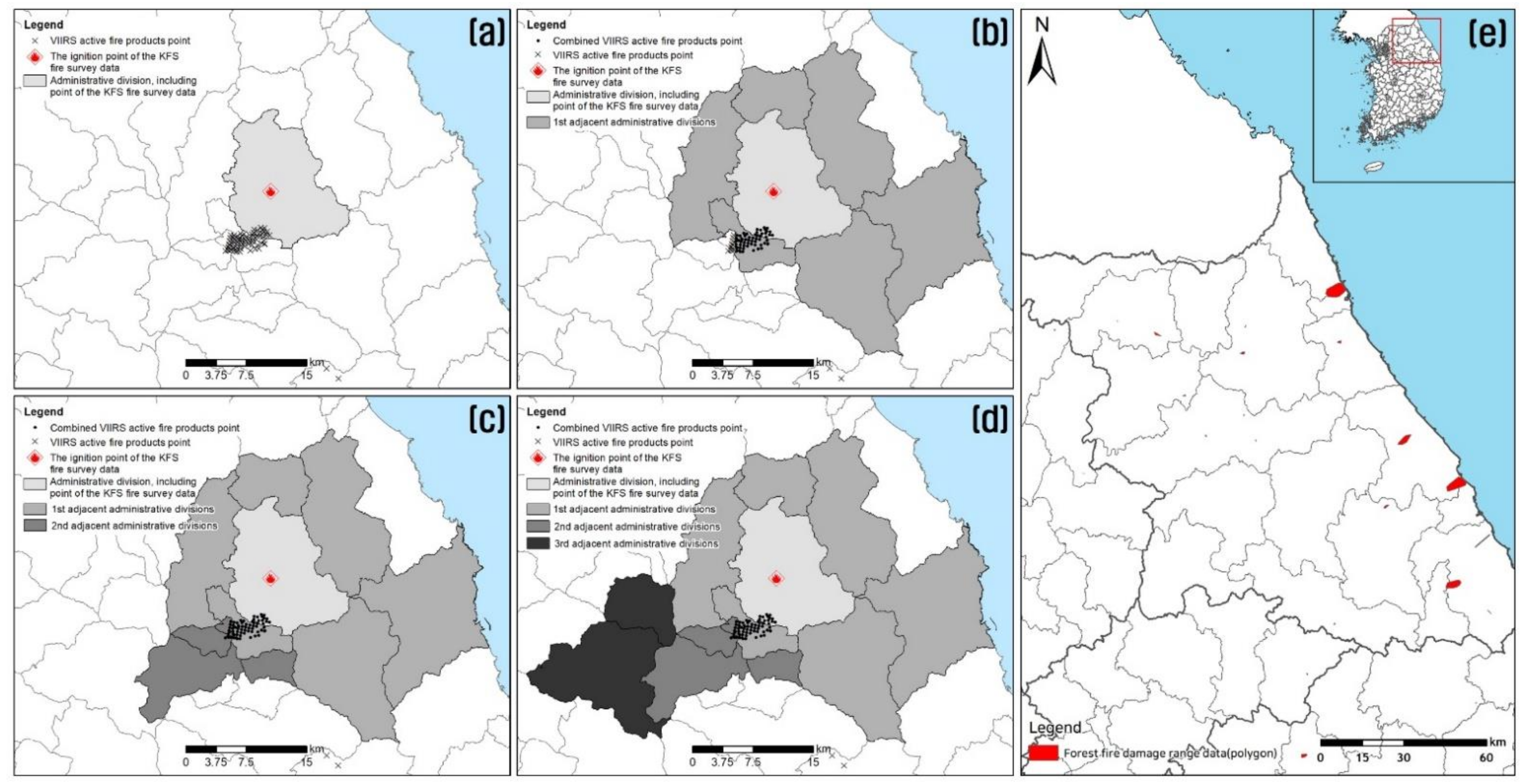
The process through which the VIIRS-based forest fire occurrence data, which are satellite image data, are combined with forest fire damage ledger information to construct forest fire damage range data in the form of polygons is as follows [27]. First, the dates and times of forest fire occurrences and forest fire extinguishment in the forest fire damage ledger were compared with the dates and times of the acquisition of the VIIRS image-based forest fire occurrence data to judge whether they match. Then, a combination analysis was performed with the matching data in four steps as shown in Figure 1. First, as shown in Figure 1a, an ignition point in the forest fire damage ledger was randomly selected. The “X” in Figure 1a is the VIIRS-based forest fire occurrence data corresponding to the forest fire occurrence time selected from the ledger. Second, as shown in Figure 1b, the VIIRS-based forest fire occurrence data found by searching the administrative division to which the point in the forest fire damage ledger belongs and adjacent administrative divisions that share a boundary line or boundary point with it were combined with the attribute information in the forest fire damage ledger. Then, as shown in Figure 1c, based on the administrative divisions for the combined VIIRS-based forest fire occurrence data, the administrative divisions that share a boundary line were searched secondarily and the VIIRS-based forest fire occurrence data found were combined with the attribute information in the forest fire damage ledger. By repeating this process, the search area was gradually expanded. Fourth, as shown in Figure 1d, when the searching is finished, the algorithm moves to the next fire point and start searching neighboring fire points. The same analysis was performed for the other ignition points in the forest fire damage ledger iteratively. Figure 1e shows the polygon fire map for Gangwon-do after iteration. By applying this method, combination analyses were conducted for the forest fire damage ledger and the VIIRS-based forest fire occurrence data.
Among the 191 cases of forest fires that meet the damage area condition in the forest fire damage ledger information, 84 cases were shown to have been combined with the VIIRS-based forest fire occurrence data. Among them, the cases of forest fires that have at least three points in the VIIRS-based forest fire occurrence data per case can be connected to construct forest fire damage range data in the form of polygons. The outermost points of 45 cases that could be combined were connected to construct forest fire damage range data in the form of polygons [25].
Meanwhile, since VIIRS images began to be processed in 2012 for the first time, 3145 forest fire data in the forest fire damage ledger from 2003 to 2011 used in this study could not be combined with VIIRS image-based forest fire occurrence data. In addition, in the case of each forest fire with two or fewer VIIRS-based forest fire occurrence data points combined with the forest fire damage area in the forest fire damage ledger, forest fire damage range data in the form of polygons could hardly be constructed. A total of 146 VIIRS-based forest fire occurrence data fell under the foregoing case. Therefore, for the two cases, buffers as large as the damaged area from the ignition point were given based on the forest fire damage ledger information to create forest fire damage range data in the form of polygons.
3.2. Method to Explore the Spatiotemporal Characteristics of the Burst of Forest Fire Occurrences in Korea
The daily frequencies of domestic forest fire occurrences can be drawn using domestic forest fire damage range data from January 2003 to December 2019, as shown in Figure 2. The frequencies of forest fire occurrences increase between March and May every year. From the foregoing, it can be seen that forest fire occurrences have seasonality in Korea, and this is thought to be attributable to the small precipitation amounts in winter and increase in climbers in spring. Therefore, in this study, detrended fluctuation analysis was performed with the daily forest fire occurrence frequency data to check whether forest fire occurrence time series data have long-term temporal correlations.
Next, the LITB was applied to domestic forest fire occurrences. In this case, as mentioned in the previous chapter, different LITB calculation formulas are applied depending on the boundary conditions. In this study, the periodic boundary condition is used since it is desirable when the pattern is expected be repeated or continued even in the temporal range beyond the observation period [8]. Therefore, for forest fires that have seasonality, calculating the LITB using the periodic boundary condition rather than the open boundary condition was judged to be favorable.
Meanwhile, since datasets summarized the times between forest fire occurrences as input data for the burstiness index, the LITB can be calculated only in areas where at least three forest fires occurred [8]. Therefore, areas where at least three forest fires were included within the boundaries of each administrative division were extracted for the LITB.
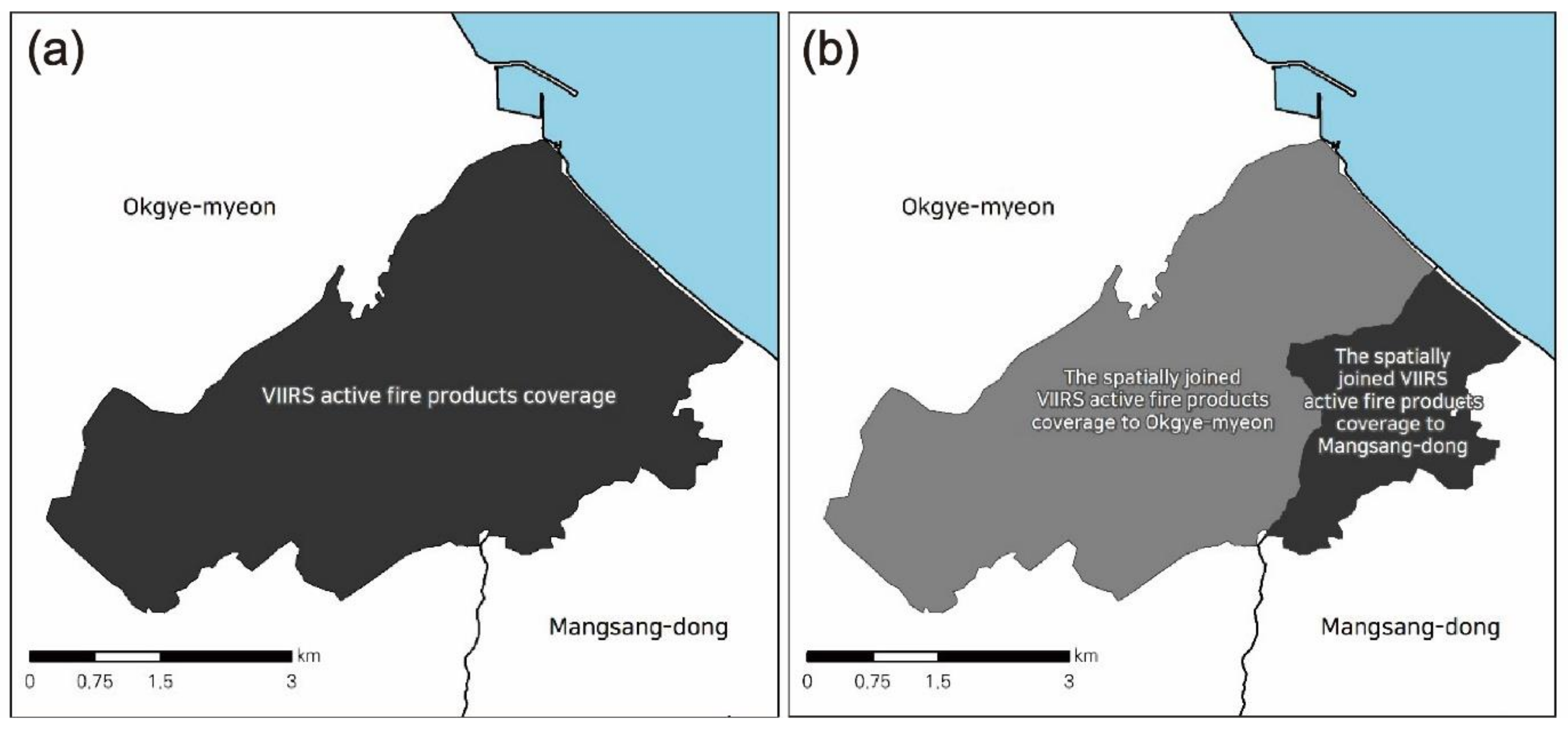
Spatial units should be set since the LITB is calculated for each spatial unit. The administrative divisions in forest fire damage range data were set as spatial units and LITBs were calculated for the units. In this case, since data in the form of polygons rather than points were used as input data to calculate LITBs, spatial join analysis was conducted for the forest fire damage range data. If a forest fire damage range appeared across two administrative divisions, such as Okgye-myeon and Mangsang-dong, as shown on the left side of Figure 3, the LITB was calculated regarding that a forest fire occurred in each administrative division as shown on the right side of Figure 3.
4. Results
4.1. Results of Detrended Fluctuation Analysis
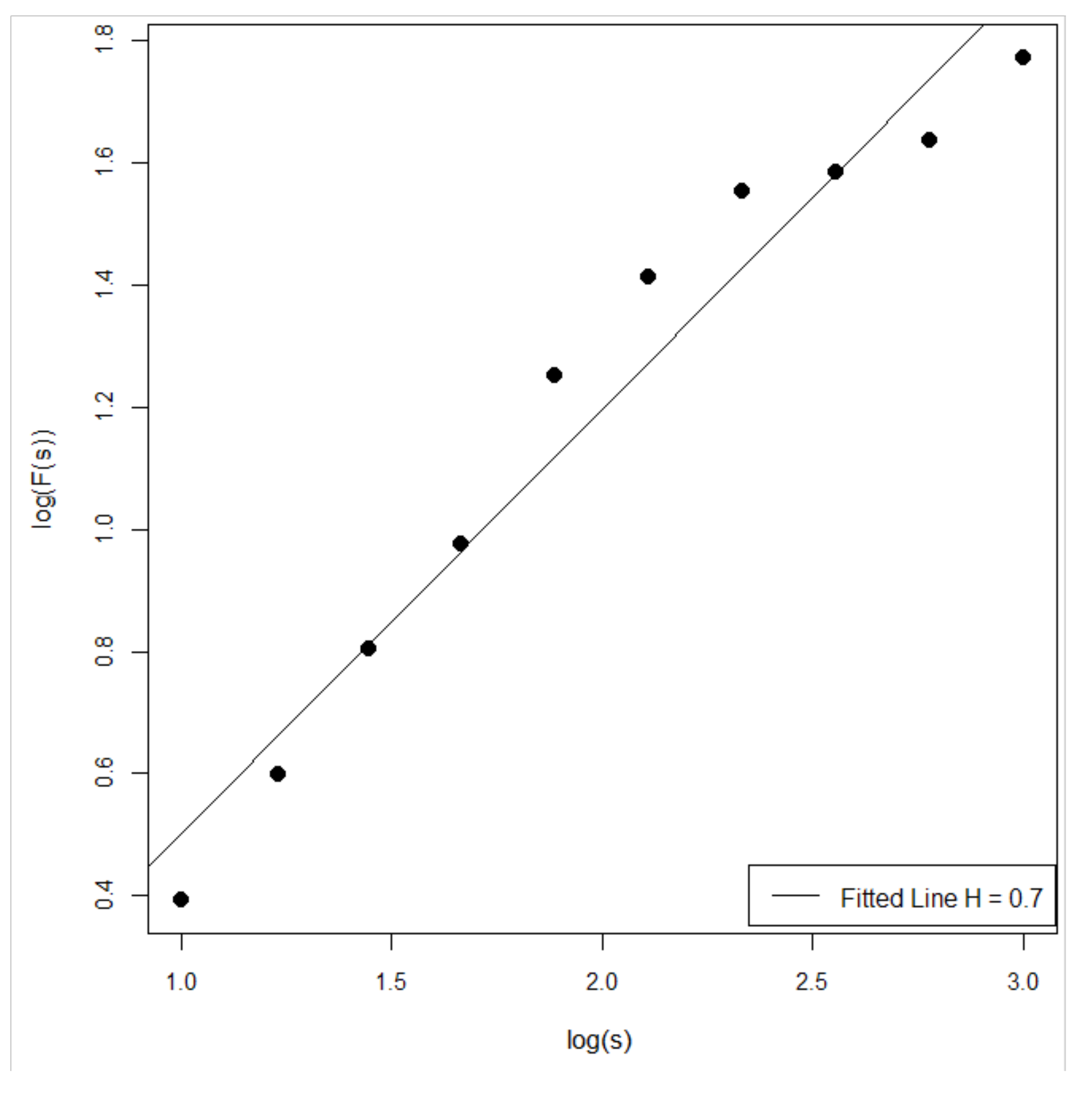
The results of the detrended fluctuation analysis are shown in Figure 4. The slope of the fitted line means the Hurst exponent. Since the calculated exponent is 0.7, the results mean that the Korean forest fire occurrence time series data from 2003 to 2019 show positive temporal correlations in the long term. This means that various factors that affect the occurrence of forest fires do not have an immediate effect, but slowly affect their occurrence over time. In other words, the Korean forest fire occurrence time series data show that the factors of the forest fire occurrence system interact and raise the system to a critical value over time, and a forest fire occurs when the critical state is exceeded. This can give positive or negative feedback for other forest fires that will occur in the future. Through the foregoing, it can be seen that forest fire occurrences in Korea follow the SOC mechanism.
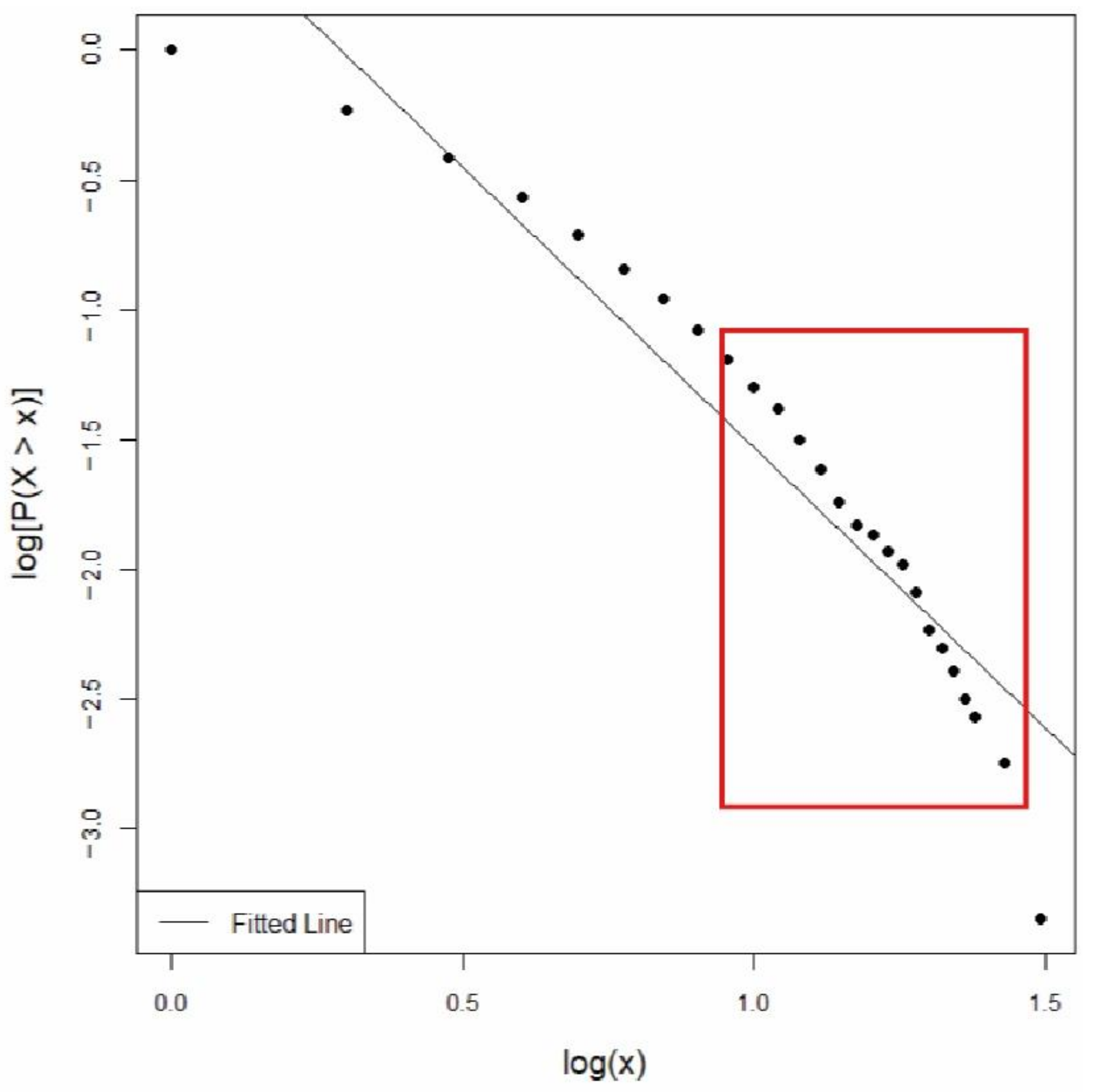
The time-series forest fire occurrence probability distribution that shows the SOC mechanism generally takes the form of a power law distribution. This is also called a fat-tailed distribution and has a characteristic that the probability of occurrence of an event is the highest at the minimum value rather than the average, unlike normal distribution [40]. In this study, to check whether the Korean time series forest fire occurrence phenomenon takes the form of a power law distribution, the complementary cumulative distribution function (CCDF) for the domestic forest fire occurrence time series data from 2003 to 2019 was shown with a log–log distribution as in Figure 4. The power exponent of the fitted line to the relevant time series distribution is 2.1612. The coefficient of determination for the power exponent of the fitted line is 0.9046, so it can be said that the fitted line explains the CCDF of the forest fire occurrence time series data well. Therefore, when Figure 5 is seen with the power exponent and the coefficient of determination, it can be seen that the forest fire occurrence time series data in Korea is in the form of a power law distribution.
4.2. Results of LITB Application
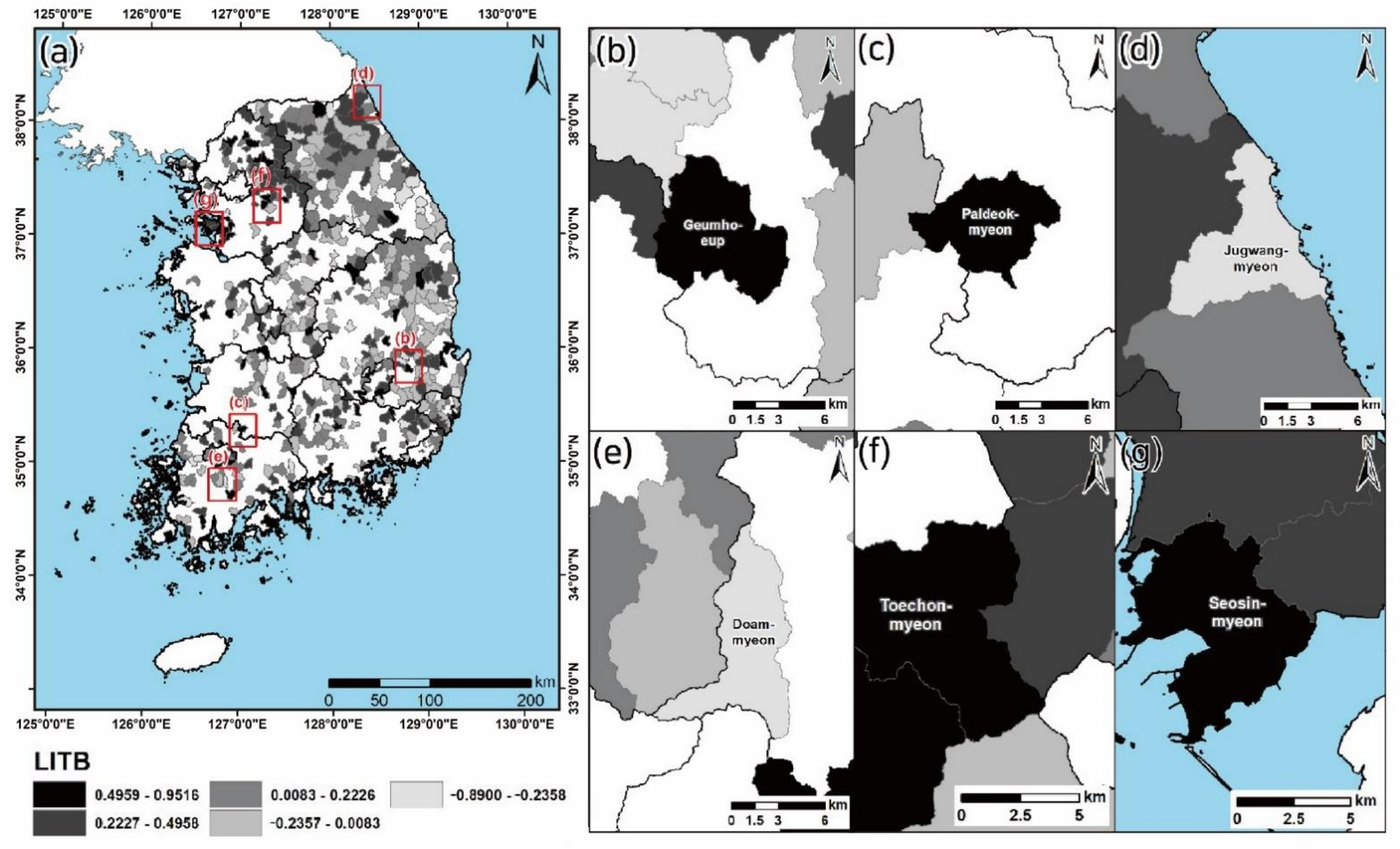
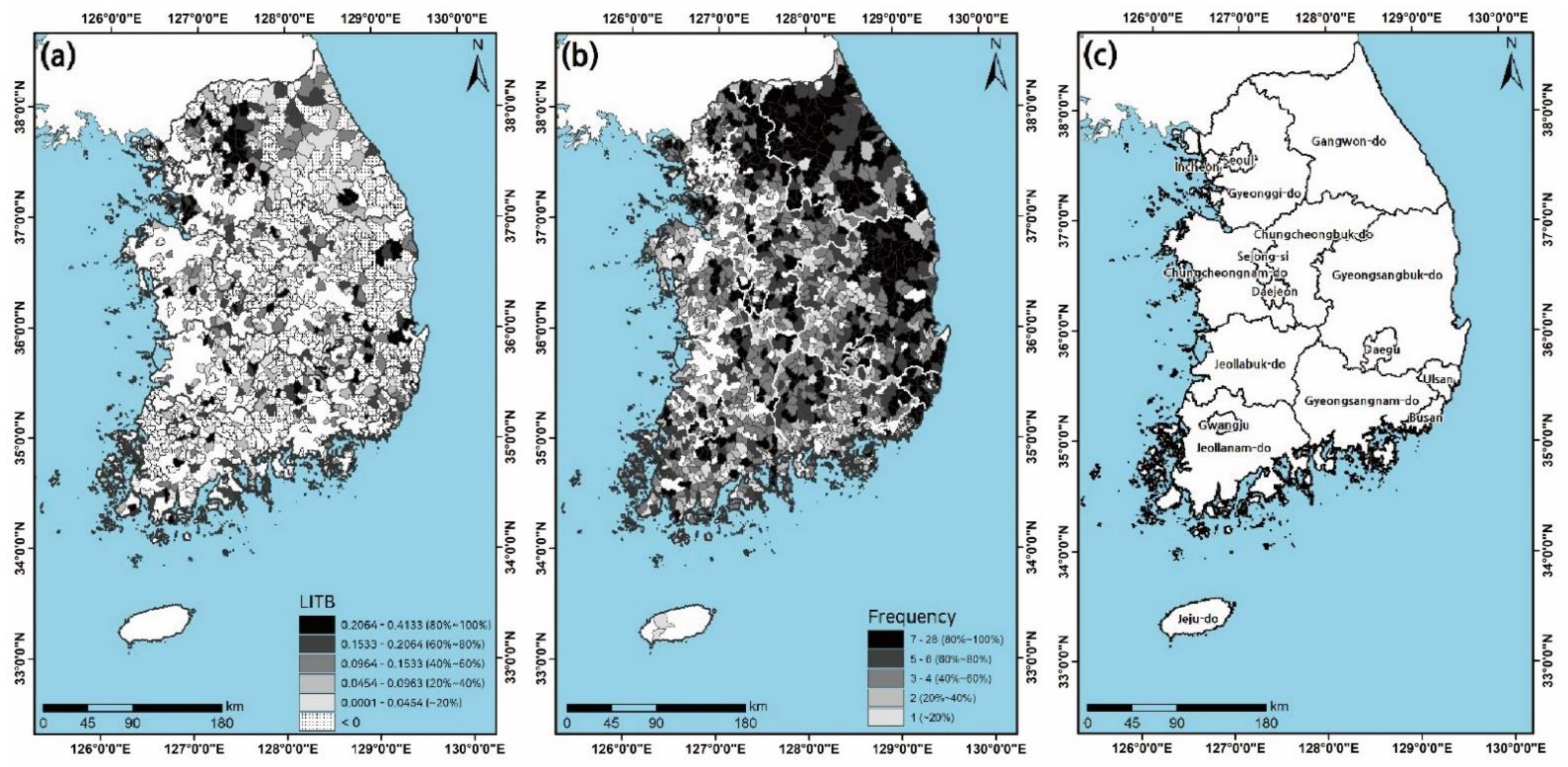
The results of derivation of LITBs for forest fire damage range data are shown in Figure 6. The LITBs in Figure 6 are only those of regions that were shown to be statistically significant at a significance level of 0.05 when the regions were restored and extracted by bootstrapping and tested for significance. The regions on the map where no color appears are regions that are not expressed because the LITB cannot be calculated or does not satisfy statistical significance. In addition, even if the local surge index can be calculated theoretically, if there are too few events in the unit space, the result may be overfitted. Therefore, this study attempts to analyze the results by selecting only areas that have more forest fires than the average number of forest fires by administrative divisions within the study period. Figure 6a shows the results of the entire study range, and Figure 6b,c show two regions with the highest LITB. Next, Figure 6d,e show two regions with the lowest LITB. Then, Figure 6f,g show two regions with the cycle of fires. In this study, the time series characteristics of forest fire occurrences according to LITBs were checked by examining two regions with the highest LITB and two regions with the lowest LITB as case areas.
The two regions with the highest LITBs are ‘Geumho-eup (0.9516) in Yeongcheon-si, Gyeongsangbuk-do’ and ‘Paldeok-myeon (0.9403) in Sunchang-gun, Jeollabuk-do’. The LITB is about 0.9 or more, which is a strong burst pattern, that is, the temporal pattern of the distribution of forest fires, appears somewhat irregular and can increase rapidly at a certain time. The detailed information on forest fire damage in the two regions is as follows. Most of Geumho-eup had forest fires between January and April 2009, and since then, forest fires have not occurred for a while, but have occurred in June 2017. The cause of the forest fire was due to the incineration of agricultural waste. In Paldeok-myeon, forest fires broke out from March to April 2005, and forest fires broke out again in February 2018. Wildfires were mainly caused by the ignition due to entrant’s negligence and the incineration of agricultural waste.
The two regions with the lowest LITBs are ‘Jukwang-myeon (−0.8900) in Goseong-gun, Gangwon-do’ and ‘Doam-myeon (−0.7264) in Hwasun-gun, Jeollanam-do’. The LITB of the two regions is around −0.8, which can be interpreted as forest fires occurring regularly compared to other regions. Looking at the time series of forest fires in the two regions, forest fires in Jukwang-myeon occurred every spring from 2015 to 2019. Doam-myeon is an area where forest fires steadily occur over the entire research range from 2003 to 2019, mainly in February and March. Looking at the causes of forest fires, most of them are caused by the misfire of entrants and visitors to the grave.
On the other hand, it is also possible to determine the cycle of forest fires by comparing the LITB with the distribution of forest fires. Figure 6f,g are case areas where the cycle is examined. Specifically, Figure 6f represents ‘Toechon-myeon (0.7605) in Gwangju-si, Gyeonggi-do’ and Figure 6g represents ‘Seosin-myeon (0.6724) in Hwaseong-si, Gyeonggi-do’. In Toechon-myeon, forest fires have not occurred for about 10 years since the forest fire in April 2004, but many small forest fires have occurred from 2014 to 2017. Most of the causes of the outbreak are due to the fire of visitors to the mountain or grave. Next, in Seosin-myeon, one case each occurred from 2003 to 2005, but no forest fire occurred for about 10 years. However, in 2015 and 2017, a number of forest fires occurred, and although the size of the forest fire was small, most of them were caused by incineration of garbage.
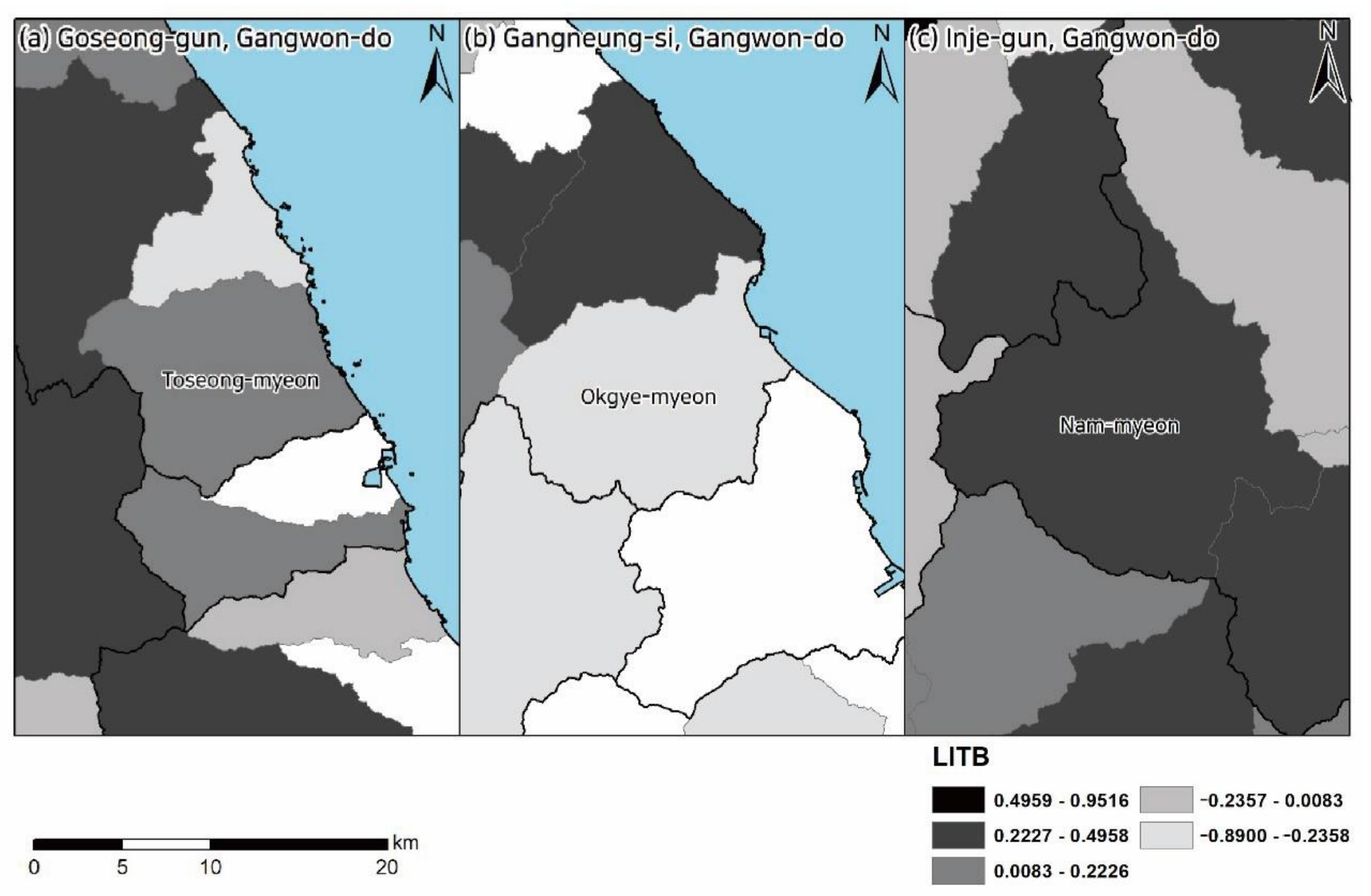
Among the catastrophic forest fires that occurred between 2003 and 2019, corresponding to the temporal range of this study, the forest fire that occurred in Gangwon-do in 2019 caused the most damage. The areas in Gangwon-do where forest fires occurred in 2019 (Figure 7) are ‘Toseong-myeon (0.0851) in Goseong-gun, Gangwon-do’, ‘Okgye-myeon (0.2600) in Gangneung-si, Gangwon-do’, and ‘Nam-myeon (0.2644) in Inje-gun, Gangwon-do’. Therefore, the LITBs of the forest fires that occurred in these regions between 2003 and 2019 and the time series characteristics of the forest fire occurrences were examined.
In the case of Toseong-myeon shown in Figure 7a, the LITB was 0.0851, which is a value close to zero. In fact, on reviewing the dates of forest fire occurrences, it could be seen that 11 forest fires occurred from 2003 to 2019, and the times of occurrence were irregular. However, after a medium-sized forest fire in an area of about 13 ha occurred in 2009, there was a large forest fire in an area of about 1266.62 ha in 2019, 10 years later. In the case of Okgye-myeon shown in Figure 7b, the LITB is somewhat weak at −0.2600, but the time series can be said to be somewhat regular. When the actual dates of forest fire occurrences are reviewed, it could be seen that forest fires occurred in spring at intervals of 2 or 3 years. In particular, after the occurrence of a large forest fire in an area of about 430 ha in 2004, a large forest fire in an area of about 1260 ha occurred again about 15 years later. Lastly, in the case of Nam-myeon shown in Figure 7c, it can be said that forest fires occur in a very weak burst pattern because the LITB is 0.2644. In fact, when the information on the damage due to forest fires in Nam-myeon was reviewed, it could be seen that forest fires steadily occurred every year, it was confirmed that it occurred intensively, especially in April and June.
5. Discussion
In order to examine whether forest fire occurrence time series data in Korea follow the SOC mechanism, this study examined whether the long-term temporal correlation and daily forest fire occurrence frequencies follow the power law distribution through DFA analysis. First, in the result of the DFA analysis, the derived Hurst exponent was 0.7, indicating that there is a long-term temporal correlation. In the case of the SOC mechanism, many factors in the system cause interactions by themselves to change the state of the system into a critical state. Therefore, the existence of a long-term temporal correlation means that certain factors are not immediately reflected in other phenomena, but gradually affect them, and that individual phenomena are temporally correlated. For example, a forest fire that occurred at a certain point in time may involve more frequent forest fires or may reduce forest fire occurrences through positive or negative feedback within the system. This process of feedback can be seen as interacting with each other and affecting future forest fires.
One of the important features of the power law is that looking at the normal distribution curve, the frequency of special events is very small, whereas in the power function graph, the frequency does not decrease rapidly. This phenomenon is called “Thick Tail” of the power law. In Figure 5, the CCDF was obtained using the daily forest fire occurrence frequency data and according to the results, the distribution formed a thick tail (right side box in Figure 5), and the explanatory power for the estimated power exponent was shown to be statistically significant. Therefore, it could be seen that the forest fire occurrence time series data follow the power law distribution, indicating that the forest fire occurrences are irregular in time series and that forest fires may burst on certain dates. In other words, it was identified that the daily forest fire occurrence frequencies shown in the forest fire damage ledger follow the SOC mechanism taking the form of a power law distribution.
As shown in Figure 6, the highest LITB regions are Geumho-eup (0.9516) and Paldeok-myeon (0.9403), and the lowest LITB regions are Jukwang-myeon (−0.8900) and Doam-myeon (−0.7264). The place where the LITB is high can be seen as an area with relatively strong temporal irregularities in forest fires compared to other regions. The place where the LITB is lower is the area where forest fires occur regularly compared to other regions. Thus, if the LITB is applied to forest fires, it is possible to compare the temporal irregularities of forest fires by unit space.
In previous studies on the occurrence of forest fires in Korea, studies on the frequency of forest fires were mainly conducted [41,42], but studies using LITB were not. Since November to May is the dry season in the Korean Peninsula, forest fires occur frequently, and the occurrence frequencies of forest fire were analyzed for local areas during this period to derive areas with high fire risk for resource allocation [43]. Therefore, the LITBs of forest fire occurrences in this study are compared with simple occurrence frequencies of forest fires to identify regions for allocating prevention resources. Figure 8 shows the results of comparison of the LITBs and simple occurrence frequencies in the data on forest fires that occurred in Korea between 2003 and 2019. In Figure 8, to compare the resultant LITBs with simple occurrence frequencies, the simple forest fire occurrence frequencies were divided into five percentile intervals, and LITBs values divided into five percentile intervals were expressed only when their values were positive.
As seen in Figure 8, the simple forest fire occurrence frequencies are high in Gangwon-do and Gyeongsangbuk-do, but LITBs are high in Gyeonggi-do. In particular, in Gangwon-do, since LITBs are shown to be low, temporal explosiveness can hardly be identified. This suggests that even where the frequencies of forest fires are similar, different patterns can be identified when the time-series distributions of occurrences are checked. In the case of Toechon-myeon (see Figure 6f) and Seosin-myeon (see Figure 6g), where LITBs were shown to be the highest earlier, it could be seen the forest fire occurrence frequencies in April and May sharply increased at intervals of about 10 years. Therefore, in the case of these two areas, it is desirable to concentrate on monitoring them for the prevention of forest fires in spring at normal times while making efforts to investigate the causes of concentrations of forest fires in April and May in detail to eliminate the causes.
6. Conclusions
In order to alleviate the spatial limitations of point data in the forest fire occurrence information in the forest fire damage ledger, this study constructed forest fire damage range data in the form of polygons by combining the ledger information with VIIRS-based forest fire occurrence data. In the case of the forest fires between 2003 and 2011 that were not combined with satellite images and small-scale forest fires in areas not exceeding 1.406 ha, forest fire damage range data were expressed in the form of polygons using damaged areas.
Using the data constructed, two kinds of analyses were conducted to examine the temporal characteristics of the distribution of forest fire occurrences. First, through detrended fluctuation analysis, whether time series forest fire occurrences have long-term temporal correlations according to the SOC mechanism, and whether the daily forest fire occurrence frequencies take the form of a power law distribution were checked. The value of the Hurst exponent derived through the analysis was 0.7, indicating that long-term temporal correlations exist. Therefore, it can be seen that the domestic forest fire occurrence system follows the SOC mechanism, in other words, forest fires that occurred in the past have long-term effects on the occurrence of forest fires in the future. Next, when the daily forest fire occurrence frequencies were expressed as a complementary cumulative distribution function, it was found that the distribution formed a thick tail, and when the estimated power exponent was checked, the results showed that the domestic forest fire occurrence time series were distributed in the form of a power law distribution. This suggests that there are temporal irregularities in the occurrence of forest fires in Korea, and that times when multiple forest fires occur during a day will appear someday without fail.
Second, based on the foregoing, LITBs were applied to the forest fire damage range data to examine how the temporal irregularities of forest fire occurrences appear by region. As a result of the analysis, Kumho-eup in Yeongcheon-si, Gyeongsangbuk-do and Paldeok-myeon in Sunchang-gun, Jeollabuk-do showed a high LITB, showing a pattern in which forest fires are concentrated at a specific time. When the dates and times of the forest fire occurrences in the two regions were checked, the forest fire occurrence frequency sharply increased at intervals of about 10 years. In addition, the spatial distribution of the LITBs and that of simple frequencies of forest fire occurrences were compared with each other and it was found that there were significant spatial differences between the simple occurrence frequencies and LITBs by region. Therefore, when allocating the necessary resources for forest fire management, if the burstiness index of forest fire occurrence and the times are grasped, a policy to allocate the resources more effectively can be established.
This study is meaningful in that it analyzed the temporal irregularities of forest fire occurrences in Korea through the characteristics of spatial distribution of LITBs. In particular, this study is meaningful in that it alleviated the spatial limitations of forest fire occurrence information in the form of points by combining the satellite image-based forest fire occurrence data with the forest fire damage ledger to construct and use the forest fire occurrence data in the form of polygons. Hereafter, if forest fire damage ledger information is gradually accumulated so that long-term time series information can be created, more in-depth time series analysis for forest fire occurrences can be performed by applying the SOC mechanism and LITB analysis used in this study.
Author Contributions
Each author’s contributions are as follows. Conceptualization, T.K. and J.C.; Methodology, T.K.; Software, T.K. and S.H.; Validation, T.K. and S.H.; Data Curation, T.K.; Writing—Original Draft Preparation, T.K.; Writing—Review and Editing, J.C.; Visualization, T.K. and S.H.; Supervision, J.C.; Project Administration, T.K.; Funding Acquisition, J.C. All authors have read and agreed to the published version of the manuscript.
Funding
This research was supported by a grant(2021-MOIS37-003) of Intelligent Technology Development Program on Disaster Response and Emergency Management funded by the Ministry of Interior and Safety (MOIS, Korea).
Institutional Review Board Statement
Not applicable.
Informed Consent Statement
Not applicable.
Data Availability Statement
Not applicable.
Conflicts of Interest
The authors declare no conflict of interest.
References
- Kumari, B.; Pandey, A.C. MODIS based forest fire hotspot analysis and its relationship with climatic variables. Spat. Inf. Res. 2020, 28, 87–99. [Google Scholar] [CrossRef]
- Ahmad, F.; Goparaju, L. A geospatial analysis of climate variability and its impact on forest fire: A case study in Orissa state of India. Spat. Inf. Res. 2018, 26, 587–598. [Google Scholar] [CrossRef]
- Korea Forest Service. Available online: https://www.forest.go.kr/kfsweb/kfi/kfs/frfr/selectFrfrStats.do?mn=NKFS_02_02_01_05 (accessed on 13 October 2021).
- Statistics Korea. E-National Index. Available online: https://www.index.go.kr/potal/main/EachDtlPageDetail.do?idx_cd=1309 (accessed on 13 October 2021).
- Bak, P.; Tang, C.; Wiesenfeld, K. Self-organized criticality. Phys. Rev. A 1988, 38, 364. [Google Scholar] [CrossRef]
- Song, W.; Wang, J.; Satoh, K.; Fan, W. Three types of power-law distribution of forest fires in Japan. Ecol. Model. 2006, 196, 527–532. [Google Scholar] [CrossRef]
- Lu, J.; Zhou, T.; Li, B.; Zhang, H.; Wu, C. Self-organized criticality in wildfire time series from China. Nat. Hazards Rev. 2017, 18, 04017014. [Google Scholar] [CrossRef]
- Kim, E.K. Local Indicators of Temporal Burstiness for Spatio-Temporal Event Analysis. Ph.D. Dissertation, Pennsylvania State University, State College, PA, USA, 12 December 2017. [Google Scholar]
- Zheng, H.; Song, W.; Wang, J. Detrended fluctuation analysis of forest fires and related weather parameters. Phys. A Stat. Mech. Its Appl. 2008, 387, 2091–2099. [Google Scholar] [CrossRef]
- Kato, A.; Thau, D.; Hudak, A.T.; Meigs, G.W.; Moskal, L.M. Quantifying fire trends in boreal forests with Landsat time series and self-organized criticality. Remote Sens. Environ. 2020, 237, 111525. [Google Scholar] [CrossRef]
- Lee, S.Y.; Kang, Y.S.; An, S.H.; Oh, J.S. Characteristic Analysis of Forest Fire Burned Area using GIS. J. Korean Assoc. Geogr. Inf. Stud. 2002, 5, 20–26. [Google Scholar]
- Kwak, H.B.; Lee, W.K.; Lee, S.Y.; Won, M.S.; Lee, M.B.; Koo, K.S. The Analysis of Relationship between Forest Fire Distribution and Topographic, Geographic, and Climatic Factors. In Proceedings of the GIS 2008 Joint Spring Conference on The Korean Society for Geospatial Information Science, Seoul, Korea, 13 June 2008; pp. 465–470. [Google Scholar]
- Lee, B.D.; Song, J.E.; Lee, M.B.; Chung, J.S. The Relationship between Characteristics of Forest Fires and Spatial Patterns of Forest Types by the Ecoregions of South Korea. J. Korean For. Soc. 2008, 97, 1–9. [Google Scholar]
- Kwak, H.B.; Lee, W.K.; Lee, S.Y.; Won, M.S.; Koo, K.S.; Lee, B.D.; Lee, M.B. Cause-specific Spatial Point Pattern Analysis of Forest Fire in Korea. J. Korean Soc. For. Sci. 2010, 99, 259–266. [Google Scholar]
- Lee, B.D.; Song, J.E. The Relationship between Spatial Patterns of Forest Distribution and Forest Fire Characteristics in the Regional Administrative Unit in Korea. Crisisonomy 2016, 12, 51–61. [Google Scholar] [CrossRef]
- Ahn, H.Y.; Lee, B.D.; Kwon, C.G.; Kim, S.Y. Identification of Fire-prone Areas Using Spatial Analysis of the Forest Fire Location Data. Crisisonomy 2017, 13, 95–104. [Google Scholar] [CrossRef]
- Giglio, L.; Descloitres, J.; Justice, C.O.; Kaufman, Y.J. An enhanced contextual fire detection algorithm for MODIS. Remote Sens. Environ. 2003, 87, 273–282. [Google Scholar] [CrossRef]
- Won, M.S.; Koo, K.S.; Lee, M.B. An Quantitative Analysis of Severity Classification and Burn Severity for the Large Forest Fire Areas using Normalized Burn Ratio of Landsat Imagery. J. Korean Assoc. Geogr. Inf. Stud. 2007, 10, 80–92. [Google Scholar]
- Kim, S.H. Development of an Algorithm for Detecting Sub-Pixel Scale Forest Fires Using MODIS Data. Master’s Dissertation, Inha University, Incheon, Korea, 2009. [Google Scholar]
- Schroeder, W.; Oliva, P.; Giglio, L.; Csiszar, I.A. The New VIIRS 375 m active fire detection data product: Algorithm description and initial assessment. Remote Sens. Environ. 2014, 143, 85–96. [Google Scholar] [CrossRef]
- Mallinis, G.; Mitsopoulos, I.; Chrysafi, I. Evaluating and comparing Sentinel 2A and Landsat-8 Operational Land Imager (OLI) spectral indices for estimating fire severity in a Mediterranean pine ecosystem of Greece. GISci. Remote Sens. 2018, 55, 1–18. [Google Scholar] [CrossRef]
- Oliva, P.; Schroeder, W. Assessment of VIIRS 375 m active fire detection product for direct burned area mapping. Remote Sens. Environ. 2015, 160, 144–155. [Google Scholar] [CrossRef]
- Hua, L.; Shao, G. The progress of operational forest fire monitoring with infrared remote sensing. J. For. Res. 2017, 28, 215–229. [Google Scholar] [CrossRef]
- Waigl, C.F.; Stuefer, M.; Prakash, A.; Ichoku, C. Detecting high and low-intensity fires in Alaska using VIIRS I-band data: An improved operational approach for high latitudes. Remote Sens. Environ. 2017, 199, 389–400. [Google Scholar] [CrossRef]
- Briones-Herrera, C.I.; Vega-Nieva, D.J.; Monjarás-Vega, N.A.; Briseño-Reyes, J.; López-Serrano, P.M.; Corral-Rivas, J.J.; Alvarado-Celestino, E.; Arellano-Pérez, S.; Álvarez-González, J.G.; Ruiz-González, A.D. Near Real-Time Automated Early Mapping of the Perimeter of Large Forest Fires from the Aggregation of VIIRS and MODIS Active Fires in Mexico. Remote Sens. 2020, 12, 2061. [Google Scholar] [CrossRef]
- NASA NPP. NPOESS Preparatory Project: Building a Bridge to a New Era of Earth Observations; NASA: Washington, DC, USA, 2011. [Google Scholar]
- Kim, T.H.; Choi, J.M. The Method of Linking Fire Survey Data with Satellite Image-based Fire Data. Korean J. Remote Sens. 2020, 36, 1125–1137. [Google Scholar]
- Peng, C.K.; Buldyrev, S.V.; Havlin, S.; Simons, M.; Stanley, H.E.; Goldberger, A.L. Mosaic organization of DNA nucleotides. Phys. Rev. E 1994, 49, 1685. [Google Scholar] [CrossRef] [Green Version]
- Hurst, H. Long-term storage capacity of reservoirs. Trans. Am. Soc. Civ. Eng. 1951, 116, 770–799. [Google Scholar] [CrossRef]
- Barunik, J.; Kristoufek, L. On Hurst exponent estimation under heavy-tailed distributions. Phys. A Stat. Mech. Its Appl. 2010, 389, 3844–3855. [Google Scholar] [CrossRef] [Green Version]
- Goh, K.I.; Barabási, A.L. Burstiness and memory in complex systems. EPL 2008, 81, 48002. [Google Scholar] [CrossRef] [Green Version]
- Barabasi, A.L. The origin of bursts and heavy tails in human dynamics. Nature 2005, 435, 207–211. [Google Scholar] [CrossRef] [PubMed] [Green Version]
- Karsai, M.; Jo, H.H.; Kaski, K. Bursty Human Dynamics; Springer: Berlin/Heidelberg, Germany, 2018; pp. 1–23. [Google Scholar]
- Karsai, M.; Kaski, K.; Barabási, A.L.; Kertész, J. Universal features of correlated bursty behaviour. Sci. Rep. 2012, 2, 397. [Google Scholar] [CrossRef] [Green Version]
- Kim, E.K.; MacEachren, A.M. An index for characterizing spatial bursts of movements: A case study with geo-located Twitter data. In Proceedings of the GIScience 2014 Workshop on Analysis of Movement Data, Vienna, Austria, 23 September 2014. [Google Scholar]
- Jo, H.H.; Perotti, J.I.; Kaski, K.; Kertész, J. Correlated bursts and the role of memory range. Phys. Rev. E 2015, 92, 022814. [Google Scholar] [CrossRef] [Green Version]
- Kim, E.K.; Jo, H.H. Measuring burstiness for finite event sequences. Phys. Rev. E 2016, 94, 032311. [Google Scholar] [CrossRef] [PubMed] [Green Version]
- NASA. Suomi NPP VIIRS Land. Available online: https://viirsland.gsfc.nasa.gov/Products/NASA/FireESDR.html (accessed on 13 October 2021).
- NASA. Fire Information for Resource Management System (FIRMS). Available online: https://earthdata.nasa.gov/earth-observation-data/near-real-time/firms (accessed on 13 October 2021).
- Kim, Y.K.; Kim, S.P.; Cho, H.S.; Sohn, H.G. A Study of Power Law Distribution of Korean Disaster and Identification of Focusing Events. J. Korean Soc. Civ. Eng. 2016, 36, 181–190. [Google Scholar] [CrossRef] [Green Version]
- Lee, M.; Lee, S.; Lee, J. Study of the Characteristics of Forest Fire Based on Statistics of Forest Fire in Korea. J. Korean Soc. Hazard Mitig. 2012, 12, 185–192. [Google Scholar] [CrossRef] [Green Version]
- Bae, M.; Chae, H. Regional Characteristics of Forest Fire Occurrences in Korea from 1990 to 2018. J. Korean Soc. Hazard Mitig. 2019, 19, 305–313. [Google Scholar] [CrossRef] [Green Version]
- Won, M.; Yoon, S.; Koo, G.; Kim, G. Spatio-Temporal Analysis of Forest Fire Occurrences during the Dry Season between 1990s and 2000s in South Korea. J. Korean Assoc. Geogr. Inf. Stud. 2011, 14, 150–162. [Google Scholar] [CrossRef] [Green Version]
Figure 1.
The process of combining the forest fire damage ledger and VIIRS-based forest fire occurrence data: (a) Select an arbitrary ignition point. (b) Search the administrative division to which the ignition point belongs and its neighboring administrative divisions to combine the VIIRS-based forest fire occurrence data found. (c) Additionally, combine the VIIRS-based forest fire occurrence data found while searching additional neighboring administrative divisions based on the combined VIIRS-based forest fire occurrence data. (d) When the searching is finished, the algorithm moves to the next fire point and start searching neighboring fire points. (e) The polygon fire map for Gangwon-do after iteration.

Figure 2.
Daily frequencies of forest fire occurrences (from 2003 to 2019).

Figure 3.
Spatial join process for a forest fire across the boundary of two administrative divisions: (a) forest fire damage range in Okgye-myeon and Mangsang-dong, (b) divisions of the forest fire damage range to calculate LITB.
Figure 3.
Spatial join process for a forest fire across the boundary of two administrative divisions: (a) forest fire damage range in Okgye-myeon and Mangsang-dong, (b) divisions of the forest fire damage range to calculate LITB.

Figure 4.
Log–log graph of daily occurrence frequency s and F(s) for Korean forest fire occurrence time series data.
Figure 4.
Log–log graph of daily occurrence frequency s and F(s) for Korean forest fire occurrence time series data.

Figure 5.
Log–log graph of the CCDF for domestic forest fire occurrence time series.

Figure 6.
Results of LITB analysis: (a) the entire study range, (b) the highest LITB region, (c) the region with the second highest LITB, (d) the region with the lowest LITB, and (e) the region with the second lowest LITB, (f) Toechon-myeon (0.7605) in Gwangju-si, Gyeonggi-do, (g) Seosin-myeon (0.6724) in Hwaseong-si, Gyeonggi-do.

Figure 7.
Results of analysis of LITBs of 3 regions in Gangwon-do: (a) Toseong-myeon (0.0851) in Goseong-gun, (b) Okgye-myeon (0.2600) in Gangneung-si, (c) Nam-myeon (0.2644) in Inje-gun.
Figure 7.
Results of analysis of LITBs of 3 regions in Gangwon-do: (a) Toseong-myeon (0.0851) in Goseong-gun, (b) Okgye-myeon (0.2600) in Gangneung-si, (c) Nam-myeon (0.2644) in Inje-gun.

Figure 8.
(a) LITBs, (b) frequencies of occurrence, and (c) administrative districts in the forest fire occurrence data.
Figure 8.
(a) LITBs, (b) frequencies of occurrence, and (c) administrative districts in the forest fire occurrence data.


Table 1.
Example of the forest fire damage ledger data.
| Occurrence Time | Time to Extinguish | Location_Office | Location_Sido | |
|---|---|---|---|---|
| 28 December 2019 10:28 | 28 December 2019 14:00 | Kyeonggi | Kyeonggi | |
| Location_Sigungu | Location_Eupmyun | Location_DongLi | Cause_Type | |
| Gwangju | Mok | Gi | ||
| Cause_Detail | Cause of Occurrence_Others | Damage Area_Total (Ha) | ||
| Accidental fire at the workplace | 0.33 | |||
Publisher’s Note: MDPI stays neutral with regard to jurisdictional claims in published maps and institutional affiliations. |
© 2021 by the authors. Licensee MDPI, Basel, Switzerland. This article is an open access article distributed under the terms and conditions of the Creative Commons Attribution (CC BY) license (https://creativecommons.org/licenses/by/4.0/).
Share and Cite
MDPI and ACS Style
Kim, T.; Hwang, S.; Choi, J. Characteristics of Spatiotemporal Changes in the Occurrence of Forest Fires. Remote Sens. 2021, 13, 4940. https://0-doi-org.brum.beds.ac.uk/10.3390/rs13234940
AMA Style
Kim T, Hwang S, Choi J. Characteristics of Spatiotemporal Changes in the Occurrence of Forest Fires. Remote Sensing. 2021; 13(23):4940. https://0-doi-org.brum.beds.ac.uk/10.3390/rs13234940
Chicago/Turabian StyleKim, Taehee, Suyeon Hwang, and Jinmu Choi. 2021. "Characteristics of Spatiotemporal Changes in the Occurrence of Forest Fires" Remote Sensing 13, no. 23: 4940. https://0-doi-org.brum.beds.ac.uk/10.3390/rs13234940
Note that from the first issue of 2016, this journal uses article numbers instead of page numbers. See further details here.