
Single Tree Classification Using Multi-Temporal ALS Data and CIR Imagery in Mixed Old-Growth Forest in Poland


Department of Geomatics, Forest Research Institute, Sękocin Stary, 3 Braci Leśnej Street, 05-090 Raszyn, Poland
*
Author to whom correspondence should be addressed.
Remote Sens. 2021, 13(24), 5101; https://0-doi-org.brum.beds.ac.uk/10.3390/rs13245101
Submission received: 4 November 2021
/
Revised: 29 November 2021
/
Accepted: 12 December 2021
/
Published: 15 December 2021
(This article belongs to the Special Issue Forest Monitoring in a Multi-Sensor Approach)
Abstract
:Tree species classification is important for a variety of environmental applications, including biodiversity monitoring, wildfire risk assessment, ecosystem services assessment, and sustainable forest management. In this study we used a fusion of three remote sensing (RM) datasets including ALS (leaf-on and leaf-off) and colour-infrared (CIR) imagery (leaf-on), to classify different coniferous and deciduous tree species, including dead class, in a mixed temperate forest in Poland. We used intensity and structural variables from the ALS data and spectral information derived from aerial imagery for the classification procedure. Additionally, we tested the differences in classification accuracy of all the variants included in the data integration. The random forest classifier was used in the study. The highest accuracies were obtained for classification based on both point clouds and including image spectral information. The mean values for overall accuracy and kappa were 84.3% and 0.82, respectively. Analysis of the leaf-on and leaf-off alone is not sufficient to identify individual tree species due to their different discriminatory power. Leaf-on and leaf-off ALS point cloud features alone gave the lowest accuracies of 72% ≤ OA ≤ 74% and 0.67 ≤ κ ≤ 0.70. Classification based on both point clouds was found to give satisfactory and comparable results to classification based on combined information from all three sources (83% ≤ OA ≤ 84% and 0.81 ≤ κ ≤ 0.82). The classification accuracy varied between species. The classification results for coniferous trees were always better than for deciduous trees independent of the datasets. In the classification based on both point clouds (leaf-on and leaf-off), the intensity features seemed to be more important than the other groups of variables, especially the coefficient of variation, skewness, and percentiles. The NDVI was the most important CIR-based feature.
1. Introduction
Tree species classification is important for a variety of environmental applications, including biodiversity monitoring [1], wildfire risk assessment [2], ecosystem services assessment [3], and sustainable forest management [4]. Mapping tree species through visual interpretation of aerial images by experts in combination with in situ measurements is labour-intensive, time-consuming, and costly. Moreover, the method is not applicable to large forest areas [5]. Accordingly, technological developments have influenced the possibility of mapping the forest species composition using remote sensing data.
Remote sensing data are divided into active and passive. Active sensors emit a signal from the sensor and, after reflection from the object, the signal is received and analysed. Active remote sensing includes light detection and ranging (LiDAR) and synthetic aperture radar (SAR) data. Passive sensors, on the other hand, use the analysis of signals emitted by the observed object. Multispectral and hyperspectral imagery are examples of passive remote sensing and have been used to classify tree species in recent decades [6,7,8,9,10]. However, in the development of solutions based on optical data, it has been found that multispectral and hyperspectral images have their own limitations [11]. For example, the same analysed tree species may have a different spectral reflectance in other parts of the forest depending on the sun-view geometry [8]. On the other hand, different tree species may have similar spectra, especially in a mixed pixel [12]. The main limitations of the pixel-based approach also include mixed pixels at the boundaries between classes [13]. With this in mind, and with the development of active sensors such as LiDAR, the use of airborne laser scanning (ALS) data shows great potential in the context of tree species mapping due to its ability to represent objects in a three-dimensional point cloud [14,15,16,17,18]. In contrast to multispectral and hyperspectral imagery, it is possible to extract the structural features of trees based on discrete returns or full-waveform ALS data [19,20]. Tree species differ in their leaf distribution and branching patterns under different conditions, resulting in different architectures that can be captured with ALS data [17].
The classification of tree species based on ALS data is mostly carried out by modelling differences in the structural and/or spectral characteristics of tree crowns [21]. In recent years, a large number of ALS-derived features have been proposed to enable the classification of tree species [15,22,23,24,25]. In general, the ALS features can be divided into two groups, namely structural and radiometric features. Structural features characterise the geometric structure of trees (e.g., tree height, crown volume, crown width, and crown shape), while radiometric features refer to specific echo parameters extracted from the received waveform (e.g., intensity metrics, backscatter cross-section, and distance between two waveform echoes) [26]. Structural features provide detailed information about the height characteristics of a tree based on the distribution of points within the crown. These features are effectively used in classifying tree species that have significant differences in leaf distribution characteristics along the crown height profile [27]. One factor that interferes with species-specific crown structure is the interspersion of tree crowns. Especially in dense stands, neighbouring trees can distort the spatial distribution of canopy points. The surroundings of a particular tree can have a decisive influence on its growth, and consequently neighbouring trees can alter its physical structure [28]. Therefore, the selection of an appropriate algorithm for the individual tree detection is also an important factor for the correct identification of specific tree species. Radiometric features provide information on the type, size, compactness, and density of the foliage [23,29,30]. The number of returns and the width of the echo depend on the quantity, distribution, and orientation of the scattering elements along the laser beam direction. All these characteristics can differ both within and between tree species and can therefore be useful for distinguishing tree species [17]. However, intensity values vary depending on flight altitude, atmospheric conditions, reflectivity of the target, and laser settings [31]. Therefore, some authors recommend performing a radiometric calibration of the ALS point cloud intensity, which improves the accuracy of the classification [25,32,33]. In recent years, the use of multispectral ALS in tree species classification has begun [34,35,36,37], and according to Amiri et al. [37], further research in this area should be considered to establish the capabilities of these data.
The successful identification of tree species is undoubtedly influenced by the timing of data acquisition. The appropriate periods for data acquisition are usually divided into two distinct seasons, namely when deciduous trees have leaves (leaf-on) and when deciduous trees are dormant (leaf-off). Therefore, physical changes in the crown structure are particularly relevant for deciduous tree species. To date, there are many studies dealing with the classification of tree species using leaf-on ALS dataset [24,27,28,38]. Fewer papers have focused on using only the leaf-off ALS dataset [39,40]. However, comparing or integrating ALS data from both seasons is becoming more common [5,17,18,41,42,43] (Table 1). More common studies using leaf-on data are associated with standard forest inventory practise because of the leafy condition and the ability to study various stand parameters during this period, although in some areas the leaf-off conditions are preferred. The reason for avoiding the leaf-off period is the much narrower window of time without foliage and bare ground in temperate and northern latitudes combined with the risk of snowfall [41]. Nevertheless, in the leaf-off period it is possible to have more reflections reaching deeper parts of the crown than in the leaf-on season, and there are more intermediate reflections from the inner part of the crown, providing more information about the vertical structure of the tree and its crown [44]. Therefore, using point clouds from both seasons has the tangible advantage of providing additional information about the vertical crown structure, more than using only one dataset based on discrete return or full-waveform ALS data [45].
In this study we used a fusion of three remote sensing (RM) datasets including ALS (leaf-on and leaf-off) and colour-infrared (CIR) imagery (leaf-on) to classify different coniferous and deciduous tree species, including dead class, in a mixed temperate forest in Poland. We used intensity and structural variables from the ALS data and spectral information derived from aerial imagery for the classification procedure. Our specific objectives were as follows: (1) to evaluate and compare species classification accuracies of all variants contained in the data integration, (2) to identify the most appropriate period of data acquisition for the classification of individual tree species, and (3) to investigate the most important metrics for tree species classification.
2. Materials and Methods
2.1. Study Area
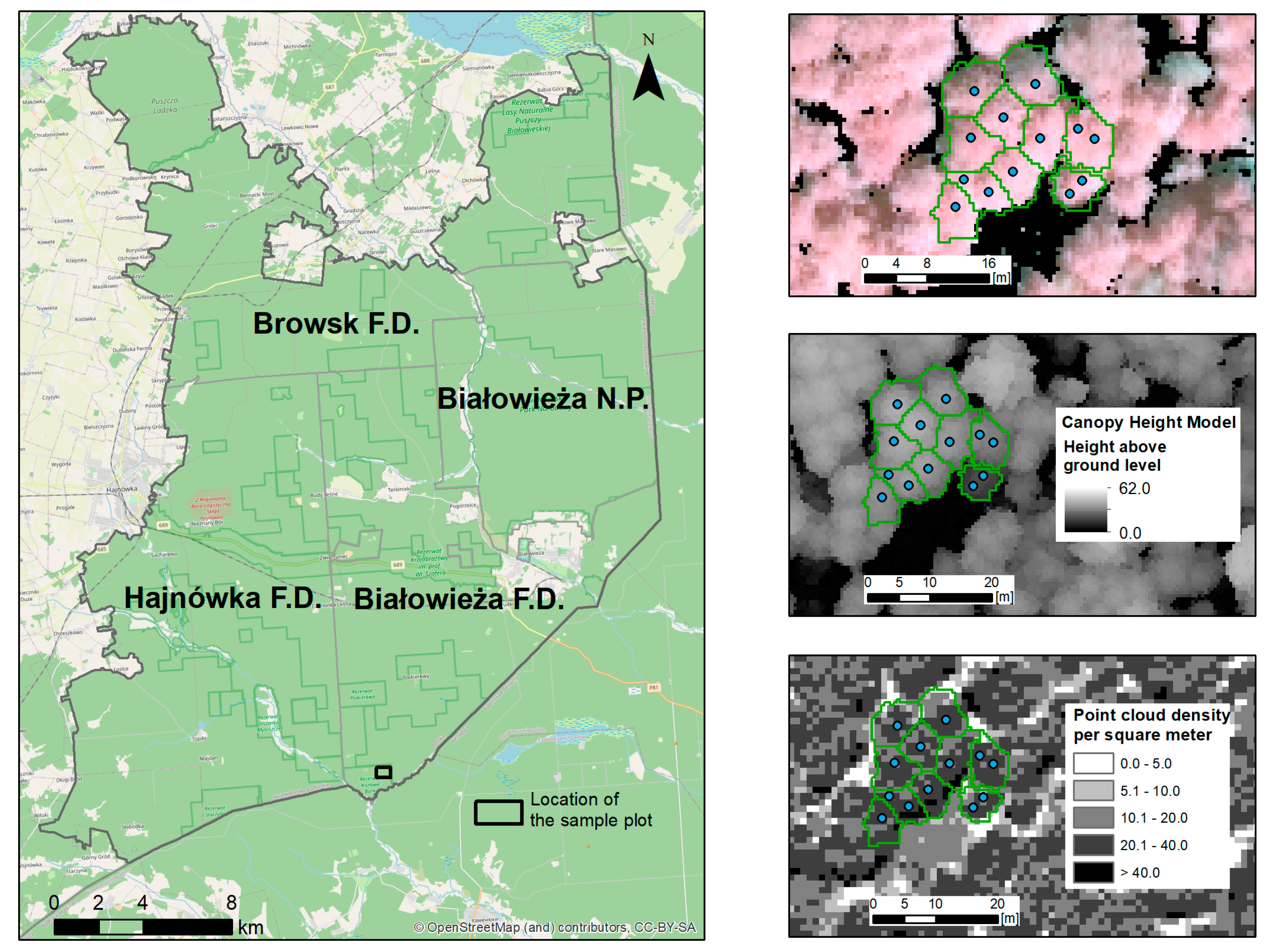
The Białowieża Forest (BF) is a large forest complex located on the border between Poland and Belarus (52°45′29″N, 23°46′8″E). A part of the BF has retained its original character, thanks to the protection lasting for several centuries. The Polish part of BF covers approx. 62,000 ha, of which 10,500 ha is a national park; nature reserves cover about 12,000 ha, while the remaining forests are about 39,500 ha (Figure 1).
The area of BF comprises a lowland forest complex, characteristic of the Central European mixed forest ecoregion. The area is of exceptional importance for nature conservation due to its area of old-growth forests covering large intact areas where natural processes occur. Taking into account the upper layer of the tree stand, the share of individual species in the Białowieża National Park in 2015 was 20% alder (Alnus glutinosa (L.) Gaertn.), 16% hornbeam (Carpinus betulus L.), 15% spruce (Picea abies (L.) H. Karst), 13% pine (Pinus sylvestris L.), 12% lime (Tilia cordata Mill.), 9% oaks (Quercus robur L. and Quercus petraea (Matt.) Liebl.), 6% birches (Betula pendula Roth., and Betula pubescens Ehrh.), and 9% other, while in the BF part outside the national park there was 23% spruce, 19% alder, 17% pine, 8% oaks, 8% hornbeam, 7% lime, 7% birches, and 11% other [46].
2.2. ALS Data and CIR Aerial Images
The leaf-on ALS dataset was acquired on 2–5 July 2015, while data from the leaf-off season was acquired 25 and 27 November 2015 and 6–7 December 2015. Both point clouds were acquired using the Riegl LMS-Q680i scanner (wavelength 1550 nm) integrated in a full-waveform laser scanning system. Simultaneously, in the leaf-on season, CIR images were obtained. This allowed the provider to assign spectral values to each point from the point cloud. The point density was around 11 points/m2. The flying altitude was approximately 500 m above ground. A total of 135 individual flight lines were recorded with 40% strip overlap. ALS leaf-off data were used to generate the digital elevation model (DEM) and ALS leaf-on data to generate the digital surface model (DSM) with a 0.5 m resolution. Forty-five points on logs were measured using RTK to verify that the points were classified as ground that was included in the generation of the DTM. This comparative procedure is expressed as an RMSE (root mean square error) value of 0.08 m. These models allowed the calculation of a normalized digital surface model (nDSM) [47] on which the segmentation process of individual trees was based. A commonly used marker-controlled watershed segmentation algorithm was chosen for the work. Individual trees and crowns were detected using the method proposed by Stereńczak et al. [48], who attempted to parameterise the segmentation into three height ranges (h ≤ 25 m; 25 m < h ≤ 35 m; h > 35 m). For each height range, the canopy height model is filtered with different settings assigned during the automatic optimisation for each height range. After the filtration process, hierarchical segmentation was performed, starting from the top layer of the tree canopies using a pouring algorithm. Subsequently, the resulting segments were adjusted in a five-step procedure. To obtain a more accurate classification, it is necessary to calibrate the intensity values to reduce the influence of various factors that affect these values, such as the range from the sensor. In our study, the radiometric calibration of the ALS point cloud intensity was performed using a simplified model described in Korpela et al. [32].
CIR aerial images were collected using an UltraCam Eagle Camera. CIR images were acquired from 3040 m, with 0.2 m ground sampling distance (GSD). In total, 1372 images were taken. Coverage between them was 90%/40% along-track/cross-track overlap, respectively. Each point in the ALS data contained spatial information from aerial imagery projected orthogonally to be able to assign CIR values. The acquired images were used in the process of point cloud colourization.
2.3. Field Measurement
Field data were collected from July to the end of October 2015. A total of 685 circular sample plots of a 12.62 m radius were measured. Sample plots were distributed throughout the BF. During the fieldwork, a large number of tree-related characteristics were recorded: tree species, tree height, crown length, and diameter at breast height. In addition, for each tree, its visibility from above was determined, i.e., the possibility of its registration on photogrammetric data. The centres of each plot were measured using real-time kinematic (RTK) or a static-mode, geodetic-class global navigation satellite systems receiver. The SD = 0.096 m was the result of the differential pre-processing of row GNSS data. We assumed a similar or better precision for the RTK fix mode, which was much less frequently used due to the dense forest in which the measurements were carried out. Based on the relationship between the tree and sample centre (distance and azimuth), the position of each tree was calculated.
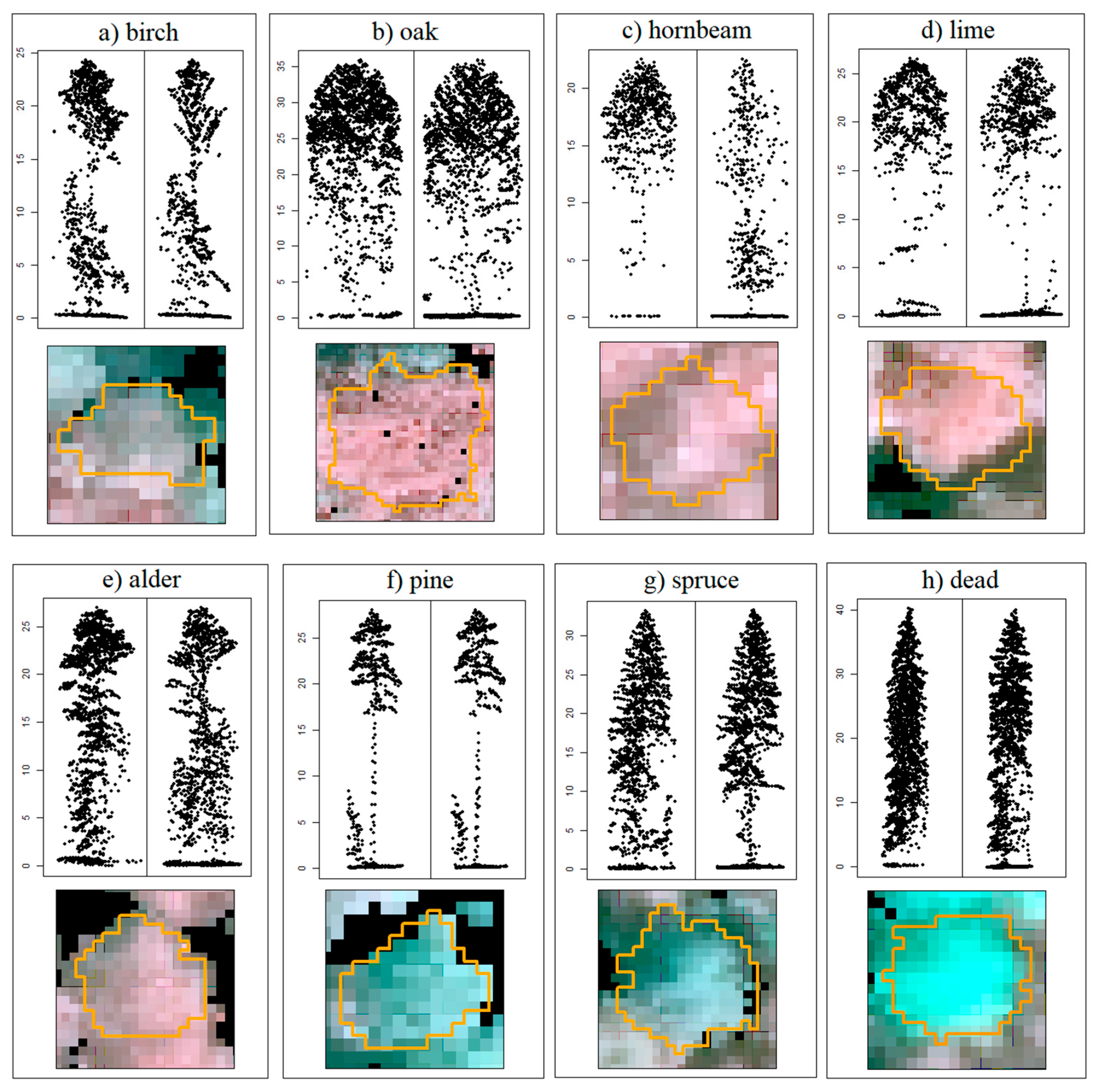
The seven tree species dominant in the Białowieża Forest were considered in the tree species classification: birch (Betula spp.), oak (Quercus spp.), hornbeam (Carpinus betulus L.), lime (Tilia cordata Mill.), alder (Alnus glutinosa Gaertn.), pine (Pinus sylvestris L.), and spruce (Picea abies (L.) H. Karst). In addition, a class of dead trees was selected, containing mainly dead spruce trees. The number of sample trees were selected based on their estimated percent coverage in the study area. A total of 1230 reference trees were selected, subdivided by species (Table 2). Selected trees varied in height and crown width in order to build a model with the highest possible variability. Examples of point cloud cross-sections from both seasons and CIR images for individual tree species are shown in Figure 2.
2.4. Extracting ALS and CIR Features
Classification features were derived from height measurements of ALS describing vertical crown structure (“structural features”), from the intensity distribution of ALS (“intensity features”), and from the RGB attribute of the point cloud (“CIR features”). The intensity features were computed for the first echoes (first of many and single echoes). Since the purpose of our work is to distinguish individual trees in the canopy as reliably as possible, the ALS features (structural and intensity) and CIR features were calculated only for points above half the height (H = Hmax/2) of a given segment [25], except for the features marked as “additional” in Table 3. A description of all the features used in the study can be found in Table 3.
All features were calculated for ALS point clouds and CIR attributes within segments (the results of the single tree detection procedure). The classification was based on different datasets, and the explanation of the coded symbols on the basis of which each variant was defined is given in Table 4.
For example, CIR_ALSSW means that a variant with features derived from the ALS point cloud from both seasons (SW) and CIR aerial images were used, while W_CanRR means the canopy relief ratio calculated from the point cloud from the leaf-off season.
2.5. Classification Strategy
The classification was conducted using the random forests (RF) algorithm [49]. To avoid overfitting the classification model, a 5-fold cross-validation was performed, repeated 20 times, and the mean classification accuracy indices for each classifier were determined. The classification and optimization processes were performed using the Caret package in R [50].
The random forests algorithm [49] used in the study is a further development of the classification trees [51]. The algorithm belongs to the ensemble classification methods. Each tree is generated using the bagging method. A large number of trees are generated and the classification result is obtained as a voting result. When a training set contains N cases, N cases are selected randomly but with a replacement to create a tree. The remaining cases (about 37% of the total sample size) are called out-of-bag (OOB) samples and are used for validation. At each node of a tree, m variables are randomly selected from M (the total number of variables) and used to find the best split. The classification algorithm is implemented in the randomForest package for R [52]. The following parameter settings for RF were used in each classification: 500 decision trees were created, with the number of predictors randomly selected at each partitioning equal to sqrt(M).
2.6. Accuracy Assessment and Statistical Analysis
The accuracy of the classifications was evaluated using an error matrix and the following indices: overall accuracy (OA), kappa coefficient (κ), producer accuracy (PA), and user accuracy (UA) [53,54]. Additionally, F1-score was calculated for each class according to the following formula:
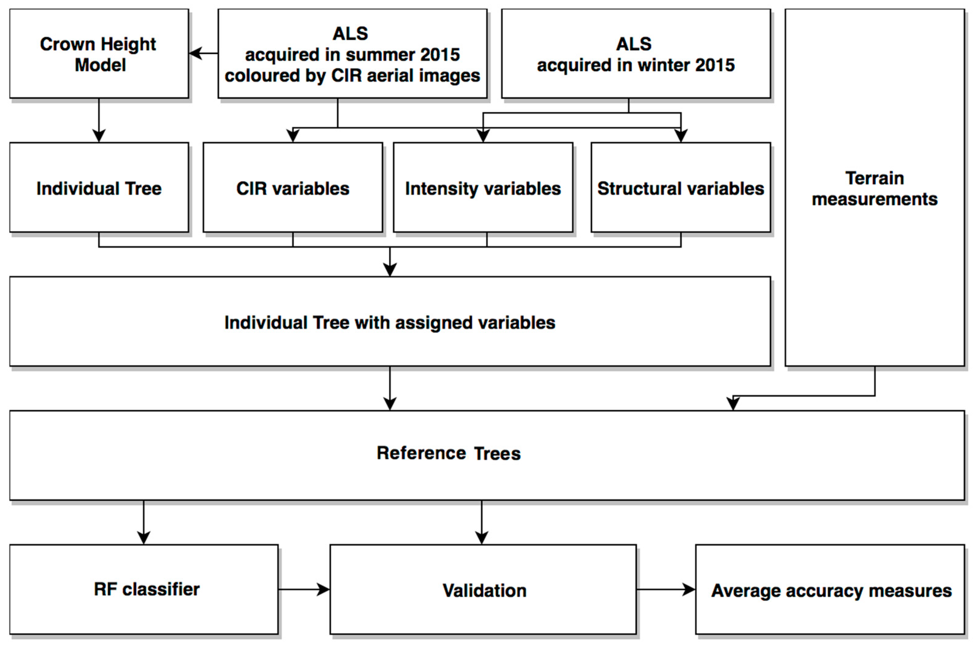
The importance of the variables for each iteration was recorded and the mean importance measure of each feature was calculated to select the best predictors. In addition, the discrimination between classes was tested by the Kruskal–Wallis test. McNemar’s test was used to determine if there were statistically significant differences between pairs of classification variants with the different predictor settings [55]. For all statistical tests, the significance level was set at α = 0.05. The methodological framework developed in this study for classifying individual trees is shown in Figure 3.
3. Results
3.1. Classification Results
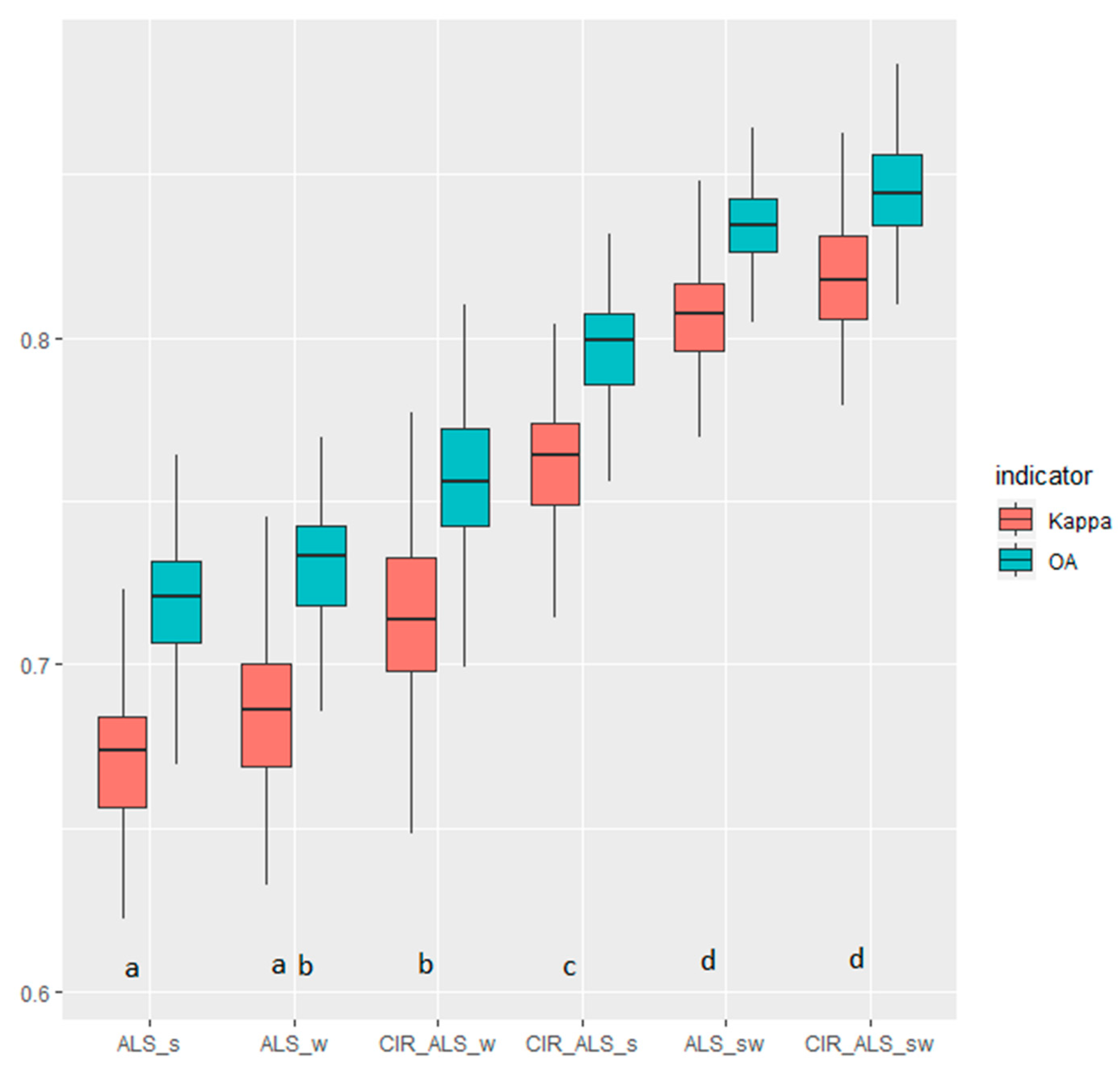
In general, we can state that all classification results, with different combinations of ALS features and CIR, result in high accuracy (Figure 4). The highest levels of accuracies were obtained for classification based on both point clouds and including image information (CIR_ALSSW); mean values of overall accuracy and kappa were equal to 84.3% and 0.82, respectively. Slightly worse, though not statistically significant (McNemar’s test, p > 0.05) classification results were obtained for both point clouds (ALSSW); the decrease of 0.01 in the kappa coefficient and 1 percentage point in overall classification accuracy were noted without CIR variables (Figure 4). Leaf-on and leaf-off ALS point cloud features alone produced the lowest accuracies with no statistically significant difference (McNemar’s test, p > 0.05). The variant ALSs turned out to be the worst option and resulted in OA = 72.1% and κ = 0.67. Image information (CIR variables) improved classification accuracies when comparing classification based on the leaf-on cloud alone, with an increase of 0.09 for the kappa coefficient and 8 percentage points for overall accuracy. CIR variables increased the overall accuracy from 73.2% (leaf-off) to 75.8% (leaf-off with CIR) as well as the kappa coefficient from 0.69 to 0.72, respectively. However, the difference between both variants was not statistically significant (McNemar’s test, p > 0.05).
It is worth noting that the classification results were distinguished by their low variability. The standard deviation (STD) of the overall accuracy and kappa for all variants was less than 2% and 0.027, respectively.
3.2. Species Classification
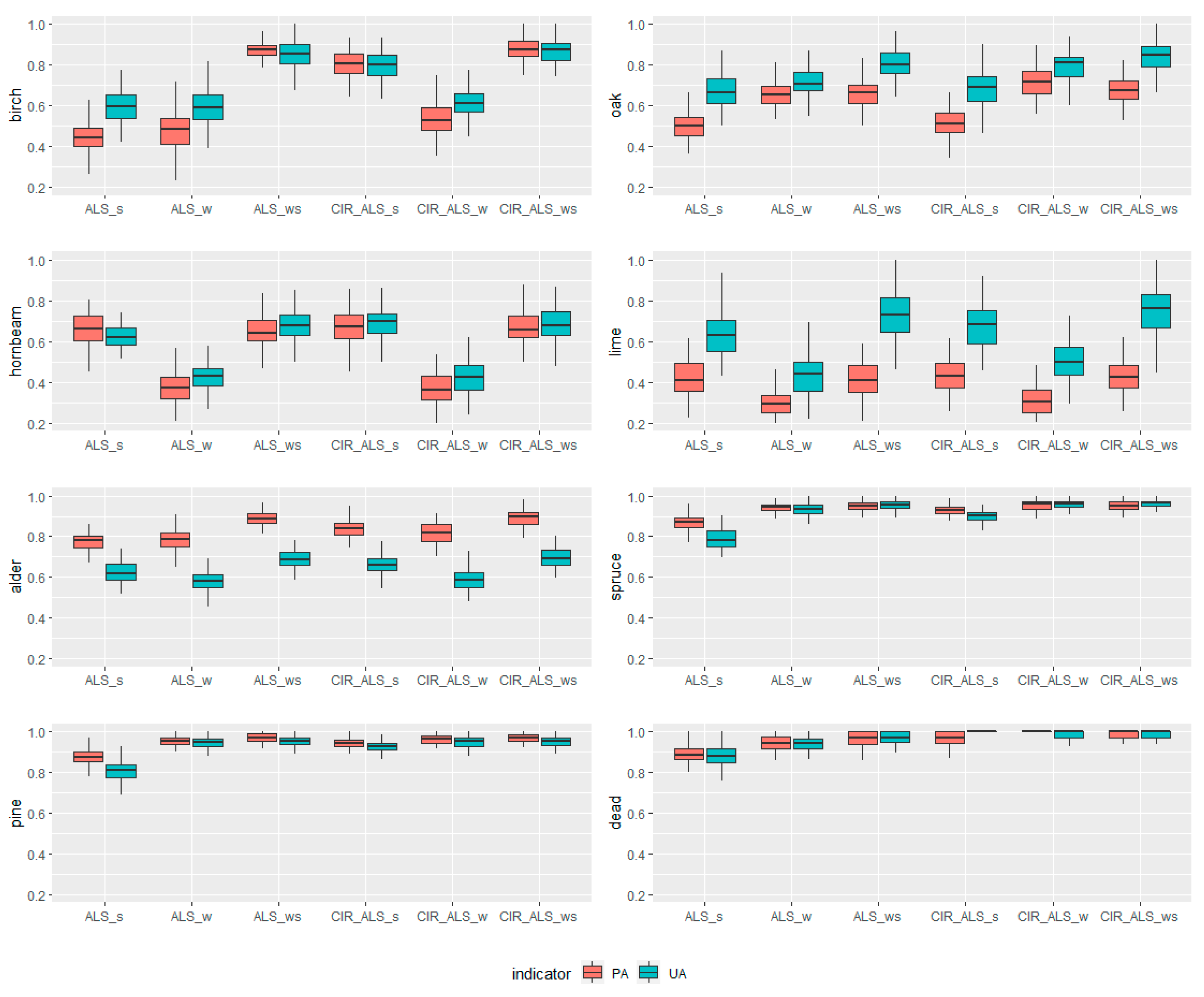
Classification accuracy varied between species (Figure 5). Regardless of the variant, coniferous trees (living and dead) were always classified with the higher accuracy (≥79% for both PA and UA among all variants) than deciduous (0.43 ≤ UA ≤ 0.87; 0.28 ≤ PA ≤ 0.89). Among all the classes, dead spruce was best classified: it only mixed slightly with living spruce.
Statistically significant differences between leaf-on and other variants were noticed for spruce, pine, and dead trees. Additionally, no significant differences were noticed for all variants apart from leaf-on acquisition (UA/PA ≥ 0.9), for which accuracies were the worst (UA/PA ≤ 0.9). In the leaf-on season, conifers blended with birch and additionally alder fell into the conifers.
Among deciduous trees, the lowest classification accuracies were noticed for lime (0.44 ≤ UA ≤ 0.75; 0.28 ≤ PA ≤ 0.43) independent of the analysed datasets. Especially in leaf-off season, lime was often classified as alder or hornbeam. McNemar’s test did not indicate significant differences between each pair of the rest of the acquisition variants (Table 5).
Quite good classification results were obtained for alder (0.58 ≤ UA ≤ 0.70; 0.77 ≤ PA ≤ 0.89). The worst accuracies for that species were noticed for both point clouds alone (UA = 0.58–0.63, PA = 0.77–0.78). McNemar’s test did not indicate significant differences between each pair of stacked acquisition results (CIR_ALSW, CIR_ALSS, CIR_ALSSW, ALSSW) (Table 5). Generally, it can be stated that alders were mixed with birches, although other deciduous species were also often classified as alder. Additionally, in the leaf-on season, it happened to be classified as spruce or pine.
Similar to alder, significantly lower classification results for leaf-on and leaf-off seasons alone (UA = 0.59–0.60, PA = 0.45–0.47) than the rest of the variants were noticed for birch. The best results for that species were obtained for the three combined datasets (UA = 0.87, PA = 0.88) with no significant differences with the combined leaf-on and leaf-off datasets (UA = 0.85, PA = 0.87). Regardless of the variant, birch was mixed with other deciduous trees—with conifers in the leaf-on season and other deciduous trees under leaf-off acquisition.
The worst classification results for oak were obtained based on the leaf-on ALS point cloud alone (UA = 0.67, PA = 0.50) and the best accuracies were based on both point clouds and including image information (CIR_ALSSW) (UA = 0.84, PA = 0.68) with no significant differences with ALSW, CIR_ALSW, and ALSSW variants (0.71 ≤ UA ≤ 0.80; 0.65 ≤ PA ≤ 0.72). Oak in general only mixed with deciduous (except birch), doing so the most under leaf-on acquisition.
In the case of hornbeam, the results obtained for leaf-off and leaf-off with CIR data (UA = 0.43, PA = 0.37) were statistically significantly lower than the other variants (0.65 ≤ UA/PA ≤ 0.68), for which McNemar’s test did not indicate significant differences between each pair of acquisition results (Table 5). Hornbeam, like oak, did not mix with coniferous. It mixed with all other deciduous, especially under leaf-off acquisition.
F1-scores of the species classification results can be used for ranking possible data combinations. Additionally, McNemar’s test determined if there were statistically significant differences between pairs of classification variants with the different predictor settings. Table 5’s results indicate that the leaf-off season was more favourable for conifers and oak, while hornbeam and lime exhibited better results in the leaf-on season. The combination of both point clouds was favourable for birch and alder. Image information (CIR variables) significantly improved classification accuracy when comparing classification based on the leaf-on cloud alone for birch and conifers.
3.3. Predictors Importance
The most important features for each variant for tree species classification based on measurements provided by the RF algorithm were presented in Table 6. Generally, in the classification based on both point clouds (leaf-on and leaf-off), the intensity features appeared to be more important than the other groups of variables, in particular the coefficient of variation, skewness, and percentiles. In the classification based on point cloud with CIR features, NDVI was among the most important predictors.
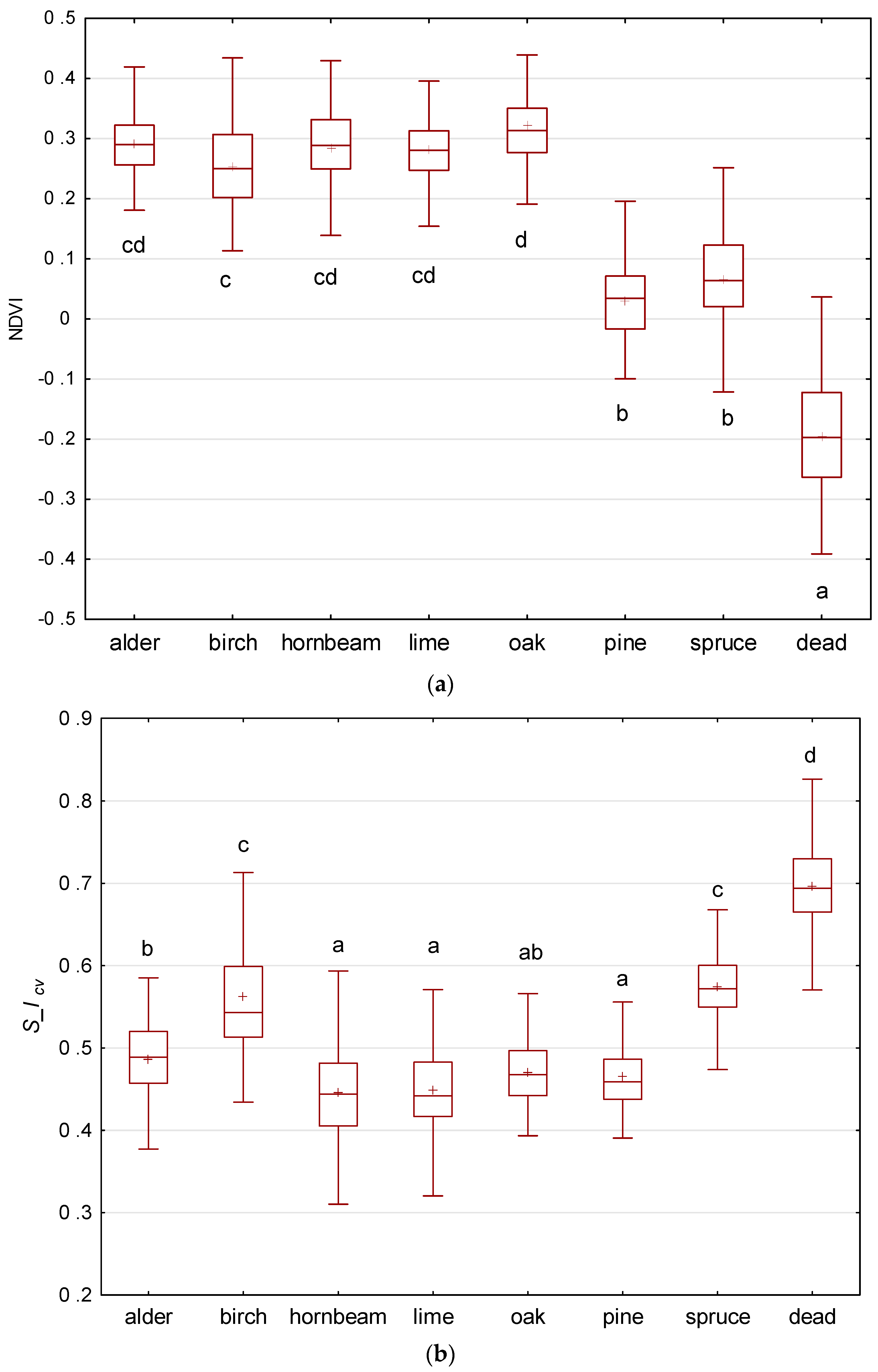
NDVI turned out to be an important predictor for distinguishing the tree health conditions and coniferous versus deciduous (Figure 6). Mean values of NDVI were positive for living trees and negative for dead trees. Additionally, NDVI values for deciduous were statistically and significantly higher than those of the coniferous classes.
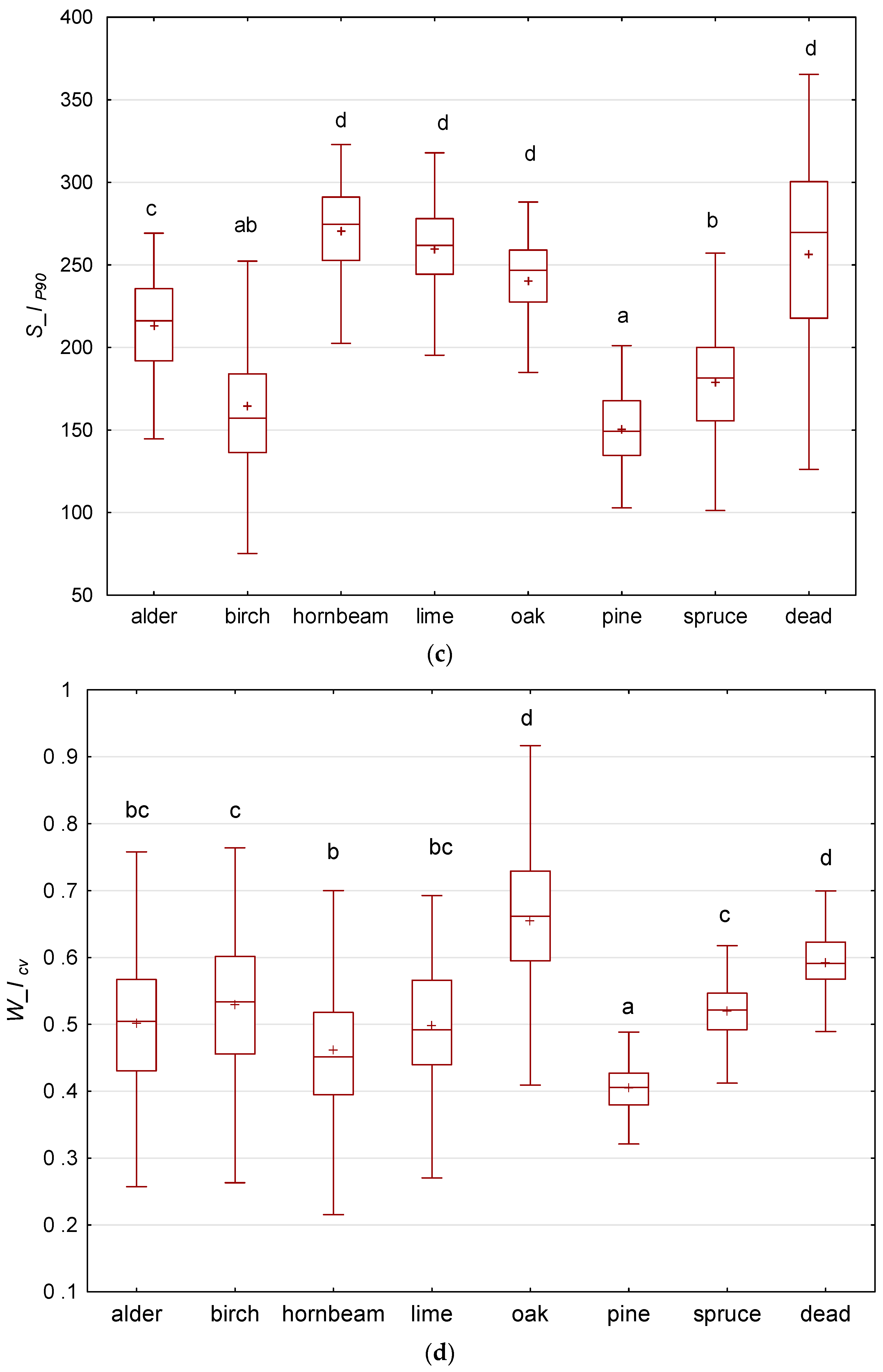
Two the most important features under the leaf-on conditions (ICV, IP90) distinguished spruce versus pine and birch versus the rest of deciduous trees (Figure 6). No significant differences between hornbeam, lime, and oak were noticed. The mean value of ICV for dead spruces was the highest one, with significant differences with other classes. IP90 in turn allowed alder to be discriminated from the other classes.
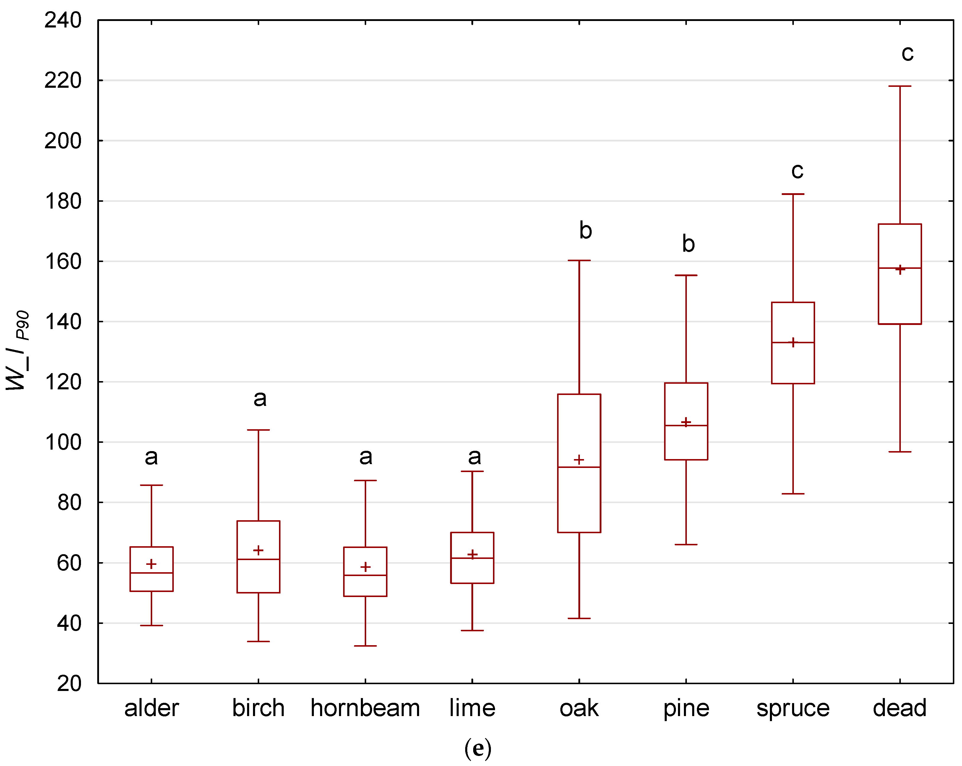
ICV under leaf-off conditions allowed pine and {dead, oak} to be separated from the other classes (Figure 6). The coefficient of variation of intensity, was the lowest for pine and the highest for dead spruces and oak. IP90 under the leaf-off conditions in turn allowed {dead and alive spruce} vs. {oak, pine} vs. {other deciduous trees} to be discriminated. Mean values of IP90 were significantly higher for coniferous trees than deciduous trees.
4. Discussion
This study evaluated and compared results to discriminate different coniferous and deciduous tree species, including dead class, in a mixed temperate forest in Poland on the basis of ALS point cloud data (leaf-on and leaf-off) and CIR imagery (leaf-on). In our research, the highest level of accuracy was obtained with the use of both point clouds and the CIR dataset, and the lowest accuracies were obtained using the ALS leaf-on dataset alone. The difference in the classification performance was minor between leaf-on and leaf-off conditions (72% ≤ OA ≤ 74% and 0.67 ≤ κ ≤ 0.70) while the classification based on both point clouds achieved satisfactory and comparable results to the classification based on combined information from all three sources (83% ≤ OA ≤ 84% and 0.81 ≤ κ ≤ 0.82). Image information (CIR variables) improved classification accuracies when comparing classification based on the leaf-on point cloud alone. The classification accuracy varied between species. The classification results for coniferous trees were always better than for deciduous trees, independent of the datasets (≥79% for both PA and UA).
In the classification based on both point clouds (leaf-on and leaf-off), the intensity features appeared to be more important than the other groups of variables, in particular the coefficient of variation, skewness, and percentiles. The NDVI was the most important CIR-based feature.
4.1. Classification Results
Several studies have discussed the influence of canopy seasonal stage on tree properties from ALS data [5,17,25,41,42,43]. Comparing both point clouds, Kim et al. [5], Kamińska et al. [25], Ørka et al. [41], and Reitberger et al. [42] reported significantly better classification results in leaf-off conditions than in leaf-on conditions (Table 7). Conversely, in Laslier et al. [43], leaf-on acquisition worked better for classification of riparian tree species. Similar to our study, Shi et al. [17] reported only a slight, but not statistically significant, improvement in classification accuracy when using leaf-off data compared to leaf-on data.
Our study revealed the necessity of temporal information (leaf-off and leaf-on variables) to classify tree species. This result is concordant with Shi et al. [17] and Kamińska et al. [25], who performed classification in a mixed forest (Table 7). Other studies provided by Kim et al. [5] and Laslier et al. [43] have also confirmed that the integration of ALS data acquired in two seasons under leaf-on and leaf-off conditions improves tree classification accuracy. Leaf-on and leaf-off conditions provide different information about the tree, and therefore are complementary. The penetration of the signal in the leaf-off season gives information about branches’ structure, while the penetration of the signal in the leaf-on season provides information about the leaf density.
It is worth pointing out that it is hard to directly compare our accuracies with other studies’ results due to differences in material that may result from many factors, e.g., species diversity, sample size, sensor type, and terrain denivelation.
4.2. Species Classification
The classification accuracy varied between species. The classification results for coniferous trees were always better than for deciduous trees independent of the datasets (≥79% for both PA and UA). Among deciduous trees, the best results were obtained for birch and alder and the lowest classification accuracies were noticed for lime, independent of the analysed datasets. Considering the combined variants, the classification accuracy was the lowest for lime and hornbeam (Table 5). These species are difficult to distinguish, as presented in Figure 6, where it can be seen that lime and hornbeam form groups with no significant differences in each of the best predictors. In general, deciduous trees were often characterised by similar intensity (e.g., Figure 6b,e) and spectral values (Figure 6a), which makes it difficult to distinguish between these species. In the conifers, significant differences were observed, especially in the coefficient of variation of intensity (Figure 6b,d), which led to a more accurate differentiation of spruce and pine. These species were also characterised by significantly lower intensity values in the leaf-on season than deciduous trees (except birch) (Figure 6c) and conversely by significantly higher values in the leaf-off season (except oak) (Figure 6e). This is in agreement with the findings of Kamińska et al. [25] and Ba et al. [18]. Kamińska et al. [25] reported high classification results for living spruce and pine, regardless of the dataset, as well as for dead spruce. According to machine learning classifiers used in the study by Ba et al. [18], the most separable trees were alders, poplars, and willows (birch was not considered), and lime trees were poorly classified.
4.3. Optimal Data Acquisition
Our study revealed the interest in using both leaf-on and leaf-off data to discriminate different coniferous and deciduous tree species in a mixed temperate forest in Poland. The leaf-off season was more favourable for conifers and oak, while hornbeam and lime obtained better results in the leaf-on season. The combination of both point clouds was favourable for birch and alder (Table 5). Our results demonstrate that differentiation between individual tree species can benefit from acquiring data in a species-appropriate period by obtaining species-specific ALS metrics. In most of the studies analysed in the temperate and boreal forests in Europe, the favourable time for acquisition was the leaf-off season [17,25,41,42], with the exception of the study by Laslier et al. [43]. This shows that the optimal conditions for obtaining data for tree species classification can depend on many factors, such as the tree species analysed, the forest type, age (which is related to the different tree structures), the climate zone, or the forest management regimes.
However, if only one ALS acquisition can be done (for economic reasons, for example), leaf-on conditions with image information included should be preferred since CIR variables significantly improved the classification accuracy when comparing classification based on the leaf-on point cloud alone for birch and conifers.
4.4. Predictor’s Importance
When we use the geometric features based on ALS, we either use more architecture-related features for data that do not contain leaves (leaf-off data), or more features related to the shape of the tree crowns for data that do contain leaves (leaf-on data). For oak, we map large branches when collecting data in the non-leafed state compared to other tree species. Different tree foliage distribution and canopy branching structures, which are often typical for the specified species, help with their recognition during species classification [28,56]. The shape of the tree crown might be advantageous for species recognition, as it is species-dependent. This has been confirmed by Ørka et al. [57], who pointed out that the major difference between spruce and birch is the rounder crown of birch and the conical shape of a spruce crown. Holmgren et al. [58] indicated that Scots pine can be separated from spruce and deciduous trees based on the tree’s relative crown base height, as they have a higher crown base than other species. However, Holmgren et al. [58] emphasized that the height of the base crown varies in the group of species and may depend on factors not included in the classification process. Axelsson et al. [35], for tree species classification, used geometric features to identify variations between species with large leaves and a dense crown and other species with thinner leaves and a sparser crown. The observed misclassifications when using only geometric features could be due to many factors, e.g., the structure of the forest and the presence of lower layers in the stands, morphological similarities between species, structural variations within the same species, external physical properties (soil, temperature), or the density of the point cloud [17].
We need to keep in mind that many geometric features are affected by tree age and tree height (which is related to age) and other properties, such as crown volume, crown shape, and the interior structure of the tree crown. The vertical structure of trees and their typical architecture can be well reflected in the ALS data when these trees grow in a sufficiently loose density without lower forest layers. When trees grow in a high compactness, there are lower forest layers in the stands and different species grow in a mixture, and thus it is difficult to maintain the typical spatial patterns of the distribution of ALS points for specific tree species after the segmentation of individual trees. This is the case in our study. The Białowieża Forest is a very complex forest, with varied structure and species composition. Since a lot of noise was captured in the ALS data due to the BF structure, the structural variables were not as important in the species-related classification.
In the classification based on both point clouds (leaf-on and leaf-off), the intensity features appeared to be more important than the other groups of variables, in particular the coefficient of variation, skewness, and percentiles. Similar results were obtained by Kamińska et al. [25], where the same intensity features indicated high-grade ratings for the discrimination of spruce, pine, and deciduous trees divided by alive or dead classes for both seasons.
Many studies have presented that the combination of ALS height information with radiometric features could achieve the complementary advantages of different details and generate better results for species classification compared to the results generated with geometric or radiometric features alone [17,29,34,59,60,61]. The backscattered signal intensity is related to the foliage type, leaf size, leaf orientation, and foliage density, providing additional possibilities for the tree species classification [5,29,30]. Image information (CIR variables) improved classification accuracies when comparing classification based on the leaf-on point cloud alone for coniferous (pine, spruce, dead) and birch. No significant improvement was noted for the rest of the deciduous trees. Image information did not improve classification accuracies under the leaf-off condition. Classification accuracy did not vary between species.
The results obtained allow us to conclude that the use of multi-temporal ALS data gives the possibility of an accurate classification of many tree species, similar to the results with the addition of information from CIR images. We assume that a denser point cloud could serve to extract more detailed structural metrics, such as the branch arrangement of a single tree, which could more reliably contribute to a more accurate tree species classification.
5. Conclusions
In this study, promising results are reported for the classification of different deciduous and coniferous tree species, including dead class, by using combined information from leaf-off and leaf-on ALS datasets and CIR aerial images. In spite of the complex stand structure and heterogeneity of the BF, the classification accuracy was fairly high.
Analysing the leaf-on and leaf-off datasets alone is not sufficient for the identification of individual tree species due to their different discriminatory power. Leaf-on and leaf-off ALS point cloud features alone produced the lowest accuracies of 72% ≤ OA ≤ 74% and 0.67 ≤ κ ≤ 0.70. It was shown that the classification based on both point clouds achieved satisfactory and comparable results to the classification based on the combined information from all three sources (83% ≤ OA ≤ 84% and 0.81 ≤ κ ≤ 0.82).
In the classification based on both point clouds (leaf-on and leaf-off), the intensity features appeared to be more important than the other groups of variables, in particular the coefficient of variation, skewness, and percentiles. The NDVI was the most important CIR-based feature.
The classification accuracy varied between species. The classification results for coniferous trees were always better than for deciduous trees, independent of the datasets. Among deciduous trees, the best results were obtained for birch and alder, and the lowest one was noticed for lime, independent of the analysed datasets.
The use of multi-temporal ALS data offers great potential in tree species classification, with the possibility of omitting optical data. Further research in this area is recommended, especially using metrics from discrete returns and full-waveform simultaneously. Studies using multi-temporal ALS data during the leaf-on season to investigate phenological changes and their impact on tree species classification are also worth considering.
Author Contributions
Conceptualization, A.K., M.L. and K.S.; methodology, A.K.; validation, A.K. and M.L.; formal analysis, A.K.; data curation, M.L.; writing—original draft preparation, A.K.; writing—review and editing, A.K, M.L. and K.S.; visualization, A.K. and M.L.; Funding: A.K. and K.S. All authors have read and agreed to the published version of the manuscript.
Funding
The analyses performed in this manuscript were funded as part of a project entitled “Comprehensive spatial analysis of the dieback of dominant tree species using multi-temporal ALS data and CIR imagery in the Białowieża Primeval Forest”, carried out in the Forest Research Institute during 2021–2023. Data was funded by the project “LIFE+ ForBioSensing PL Comprehensive monitoring of stand dynamics in Białowieża Forest supported with remote sensing techniques” which is co-funded by the EU Life Plus programme (contract number LIFE13 ENV/PL/000048) and The National Fund for Environmental Protection and Water Management in Poland (contract number 485/2014/WN10/OP-NM-LF/D).
Institutional Review Board Statement
Not applicable.
Informed Consent Statement
Not applicable.
Conflicts of Interest
The authors declare no conflict of interest.
References
- Chaurasia, A.N.; Dave, M.G.; Parmar, R.M.; Bhattacharya, B.; Marpu, P.R.; Singh, A.; Krishnayya, N.S.R. Inferring species diversity and variability over climatic gradient with spectral diversity metrics. Remote Sens. 2020, 12, 2130. [Google Scholar] [CrossRef]
- Ahmed, M.R.; Rahaman, K.R.; Hassan, Q.K. Remote sensing of wildland fire-induced risk assessment at the community level. Sensors 2018, 18, 1570. [Google Scholar] [CrossRef] [Green Version]
- Andrew, M.E.; Wulder, M.A.; Nelson, T.A. Potential contributions of remote sensing to ecosystem service assessments. Prog. Phys. Geogr. 2014, 38, 328–353. [Google Scholar] [CrossRef] [Green Version]
- Yang, D.; Fu, C.S. Mapping regional forest management units: A road-based framework in Southeastern Coastal Plain and Piedmont. For. Ecosyst. 2021, 8, 17. [Google Scholar] [CrossRef]
- Kim, S.; McGaughey, R.J.; Andersen, H.E.; Schreuder, G. Tree species differentiation using intensity data derived from leaf-on and leaf-off airborne laser scanner data. Remote Sens. Environ. 2009, 113, 1575–1586. [Google Scholar] [CrossRef]
- Brandtberg, T. Individual tree-based species classification in high spatial resolution aerial images of forests using fuzzy sets. Fuzzy Sets Syst. 2002, 132, 371–387. [Google Scholar] [CrossRef]
- Clark, M.L.; Roberts, D.A.; Clark, D.B. Hyperspectral discrimination of tropical rain forest tree species at leaf to crown scales. Remote Sens. Environ. 2005, 96, 375–398. [Google Scholar] [CrossRef]
- Immitzer, M.; Atzberger, C.; Koukal, T. Tree species classification with Random forest using very high spatial resolution 8-band worldView-2 satellite data. Remote Sens. 2012, 4, 2661–2693. [Google Scholar] [CrossRef] [Green Version]
- Hycza, T.; Stereńczak, K.; Bałazy, R. Potential use of hyperspectral data to classify forest tree species. N. Z. J. For. Sci. 2018, 48, 18. [Google Scholar] [CrossRef]
- Modzelewska, A.; Kamińska, A.; Fassnacht, F.E.; Stereńczak, K. Multitemporal hyperspectral tree species classification in the Białowieza Forest World Heritage site. For. Int. J. For. Res. 2021, 94, 464–476. [Google Scholar] [CrossRef]
- Heinzel, J.; Koch, B. Investigating multiple data sources for tree species classification in temperate forest and use for single tree delineation. Int. J. Appl. Earth Obs. Geoinf. 2012, 18, 101–110. [Google Scholar] [CrossRef]
- Ghiyamat, A.; Shafri, H.Z.M. A review on hyperspectral remote sensing for homogeneous and heterogeneous forest biodiversity assessment. Int. J. Remote Sens. 2010, 31, 1837–1856. [Google Scholar] [CrossRef]
- Deur, M.; Gašparović, M.; Balenović, I. An Evaluation of Pixel- and Object-Based Tree Species Classification in Mixed Deciduous Forests Using Pansharpened Very High Spatial Resolution Satellite Imagery. Remote Sens. 2021, 13, 1868. [Google Scholar] [CrossRef]
- Clark, M.L.; Clark, D.B.; Roberts, D.A. Small-footprint lidar estimation of sub-canopy elevation and tree height in a tropical rain forest landscape. Remote Sens. Environ. 2004, 91, 68–89. [Google Scholar] [CrossRef]
- Brandtberg, T. Classifying individual tree species under leaf-off and leaf-on conditions using airborne lidar. ISPRS J. Photogramm. Remote Sens. 2007, 61, 325–340. [Google Scholar] [CrossRef]
- Yao, W.; Krzystek, P.; Heurich, M. Tree species classification and estimation of stem volume and DBH based on single tree extraction by exploiting airborne full-waveform LiDAR data. Remote Sens. Environ. 2012, 123, 368–380. [Google Scholar] [CrossRef]
- Shi, Y.; Wang, T.; Skidmore, A.K.; Heurich, M. Important LiDAR metrics for discriminating forest tree species in Central Europe. ISPRS J. Photogramm. Remote Sens. 2018, 137, 163–174. [Google Scholar] [CrossRef]
- Ba, A.; Laslier, M.; Dufour, S.; Hubert-Moy, L. Riparian trees genera identification based on leaf-on/leaf-off airborne laser scanner data and machine learning classifiers in northern France. Int. J. Remote Sens. 2020, 41, 1645–1667. [Google Scholar] [CrossRef]
- Alonzo, M.; Bookhagen, B.; Roberts, D.A. Urban tree species mapping using hyperspectral and lidar data fusion. Remote Sens. Environ. 2014, 148, 70–83. [Google Scholar] [CrossRef]
- Dalponte, M.; Ørka, H.O.; Ene, L.T.; Gobakken, T.; Næsset, E. Tree crown delineation and tree species classification in boreal forests using hyperspectral and ALS data. Remote Sens. Environ. 2014, 140, 306–317. [Google Scholar] [CrossRef]
- Dalponte, M.; Bruzzone, L.; Gianelle, D. Tree species classification in the Southern Alps based on the fusion of very high geometrical resolution multispectral/hyperspectral images and LiDAR data. Remote Sens. Environ. 2012, 123, 258–270. [Google Scholar] [CrossRef]
- Moffiet, T.; Mengersen, K.; Witte, C.; King, R.; Denham, R. Airborne laser scanning: Exploratory data analysis indicates potential variables for classification of individual trees or forest stands according to species. ISPRS J. Photogramm. Remote Sens. 2005, 59, 289–309. [Google Scholar] [CrossRef]
- Korpela, I.; Tokola, T.; Ørka, H.O.; Koskinen, M. Small-footprint discrete-return LIDAR in tree species recognition. In Proceedings of the ISPRS Workshop on High Resolution Earth Imaging for Geospatial Information, Hannover, Germany, 2–5 June 2009. [Google Scholar]
- Hovi, A.; Korhonen, L.; Vauhkonen, J.; Korpela, I. LiDAR waveform features for tree species classification and their sensitivity to tree- and acquisition related parameters. Remote Sens. Environ. 2016, 173, 224–237. [Google Scholar] [CrossRef]
- Kamińska, A.; Lisiewicz, M.; Stereńczak, K.; Kraszewski, B.; Sadkowski, R. Species-related single dead tree detection using multi-temporal ALS data and CIR imagery. Remote Sens. Environ. 2018, 219, 31–43. [Google Scholar] [CrossRef]
- Koenig, K.; Höfle, B. Full-Waveform Airborne Laser Scanning in Vegetation Studies—A Review of Point Cloud and Waveform Features for Tree Species Classification. Forests 2016, 7, 198. [Google Scholar] [CrossRef] [Green Version]
- Harikumar, A.; Paris, C.; Bovolo, F.; Bruzzone, L. A Crown Quantization-Based Approach to Tree-Species Classification Using High-Density Airborne Laser Scanning Data. IEEE Trans. Geosci. Remote Sens. 2020, 59, 4444–4453. [Google Scholar] [CrossRef]
- Holmgren, J.; Persson, Å. Identifying species of individual trees using airborne laser scanner. Remote Sens. Environ. 2004, 90, 415–423. [Google Scholar] [CrossRef]
- Suratno, A.; Seielstad, C.; Queen, L. Tree species identification in mixed coniferous forest using airborne laser scanning. ISPRS J. Photogramm. Remote Sens. 2009, 64, 683–693. [Google Scholar] [CrossRef]
- Korpela, I.; Ørka, H.; Maltamo, M.; Tokola, T.; Hyyppä, J. Tree Species Classification Using Airborne LiDAR—Effects of Stand and Tree Parameters, Downsizing of Training Set, Intensity Normalization, and Sensor Type. Silva Fenn. 2010, 44, 319–339. [Google Scholar] [CrossRef] [Green Version]
- Baltsavias, E.P. Airborne laser scanning: Basic relations and formulas. ISPRS J. Photogramm. Remote Sens. 1999, 54, 199–214. [Google Scholar] [CrossRef]
- Korpela, I.; Ørka, H.O.; Hyyppä, J.; Heikkinen, V.; Tokola, T. Range and AGC normalization in airborne discrete-return LiDAR intensity data for forest canopies. ISPRS J. Photogramm. Remote Sens. 2010, 65, 369–379. [Google Scholar] [CrossRef]
- Ørka, H.O.; Gobakken, T.; Næsset, E.; Ene, L.; Lien, V. Simultaneously acquired airborne laser scanning and multispectral imagery for individual tree species identification. Can. J. Remote Sens. 2012, 38, 125–138. [Google Scholar] [CrossRef]
- Yu, X.; Hyyppä, J.; Litkey, P.; Kaartinen, H.; Vastaranta, M.; Holopainen, M. Single-sensor solution to tree species classification using multispectral airborne laser scanning. Remote Sens. 2017, 9, 108. [Google Scholar] [CrossRef] [Green Version]
- Axelsson, A.; Lindberg, E.; Olsson, H. Exploring Multispectral ALS Data for Tree Species Classification. Remote Sens. 2018, 10, 183. [Google Scholar] [CrossRef] [Green Version]
- Budei, B.C.; St-onge, B.; Hopkinson, C.; Audet, F. Identifying the genus or species of individual trees using a three-wavelength airborne lidar system. Remote Sens. Environ. 2018, 204, 632–647. [Google Scholar] [CrossRef]
- Amiri, N.; Krzystek, P.; Heurich, M.; Skidmore, A. Classification of Tree Species as Well as Standing Dead Trees Using Triple Wavelength ALS in a Temperate Forest. Remote Sens. 2019, 11, 2614. [Google Scholar] [CrossRef] [Green Version]
- Heinzel, J.; Koch, B. Exploring full-waveform LiDAR parameters for tree species classification. Int. J. Appl. Earth Obs. Geoinf. 2011, 13, 152–160. [Google Scholar] [CrossRef]
- Liang, X.; Hyyppä, J.; Matikainen, L. Deciduous-Coniferous Tree Classification Using Difference Between First and Last Pulse Laser Signatures. In Proceedings of the ISPRS Workshop on Laser Scanning 2007 and SilviLaser 2007, Espoo, Finland, 12–14 September 2007; pp. 253–257. [Google Scholar]
- Hollaus, M.; Mücke, W.; Höfle, B.; Dorigo, W.; Pfeifer, N.; Wagner, W.; Bauerhansl, C.; Regner, B. Tree species classification based on full-waveform airborne laser scanning data. In Proceedings of the Silvilaser, College Station, TX, USA, 14–16 October 2009; pp. 54–62. [Google Scholar]
- Ørka, H.O.; Næsset, E.; Bollandsås, O.M. Effects of different sensors and leaf-on and leaf-off canopy conditions on echo distributions and individual tree properties derived from airborne laser scanning. Remote Sens. Environ. 2010, 114, 1445–1461. [Google Scholar] [CrossRef]
- Reitberger, J.; Krzystek, P.; Stilla, U. Analysis of full waveform LIDAR data for the classification of deciduous and coniferous trees. Int. J. Remote Sens. 2008, 29, 1407–1431. [Google Scholar] [CrossRef]
- Laslier, M.; Ba, A.; Hubert-Moy, L.; Dufour, S. Comparison of leaf-on and leaf-off ALS data for mapping riparian tree species. In Proceedings of the SPIE 2017, Warsaw, Poland, 12–15 September 2017. [Google Scholar]
- Yu, X.; Litkey, P.; Hyyppä, J.; Holopainen, M.; Vastaranta, M. Assessment of low density full-waveform airborne laser scanning for individual tree detection and tree species classification. Forests 2014, 5, 1011–1031. [Google Scholar] [CrossRef] [Green Version]
- Sumnall, M.; Hill, R.; Hinsley, S. Comparison of small-footprint discrete return and full waveform airborne lidar data for estimating multiple forest variables. Remote Sens. Environ. 2016, 173, 214–223. [Google Scholar] [CrossRef] [Green Version]
- Stereńczak, K.; Kraszewski, B.; Mielcarek, M.; Kamińska, A.; Lisiewicz, M.; Modzelewska, A.; Sadkowski, R.; Białczak, M.; Piasecka, Ż.; Wilkowska, R. The Białowieża Forest monitoring with the use of remote sensing data. In Zimowa Szkoła Leśna XI Sesja—Zastosowanie Geoinformatyki w Leśnictwie; Instytut Badawczy Leśnictwa: Sękocin Stary, Poland, 2020; pp. 99–107. (In Polish) [Google Scholar]
- Erfanifard, Y.; Stereńczak, K.; Kraszewski, B.; Kamińska, A. Development of a robust canopy height model derived from ALS point clouds for predicting individual crown attributes at the species level. Int. J. Remote Sens. 2018, 39, 9206–9227. [Google Scholar] [CrossRef]
- Stereńczak, K.; Kraszewski, B.; Mielcarek, M.; Piasecka, Ż.; Lisiewicz, M.; Heurich, M. Mapping individual trees with airborne laser scanning data in an European lowland forest using a self-calibration algorithm. Int. J. Appl. Earth Obs. Geoinf. 2020, 93, 102191. [Google Scholar] [CrossRef]
- Breiman, L. Random Forests. Mach. Learn. 2001, 45, 5–32. [Google Scholar] [CrossRef] [Green Version]
- R Core Team. R: A Language and Environment for Statistical Computing; R Foundation for Statistical Computing: Vienna, Austria, 2020. [Google Scholar]
- Breiman, L.; Friedman, J.H.; Olshen, R.A.; Stone, C.J. Classification and Regression Trees, 1st ed.; Routledge: Boca Raton, FL, USA, 1984. [Google Scholar]
- Liaw, A.; Wiener, M. Classification and Regression by randomForest. R News 2002, 3, 18–22. [Google Scholar]
- Cohen, J. A Coefficient of Agreement for Nominal Scales. Educ. Psychol. Meas. 1960, 20, 37–46. [Google Scholar] [CrossRef]
- Story, M.; Congalton, R.G. Accuracy Assessment: A User’s Perspective. Photogramm. Eng. Remote Sens. 1986, 52, 397–399. [Google Scholar]
- Bradley, J. Distribution-Free Statistical Tests; Prentice-Hall: Hoboken, NJ, USA, 1968. [Google Scholar]
- Ørka, H.O.; Næsset, E.; Bollandsås, O.M. Utilizing airborne laser intensity for tree species classification. In Proceedings of the ISPRS Workshop on Laser Scanning 2007 and SilviLaser 2007, Espoo, Finland, 12–14 September 2007; pp. 300–304. [Google Scholar]
- Ørka, H.O.; Næsset, E.; Bollandsås, O.M. Classifying species of individual trees by intensity and structure features derived from airborne laser scanner data. Remote Sens. Environ. 2009, 113, 1163–1174. [Google Scholar] [CrossRef]
- Holmgren, J.; Persson, Å.; Söderman, U. Species identification of individual trees by combining high resolution LiDAR data with multi-spectral images. Int. J. Remote Sens. 2008, 29, 1537–1552. [Google Scholar] [CrossRef]
- Zhang, Z.; Liu, X. Support vector machines for tree species identification using LiDAR-derived structure and intensity variables. Geocarto Int. 2013, 28, 364–378. [Google Scholar] [CrossRef]
- Lin, Y.; Hyyppä, J. A comprehensive but efficient framework of proposing and validating feature parameters from airborne LiDAR data for tree species classification. Int. J. Appl. Earth Obs. Geoinf. 2016, 46, 45–55. [Google Scholar] [CrossRef]
- You, H.T.; Lei, P.; Li, M.S.; Ruan, F.Q. Forest pecies classification based on three-dimensional coordinate and intensity information of airborne LiDAR data with Random Forest method. In Proceedings of the International Archives of the Photogrammetry, Remote Sensing and Spatial Information Sciences, Guilin, China, 15–17 November 2019; XLII-3/W10, pp. 117–123. [Google Scholar]
Figure 1.
Polish part of the Białowieża Forest. In addition, data samples for one monitoring plot are presented. From top to bottom: a rasterised point cloud with RGB values, canopy height model, and point cloud density. The polygons represent the results of individual tree detection, while the points represent the locations of the trees measured in the field.

Figure 2.
Presentation of examples of selected trees showing a properly segmented tree and its profile on the leaf-on (left) and leaf-off (right) point cloud.
Figure 2.
Presentation of examples of selected trees showing a properly segmented tree and its profile on the leaf-on (left) and leaf-off (right) point cloud.

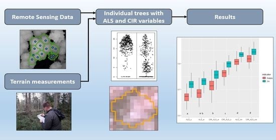
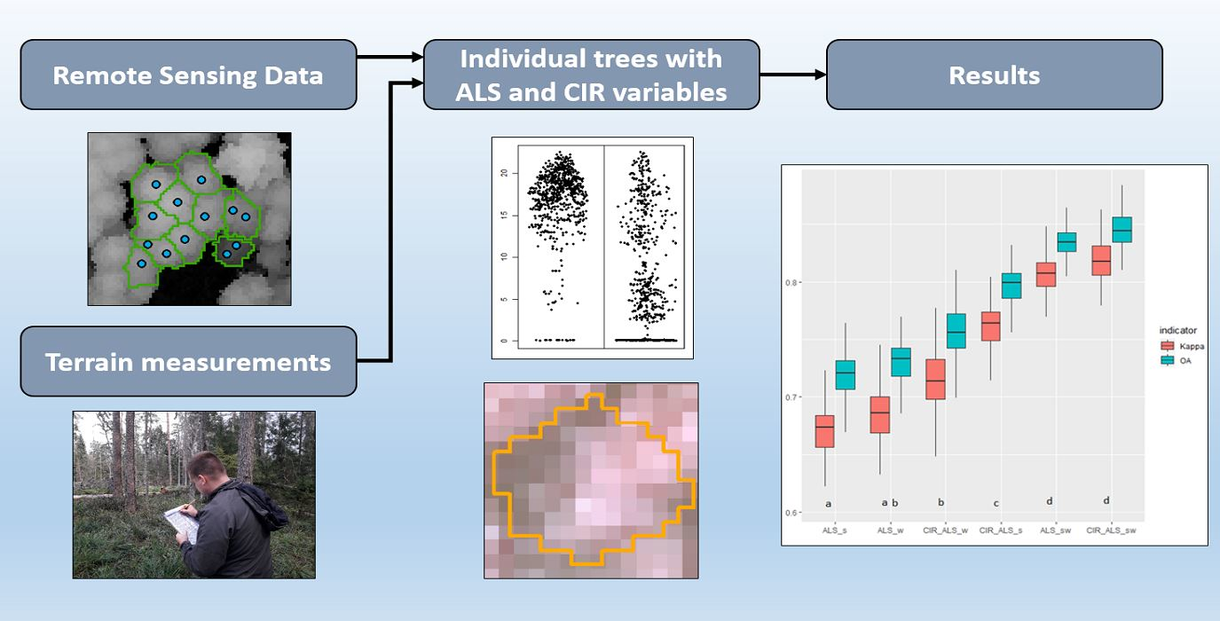
Figure 3.
Methodological framework developed in this study.

Figure 4.
Box-and-whisker plots of accuracies for different classification variants based on both point clouds and CIR. The first and third quartiles define the box, the median is shown as “—”, and the whisker defines the range of the data without outliers. Letters ‘a, b, c, d’ identify homogenous groups with no significant differences (based on McNemar’s test). The ALS is the point cloud from the leaf-on (S) or/and leaf-off (W) season, whereas the CIR is the spectral information derived from the colour-infrared images.

Figure 5.
Box-and-whisker plot of the producer’s (PA) and user’s (UA) accuracies of specific tree species for the classification based on both point clouds and image information. The first and third quartiles define the box, the median is shown as “—”, and the whisker defines the range of the data without outliers. The ALS is the point cloud from the leaf-on (S) or/and leaf-off (W) season, whereas the CIR is the spectral information derived from the colour-infrared images.

Figure 6.
Box-and-whisker plot of the best predictors: (a) NDVI, (b) S_ICV, (c) S_IP90, (d) W_ICV, and (e) W_IP90 for the sample trees analysed in the study. The first and third quartiles define the box, the median is shown as “—”, the mean is shown as “+”, and the whisker defines the range of the data without outliers. Letters a, b, … above the boxes identify groups with no significant differences (based on the Kruskal–Wallis test). The ALS is the point cloud from the leaf-on (S) or/and leaf-off (W) season, whereas the CIR is the spectral information derived from the colour-infrared images. The descriptions of the predictors are included in Table 3 and Table 4.


Table 1.
Studies comparing ALS data from leaf-off and leaf-on seasons.
| Author | Classes | Species | Study Area |
|---|---|---|---|
| Ba et al. [18] | 8 | oak, alder, poplar, ash, lime, chestnut, willow, beech | Normandy, France |
| Laslier et al. [43] | 8 | ||
| Kim et al. [5] | 2 | Broadleaves (birch, bigleaf maple, elm, magnolia, malus, oak, sorbus, prunus), coniferous (cedar, Douglas fir, larch, pinus, redwood, spruce, western hemlock) | Washington Park Arboretum, Seattle, Washington, USA |
| Shi et al. [17] | 6 | Spruce, beech, fir, birch, maple, rowan | Bavarian Forest National Park, Germany |
| Reitberger et al. [42] | 2 | Coniferous (spruce), deciduous (beech, maple) | |
| Kamińska et al. [25] | 6 | Deciduous (alder, ash, aspen, birch, elm, hornbeam, lime, maple, oak), pine, spruce—divided by dead and alive | Białowieża Forest, Poland |
| Ørka et al. [41] | 2 | Spruce, deciduous (birch, aspen) | Østmarka nature reserve, Norway |
Table 2.
Number (n) of selected reference trees divided into particular species. Additionally, information about the minimum (Min), maximum (Max), and mean (with standard deviation (SD)) height of trees in each class is presented.
Table 2.
Number (n) of selected reference trees divided into particular species. Additionally, information about the minimum (Min), maximum (Max), and mean (with standard deviation (SD)) height of trees in each class is presented.
| Species | n | Min (m) | Max (m) | Mean (SD) (m) |
|---|---|---|---|---|
| birch | 117 | 14.4 | 32.8 | 23.5 (4.9) |
| oak | 125 | 13.9 | 36.4 | 28.1 (5.2) |
| hornbeam | 117 | 7.9 | 31.0 | 21.7 (4.5) |
| lime | 98 | 15.4 | 31.8 | 23.6 (4.0) |
| alder | 222 | 10.1 | 33.6 | 25.3 (4.2) |
| pine | 198 | 15.4 | 39.6 | 27.2 (5.2) |
| spruce | 240 | 16.5 | 40.5 | 27.7 (4.9) |
| dead | 113 | 18.4 | 41.4 | 30.5 (5.4) |
Table 3.
Tree features derived from ALS data and spectral information.
| Feature | Description |
|---|---|
| Structural features | |
| Hmean | Arithmetic mean of all normalized heights from the point cloud |
| Hsd | The standard deviation of all normalized heights from the point cloud |
| HCV | The coefficient of variation of all normalized heights from the point cloud |
| Hskew | Skewness of all normalized heights from the point cloud |
| Hkurt | Kurtosis of normalized heights from the point cloud |
| Haad_mean | Average absolute deviation of all normalized heights from the point cloud: mean(abs(X-mean(X)) |
| Haad_median | Median absolute deviation of all normalized heights from the point cloud: median(abs(X-mean(X)) |
| HP10–HP90 | 10th to 90th percentiles of all normalized heights from the point cloud |
| HIQ | Inter-percentile range of all normalized heights from the point cloud: HP75–HP25 |
| Pmean | The ratio of the total number of points above the mean to the total number of all points |
| Pmedian | The ratio of the total number of points above the median to the total number of all points |
| CanRR | Canopy relief ratio of points: (avg(X)-min(X))/(max(X)-min(X)) |
| Additional features | |
| Pfe_all | The proportion of first returns |
| Psingle_all | The proportion of single returns |
| Intensity features | |
| Imean | Mean of intensity values |
| Isd | The standard deviation of intensity values |
| ICV | The coefficient of variation of intensity values |
| Iskew | Skewness of intensity values |
| Ikurt | Kurtosis of intensity values |
| Iaad_mean | Average absolute deviation of intensity values |
| Iaad_median | Median absolute deviation of intensity values |
| IP10–IP90 | 10th to 90th percentiles of intensity values |
| IIQ | Inter-percentile range of intensity values |
| CIR features | |
| NDVI | Normalized differenced vegetation index |
| NIRmean | Mean value of reflectance in the near-infrared band |
| NIRmedian | Median value of reflectance in the near-infrared band |
| NIRsd | The standard deviation of reflectance in the near-infrared band |
| Rmean | Mean value of reflectance in the red band |
| Rmedian | Median value of reflectance in the red band |
| Rsd | The standard deviation of reflectance in the red band |
| Gmean | Mean value of reflectance in the green band |
| Gmedian | Median value of reflectance in the green band |
| Gsd | The standard deviation of reflectance in the green band |
Table 4.
Description of symbol designations of particular variants.
| Symbol | Description |
|---|---|
| ALS | Variant with the usage of ALS point cloud |
| CIR | Variant with the usage of CIR aerial images |
| S | Point cloud from the leaf-on season (summer) |
| W | Point cloud from the leaf-off season (winter) |
Table 5.
F1-scores of the classification results for different sets of features. Letters “a, b, c” identify groups with no significant differences (based on McNemar’s tests). The ALS is the point cloud from the leaf-on (S) or/and leaf-off (W) season, whereas the CIR is the spectral information derived from the colour-infrared images.
| Birch | Alder | Oak | Hornbeam | Lime | Pine | Spruce | Dead | |
|---|---|---|---|---|---|---|---|---|
| ALSS | 0.51(a) | 0.69(a) | 0.58(a) | 0.67(b) | 0.51(b) | 0.84(a) | 0.83(a) | 0.88(a) |
| CIR_ALSS | 0.80(b) | 0.74(ab) | 0.59(ab) | 0.68(b) | 0.53(b) | 0.93(b) | 0.92(b) | 0.98(b) |
| ALSW | 0.53(a) | 0.67(a) | 0.68(bc) | 0.39(a) | 0.34(a) | 0.95(b) | 0.94(b) | 0.94(b) |
| CIR_ALSW | 0.58(a) | 0.69(ab) | 0.76(c) | 0.40(a) | 0.37(ab) | 0.95(b) | 0.95(b) | 0.98(b) |
| ALSSW | 0.86(c) | 0.78(b) | 0.72(c) | 0.66(b) | 0.53(b) | 0.96(b) | 0.95(b) | 0.96(b) |
| CIR_ALSSW | 0.87(c) | 0.78(b) | 0.75(c) | 0.68(b) | 0.55(b) | 0.96(b) | 0.96(b) | 0.98(b) |
Table 6.
The most important predictors in the classification variants. The ALS is the point cloud from the leaf-on (S) or/and leaf-off (W) season, whereas the CIR is the spectral information derived from the colour-infrared images. The descriptions of the predictors and variants are included in Table 3 and Table 4, respectively.
| Variants | Predictors |
|---|---|
| ALSS | S_ICV, S_IP90, S_IIQR, S_IP50, S_Iskew |
| ALSW | W_ICV, W_Psingle_all, W_IP40, W_Iskew, W_Pfe_all |
| ALSSW | W_Iskew, W_IP40, W_IP90, W_Psingle_all, S_ICV, W_ICV, S_Iskew, S_IP90 |
| CIR_ALSS | NDVI, S_ICV, Rmean, S_IP90, S_IIQR, S_IP50, S_Iskew |
| CIR_ALSW | W_ICV, W_Psingle_all, W_IP40, NDVI, W_Iskew, W_Pfe_all |
| CIR_ALSSW | W_Iskew, NDVI, S_ICV, W_IP40, W_IP90, W_Psingle_all, W_ICV, S_Iskew, S_IP90 |
Table 7.
Species classification accuracies for studies comparing or integrating ALS data from both seasons.
Table 7.
Species classification accuracies for studies comparing or integrating ALS data from both seasons.
| Author | Accuracy | |||
|---|---|---|---|---|
| Classes (n) | Leaf-On | Leaf-Off | Leaf-On and Leaf-Off | |
| Laslier et al. [43] | 8 | OA = 48.1% κ = 0.40 | OA = 45.9% κ = 0.37 | OA = 52.5% κ = 0.45 |
| Kim et al. [5] | 2 | OA = 73.1% | OA = 83.4%, | OA = 90.6% |
| Shi et al. [17] | 6 | OA = 58% κ = 0.47 | OA = 62% κ = 0.51 | OA = 66.5% κ = 0.58 |
| Reitberger et al. [42] | 2 | OA = 85.4% | OA = 95.7% | |
| Kamińska et al. [25] | 6 | OA = 81.4% κ = 0.76 | OA = 87.6% κ = 0.84 | OA = 93.2% κ = 0.91 |
| Ørka et al. [41] | 2 | OA = 0.87 κ = 0.74 | OA = 0.97 κ = 0.94 | |
Publisher’s Note: MDPI stays neutral with regard to jurisdictional claims in published maps and institutional affiliations. |
© 2021 by the authors. Licensee MDPI, Basel, Switzerland. This article is an open access article distributed under the terms and conditions of the Creative Commons Attribution (CC BY) license (https://creativecommons.org/licenses/by/4.0/).
Share and Cite
MDPI and ACS Style
Kamińska, A.; Lisiewicz, M.; Stereńczak, K. Single Tree Classification Using Multi-Temporal ALS Data and CIR Imagery in Mixed Old-Growth Forest in Poland. Remote Sens. 2021, 13, 5101. https://0-doi-org.brum.beds.ac.uk/10.3390/rs13245101
AMA Style
Kamińska A, Lisiewicz M, Stereńczak K. Single Tree Classification Using Multi-Temporal ALS Data and CIR Imagery in Mixed Old-Growth Forest in Poland. Remote Sensing. 2021; 13(24):5101. https://0-doi-org.brum.beds.ac.uk/10.3390/rs13245101
Chicago/Turabian StyleKamińska, Agnieszka, Maciej Lisiewicz, and Krzysztof Stereńczak. 2021. "Single Tree Classification Using Multi-Temporal ALS Data and CIR Imagery in Mixed Old-Growth Forest in Poland" Remote Sensing 13, no. 24: 5101. https://0-doi-org.brum.beds.ac.uk/10.3390/rs13245101
Note that from the first issue of 2016, this journal uses article numbers instead of page numbers. See further details here.