
Improving Heterogeneous Forest Height Maps by Integrating GEDI-Based Forest Height Information in a Multi-Sensor Mapping Process

 , , ,
, , ,
Abstract
:
1. Introduction
2. Materials and Methods
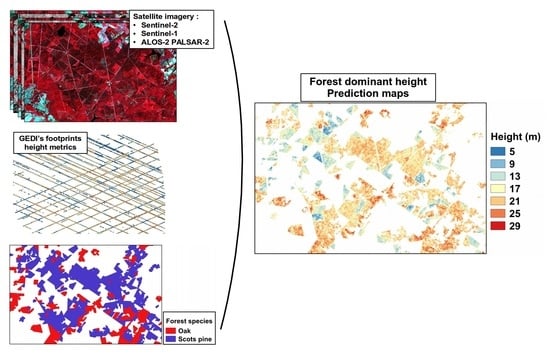
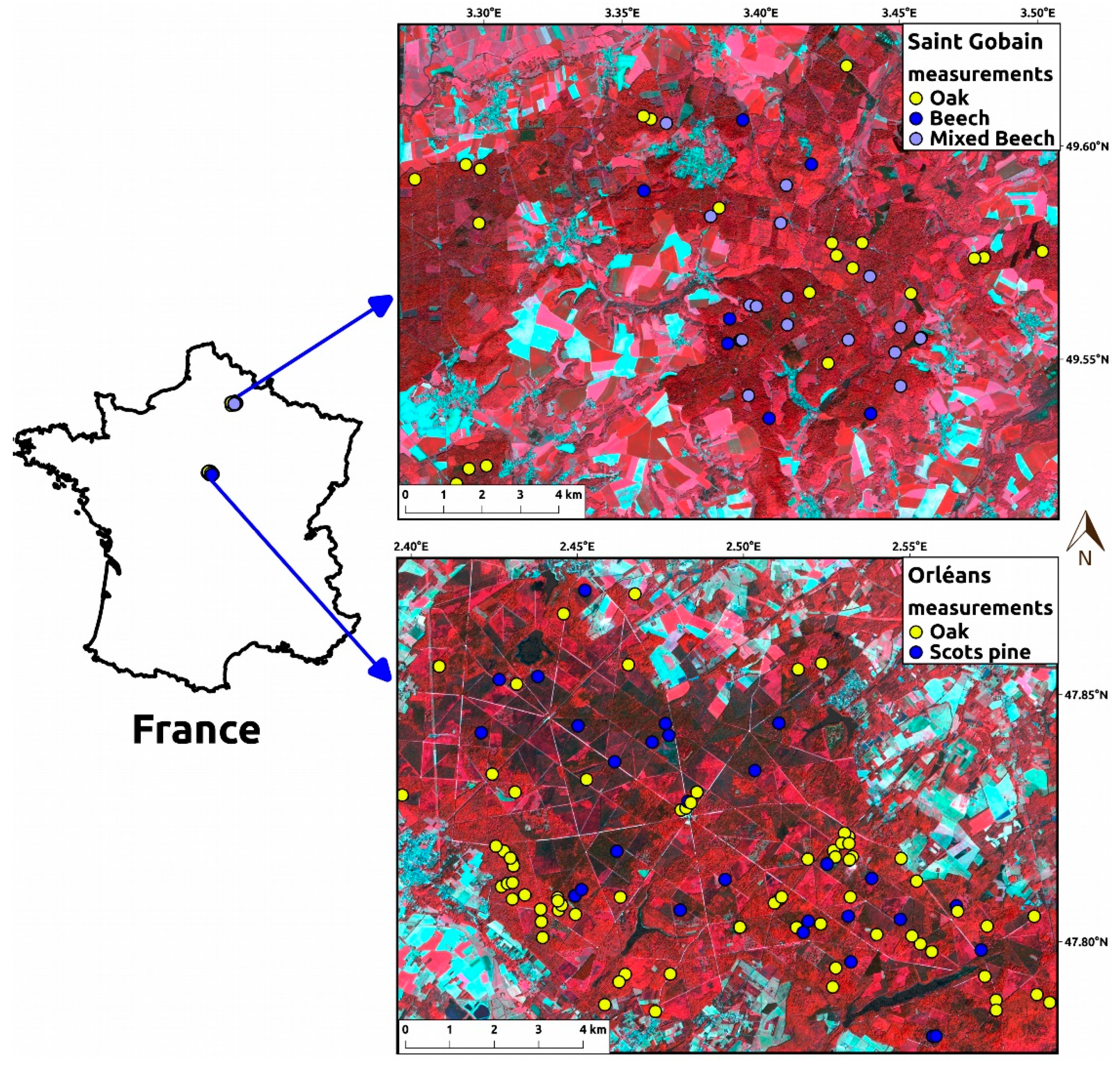
2.1. Study Sites and In Situ Data
2.2. Remote Sensing Data
2.2.1. Satellite Imagery
2.2.2. GEDI Data
2.3. Methodology
2.3.1. Processing of Ancillary Products
2.3.2. Estimation of Forest Parameters
- ONF Hdom measurements or GEDI RH95% are used as reference data, and the remote sensing features from Section 2.3 are used as predictive variables.
- Reference data and remote sensing features are fed to a Support Vector Machine (SVR) algorithm for regression; the SVR has 3 key parameters that need to be optimised: cost parameter, gamma and epsilon.
- Validation is made with a leave-one-out (LOO) cross-validation method when using the ONF measurement data because the number of samples is very low for these data (21 to 75 samples); when the reference data is GEDI RH95, we use a stratified K-fold cross-validation method.
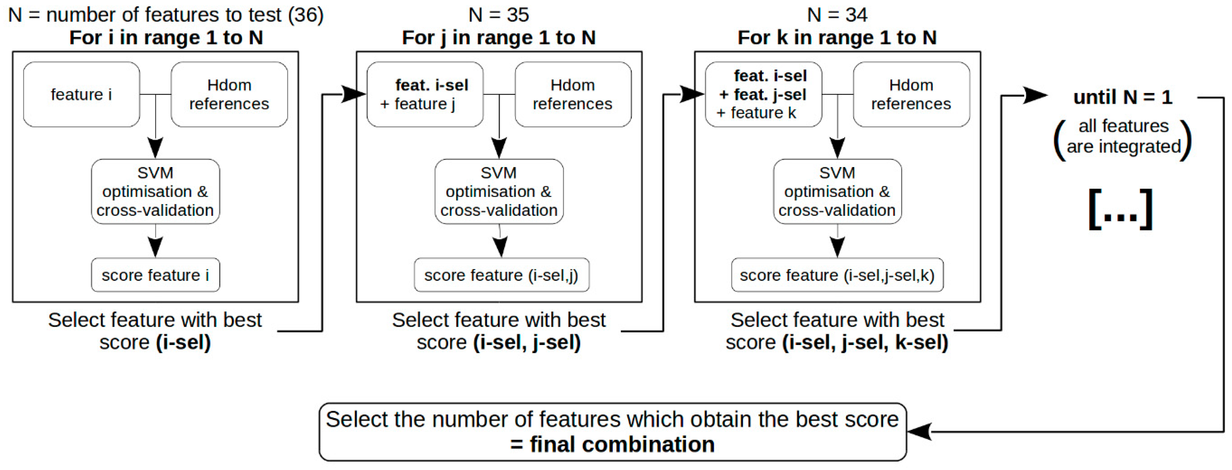
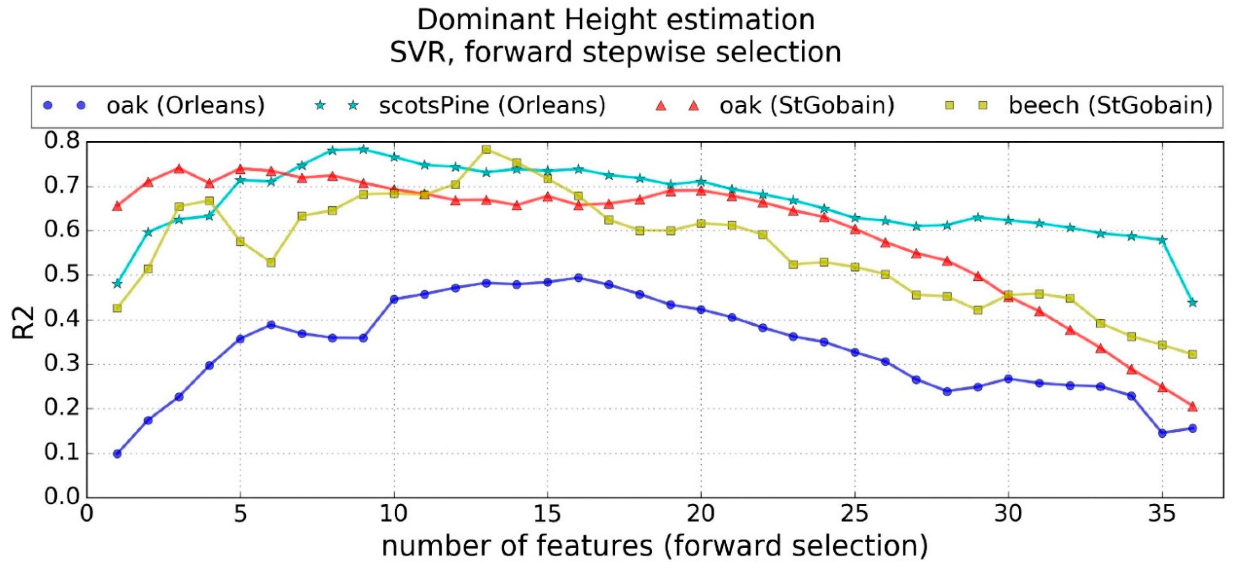
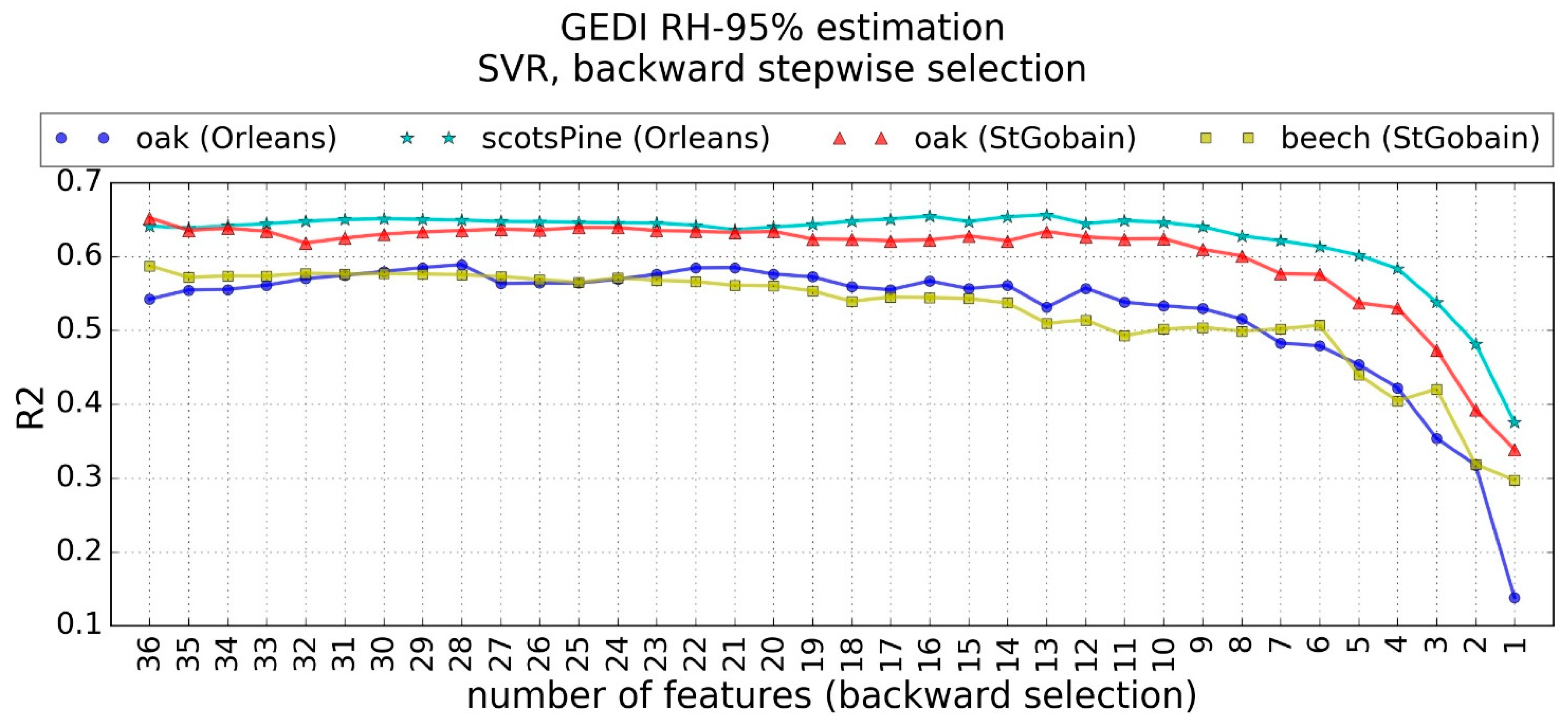
- We used a stepwise approach for feature selection. It is an iterative process that starts with 1 feature or N features and iteratively adds or removes features, respectively, for forward and backward selection. Within the 1 to N feature combinations, the one with the lowest RMSE is considered the best predictive set we can obtain on the dataset.
3. Results
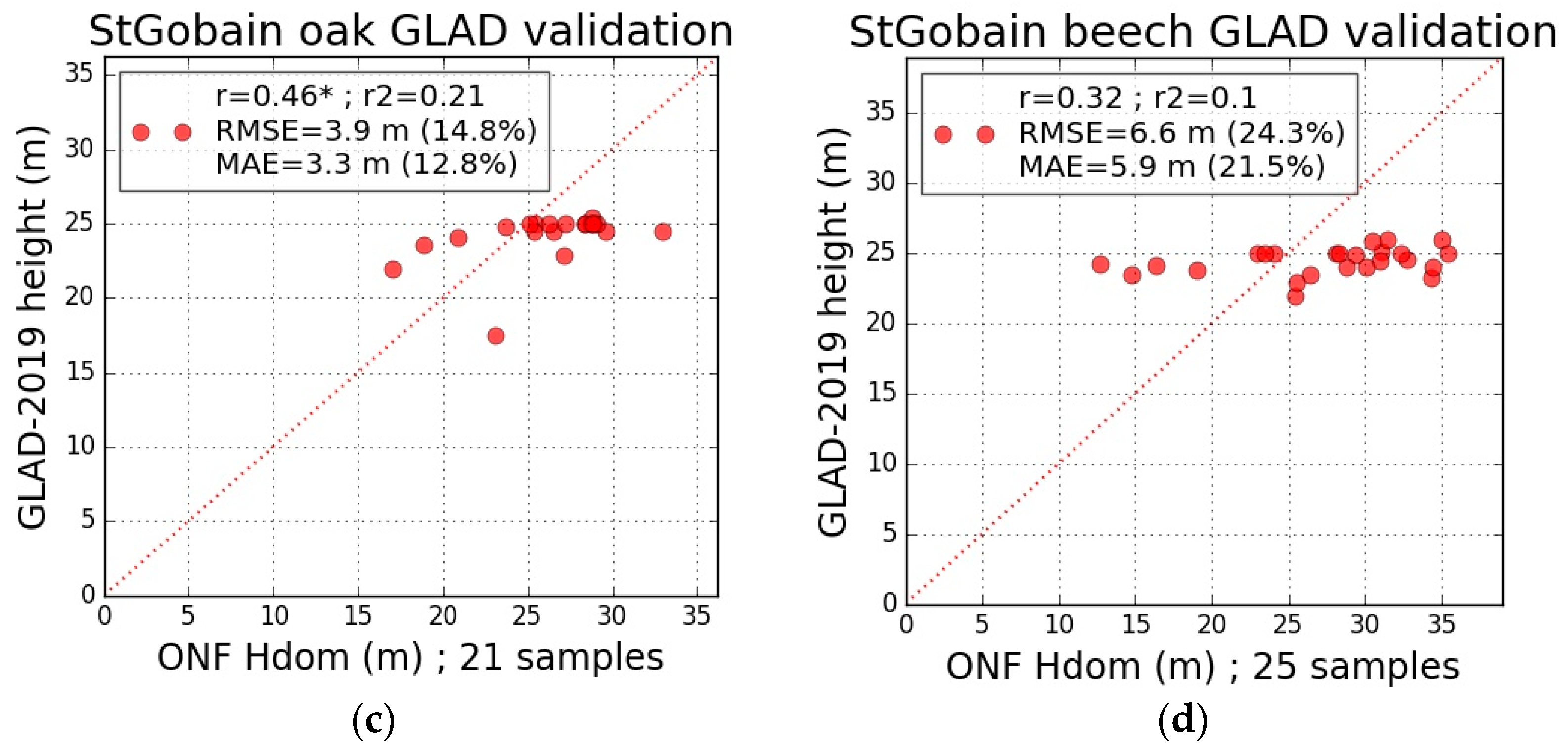
3.1. GLAD-2019 Canopy Height Map Evaluation
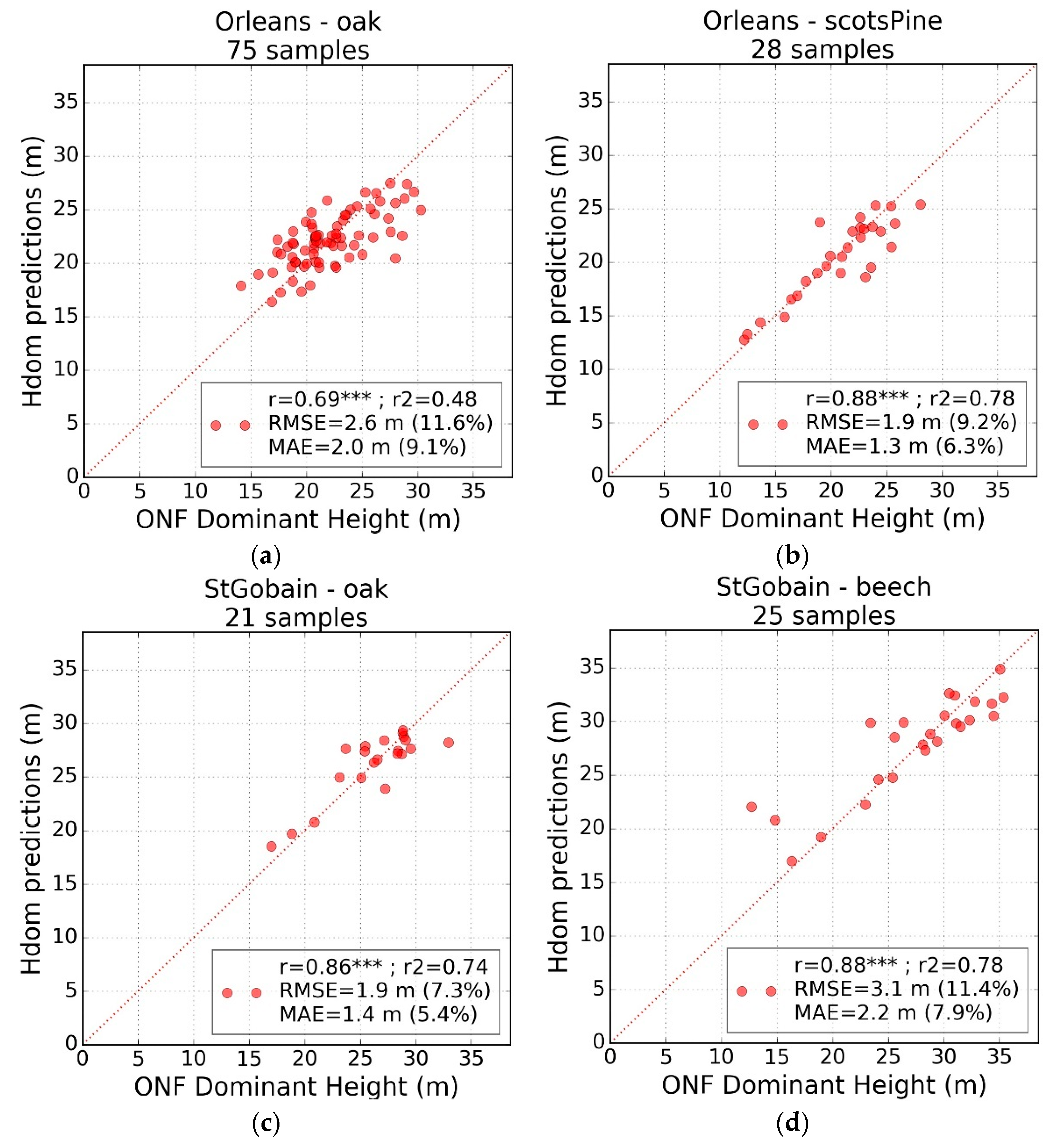
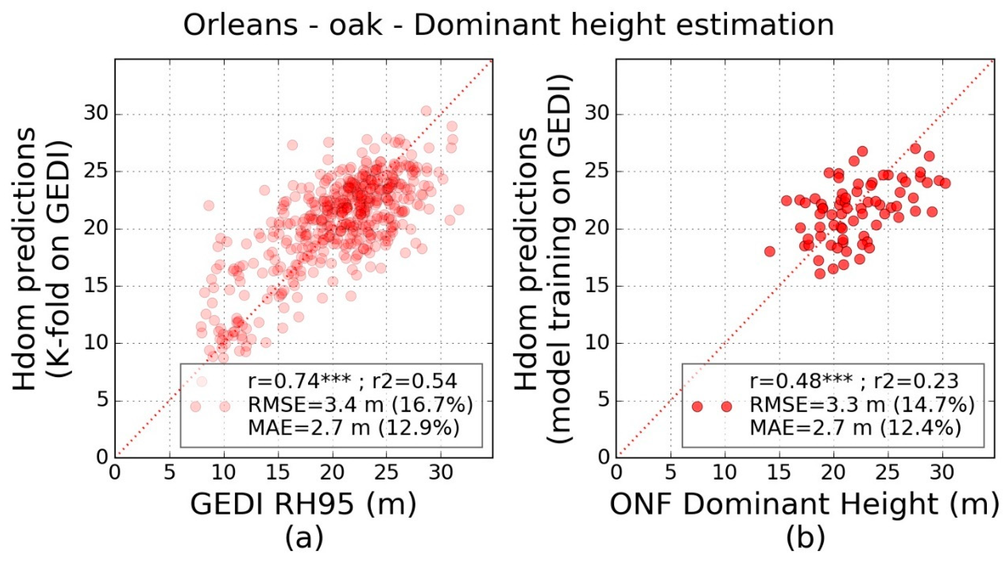
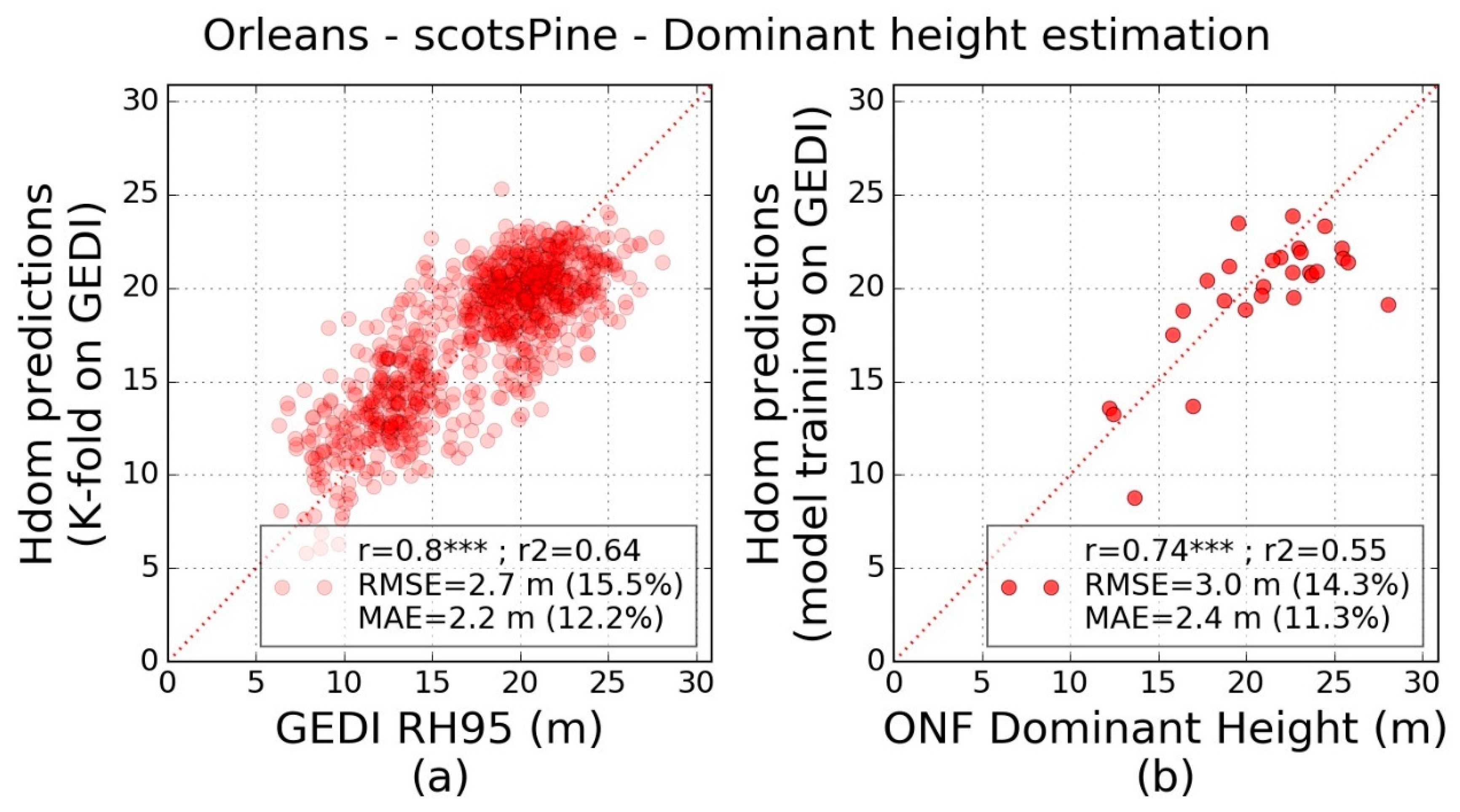
3.2. Dominant Height Estimation Using Field Campaign as Reference Data
3.3. Dominant Height Estimation Using GEDI Height Metrics as Reference Data
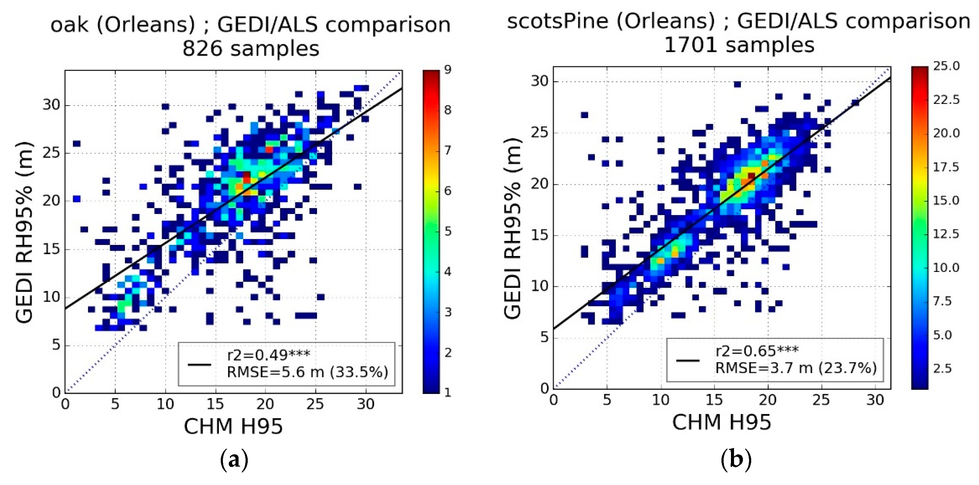
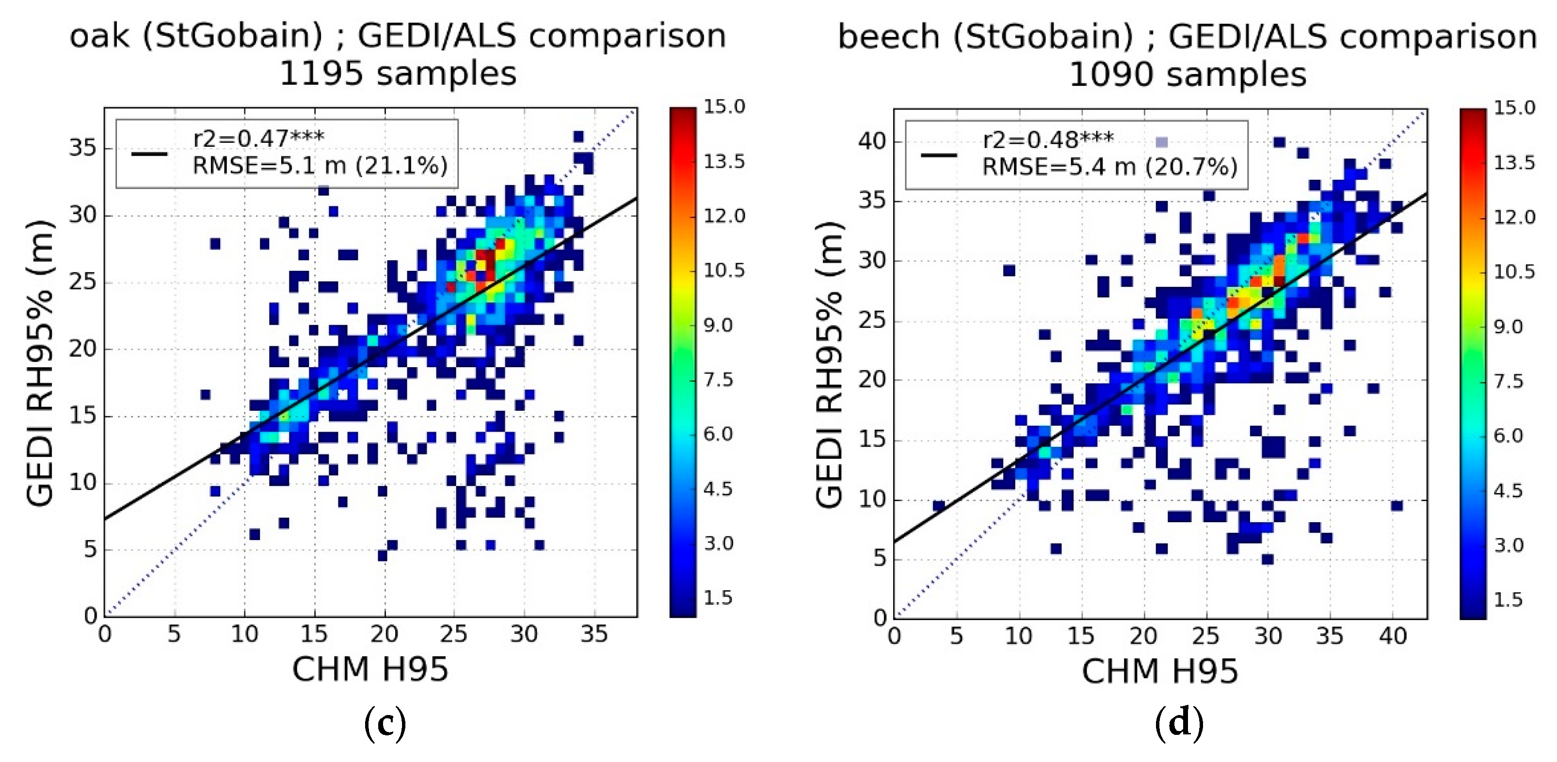
3.3.1. GEDI RH95% Comparison with ALS Data
3.3.2. Using GEDI RH95% Instead of Field Data
4. Discussion
5. Conclusions
Author Contributions
Funding
Data Availability Statement
Acknowledgments
Conflicts of Interest
Appendix A


| Orléans | StGobain | ||||
|---|---|---|---|---|---|
| Oak | Scots Pine | Oak | Beech | ||
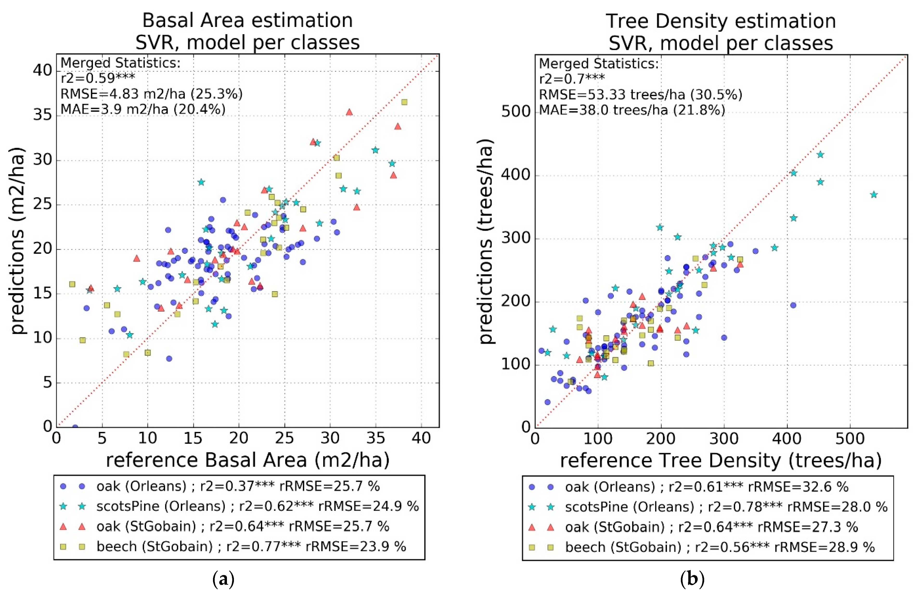
| BA (m2/ha) | r2 | 0.37 | 0.62 | 0.64 | 0.77 |
| RMSE | 4.62 (25.7%) | 5.18 (24.9%) | 5.38 (25.7%) | 4.57 (23.9%) | |
| MAE | 3.94 (22.0%) | 4.17 (20.1%) | 4.29 (20.4%) | 3.14 (16.5%) | |
| Density (tree/ha) | r2 | 0.61 | 0.78 | 0.64 | 0.56 |
| RMSE | 53.4 (32.6%) | 66.2 (28.0%) | 42.3 (27.3%) | 44.3 (28.9%) | |
| MAE | 36.5 (22.3%) | 47.3 (20.0%) | 35.5 (22.9%) | 34.2 (22.3%) | |
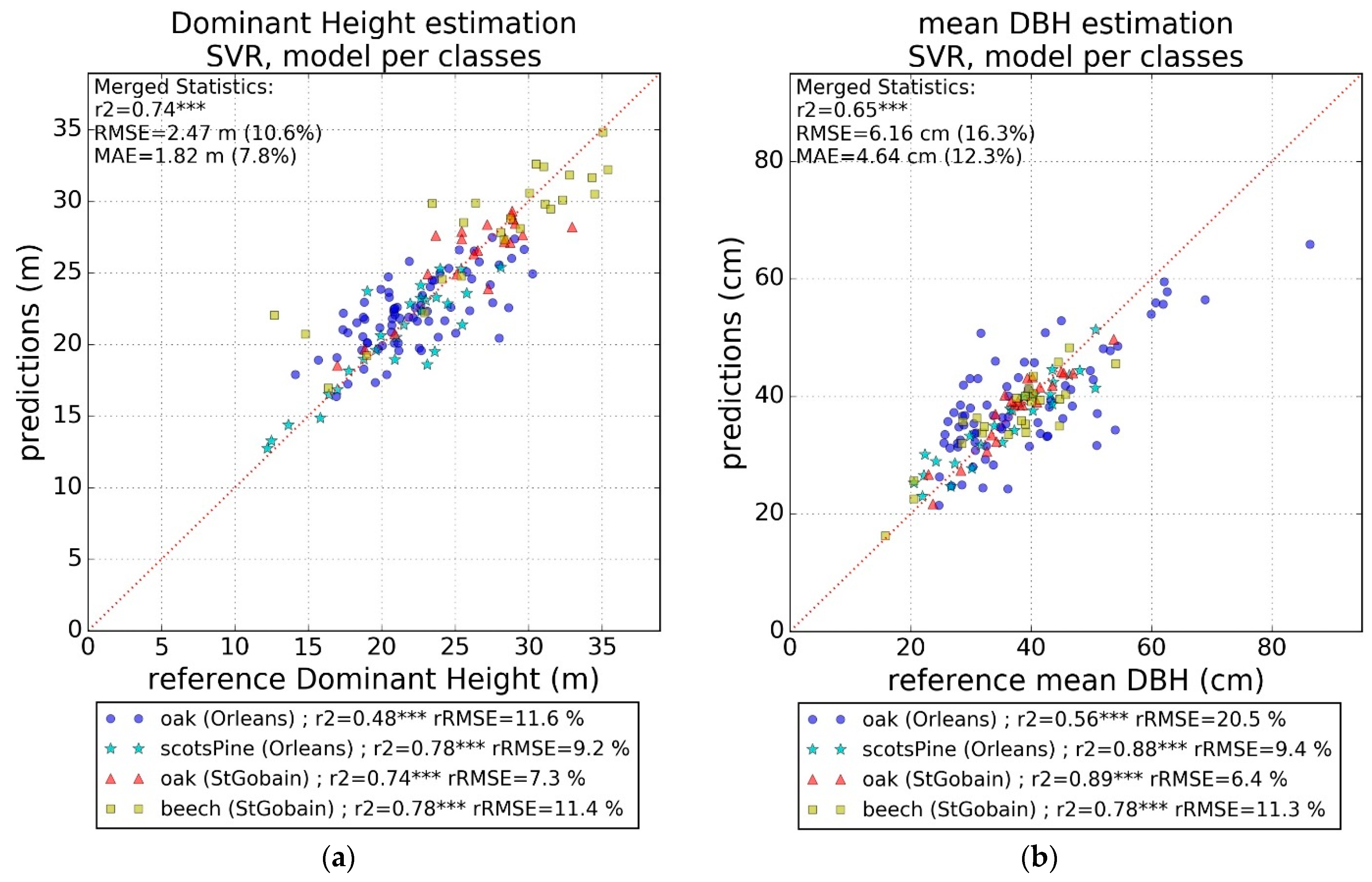
| Hdom (m) | r2 | 0.48 | 0.78 | 0.74 | 0.78 |
| RMSE | 2.56 (11.6%) | 1.92 (9.2%) | 1.90 (7.3%) | 3.10 (11.4%) | |
| MAE | 2.01 (9.1%) | 1.29 (6.2%) | 1.40 (5.4%) | 2.16 (7.9%) | |
| DBH (cm) | r2 | 0.56 | 0.88 | 0.89 | 0.78 |
| RMSE | 7.98 (20.5%) | 3.34 (9.4%) | 2.43 (6.4%) | 4.17 (11.3%) | |
| MAE | 6.56 (16.9%) | 2.56 (7.1%) | 2.06 (5.5%) | 3.41 (9.3%) | |
References
- FAO; UNEP. The State of the World’s Forests 2020. In Forests, Biodiversity and People; FAO: Rome, Italy, 2020. [Google Scholar] [CrossRef]
- FAO. Global Forest Resources Assessment 2020: Main Report; FAO: Rome, Italy, 2020; ISBN 978-92-5-132974-0. [Google Scholar]
- FAO. Global Forest Products Facts and Figures 2018; FAO: Rome, Italy, 2018; p. 20. [Google Scholar]
- Dale, V.H.; Joyce, L.A.; McNulty, S.; Neilson, R.P.; Ayres, M.P.; Flannigan, M.D.; Hanson, P.J.; Irland, L.C.; Lugo, A.E.; Peterson, C.J.; et al. Climate Change and Forest Disturbances: Climate Change Can Affect Forests by Altering the Frequency, Intensity, Duration, and Timing of Fire, Drought, Introduced Species, Insect and Pathogen Outbreaks, Hurricanes, Windstorms, Ice Storms, or Landslides. BioScience 2001, 51, 723–734. [Google Scholar] [CrossRef] [Green Version]
- Jump, A.S.; Peñuelas, J. Running to Stand Still: Adaptation and the Response of Plants to Rapid Climate Change. Ecol. Lett. 2005, 8, 1010–1020. [Google Scholar] [CrossRef] [PubMed]
- Yu, J.; Wang, C.; Wan, J.; Han, S.; Wang, Q.; Nie, S. A Model-Based Method to Evaluate the Ability of Nature Reserves to Protect Endangered Tree Species in the Context of Climate Change. For. Ecol. Manag. 2014, 327, 48–54. [Google Scholar] [CrossRef]
- European Environment Agency. European Forest Ecosystems: State and Trends; Publications Office: Luxembourg, 2016. [Google Scholar]
- Pan, Y.; Birdsey, R.A.; Fang, J.; Houghton, R.; Kauppi, P.E.; Kurz, W.A.; Phillips, O.L.; Shvidenko, A.; Lewis, S.L.; Canadell, J.G.; et al. A Large and Persistent Carbon Sink in the World’s Forests. Science 2011, 333, 988–993. [Google Scholar] [CrossRef] [Green Version]
- French Ministry for the Ecological and Solidary Transition. National Low Carbon Strategy; French Ministry for the Ecological and Solidary Transition: Paris, France, 2020. [Google Scholar]
- Chen, L.; Wang, Y.; Ren, C.; Zhang, B.; Wang, Z. Optimal Combination of Predictors and Algorithms for Forest Above-Ground Biomass Mapping from Sentinel and SRTM Data. Remote Sens. 2019, 11, 414. [Google Scholar] [CrossRef] [Green Version]
- Haywood, A.; Stone, C.; Jones, S. The Potential of Sentinel Satellites for Large Area Aboveground Forest Biomass Mapping. In Proceedings of the IGARSS 2018—2018 IEEE International Geoscience and Remote Sensing Symposium, Valencia, Spain, 23–27 July 2018; pp. 9030–9033. [Google Scholar]
- Laurin, G.V.; Balling, J.; Corona, P.; Mattioli, W.; Papale, D.; Puletti, N.; Rizzo, M.; Truckenbrodt, J.; Urban, M. Above-Ground Biomass Prediction by Sentinel-1 Multitemporal Data in Central Italy with Integration of ALOS2 and Sentinel-2 Data. J. Appl. Remote Sens. 2018, 12, 016008. [Google Scholar] [CrossRef]
- Liu, Y.; Gong, W.; Xing, Y.; Hu, X.; Gong, J. Estimation of the Forest Stand Mean Height and Aboveground Biomass in Northeast China Using SAR Sentinel-1B, Multispectral Sentinel-2A, and DEM Imagery. ISPRS J. Photogramm. Remote Sens. 2019, 151, 277–289. [Google Scholar] [CrossRef]
- Vafaei, S.; Soosani, J.; Adeli, K.; Fadaei, H.; Naghavi, H.; Pham, T.; Tien Bui, D. Improving Accuracy Estimation of Forest Aboveground Biomass Based on Incorporation of ALOS-2 PALSAR-2 and Sentinel-2A Imagery and Machine Learning: A Case Study of the Hyrcanian Forest Area (Iran). Remote Sens. 2018, 10, 172. [Google Scholar] [CrossRef] [Green Version]
- Fassnacht, K.S.; Gower, S.T.; MacKenzie, M.D.; Nordheim, E.V.; Lillesand, T.M. Estimating the Leaf Area Index of North Central Wisconsin Forests Using the Landsat Thematic Mapper. Remote Sens. Environ. 1997, 61, 229–245. [Google Scholar] [CrossRef]
- Melnikova, I.; Awaya, Y.; Saitoh, T.M.; Muraoka, H.; Sasai, T. Estimation of Leaf Area Index in a Mountain Forest of Central Japan with a 30-m Spatial Resolution Based on Landsat Operational Land Imager Imagery: An Application of a Simple Model for Seasonal Monitoring. Remote Sens. 2018, 10, 179. [Google Scholar] [CrossRef] [Green Version]
- Turner, D.P.; Cohen, W.B.; Kennedy, R.E.; Fassnacht, K.S.; Briggs, J.M. Relationships between Leaf Area Index and Landsat TM Spectral Vegetation Indices across Three Temperate Zone Sites. Remote Sens. Environ. 1999, 70, 52–68. [Google Scholar] [CrossRef]
- Castillo-Santiago, M.; Ricker, M.; Jong, B. Estimation of Tropical Forest Structure from SPOT5 Satellite Images. Int. J. Remote Sens. 2010, 31, 2767–2782. [Google Scholar] [CrossRef]
- Freitas, S.R.; Mello, M.C.S.; Cruz, C.B.M. Relationships between Forest Structure and Vegetation Indices in Atlantic Rainforest. For. Ecol. Manag. 2005, 218, 353–362. [Google Scholar] [CrossRef]
- Woodcock, C.E.; Collins, J.B.; Gopal, S.; Jakabhazy, V.D.; Li, X.; Macomber, S.; Ryherd, S.; Judson Harward, V.; Levitan, J.; Wu, Y.; et al. Mapping Forest Vegetation Using Landsat TM Imagery and a Canopy Reflectance Model. Remote Sens. Environ. 1994, 50, 240–254. [Google Scholar] [CrossRef]
- Dong, J.; Kaufmann, R.K.; Myneni, R.B.; Tucker, C.J.; Kauppi, P.E.; Liski, J.; Buermann, W.; Alexeyev, V.; Hughes, M.K. Remote Sensing Estimates of Boreal and Temperate Forest Woody Biomass: Carbon Pools, Sources, and Sinks. Remote Sens. Environ. 2003, 84, 393–410. [Google Scholar] [CrossRef] [Green Version]
- Dube, T.; Mutanga, O. Investigating the Robustness of the New Landsat-8 Operational Land Imager Derived Texture Metrics in Estimating Plantation Forest Aboveground Biomass in Resource Constrained Areas. ISPRS J. Photogramm. Remote Sens. 2015, 108, 12–32. [Google Scholar] [CrossRef]
- Mutanga, O.; Skidmore, A.K. Narrow Band Vegetation Indices Overcome the Saturation Problem in Biomass Estimation. Int. J. Remote Sens. 2004, 25, 3999–4014. [Google Scholar] [CrossRef]
- Proisy, C.; Couteron, P.; Fromard, F. Predicting and Mapping Mangrove Biomass from Canopy Grain Analysis Using Fourier-Based Textural Ordination of IKONOS Images. Remote Sens. Environ. 2007, 109, 379–392. [Google Scholar] [CrossRef]
- Sarker, L.R.; Nichol, J.E. Improved Forest Biomass Estimates Using ALOS AVNIR-2 Texture Indices. Remote Sens. Environ. 2011, 115, 968–977. [Google Scholar] [CrossRef]
- Wolter, P.T.; Townsend, P.A.; Sturtevant, B.R. Estimation of Forest Structural Parameters Using 5 and 10 Meter SPOT-5 Satellite Data. Remote Sens. Environ. 2009, 113, 2019–2036. [Google Scholar] [CrossRef]
- Zhu, X.; Liu, D. Improving Forest Aboveground Biomass Estimation Using Seasonal Landsat NDVI Time-Series. ISPRS J. Photogramm. Remote Sens. 2015, 102, 222–231. [Google Scholar] [CrossRef]
- Austin, J.M.; Mackey, B.G.; Van Niel, K.P. Estimating Forest Biomass Using Satellite Radar: An Exploratory Study in a Temperate Australian Eucalyptus Forest. For. Ecol. Manag. 2003, 176, 575–583. [Google Scholar] [CrossRef]
- Baghdadi, N.; Maire, G.L.; Bailly, J.; Osé, K.; Nouvellon, Y.; Zribi, M.; Lemos, C.; Hakamada, R. Evaluation of ALOS/PALSAR L-Band Data for the Estimation of Eucalyptus Plantations Aboveground Biomass in Brazil. IEEE J. Sel. Top. Appl. Earth Obs. Remote Sens. 2015, 8, 3802–3811. [Google Scholar] [CrossRef] [Green Version]
- Dobson, M.C.; Ulaby, F.T.; Pierce, L.E.; Sharik, T.L.; Lin, C.; Sarabandi, K. Estimation of Forest Biophysical Characteristics in Northem Michigan with SIR-C/X-SAR. IEEE Trans. Geosci. Remote Sens. 1995, 33, 19. [Google Scholar] [CrossRef]
- Le Toan, T.; Beaudoin, A.; Riom, J.; Guyon, D. Relating Forest Biomass to SAR Data. IEEE Trans. Geosci. Remote Sens. 1992, 30, 403–411. [Google Scholar] [CrossRef]
- Mermoz, S.; Le Toan, T.; Villard, L.; Réjou-Méchain, M.; Seifert-Granzin, J. Biomass Assessment in the Cameroon Savanna Using ALOS PALSAR Data. Remote Sens. Environ. 2014, 155, 109–119. [Google Scholar] [CrossRef]
- Santoro, M.; Eriksson, L.; Fransson, J. Reviewing ALOS PALSAR Backscatter Observations for Stem Volume Retrieval in Swedish Forest. Remote Sens. 2015, 7, 4290–4317. [Google Scholar] [CrossRef] [Green Version]
- Attarchi, S.; Gloaguen, R. Improving the Estimation of Above Ground Biomass Using Dual Polarimetric PALSAR and ETM+ Data in the Hyrcanian Mountain Forest (Iran). Remote Sens. 2014, 6, 3693–3715. [Google Scholar] [CrossRef] [Green Version]
- Chen, L.; Ren, C.; Zhang, B.; Wang, Z.; Xi, Y. Estimation of Forest Above-Ground Biomass by Geographically Weighted Regression and Machine Learning with Sentinel Imagery. Forests 2018, 9, 582. [Google Scholar] [CrossRef] [Green Version]
- Gao, T.; Zhu, J.; Deng, S.; Zheng, X.; Zhang, J.; Shang, G.; Huang, L. Timber Production Assessment of a Plantation Forest: An Integrated Framework with Field-Based Inventory, Multi-Source Remote Sensing Data and Forest Management History. Int. J. Appl. Earth Obs. Geoinf. 2016, 52, 155–165. [Google Scholar] [CrossRef]
- Morin, D.; Planells, M.; Guyon, D.; Villard, L.; Mermoz, S.; Bouvet, A.; Thevenon, H.; Dejoux, J.-F.; Le Toan, T.; Dedieu, G. Estimation and Mapping of Forest Structure Parameters from Open Access Satellite Images: Development of a Generic Method with a Study Case on Coniferous Plantation. Remote Sens. 2019, 11, 1275. [Google Scholar] [CrossRef] [Green Version]
- Morin, D.; Planelis, M.; Guyett, D.; Viiiard, L.; Dedieu, G. Estimation of Forest Parameters Combining Multisensor High Resolution Remote Sensing Data. In Proceedings of the IGARSS 2018—2018 IEEE International Geoscience and Remote Sensing Symposium, Valencia, Spain, 23–27 July 2018; pp. 8801–8804. [Google Scholar]
- Chave, J.; Davies, S.J.; Phillips, O.L.; Lewis, S.L.; Sist, P.; Schepaschenko, D.; Armston, J.; Baker, T.R.; Coomes, D.; Disney, M.; et al. Ground Data Are Essential for Biomass Remote Sensing Missions. Surv. Geophys. 2019, 40, 863–880. [Google Scholar] [CrossRef]
- Smith, W.B. Forest Inventory and Analysis: A National Inventory and Monitoring Program. Environ. Pollut. 2002, 116, S233–S242. [Google Scholar] [CrossRef]
- Goedickemeier, I.; Wildi, O.; Kienast, F. Sampling for vegetation survey: Some properties of a gis-based stratification compared to other statistical sampling methods. Coenoses 1997, 12, 43–50. [Google Scholar]
- Jochem, A.; Hollaus, M.; Rutzinger, M.; Höfle, B. Estimation of Aboveground Biomass in Alpine Forests: A Semi-Empirical Approach Considering Canopy Transparency Derived from Airborne LiDAR Data. Sensors 2010, 11, 278–295. [Google Scholar] [CrossRef] [PubMed] [Green Version]
- Yu, X.; Hyyppä, J.; Karjalainen, M.; Nurminen, K.; Karila, K.; Vastaranta, M.; Kankare, V.; Kaartinen, H.; Holopainen, M.; Honkavaara, E.; et al. Comparison of Laser and Stereo Optical, SAR and InSAR Point Clouds from Air- and Space-Borne Sources in the Retrieval of Forest Inventory Attributes. Remote Sens. 2015, 7, 15933–15954. [Google Scholar] [CrossRef] [Green Version]
- Gobakken, T.; Næsset, E.; Nelson, R.; Bollandsås, O.M.; Gregoire, T.G.; Ståhl, G.; Holm, S.; Ørka, H.O.; Astrup, R. Estimating Biomass in Hedmark County, Norway Using National Forest Inventory Field Plots and Airborne Laser Scanning. Remote Sens. Environ. 2012, 123, 443–456. [Google Scholar] [CrossRef]
- d’Oliveira, M.V.N.; Reutebuch, S.E.; McGaughey, R.J.; Andersen, H.-E. Estimating Forest Biomass and Identifying Low-Intensity Logging Areas Using Airborne Scanning Lidar in Antimary State Forest, Acre State, Western Brazilian Amazon. Remote Sens. Environ. 2012, 124, 479–491. [Google Scholar] [CrossRef]
- Bouvier, M.; Durrieu, S.; Fournier, R.A.; Renaud, J.-P. Generalizing Predictive Models of Forest Inventory Attributes Using an Area-Based Approach with Airborne LiDAR Data. Remote Sens. Environ. 2015, 156, 322–334. [Google Scholar] [CrossRef]
- Holopainen, M.; Vastaranta, M.; Karjalainen, M.; Karila, K.; Kaasalainen, S.; Honkavaara, E.; Hyyppä, J. Forest inventory attribute estimation using airborne laser scanning, aerial stereo imagery, radargrammetry and interferometry–finnish experiences of the 3d techniques. ISPRS Ann. Photogramm. Remote Sens. Spat. Inf. Sci. 2015, II-3/W4, 63–69. [Google Scholar] [CrossRef] [Green Version]
- Vastaranta, M.; Holopainen, M.; Karjalainen, M.; Kankare, V.; Hyyppa, J.; Kaasalainen, S. TerraSAR-X Stereo Radargrammetry and Airborne Scanning LiDAR Height Metrics in Imputation of Forest Aboveground Biomass and Stem Volume. IEEE Trans. Geosci. Remote Sens. 2014, 52, 1197–1204. [Google Scholar] [CrossRef]
- Vastaranta, M.; Wulder, M.A.; White, J.C.; Pekkarinen, A.; Tuominen, S.; Ginzler, C.; Kankare, V.; Holopainen, M.; Hyyppä, J.; Hyyppä, H. Airborne Laser Scanning and Digital Stereo Imagery Measures of Forest Structure: Comparative Results and Implications to Forest Mapping and Inventory Update. Can. J. Remote Sens. 2013, 39, 382–395. [Google Scholar] [CrossRef]
- Baghdadi, N.; le Maire, G.; Fayad, I.; Bailly, J.S.; Nouvellon, Y.; Lemos, C.; Hakamada, R. Testing Different Methods of Forest Height and Aboveground Biomass Estimations From ICESat/GLAS Data in Eucalyptus Plantations in Brazil. IEEE J. Sel. Top. Appl. Earth Obs. Remote Sens. 2014, 7, 290–299. [Google Scholar] [CrossRef] [Green Version]
- El Hajj, M.; Baghdadi, N.; Labrière, N.; Bailly, J.-S.; Villard, L. Mapping of Aboveground Biomass in Gabon. Comptes Rendus Géoscience 2019, 351, 321–331. [Google Scholar] [CrossRef]
- Fayad, I.; Baghdadi, N.; Bailly, J.-S.; Barbier, N.; Gond, V.; Hérault, B.; El Hajj, M.; Fabre, F.; Perrin, J. Regional Scale Rain-Forest Height Mapping Using Regression-Kriging of Spaceborne and Airborne LiDAR Data: Application on French Guiana. Remote Sens. 2016, 8, 240. [Google Scholar] [CrossRef] [Green Version]
- Fayad, I.; Baghdadi, N.; Bailly, J.-S.; Barbier, N.; Gond, V.; Hajj, M.E.; Fabre, F.; Bourgine, B. Canopy Height Estimation in French Guiana with LiDAR ICESat/GLAS Data Using Principal Component Analysis and Random Forest Regressions. Remote Sens. 2014, 6, 11883–11914. [Google Scholar] [CrossRef] [Green Version]
- Lefsky, M.A.; Harding, D.J.; Keller, M.; Cohen, W.B.; Carabajal, C.C.; Espirito-Santo, F.D.B.; Hunter, M.O.; de Oliveira, R. Estimates of Forest Canopy Height and Aboveground Biomass Using ICESat. Geophys. Res. Lett. 2005, 32, 4. [Google Scholar] [CrossRef] [Green Version]
- Pourrahmati, M.R.; Baghdadi, N.; Darvishsefat, A.A.; Namiranian, M.; Fayad, I.; Bailly, J.-S.; Gond, V. Capability of GLAS/ICESat Data to Estimate Forest Canopy Height and Volume in Mountainous Forests of Iran. IEEE J. Sel. Top. Appl. Earth Obs. Remote Sens. 2015, 8, 5246. [Google Scholar] [CrossRef] [Green Version]
- Sun, G.; Ranson, K.; Kimes, D.; Blair, J.; Kovacs, K. Forest Vertical Structure from GLAS: An Evaluation Using LVIS and SRTM Data. Remote Sens. Environ. 2008, 112, 107–117. [Google Scholar] [CrossRef]
- Yu, Y.; Yang, X.; Fan, W. Estimates of Forest Structure Parameters from GLAS Data and Multi-Angle Imaging Spectrometer Data. Int. J. Appl. Earth Obs. Geoinf. 2015, 38, 65–71. [Google Scholar] [CrossRef]
- Adam, M.; Urbazaev, M.; Dubois, C.; Schmullius, C. Accuracy Assessment of GEDI Terrain Elevation and Canopy Height Estimates in European Temperate Forests: Influence of Environmental and Acquisition Parameters. Remote Sens. 2020, 12, 3948. [Google Scholar] [CrossRef]
- Dorado-Roda, I.; Pascual, A.; Godinho, S.; Silva, C.; Botequim, B.; Rodríguez-Gonzálvez, P.; González-Ferreiro, E.; Guerra-Hernández, J. Assessing the Accuracy of GEDI Data for Canopy Height and Aboveground Biomass Estimates in Mediterranean Forests. Remote Sens. 2021, 13, 2279. [Google Scholar] [CrossRef]
- Fayad, I.; Ienco, D.; Baghdadi, N.; Gaetano, R.; Alvares, C.A.; Stape, J.L.; Ferraço Scolforo, H.; Le Maire, G. A CNN-Based Approach for the Estimation of Canopy Heights and Wood Volume from GEDI Waveforms. Remote Sens. Environ. 2021, 265, 112652. [Google Scholar] [CrossRef]
- Fayad, I.; Baghdadi, N.N.; Alvares, C.A.; Stape, J.L.; Bailly, J.S.; Scolforo, H.F.; Zribi, M.; Maire, G.L. Assessment of GEDI’s LiDAR Data for the Estimation of Canopy Heights and Wood Volume of Eucalyptus Plantations in Brazil. IEEE J. Sel. Top. Appl. Earth Obs. Remote Sens. 2021, 14, 7095–7110. [Google Scholar] [CrossRef]
- Verhelst, K.; Gou, Y.; Herold, M.; Reiche, J. Improving Forest Baseline Maps in Tropical Wetlands Using GEDI-Based Forest Height Information and Sentinel-1. Forests 2021, 12, 1374. [Google Scholar] [CrossRef]
- Chi, H.; Sun, G.; Huang, J.; Guo, Z.; Ni, W.; Fu, A. National Forest Aboveground Biomass Mapping from ICESat/GLAS Data and MODIS Imagery in China. Remote Sens. 2015, 7, 5534–5564. [Google Scholar] [CrossRef] [Green Version]
- Nelson, R.; Ranson, K.J.; Sun, G.; Kimes, D.S.; Kharuk, V.; Montesano, P. Estimating Siberian Timber Volume Using MODIS and ICESat/GLAS. Remote Sens. Environ. 2009, 113, 691–701. [Google Scholar] [CrossRef]
- Chi, H.; Sun, G.; Huang, J.; Li, R.; Ren, X.; Ni, W.; Fu, A. Estimation of Forest Aboveground Biomass in Changbai Mountain Region Using ICESat/GLAS and Landsat/TM Data. Remote Sens. 2017, 9, 707. [Google Scholar] [CrossRef] [Green Version]
- Duncanson, L.I.; Niemann, K.O.; Wulder, M.A. Integration of GLAS and Landsat TM Data for Aboveground Biomass Estimation. Can. J. Remote Sens. 2010, 36, 129–141. [Google Scholar] [CrossRef]
- Hansen, M.C.; Potapov, P.V.; Goetz, S.J.; Turubanova, S.; Tyukavina, A.; Krylov, A.; Kommareddy, A.; Egorov, A. Mapping Tree Height Distributions in Sub-Saharan Africa Using Landsat 7 and 8 Data. Remote Sens. Environ. 2016, 185, 221–232. [Google Scholar] [CrossRef] [Green Version]
- Liu, K.; Wang, J.; Zeng, W.; Song, J. Comparison and Evaluation of Three Methods for Estimating Forest above Ground Biomass Using TM and GLAS Data. Remote Sens. 2017, 9, 341. [Google Scholar] [CrossRef] [Green Version]
- Wang, M.; Sun, R.; Xiao, Z. Estimation of Forest Canopy Height and Aboveground Biomass from Spaceborne LiDAR and Landsat Imageries in Maryland. Remote Sens. 2018, 10, 344. [Google Scholar] [CrossRef] [Green Version]
- Zhang, G.; Ganguly, S.; Nemani, R.R.; White, M.A.; Milesi, C.; Hashimoto, H.; Wang, W.; Saatchi, S.; Yu, Y.; Myneni, R.B. Estimation of Forest Aboveground Biomass in California Using Canopy Height and Leaf Area Index Estimated from Satellite Data. Remote Sens. Environ. 2014, 151, 44–56. [Google Scholar] [CrossRef]
- Fayad, I.; Baghdadi, N.; Alvares, C.A.; Stape, J.L.; Bailly, J.S.; Scolforo, H.F.; Zribi, M.; Le Maire, G. Estimating Canopy Height and Wood Volume of Eucalyptus Plantations in Brazil Using GEDI LiDAR Data. In Proceedings of the 2021 IEEE International Geoscience and Remote Sensing Symposium IGARSS, Brussels, Belgium, 11–16 July 2021; pp. 5941–5944. [Google Scholar]
- Potapov, P.; Li, X.; Hernandez-Serna, A.; Tyukavina, A.; Hansen, M.C.; Kommareddy, A.; Pickens, A.; Turubanova, S.; Tang, H.; Silva, C.E.; et al. Mapping Global Forest Canopy Height through Integration of GEDI and Landsat Data. Remote Sens. Environ. 2021, 253, 112165. [Google Scholar] [CrossRef]
- Chen, L.; Ren, C.; Zhang, B.; Wang, Z.; Liu, M.; Man, W.; Liu, J. Improved Estimation of Forest Stand Volume by the Integration of GEDI LiDAR Data and Multi-Sensor Imagery in the Changbai Mountains Mixed Forests Ecoregion (CMMFE), Northeast China. Int. J. Appl. Earth Obs. Geoinf. 2021, 100, 102326. [Google Scholar] [CrossRef]
- Global Forest Canopy Height. 2019. Available online: https://glad.umd.edu/dataset/gedi (accessed on 16 March 2022).
- Morin, D. Estimation et Suivi de la Ressource en Bois en France Métropolitaine par Valorisation des Séries Multi-Temporelles à Haute Résolution Spatiale D’images Optiques (Sentinel-2) et Radar (Sentinel-1, ALOS-PALSAR). Ph.D. Thesis, Université Paul Sabatier-Toulouse III, Toulouse, France, 2020. [Google Scholar]
- Krebs, M.; Piboule, A. Computree. Available online: http://computree.onf.fr (accessed on 16 March 2022).
- Piboule, A.; Krebs, M.; Esclatine, L.; Hervé, J.C. Computree: A Collaborative Platform for Use of Terrestrial Lidar in Dendrometry. In Proceedings of the International IUFRO Conference MeMoWood, Nancy, France, 1–4 October 2013. [Google Scholar]
- Theia Land Data Center. Available online: https://theia.cnes.fr (accessed on 16 March 2022).
- Hagolle, O.; Huc, M.; Pascual, D.V.; Dedieu, G. A Multi-Temporal Method for Cloud Detection, Applied to FORMOSAT-2, VENµS, LANDSAT and SENTINEL-2 Images. Remote Sens. Environ. 2010, 114, 1747–1755. [Google Scholar] [CrossRef] [Green Version]
- Hagolle, O.; Huc, M.; Villa Pascual, D.; Dedieu, G. A Multi-Temporal and Multi-Spectral Method to Estimate Aerosol Optical Thickness over Land, for the Atmospheric Correction of FormoSat-2, LandSat, VENμS and Sentinel-2 Images. Remote Sens. 2015, 7, 2668–2691. [Google Scholar] [CrossRef] [Green Version]
- PEPS, Plateforme d’exploitation des produits Sentinel. Available online: https://peps.cnes.fr (accessed on 16 March 2022).
- Bruniquel, J.; Lopes, A. Multi-Variate Optimal Speckle Reduction in SAR Imagery. Int. J. Remote Sens. 1997, 18, 603–627. [Google Scholar] [CrossRef]
- Quegan, S.; Yu, J.J. Filtering of Multichannel SAR Images. IEEE Trans. Geosci. Remote Sens. 2001, 39, 2373–2379. [Google Scholar] [CrossRef]
- Shimada, M.; Ohtaki, T. Generating Large-Scale High-Quality SAR Mosaic Datasets: Application to PALSAR Data for Global Monitoring. IEEE J. Sel. Top. Appl. Earth Obs. Remote Sens. 2010, 3, 637–656. [Google Scholar] [CrossRef]
- Grizonnet, M.; Michel, J.; Poughon, V.; Inglada, J.; Savinaud, M.; Cresson, R. Orfeo ToolBox: Open Source Processing of Remote Sensing Images. Open Geospat. Data Softw. Stand. 2017, 2, 15. [Google Scholar] [CrossRef] [Green Version]
- Dubayah, R.; Blair, J.B.; Goetz, S.; Fatoyinbo, L.; Hansen, M.; Healey, S.; Hofton, M.; Hurtt, G.; Kellner, J.; Luthcke, S.; et al. The Global Ecosystem Dynamics Investigation: High-Resolution Laser Ranging of the Earth’s Forests and Topography. Sci. Remote Sens. 2020, 1, 100002. [Google Scholar] [CrossRef]
- Khati, U.; Lavalle, M.; Singh, G. The Role of Time-Series L-Band SAR and GEDI in Mapping Sub-Tropical Above-Ground Biomass. Front. Earth Sci. 2021, 9, 752254. [Google Scholar] [CrossRef]
- Inglada, J.; Vincent, A.; Arias, M.; Tardy, B.; Morin, D.; Rodes, I. Operational High Resolution Land Cover Map Production at the Country Scale Using Satellite Image Time Series. Remote Sens. 2017, 9, 95. [Google Scholar] [CrossRef] [Green Version]
- López, N.S. Validation de L’estimation de la Hauteur des Jeunes Peuplements à Partir de Données LiDAR Aériennes. Ph.D. Thesis, Université de Lorraine, Metz, France, 2013. [Google Scholar]
- Lucie, X.; Durrieu, S.; Jolly, A.; Labbé, S.; Renaud, J.-P. Comparaison de Modèles Numériques de Surface photogrammétriques de différentes résolutions en forêt mixte. estimation d’une variable dendrométrique simple: La hauteur dominante. Rev. Française Photogrammétrie Télédétection 2017, 213, 143–151. [Google Scholar] [CrossRef]
- Pearse, G.D.; Dash, J.P.; Persson, H.J.; Watt, M.S. Comparison of High-Density LiDAR and Satellite Photogrammetry for Forest Inventory. ISPRS J. Photogramm. Remote Sens. 2018, 142, 257–267. [Google Scholar] [CrossRef]


| Orléans | StGobain | |||
|---|---|---|---|---|
| Oak | Scots Pine | Oak | Beech | |
| Plot number | 75 | 28 | 21 | 25 |
| Hdom (m) | 22.1 ± 3.6 | 20.8 ± 4.0 | 26.2 ± 3.7 | 27.3 ± 6.2 |
| BA (m2/ha) | 18.0 ± 5.8 | 20.8 ± 8.3 | 21.0 ± 8.8 | 19.1 ± 9.2 |
| DBH (cm) | 38.8 ± 12.0 | 35.8 ± 8.8 | 37.7 ± 7.2 | 36.8 ± 8.8 |
| Density (tree/ha) | 164 ± 85 | 237 ± 133 | 155 ± 68 | 153 ± 66 |
| Site | Orléans | StGobain | |||
|---|---|---|---|---|---|
| Class (Plots) | Oak (75) | Scots Pine (28) | Oak (21) | Beech (25) | |
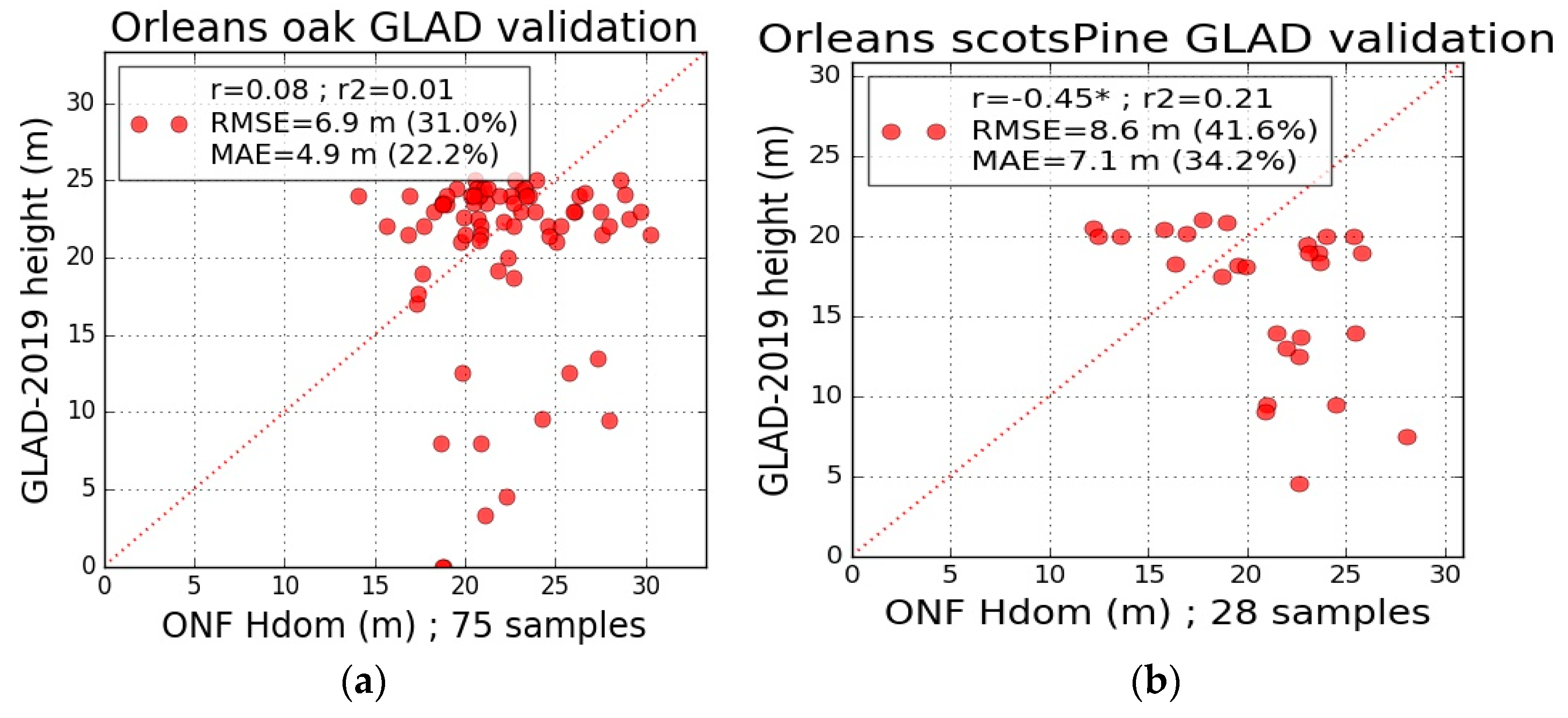
| GLAD-2019 Test ONF | r2 | 0.01 | 0.21 | 0.21 | 0.1 |
| RMSE | 6.9 (31.0%) | 8.6 (41.6%) | 3.9 (14.8%) | 6.6 (24.3%) | |
| MAE | 4.9 (22.2%) | 7.1 (34.2%) | 3.3 (12.8%) | 5.9 (21.5%) | |
| Train ONF/RSdata Test ONF | r2 | 0.48 | 0.78 | 0.74 | 0.78 |
| RMSE | 2.6 (11.6%) | 1.9 (9.2%) | 1.9 (7.3%) | 3.1 (11.4%) | |
| MAE | 2.0 (9.1%) | 1.3 (6.2%) | 1.4 (5.4%) | 2.2 (7.9%) | |
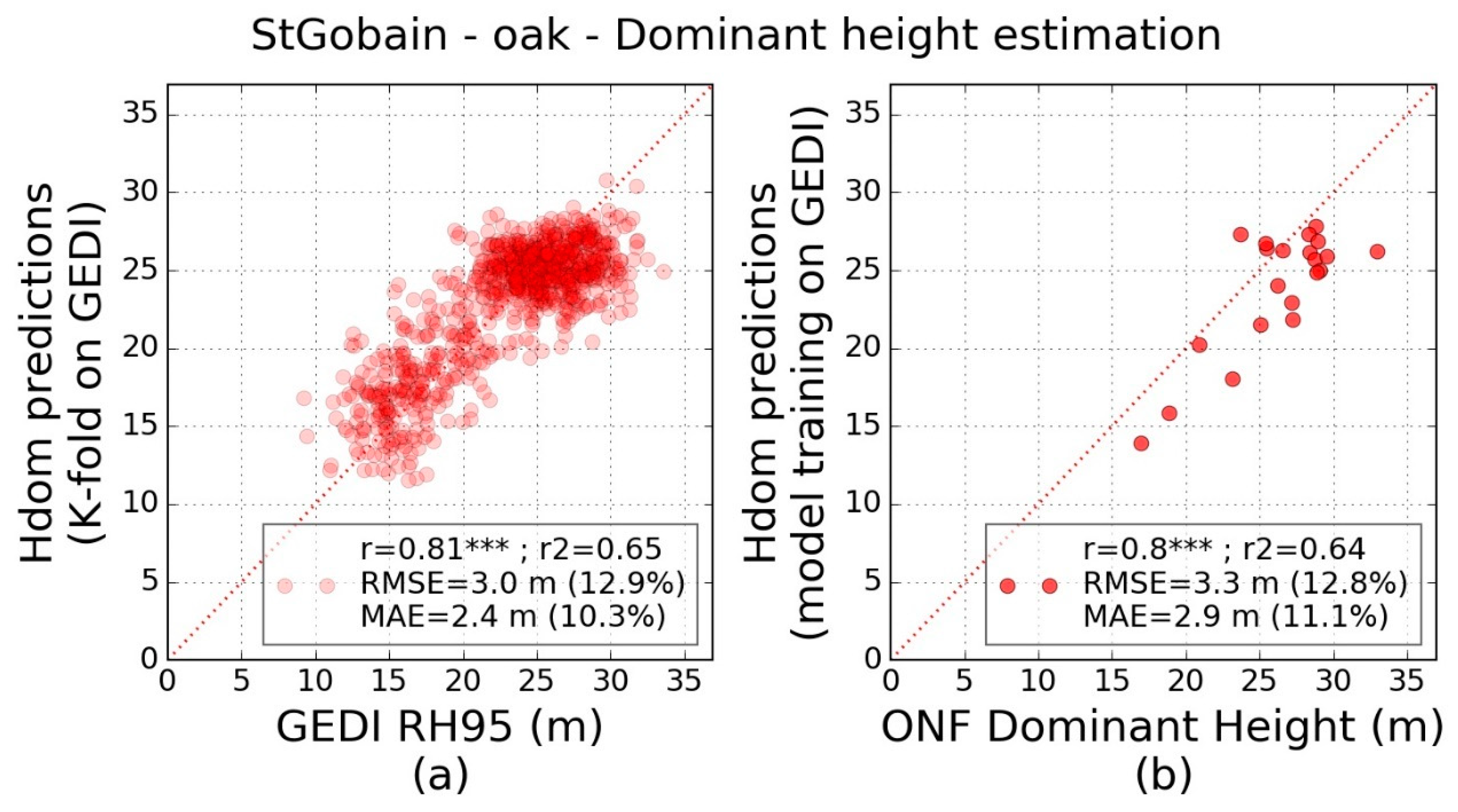
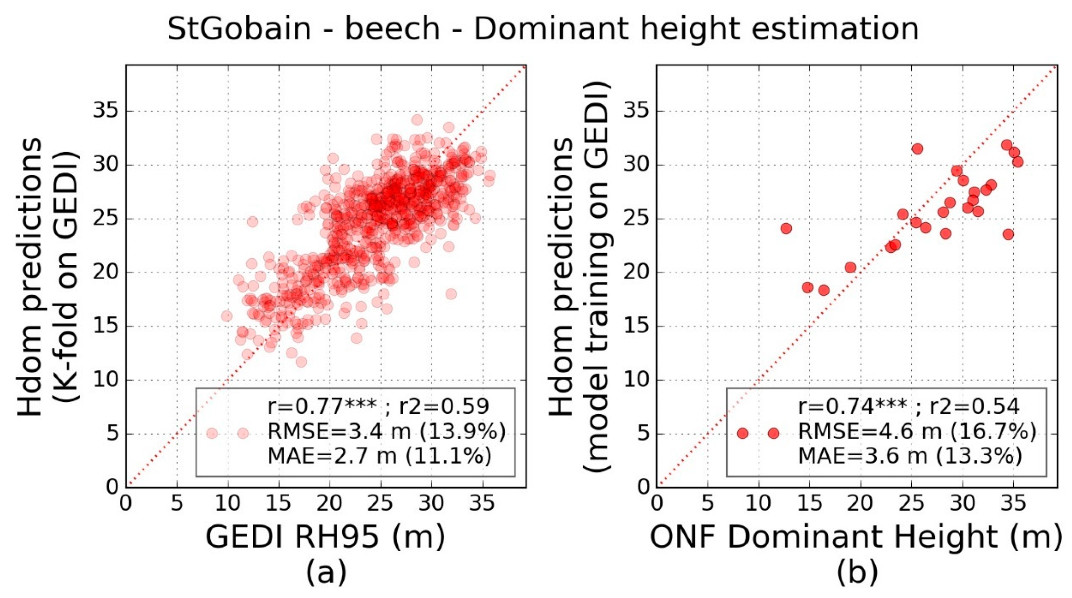
| Train GEDI/RSdata Test ONF | r2 | 0.23 | 0.55 | 0.64 | 0.54 |
| RMSE | 3.3 (14.7%) | 3.0 (14.3%) | 3.3 (12.8%) | 4.6 (16.7%) | |
| MAE | 2.7 (12.4%) | 2.4 (11.3%) | 2.9 (11.1%) | 3.6 (13.3%) | |
| Train GEDI/RSdata Test GEDI | Class (footprints) | Oak (479) | Scots pine (958) | Oak (808) | Beech (723) |
| r2 | 0.54 | 0.64 | 0.65 | 0.59 | |
| RMSE | 3.4 (16.7%) | 2.7 (15.5%) | 2.9 (12.9%) | 3.4 (13.9%) | |
| MAE | 2.6 (12.9%) | 2.2 (12.2%) | 2.4 (10.3%) | 2.7 (11.1%) | |
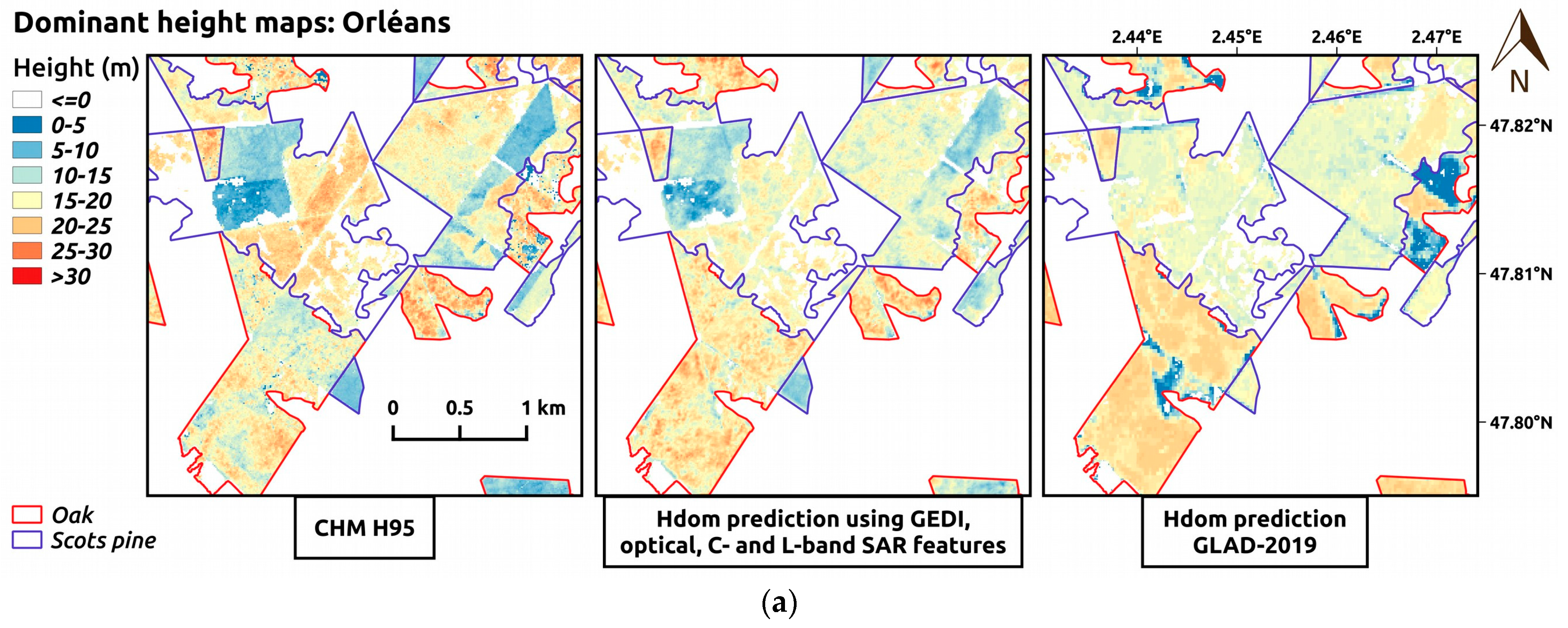
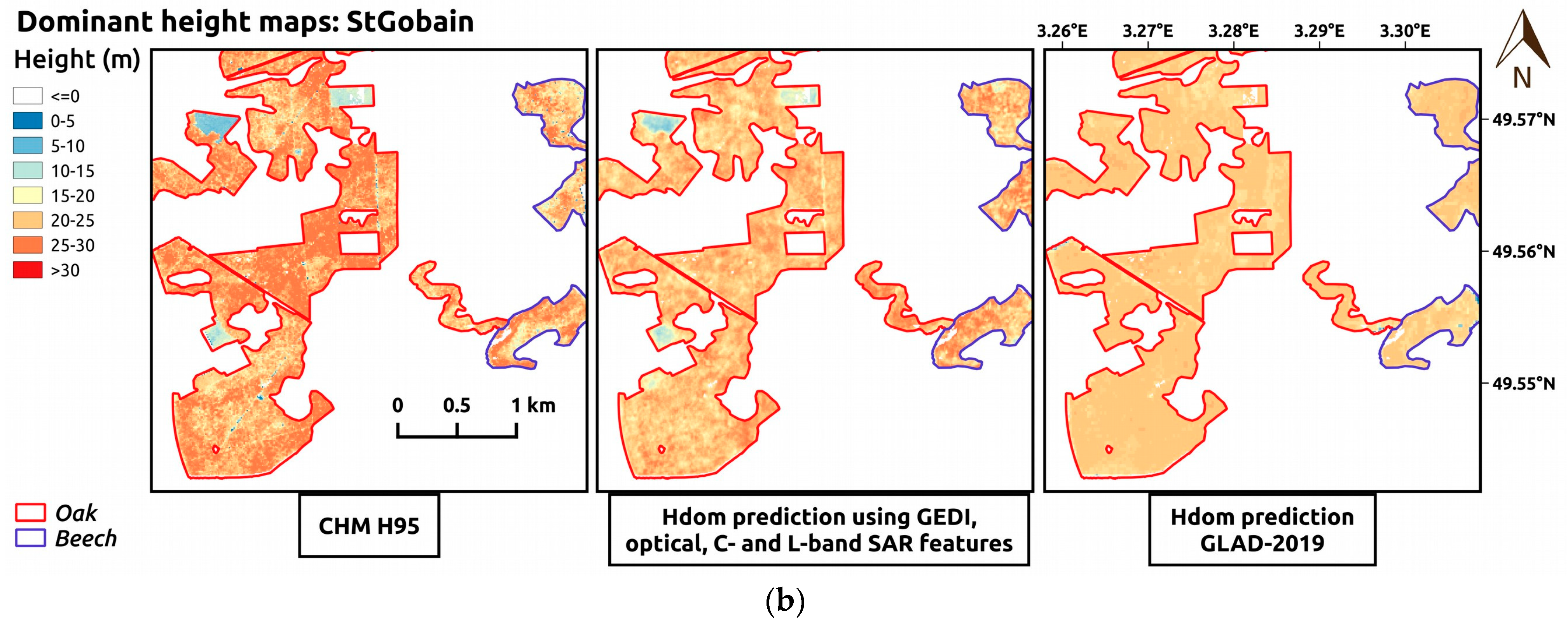
| Maps comparison: Train GEDI/RSdata Test CHM-H95 | Class (pixels) | Oak (149,165) | Scots pine (168,031) | Oak (113,916) | Beech (107,213) |
| r2 | 0.49 | 0.57 | 0.56 | 0.47 | |
| RMSE | 4.5 (22.9%) | 3.5 (19.2%) | 4.0 (16.9%) | 4.8 (19.0%) | |
| MAE | 3.6 (18.3%) | 2.8 (15.1%) | 3.2 (13.4%) | 3.8 (14.9%) | |
Publisher’s Note: MDPI stays neutral with regard to jurisdictional claims in published maps and institutional affiliations. |
© 2022 by the authors. Licensee MDPI, Basel, Switzerland. This article is an open access article distributed under the terms and conditions of the Creative Commons Attribution (CC BY) license (https://creativecommons.org/licenses/by/4.0/).
Share and Cite
Morin, D.; Planells, M.; Baghdadi, N.; Bouvet, A.; Fayad, I.; Le Toan, T.; Mermoz, S.; Villard, L. Improving Heterogeneous Forest Height Maps by Integrating GEDI-Based Forest Height Information in a Multi-Sensor Mapping Process. Remote Sens. 2022, 14, 2079. https://0-doi-org.brum.beds.ac.uk/10.3390/rs14092079
Morin D, Planells M, Baghdadi N, Bouvet A, Fayad I, Le Toan T, Mermoz S, Villard L. Improving Heterogeneous Forest Height Maps by Integrating GEDI-Based Forest Height Information in a Multi-Sensor Mapping Process. Remote Sensing. 2022; 14(9):2079. https://0-doi-org.brum.beds.ac.uk/10.3390/rs14092079
Chicago/Turabian StyleMorin, David, Milena Planells, Nicolas Baghdadi, Alexandre Bouvet, Ibrahim Fayad, Thuy Le Toan, Stéphane Mermoz, and Ludovic Villard. 2022. "Improving Heterogeneous Forest Height Maps by Integrating GEDI-Based Forest Height Information in a Multi-Sensor Mapping Process" Remote Sensing 14, no. 9: 2079. https://0-doi-org.brum.beds.ac.uk/10.3390/rs14092079