Article

Integration of VIIRS Observations with GEDI-Lidar Measurements to Monitor Forest Structure Dynamics from 2013 to 2020 across the Conterminous United States

1
Department of Geographical Sciences, University of Maryland, College Park, MD 20742, USA
2
U.S. Forest Service, 507-25th Street, Ogden, UT 84401, USA
3
NOAA-NESDIS Center for Satellite Applications and Research (STAR), 5830 University Research Court, College Park, MD 20740, USA
*
Author to whom correspondence should be addressed.
Remote Sens. 2022, 14(10), 2320; https://0-doi-org.brum.beds.ac.uk/10.3390/rs14102320
Submission received: 14 March 2022 / Revised: 7 May 2022 / Accepted: 7 May 2022 / Published: 11 May 2022
(This article belongs to the Special Issue Forest Monitoring in a Multi-Sensor Approach)

Abstract

:
Consistent and spatially explicit periodic monitoring of forest structure is essential for estimating forest-related carbon emissions, analyzing forest degradation, and supporting sustainable forest management policies. To date, few products are available that allow for continental to global operational monitoring of changes in canopy structure. In this study, we explored the synergy between the NASA’s spaceborne Global Ecosystem Dynamics Investigation (GEDI) waveform LiDAR and the Visible Infrared Imaging Radiometer Suite (VIIRS) data to produce spatially explicit and consistent annual maps of canopy height (CH), percent canopy cover (PCC), plant area index (PAI), and foliage height diversity (FHD) across the conterminous United States (CONUS) at a 1-km resolution for 2013–2020. The accuracies of the annual maps were assessed using forest structure attribute derived from airborne laser scanning (ALS) data acquired between 2013 and 2020 for the 48 National Ecological Observatory Network (NEON) field sites distributed across the CONUS. The root mean square error (RMSE) values of the annual canopy height maps as compared with the ALS reference data varied from a minimum of 3.31-m for 2020 to a maximum of 4.19-m for 2017. Similarly, the RMSE values for PCC ranged between 8% (2020) and 11% (all other years). Qualitative evaluations of the annual maps using time series of very high-resolution images further suggested that the VIIRS-derived products could capture both large and “more” subtle changes in forest structure associated with partial harvesting, wind damage, wildfires, and other environmental stresses. The methods developed in this study are expected to enable multi-decadal analysis of forest structure and its dynamics using consistent satellite observations from moderate resolution sensors such as VIIRS onboard JPSS satellites.

1. Introduction

Human activities and natural processes are rapidly changing the global distribution and 3-dimensional (3-D) structure of forests [1,2]. These changes have broad impacts on earth system processes and the sustainability and diversity of living organisms [3,4]. Monitoring changes in forest structure is crucial for advancing research related to carbon and biogeochemical cycles [5,6], ecosystem functioning [7], and biological conservation [8].
While much is known about the diversity of vegetation structure and species composition in North American forests [2,9], datasets are still needed to characterize the rates of change in forest structure, carbon flux, and stock dynamics [10,11]. For example, the degradation of forest stocks from selective logging, low-severity disturbances, and the regeneration rates of forests following a disturbance remains poorly characterized at the scales needed for assessing carbon dynamics, water quality and quantity, and other environmental goods and services [10,12]. Accurate estimates of the 3-D distribution of vegetation structure and their changes over time are thus of critical importance in studies of global environmental change and terrestrial biodiversity as well as in numerical weather and water predictions [11,13,14,15].
A major challenge to monitoring changes in forest structure from optical and radar data at continental to global scales has been the difficulty of obtaining high-quality, globally representative training samples. The high costs and logistic burdens associated with collecting needed training data using ground-based methods are unbearable for any individual project or organization. The deployment of the GEDI-LiDAR instrument on the International Space Station (ISS) in late 2018 [11] greatly improved the sampling of global forests using LiDAR [16,17]. GEDI is the first space-borne, full-waveform LiDAR that was specifically designed to measure ecosystem structure by providing vertical profiles of forest canopies with 25-m footprints on the ground [11]. Since April 2019, the instrument has collected more than 10 billion cloud-free footprints sampling more than 4% of the land surface between 51.6 degrees north and south on a sparse sampling grid.
Signal processing algorithms have been used by the GEDI team to derive from the GEDI waveforms canopy height models and other structural variables including canopy cover, vertical plant area, and foliage height diversity profiles [18,19]. Compared to its first iteration, the second version of the GEDI products released on 16 Apr 2021 has improved geolocation accuracies (20 m for the first version and 10 m for the second version [11]) and provides additional datasets that allow the end-users the flexibility to select the subset of waveforms better suited for their particular application [20].
Measurements from GEDI are limited to samples collected along the laser tracks [11]. GEDI data consist of footprint-based measurements collected between ~51.6°N and ~51.6°S globally, but data coverage is limited by the ISS orbit inclination [16]. Gridded products at the 1-km scale are being produced from the valid footprints within each grid cell [21]. The recent extension of the GEDI mission into 2023 will result in more valid footprints and therefore more representative sampling of vegetation structure within each 1-km2 cell. However, the spatial coverage of the gridded products is incomplete and they will be produced for the mission years only [11,21].
The integration of GEDI footprints with on-orbit optical data (e.g., Landsat, Sentinel, MODIS, VIIRS) could allow for the interpolation of spatially explicit and dense time series of forest structure properties spanning multiple decades [16,22]. A multi-decadal record of forest structural dynamics is especially valuable for understanding how forests respond to disturbances [23,24], how it changes during post-disturbance recovery [25], and the interactions between disturbance, recovery, and climate change [26]. Such a long forest structure record will enable new research aimed at advancing the understanding and protection of global biodiversity [27,28], reducing uncertainties with the global carbon budget [6,10,29,30], and improving model studies of key climate and hydrological processes important to the global environmental system [31].
Together with machine learning algorithms, optical observations from systems like Landsat, MODIS, and VIIRS were used to extrapolate LiDAR measurements to produce spatially contiguous map products for a single year as in [16,32,33,34]. Vegetation cover and canopy height models derived from Airborne Laser Scanning (ALS) data have also been used with Landsat and MODIS data to characterize inter-annual changes in forest cover and tree height in the Lower Mekong region [35] and map multi-decadal changes in forest structure across Canada [36].
While spaceborne GEDI is more sensitive to vegetation 3-D structure than spaceborne optical and radar instruments, the stochasticity in the GEDI waveforms caused by a number of factors including geolocation inaccuracies, digitizer noise, pulse shape, terrain slope, varying atmospheric transmission, and surface reflectance do introduce uncertainties in modeling canopy height and the other canopy structure profiles [37]. Such uncertainties can be characterized using ALS data since ALS data collected during the leaf-on season have been found to provide estimates of forest structure comparable to ground-based measurements [38,39,40,41,42,43,44]. Several studies used ALS data to validate forest structure products derived from space-borne platforms, including canopy height, canopy cover, and height profiles [16,34,37,45,46,47]. The errors in GEDI L2A canopy height product (version 2) were quantified in [47] using contemporaneous high-resolution, locally calibrated ALS-derived canopy height data collected for the National Science Foundation’s National Ecological Observatory Network (NEON) field sites in the U.S. mainland and Hawaii. They found that the GEDI product yields reasonable estimates of canopy height (RMSE 3.56 m) when only the power beam data acquired at night were used. The accuracy was lower RMSE 7.21 m when the NEON ALS data were compared to GEDI data regardless of daytime or beam strength.
In our previous work [22], we demonstrated that machine-learning algorithms can be used to integrate VIIRS observations with GEDI-derived estimates of forest structure to produce spatially explicit, wall-to-wall estimates of canopy fractional cover (CFC), canopy height (CH), plant area index (PAI), and foliage height diversity (FHD) across the CONUS for a single year (2019). In this study, we used a similar approach to produce annual estimates of the same key forest structure attributes across the CONUS for the eight years from 2013–2020. We further characterized the uncertainties of these annual estimates by comparing these estimates with forest structure products calculated from the ALS data collected over the NEON field sites. The specific objectives of the study were:
(i)
to model the relationships between the second release of GEDI data and VIIRS observations collected in 2019 in order to develop a suite of well-calibrated models that can map the four forest structure attributes across the CONUS;
(ii)
to apply the models to the VIIRS archive to produce global forest structure map products on an annual basis from 2013 to 2020;
(iii)
to demonstrate the robustness of the products by validating the resulting forest structural estimates using 2020 GEDI data and independent NEON ALS data acquisitions from 2013 to 2020 that encompass a broad range of forest types and conditions; and
(iv)
to produce a qualitative evaluation of the potential of the annual products to capture changes in forest structure that may rise from disturbance and recovery.
The steps used in this study to produce and evaluate the accuracy of the annual (2013–2020) wall-to-wall forest structure products are shown in Figure 1. The resulting annual suite of calibrated and validated forest structure attributes will be valuable for understanding how forest responds to disturbances and how it changes during post-disturbance recovery.

2. Materials and Methods

2.1. VIIRS Multitemporal Metrics

Daily surface reflectance data from the Suomi National Polar-Orbiting Partnership (Suomi NPP) Visible Infrared Imaging Radiometer Suite (VIIRS) VIIRS sensor were used in this study. Following previous MODIS and VIIRS-based global vegetation and land cover studies [48,49,50,51,52,53], we used surface reflectance data from the nine moderate resolution bands, including M1-M5, M7, M8, M10, and M11. The swath data with a nadir resolution of 750 m were gridded following the MODIS Sinusoidal projection system with a nominal 1-km (~926 m) resolution to create CONUS mosaics. For each year from 2013 to 2020, the 9 M-Bands were processed to create a set of multi-temporal spectral metrics to serve as consistent land surface inputs for mapping 3-D canopy structures. This section provides an overview of VIIRS data processing. More details have been described in previous studies [48,50,53].
The daily VIIRS surface reflectance data were aggregated to create 5-day and 32-day composites using the self-adaptive compositing approach, which employs spectral and temporal information to determine the general surface cover condition (e.g., vegetation/land, water, snow/ice) of a given pixel and adaptively select the most suitable compositing criterion for that pixel [53]. The monthly composited values were used to create the annual spectral metrics using the methods described in [50,54]. Compositing reduces temporal inconsistencies associated with clear-sky data availability, cloud shadow and snow cover contamination [55] and hence may allow more consistent mapping of vegetation structure [48,49,54].
For each year in the data record, the VIIRS-derived annual surface type (2013–2020) [48,50], and the geographic position of each pixel encoded in coordinates of latitude (−90–90°) and longitude (−180–180°) were added to the annual and monthly composite data. The inclusion of geographic position was based on the hypothesis that because large-scale climate patterns exert strong control on the geographic distribution of vegetation biomes, geographic position serves as a good predictor of land cover and vegetation class at continental to global scales [52]. The compositing process resulted in 8 annual multi-temporal metrics representing the surface conditions for each year from 2013 to 2020. Each multi-temporal metrics had 144 variables. The list of variables in every annual multi-temporal metric that were used to produce spatially explicit maps of CH, CFC, PAI, and FHD across the CONUS are listed in Table 1.

2.2. GEDI Data Processing

With an overarching goal to advance the understanding of ecosystem structure and dynamics, GEDI has been optimized for retrieving vegetation vertical structure [11]. It uses waveform LiDAR to sample the Earth’s surface between 51.6°N and 51.6°S from the International Space Station (ISS). The GEDI instrument consists of three lasers: one “coverage” laser and two “full power” lasers. The three lasers produce a total of eight-beam ground transects that are spaced approximately 600 m apart on the Earth’s surface in the cross-track direction. Each beam transect consists of ~25 m footprint samples approximately spaced every 60 m along track.
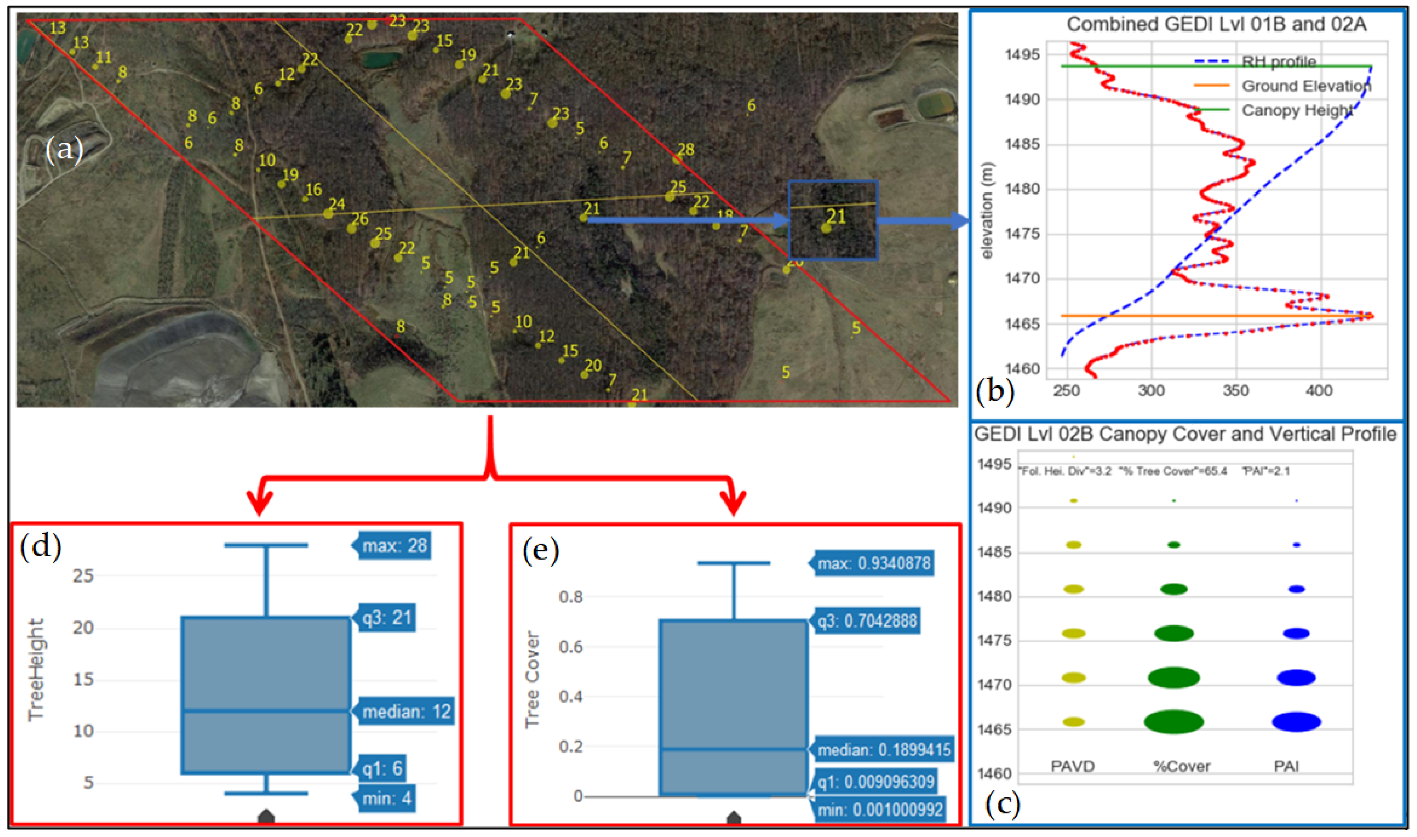
The fundamental footprint observations made by the GEDI instrument are received waveforms of energy as a function of receive time. The valid waveforms are then used in [18,19] to derive the directional gap probability profile and the canopy structure vertical profiles. This suit of GEDI mission standard products (GEDI Level 02B; Version 2 [19]) include CH, CFC, PAI, and FHD derived from the ~25 m footprints. CFC is the percent of the ground covered by the vertical projection of canopy material. CH is canopy top height. PAI is similar to leaf area index but incorporates, in addition to leaves, all other canopy structural elements (e.g., branches and trunks). FHD, also known as Shannon’s diversity index, describes the vertical heterogeneity of foliage profile [56].
Version 2 of the GEDI level 02B product [57] over CONUS were obtained for the period from 18 April 2019 to 31 August 2020. Differences from the first release of the GEDI products include better geolocation for orbital segments, and a modified method to predict an optimum algorithm setting group per laser shot. The obtained data had 855,688,803 GEDI level 02B valid waveforms and footprints of CH, CFC, PAI, and FHD.
The quality of the derived forest structure attributes from GEDI waveforms can vary due to the effects of known (e.g., pulse shape, pulse energy, digitizer noise) and unknown (e.g., atmospheric attenuation, local slope, multiplicative scattering, background solar illumination) factors. These factors affect the accuracy of determining the ranging points along the waveform and thus the quality of forest structure estimates [37]. For example, the GEDI coverage beam waveforms under dense canopy cover conditions may return a weak ground signal that is difficult to detect against high background noise [20]. Waveform “sensitivity” values in the GEDI products provide an estimate for the relative minimum percentage of the waveform energy return that needs to be present in the ground for it to be detected [11,58]. Therefore, in dense forests, only waveforms with high “sensitivity” values have a good probability of detecting the ground ranging point.
To select the highest quality data, we utilized the GEDI quality flags and applied additional selection criteria (Table 2) in order to exclude footprints with poor geolocation performance, poor signal quality, locations with urban structures, and the footprints collected during daytime and during the leaf-off period. A more complete description of the GEDI data products quality flags is provided in [18,19,20]. This selection process retained a subset of 114,790,783 GEDI waveforms or ~13.71% of the data. Of these 63,261,705 waveforms were collected in 2019 and 51,529,078 were collected in 2020. The number of GEDI footprints removed at each step in the filtering process are listed in Table 3.
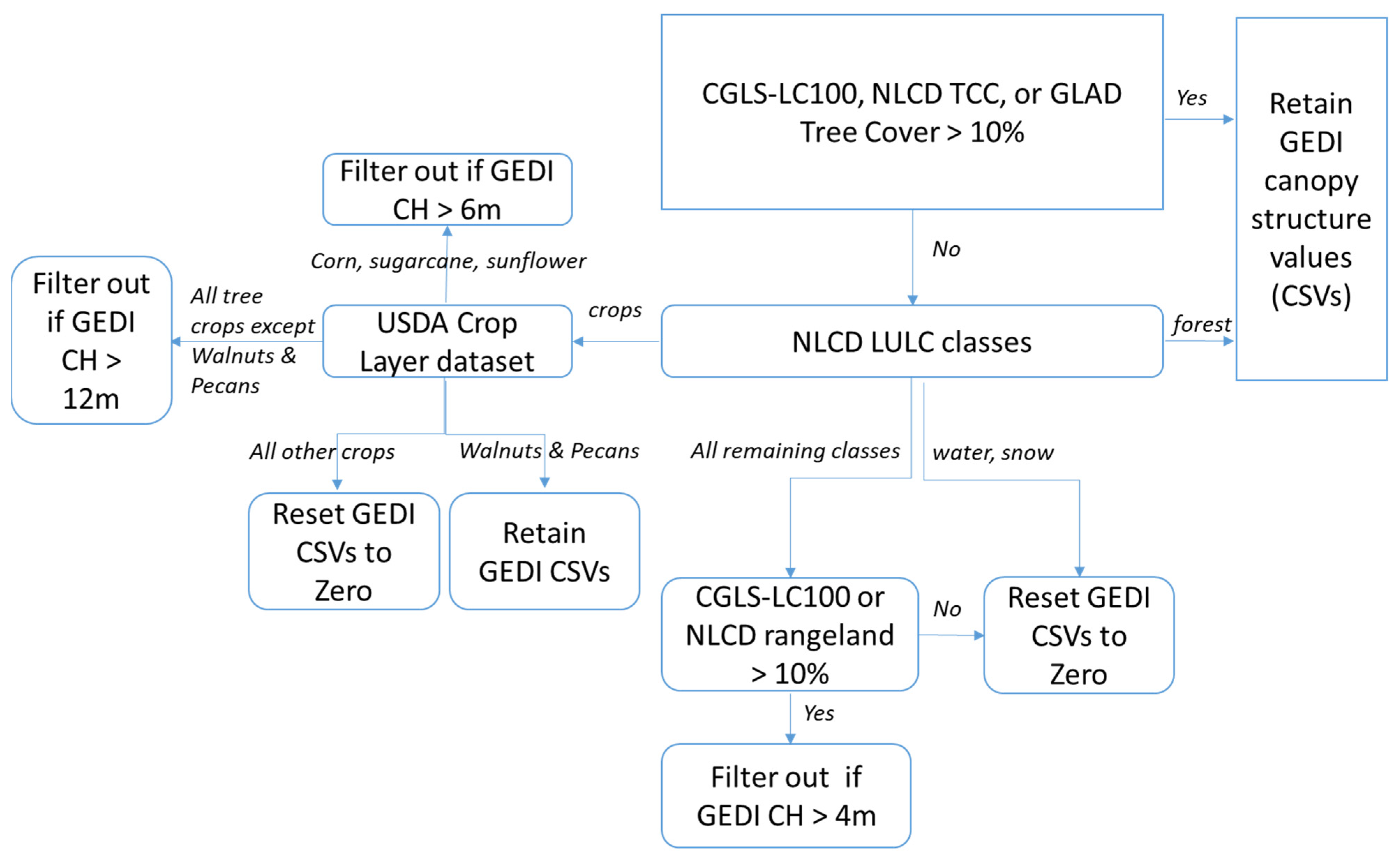
The GEDI vegetation product suite appears to overestimate canopy height over many non-forest areas [16,22]. To address this problem, several available intermediate-scale (30–100 m) land cover products were used to identify GEDI footprints located in areas that have little or no woody vegetation (<10% tree cover) following the rules shown in Figure 2.
We retained all GEDI values located in the grid cells classified by the National Land Cover Database (NLCD-LC 2016) [59] as forests and woody wetlands or had a percentage tree cover value > 10% in any of the three continuous vegetation products used in this study. These were the NLCD 2016 tree canopy cover (TCC) [60], the global land analysis and discovery (GLAD) TCC [61], and the 2019 Copernicus Global Land Cover (CGLS-LC100) [62]. The remaining GEDI footprints that were located in the areas classified by NLCD-LC as water or permanent snow had their canopy structure attributes reset to zero. We then used the 2019 and 2020 United States Department of Agriculture Cropland data layers (USDA-CDL) [63] to interrogate the GEDI-canopy height values in cultivated areas. Tree crops, except Walnuts and Pecans, are often managed not to grow taller than 12 m [64,65,66,67,68,69]. GEDI footprints with TH values >12 m were excluded from further analysis since it is likely that GEDI overestimated tree height in these areas. Tall field crops (e.g., corn, sugarcane, and sunflower) rarely exceed a height of 6 m. We excluded the GEDI footprints from further analysis if the footprint TH value exceeded 6 m. The GEDI values collocated with field crops other than corn, sugarcane, and sunflower were edited to have CH, CFC, PAI, and FHD values reset to zero. Finally, the GEDI-footprints located in barren areas, grasslands and shrub lands with less than 10% shrub cover had their forest structure attributes reset to zero (Figure 2). Out of the 114.8 million GEDI footprints, approximately half of a million were excluded from further analysis due to possible overestimation of vegetation canopy height and 34.7 million GEDI-footprints had their CH, CFC, PAI, and FHD values reset to zero due to being located in areas that had no woody vegetation. Table 4 provides a breakdown of the distribution of GEDI footprints per land cover type, the number of footprints where the GEDI-derived forest structure values were reset to zero and the number of GEDI footprints excluded from further analysis.
The remaining GEDI level 02B footprints collected in 2019 (63,261,705 footprints) were mapped into the VIIRS standard global 1-km Sinusoidal grid system. This resulted in 3.65 million collocated VIIRS–GEDI paired data records. The number of GEDI footprints falling within a collocated VIIRS grid cell ranged between 1 and 157 observations. Of the 3.65 million collocated VIIRS–GEDI paired data records, 2.08 million (or 56.94%) contained 20 or more GEDI footprints whereas only some 150 thousand contained 50 or more GEDI footprints. Table 5 shows the number of VIIRS–GEDI data records with 20+, 30+, 40+, and 50+ collocated GEDI footprints. Generally, a higher number of GEDI footprints within a VIIRS pixel should better represent the variability of canopy structure attributes within that pixel. However, as the cutoff value of collocated GEDI footprints increases, the number of collocated GEDI–VIIRS paired data records decreases exponentially. This is especially the case in dense forests and is a direct result of filtering out the GEDI footprints collected using the coverage beam and the GEDI footprints with sensitivity metric < 0.95. Using high cutoff values could therefore result in an inadequate representation of forest types and conditions, which could in turn affect the ability of the machine learning models to explain the full range of variability in forest conditions across the CONUS.
For each of the datasets (1 through 4) in Table 5, the mean and median values of the GEDI-derived forest structure attributes within the coincident VIIRS grid cells were calculated (Figure 3). This was done in order to investigate the relationships between VIIRS and GEDI data products. The output are metrics of GEDI forest structure attributes paired to their collocated 2019 VIIRS annual metrics data. Henceforth, these are referred to as the 2019 GEDI–VIIRS paired data records.
The distributions of the GEDI–VIIRS paired data records in Table 5 under samples forests (forests were estimated in [48,59] to cover ~26% of the CONUS land area) and oversamples grasslands and croplands. According to NLCD [59], grasslands and croplands cover ~46% of the CONUS land area, whereas 65% or more of the GEDI–VIIRS paired data records are located in these land cover classes.
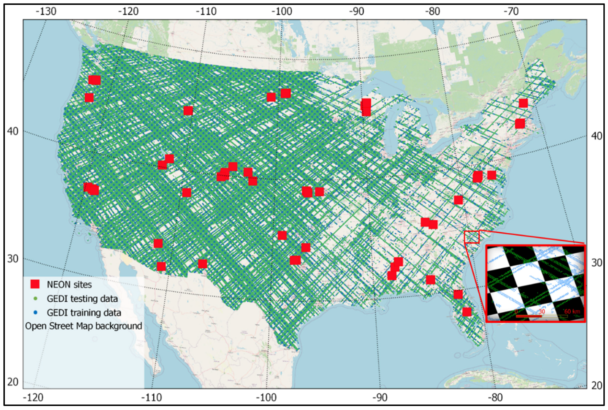
To reduce the impacts of sub-optimal sampling on modeling forest structure attributes from VIIRS data, the LiDAR –VIIRS paired data records were randomly subsampled to obtain a distribution that matches that of the land cover classes in NLCD 2016 (Table 6). The GEDI–VIIRS paired data records were then split into equally sized training and testing subsets using a 25-km checkerboard grid (Figure 4). Selecting spatially disaggregated training and testing data should reduce the impacts of spatial autocorrelation on model validation results [44,52].
The same data processing procedures applied to the 2019 GEDI data were then applied to the 2020 GEDI level 02B footprints. The 51,529,078 footprints were mapped into the VIIRS standard global 1-km Sinusoidal grid system. This resulted in 2.71 million collocated VIIRS–GEDI paired data records. The 2020 GEDI–VIIRS paired data records were then subsampled to obtain a distribution that matches that for the NLCD land cover classes. The VIIRS–GEDI paired data records were then subset into training and testing data using the same checkerboard approach applied to the 2019 GEDI–VIIRS paired data records.

2.3. NEON ALS Data

The National Science Foundation’s National Ecological Observatory Network (NEON) is a US-wide observation network with its sites strategically located across the U.S. to capture variability in ecological and climatological conditions [70] (see also Figure 4). The network spans a wide range of terrestrial ecosystems from shrublands to forests (Table 7). Airborne LiDAR surveys were conducted over NEON field sites during peak greenness to provide ecosystem three-dimensional structural information. The LiDAR sensors are typically flown at an altitude of 1000 m above ground level (AGL) and operated at a pulse return frequency PRF between 100 and 400 kHz. At these PRFs, 2–8 laser pulses per square meter will typically intercept the landscape. If the ground cover produces multiple returns, a point density of up to 64 points per square meter can be obtained. In areas where flight lines overlap, the number of pulses or points can be higher.
The NEON Level 1 Discrete Return LiDAR Point Cloud data product [71] was obtained for the 48 NEON sites across the CONUS. Since 2013, Airborne LiDAR surveys were carried over most NEON sites three or more times. Each airborne survey covered an area of 100–300 km2. The number of airborne surveys across the CONUS averaged 5 surveys per year for the period 2013–2015. Since 2016, the average number of surveys sharply increased to 30 surveys/year (Table 8).
Pertinent information in the NEON LiDAR point cloud data include the projected location and elevation above Geoid for each point in the cloud as well as the relative signal intensity, point return number, and point classification (‘ground’, ‘vegetation’, ‘building’, ‘noise’ and ‘unclassified’).
The classified NEON LiDAR data were obtained in tiles measuring 1 km by 1 km in the compressed LAZ format. The tiles from each airborne survey were decompressed and merged into one file in LAS format using the LAStools software suite [72]. ALS data were then processed using the GEDI simulator software suite [58] to simulate GEDI waveforms and to derive canopy height models, canopy cover, PAI and FHD vertical profiles. The GEDI simulator was described in detail and validated in [58]. Waveforms are simulated following the methods proposed in [73]. The waveforms simulated from discrete return LiDAR were compared to observed large-footprint LiDAR over dense tropical forests [73]. It was found that the method could accurately recreate the waveform shapes. As long as the ALS data are of sufficient pulse density (greater than 3 pulses/m2), the simulated RH metrics, compared to collocated LVIS (Land, Vegetation, and Ice Sensor) LiDAR waveforms, was found in [58] to have less than 0.22 m bias.
The GEDI waveforms were simulated from the ALS points classified as ground and canopy. The classified points were used to distinguish the ground and canopy portions of the waveform. This is required for estimating canopy cover, plant area index, and foliage height diversity [74]. The parameters for simulating the GEDI waveforms from ALS points are given in Table 9. The GEDI system pulse was assumed to be near Gaussian and defined by the full-width half-maximum of the Gaussian (FWHM = 15.6 ns) as in [58]. In simulating the GEDI waveforms, the ALS points were normalized for ALS point density and weighted by the number of hits each beam records (weight  =  1/number of hits), which assumes that each hit along a laser beam intersects a surface of equal area, as used in [74].
The waveform may contain several distinct modes representing reflecting surfaces within each footprint. The modes in the on-orbit GEDI waveforms are detected at the zero crossing points of the first derivative of the de-noised data [18]. To process the ALS-simulated waveforms, we similarly selected, in the GEDI simulator, the zero-crossing point of the first derivative for the detection of the ranging points. The waveforms and the detected modes are then used to calculate canopy relative height (RH) metrics, canopy cover fraction (CCF), plant area index (PAI), and foliage height diversity (FHD) as described in [
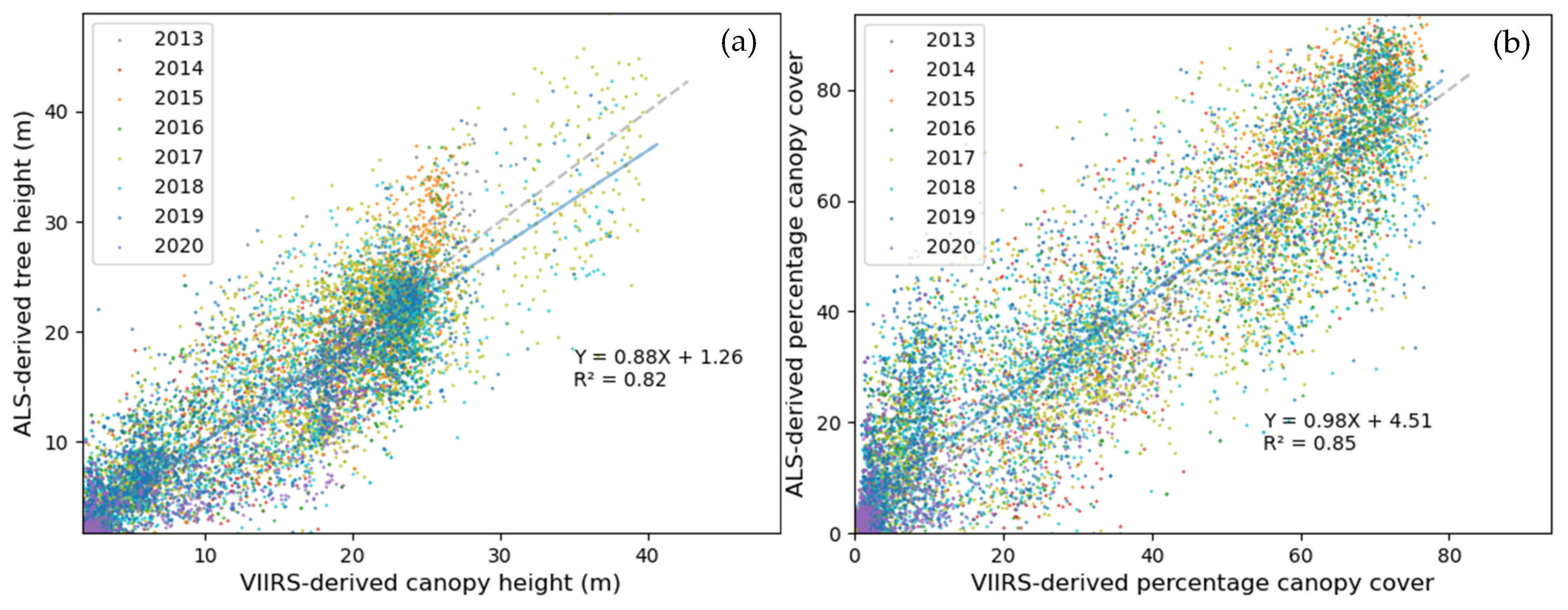
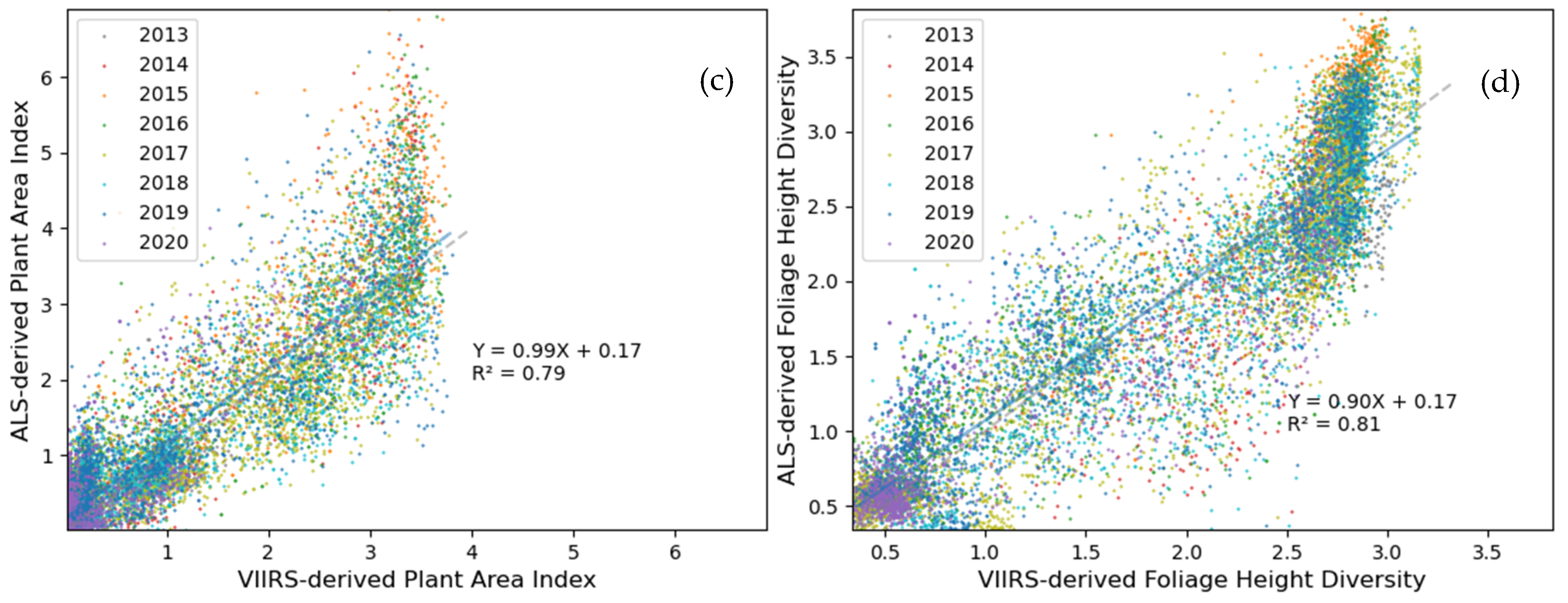
19,58]. The simulations resulted in 25-m spatially explicit grids of forest structure attributes for all the NEON sites across the CONUS. The ALS-derived grids were then collocated with their contemporaneous VIIRS pixels. Statistical summaries (mean, median, count, and standard deviation) were then calculated from the ALS-derived data for each collocated VIIRS pixel. This dataset will be used for the validation of the VIIRS-derived wall-to-wall forest structure maps (see Section 2.5).

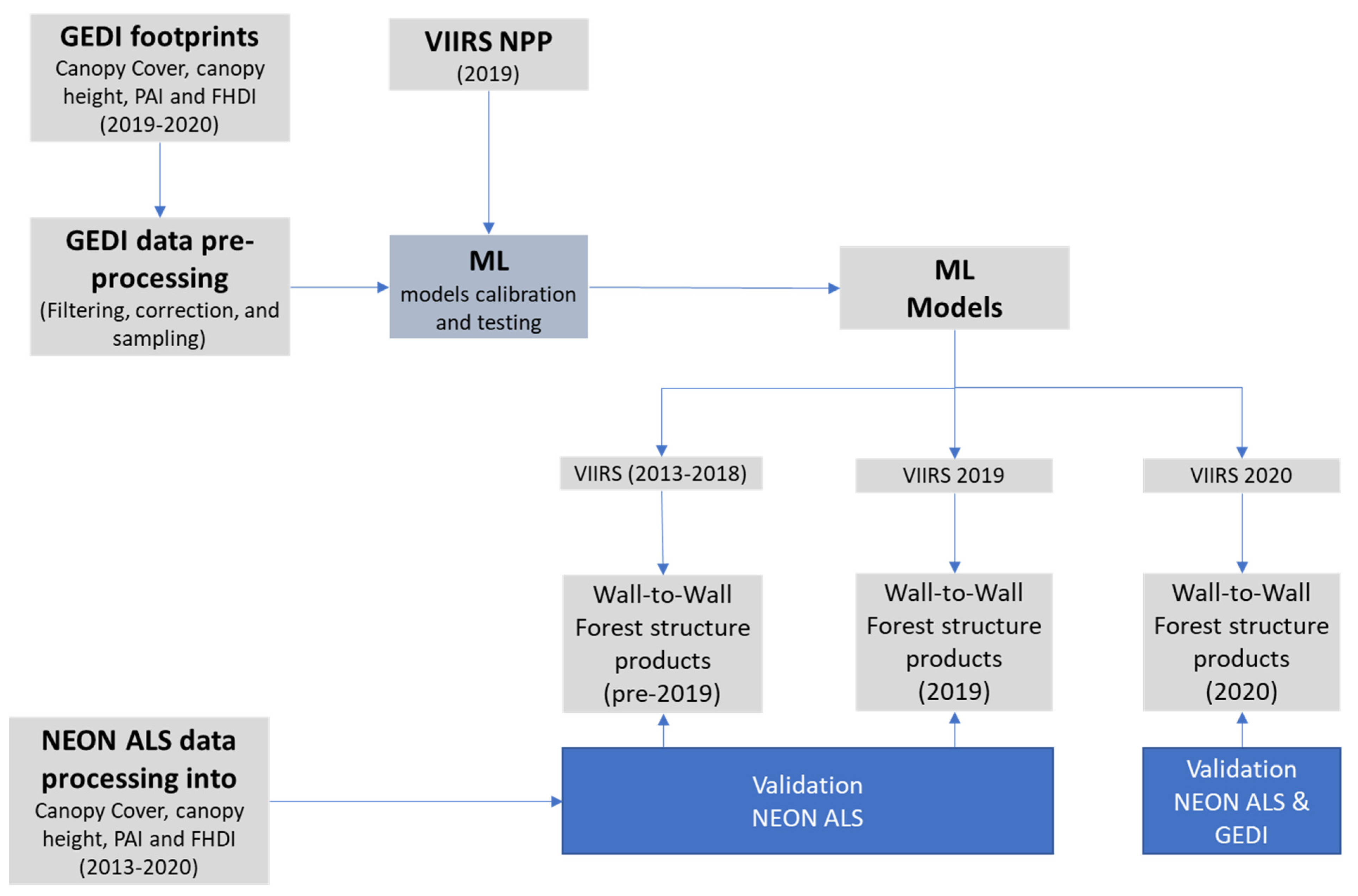
2.4. Forest Structure Mapping

The training subset from the 2019 GEDI–VIIRS paired data records (Table 6, Section 2.2) was used to train random forest regression models [75] that can predict GEDI-like CH, CFC, PAI, and FHD. In total, VIIRS-derived multi-temporal metrics containing 144 variables (Table 1, Section 2.1) were used as input features (i.e., independent variables) in model construction.
Random forest regression models are ensemble machine learning methods [75]. Random forests grow a user-defined number of regression trees and averages their predictions. In random forests, each tree in the ensemble (i.e., forest) is built from a sample drawn with replacement (i.e., a bootstrap sample). Furthermore, when splitting each node in a tree, the best split is found either from all input features or from a random subset of features [76]. The size of the subset of features and other regression tree model hyperparameters (e.g., number of trees in the forest, the maximum depth of the regression trees, etc.) that produce optimal model performance were evaluated in [22]. The values of the optimal random forest hyper-parameters used in [22] were also used in this study.
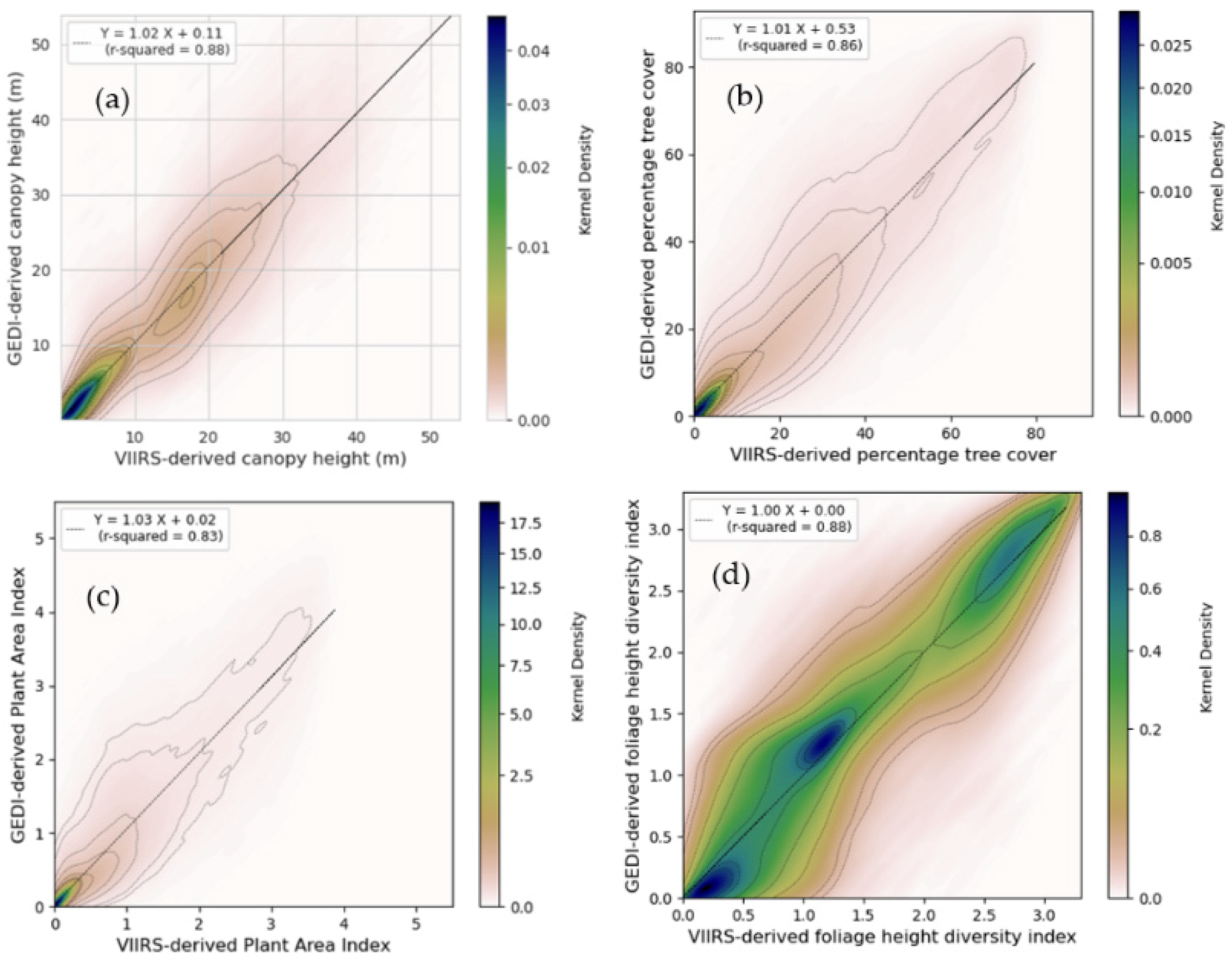
The random forest (RF) regression models that can predict the GEDI-like CH, CFC, PAI, and FHD were calibrated using the training subsets obtained from the VIIRS–GEDI paired data records listed in 
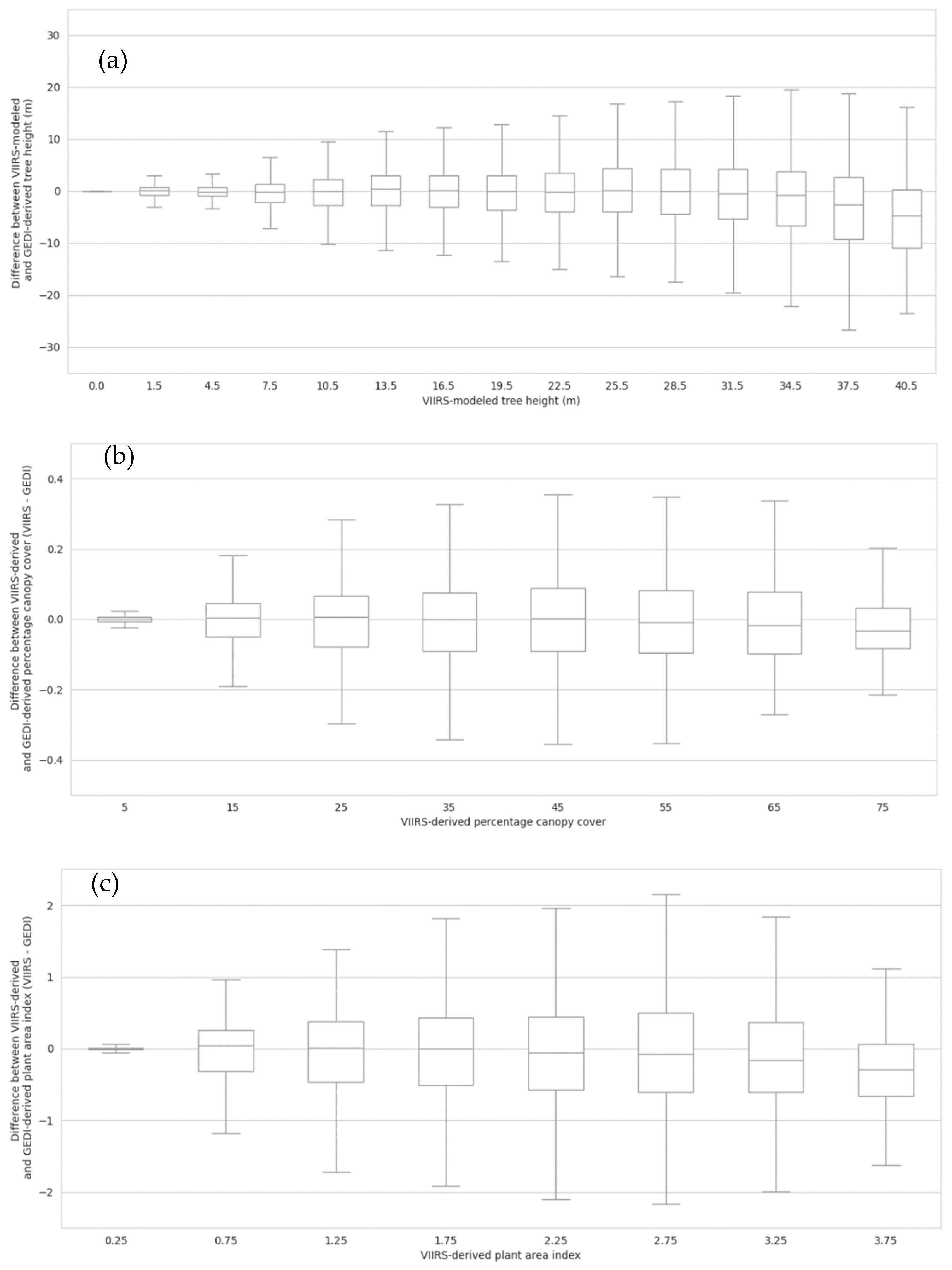
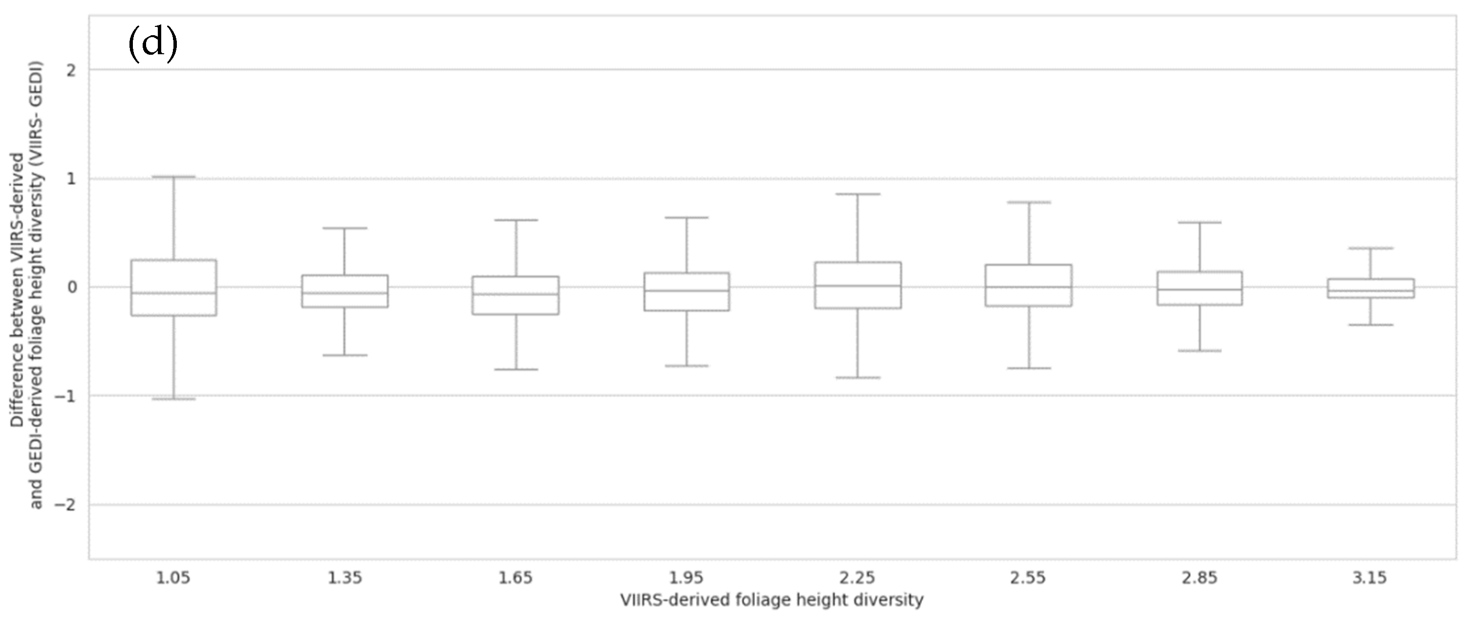
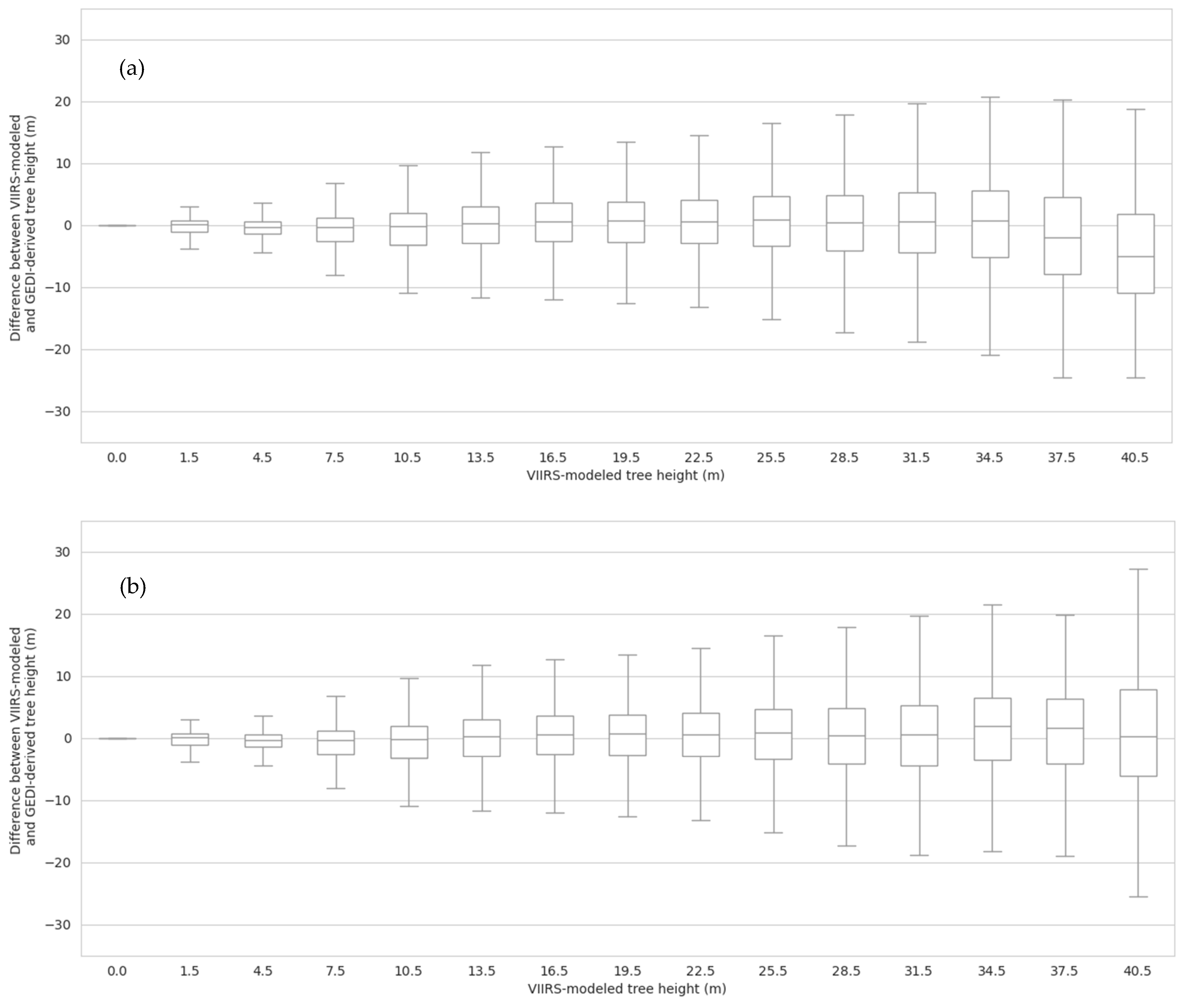
Table 6. In total, 16 RF models were trained (four models per forest structure attribute). The VIIRS–GEDI paired data records testing subsets were used to evaluate the ability of the 16 models to explain the variances observed in the GEDI-derived canopy structural elements (R squared values as a measure of the precision of the models). The evaluation criteria used included the mean and median absolute errors (MAE, and MDAE; respectively), as well as the root-mean-squared error (RMSE) values calculated from the differences between the GEDI and VIIRS predicted forest structure attributes. We also investigated model bias by calculating the distribution of differences between model-derived canopy structural elements and their corresponding GEDI-derived values at multiple intervals of each variable’s distribution. Because the training samples are not located near the testing samples (see Section 2.3), the risk of the derived accuracy assessments being overestimated due to spatial autocorrelations between training and testing samples should be low [52,77].
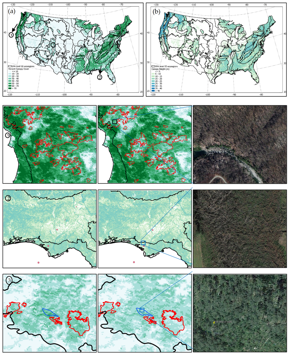
Based on the model evaluation criteria, the “better” performing models were applied to the VIIRS metrics in order to produce annual (2013–2020) wall-to-wall maps of canopy height, fraction canopy cover, plant area index, and foliage height diversity for the conterminous US. In producing the wall-to-wall maps, water bodies were not processed since the GEDI data used in model calibration did not include observations over water. The 926.65-m grid size water mask was calculated from the global 231.66-m land/water product [78]. Any 926.65-m pixel was flagged as a water pixel if any of the 16 spatially coincident pixels in the original product were classified as water pixels.

2.5. Validation of the Generated Products

The VIIRS-derived products should be consistent over time to allow monitoring of changes in forest structure that result from natural growth, disturbance, and post-disturbance recovery. In order for the products to be consistent over time, a key requirement is that the VIIRS observations are consistent. Thanks to long-term, careful and systematic calibration and monitoring efforts [79], the VIIRS–NPP have produced highly consistent surface reflectance products since 2013 [80]. Therefore, the RF models developed by the integration of GEDI and VIIRS observations should allow the derivation of consistent annual forest structure products back to 2013 when the earliest complete annual VIIRS observation record became available.
We quantify the quality and consistency of the mapped products using: (1) the independent ALS-derived forest structure attributes (see Section 2.3); (2) the 2020 GEDI validation dataset (see Section 2.2); and (3) qualitatively by contrasting the annual profiles of VIIRS-derived forest structure attributes with known disturbance events and annual visual interpretations of very high-resolution aerial images. The criteria for the quantitative assessments were the same used in Section 2.4; namely r2, RMSE, MAE, and MDAE.
The NEON ALS data were used to quantify the overall quality of the VIIRS products and to produce annual assessments for the years 2016 to 2020. There were only five NEON ALS campaigns per year for the years 2013 to 2015. The small size of the validation sample from 2013 to 2015 could not therefore be used to produce annual assessments. Rather, the ALS data collected over the 3-year period were used to produce an aggregate assessment of the accuracy of the VIIRS products for 2013–2015. Compared to the ALS data, the on-orbit 2020 GEDI testing dataset greatly improves the spatial representativeness of the validation results.

3. Results

3.1. Development and Evaluation of Random Forest Models

The 2019 GEDI–VIIRS paired data records (Table 6, Section 2.2) were used to train random forest regression models that can predict GEDI-like forest structure attributes across the CONUS from the wall-to-wall VIIRS observations. The reserved 2019 GEDI test data (see Section 2.2) were used to evaluate the ability of these models to reproduce the GEDI-derived CH, CFC, PAI, and FHD values.
Model evaluation results are summarized in Table 9. The RF models trained with 30+ coincident GEDI footprints per VIIRS pixel slightly outperformed the RF models trained with 20+ coincident GEDI footprints per VIIRS pixel. However, using higher thresholds (40+) of coincident GEDI footprints per VIIRS pixel, in general, did not improve the models’ performance while using a 50+ threshold reduced the ability of the models to explain the variance in the test GEDI data (Table 9). Furthermore, the GEDI–VIIRS data records with 40+ and 50+ collocated GEDI observations appeared to under-sample dense canopies across the CONUS. Therefore, the RF models trained using the 2019 GEDI–VIIRS paired data records that contained 30+ coincident GEDI footprints per VIIRS pixel were selected to map the four forest structure attributes across the CONUS.
When calculated over the entire data range, comparisons between the 2019 GEDI test data and the collocated 2019 VIIRS-mapped values had negligible bias and offset values (Figure 5). Boxplots were used to investigate the distribution of the differences between the VIIRS and the GEDI values at different intervals representing the range of canopy height values. The RF canopy height model underestimated GEDI-derived canopy height data for tall (>33 m) trees (Figure 6a). Similarly, the Plant Area Index model underestimated the GEDI-derived Plant Area Index at index values greater than 3 (Figure 6c). Underestimation of fraction tree cover in denser forests was less pronounced, while the comparisons of FHD values showed good correspondence between the modeled and reference data for all strata (Figure 6b,d).
To correct for the underestimation of the VIIRS-derived CH values, we divide the GEDI-derived CH values into 1-m bins. The mean GEDI-derived and their corresponding VIIRS-derived CH values were calculated for each bin. A scatter plot (Figure S1, Supplementary Material) between the two sets of mean CH values revealed a piecewise relationship with: (1) a near-perfect 1:1 relationship for CH values < 33 m (GEDI mean CH = VIIRS mean CH + 0.09 m, r2 = 1); and (2) a linear underestimation of GEDI mean CH (GEDI mean CH = 1.5 × VIIRS mean CH −16.12 m, r2 = 0.93) for CH values ≥ 33 m. These linear relationships were then applied to the wall-to-wall maps to correct for the underestimation in GEDI-derived CH values. By adjusting the VIIRS-derived CH values using these linear functions, most of the biases between the VIIRS and GEDI-derived mean CH values were removed.

3.2. Annual Maps of Forest Structure Attributes

The RF models and bias correction methods developed and validated in Section 3.1 were applied to the VIIRS annual metrics and other predictor variables listed in Table 1 to produce maps of the four forest structure attributes for each year from 2013 to 2020. Visual assessments of the annual canopy height and canopy cover maps revealed that they consistently captured the expected height and cover variations related to the distribution of natural forest types. For example, the tallest modeled trees were in the Northwestern Forested Mountains as well as in the coast range of the Marine West Coast Forests. These areas are home to very tall conifer species such as the Western Red Cedar and the Coast Redwood. On the other hand, the temperate forests of the Blue Ridge and the Central Appalachians consistently had the highest modeled tree canopy cover (Figure 7). In general, we find that the spatial variations of forest structure attributes across the CONUS to be similar to those described in more detail in [22].
However, a pixel-by-pixel comparison between the 2019 maps produced in this study with their counterparts produced in the Rishmawi et al. study [22] revealed some important improvements in the current RF model outputs. First, the problem of overestimation of canopy height and cover across agricultural, urban, and large swaths of barren lands, especially on steep slopes, was clearly less prevalent in the maps produced here than in [22]. Second, the maximum-modeled canopy height and tree cover values in this study were greater by ~5 m and ~10% than their corresponding modeled values in [22] with the larger differences often found in landscapes dominated by tall and dense forests (Figure 8). Furthermore, the current model outputs better explained the variance in the collocated GEDI-derived values than the modeled outputs in [22]. Cumulatively, these changes in model performance allowed a more realistic characterization of the range of canopy conditions along environmental gradients.

3.3. Temporal Consistency of Mapped Forest Structure Products

3.3.1. Comparisons with the GEDI 2020 Test Data

We evaluated the ability of the modeled products to reproduce the GEDI-derived forest structure attributes for the year 2020. We first compared the 2020 mapped products to the 2020 GEDI test dataset. We then contrasted these evaluation results to those obtained from comparing the 2019 maps to the 2019 GEDI test datasets (Section 3.1). This was done in order to assess any reductions in the ability of the RF models that were trained using the 2019 datasets to reproduce the GEDI-like forest structure attributes from the 2020 VIIRS data. We found that the differences in RMSE values for CH, CFC, and PAI between the two assessment years did not exceed 3.5% (Table 10). The changes in r2 values between the two assessment years were similarly small and did not exceed 0.035. However, the RMSE value of 0.381 for the 2020 FHD map was significantly higher than its corresponding 2019 RMSE value of 0.264. These results suggest that the models developed using the 2019 data can be used to model the canopy structure attributes using the 2020 VIIRS data with very small losses in product precision and accuracy (Table 10).
We further assessed the distribution of the differences between the 2020 maps and GEDI CH values for intervals representing the range of canopy heights (Figure 9). By adjusting the initial RF model predictions using the piecewise regressions (see Section 3.1), most of the biases between the VIIRS and GEDI derived mean CH values were removed (Figure 9). Boxplots of the distribution of differences between CFC, PAI, and FHD and their corresponding 2020 GEDI values (Figure S3, Supplementary Materials) showed good correspondence between the modeled and reference data. Furthermore, the plots of the relationships between the collocated 2020 GEDI test data and the 2020 mapped products (Figure S2, Supplementary Materials) revealed negligible bias and offset values. Altogether, these results suggest that the models developed using the 2019 data can be used to model the canopy structure attributes using the 2020 VIIRS data without large reductions in products’ precision and accuracy.

3.3.2. Comparisons with the ALS Data

The ALS-derived forest structure attributes from the airborne campaigns carried over the 48 NEON sites were collocated with the 1-km VIIRS-derived products. For each collocated VIIRS pixel, we calculated the count, mean, median, and standard deviation of the ALS-derived CH, CFC, PAI, and FHD footprints. The total number of collocated ALS-VIIRS data records was 22,640, covering a total area of 19,730 km2 across the CONUS. A single VIIRS pixel should contain 1372 ALS-derived footprints. However, some VIIRS pixels were not completely covered by ALS-derived footprints. Incomplete coverage was the result of multiple reasons including partial overlap between the ALS and the VIIRS pixel, the presence of water within the VIIRS pixel, and ALS data with a point density <3.5 points/m2, etc.
We retained the ALS–VIIRS paired data records where the ALS-derived footprints covered at least 80% of the VIIRS pixel. The retained 14,645 ALS–VIIRS paired data records were then used to evaluate the VIIRS products. Compared to the evaluations using the 2020 on-orbit GEDI data (Table 10), the evaluations of the VIIRS products using ALS (Table 11) had slightly lower accuracies and precision values for the four mapped products. For instance, the CH ALS-comparison RMSE value was ~0.5 m higher than the comparison with GEDI data. The largest reduction in accuracy was for the plant area index (PAI). PAI RMSE value increased to 0.636 (70% higher than the RMSE value obtained from the comparison with GEDI). Scatterplots provide better insights into the nature of the relationships between the VIIRS and ALS-derived forest structure attributes (Figure 10). The upper limit of the VIIRS-derived PAI values is approximately four, while the corresponding ALS-derived values exceeded four in many cases (Figure 10c). Similarly, the VIIRS-derived FHD values do not appear to reproduce well their corresponding ALS-derived values towards the variables’ higher distributions (Figure 10d).
The ALS data were further used to evaluate the temporal consistency of project products for the years 2013–2020. In general, we found small annual variations in the precision and accuracy of the four forest structure products across the years (Table 12). For example, RMSE values for CH ranged between 3.31 m (2020) and 4.19 m (2017), while the RMSE value for the model year (2019) was 3.75 m. Similarly, the RMSE values for CFC ranged between 8% (2020) and 11% (all other years). Most importantly, the validation results for 2019 do not appear to be systematically better than those for the other years. Out of the 20 cases where the 2019 results could be compared to those of other years, there are only 9 cases where 2019 had slightly better R2 values. In all other 11 cases, the 2019 results were comparable to or slightly worse than those for the other years. This comprehensive assessment provided no clear evidence showing that when the models derived using 2019 GEDI and VIIRS data were applied to VIIRS observations acquired in other years, the resultant map products would suffer obvious accuracy loss relative to maps derived using 2019 VIIRS data. Therefore, it is reasonable to expect that models derived using contemporaneous GEDI data and observations acquired by global monitoring systems such as VIIRS and MODIS could be applied to the temporally consistent spectral data acquired by those systems in other years to produce temporally consistent map products for all four forest structure attributes included in this study.

3.4. Usefulness of the Annual Maps for Change Monitoring

One of the most important uses of the products is the annual monitoring of changes in forest structure. Wall-to-wall analysis of changes in forest structure dynamics can be obtained by the temporal examination of changes in CFC, CH, PAI, and FHD. As an example, Figure 9 shows the changes in CFC across the CONUS over an eight-year period from 2013 to 2020. The dynamics of canopy cover differed between the Western and Eastern parts of the CONUS. Over the eight-year period, some 56,000 km2 of western forests (west of −100° parallel) lost more than 10% of their cover, while only 22,000 km2 of forests increased their cover density by 10% or more. The trend in the forests to the east of −100° parallel was opposite to that in the West (Figure 11). Further nuances on forest structure dynamics can be derived from the temporal analysis of annual values of forest structure attributes of undisturbed and disturbed forests. Analysis of post wildfires canopy cover dynamics revealed, on average, very slow recovery during the six to seven years after disturbance in the fire-prone ecoregions to the West, such as in the Sierra Nevada and Northern Rockies. Faster cover recovery rates were found for much of the Eastern forests, such as in the Ozark/Ouachita-Appalachian forests (Figure 12).
We further examined the ability of the annual maps (2013–2020) to capture both abrupt and “more” subtle changes in forest structure associated with natural growth, disturbance, and post-disturbance recovery. Presented examples show the potential of annual time series to detect abrupt changes in forest structure associated with wind damage in the Florida Panhandle (Figure 13a) which was caused by Hurricane Michael. The annual time series can also detect “more” subtle changes in forest structure associated with natural growth (Figure 13b). A subset of data from Washington State also shows gradual reductions in forest height and forest cover associated with selective logging operations followed by forest recovery (Figure 13c). Data from the State of Colorado highlight gradual reductions in forest height and cover associated with environmental stresses (Figure 13d).

4. Discussion

By directly measuring the distance to canopy and ground targets and the energy reflected by those targets, the GEDI LiDAR measurements are more sensitive to vegetation structure than optical and radar instruments [37]. By comparing GEDI canopy height measurements to ALS data collected from some 40 NEON sites representing a wide range of vegetation and land cover types across the CONUS, it was demonstrated that the GEDI derived canopy height values provide reasonable estimates of canopy height when the GEDI power beam and night data were used [47].
However, measurements from the GEDI instrument are limited to samples collected along the laser tracks, and while the GEDI instrument has collected more than 10 billion cloud-free waveforms, track spacing, clumping in the ISS orbital tracks, and removal of GEDI waveforms unsuitable for measuring canopy structure can result in large coverage gaps at the 1-km grid [81,82]. For instance, version 2 of the GEDI L3 Gridded mean canopy height 1-km × 1-km global product, which integrates data from the GEDI sensor over a period of two years [21], has significant coverage gaps over the CONUS. In addition, a high fraction of the 1-km pixels canopy height values were calculated from 10 or less valid GEDI waveforms. Especially in heterogeneous landscapes, under-sampling can result in high mean standard errors [83] and thus in an inaccurate representation of canopy structural attributes at the 1-km resolution grid cell [52,84].
The VIIRS optical system, on the other hand, has been providing spatially contiguous global observations on a daily basis since 2012. By combining the GEDI and VIIRS remotely sensed data sources, we were able to exploit the forest structure detail provided by GEDI and the extensive spatial and temporal coverage provided by VIIRS to produce annual (2013–2020) wall-to-wall maps of forest canopy height, cover, plant area index, and foliage height diversity.
Many issues can complicate the retrieval of vegetation structure from GEDI waveforms, including cloud contamination, large terrain variations, man-made structures, and field crops, among others [11,16,19]. GEDI products include a suite of quality flags to identify some but not all of these issues. Some of the unresolved issues have been found to overestimate canopy height and cover over many non-forested areas [16,22]. To mitigate this problem, we used available land cover products in order to create a mask that identifies regions that are unlikely to have any woody vegetation. The mask was defined based on multiple land cover, impervious/urban, cropland, forest, and woodland cover products. With these products, a set of rules were defined to change the GEDI values over areas with no woody vegetation. In these areas, all GEDI recorded values were set to zero. Additionally, erroneously high GEDI canopy height values in non-forested woodlands (shrublands and tree crops) were dropped from further analysis. Compared to the results in [22], the above corrections reduced the problem of CH, CFC, PAI, and FHD overestimation in non-forested areas for both the GEDI- and VIIRS-derived products. Improvements resulting from such corrections were especially evident for urban areas, barren areas with topographic relief, as well as in areas dominated by field crops.
Previous studies integrating LiDAR and optical data using regression forests (RF) or regression trees reported an underestimation of tree height in tall forests [16,22,85]. In these studies, it was suggested that the underestimation might be due to:
  • the problematic behavior of the random forest regression models in situations where the training and prediction inputs differ in their range and/or distributions (i.e., covariate shift);
  • the low sampling rate in the training data of very tall forests;
  • the loss of sensitivity of optical data, especially in the visible spectrum, to increasing LAI/PAI values [86,87,88]; and
  • the GEDI data underestimating tree height in tall forests.
However, the comparison of GEDI with the NEON ALS canopy height data in [47] demonstrated that while the canopy height itself strongly affects the retrieval accuracy, with RMSEs increasing with canopy height, they found no evidence to suggest that GEDI underestimated canopy height in tall forests. This suggested that the relatively low sampling rate in tall forests and the problematic yet associated RF model covariate shift might play an important role in underestimating canopy height for tall trees in the wall-to-wall maps. In an attempt to mitigate this issue, we resampled the GEDI training data, which in [22] under-sampled forests and oversampled grasslands and croplands, so that the fraction of GEDI training data for each land cover type equaled its actual percentage area coverage across the CONUS. Compared to the results in [22], the RF models fitted using the resampled training data were better able to capture the range of variability in canopy structure across the CONUS but did not eliminate the underestimation of canopy height for trees higher than 33 m. Since the average difference between GEDI and VIIRS-derived canopy height values increased linearly with canopy height, it was possible to adjust the VIIRS-derived data to match the GEDI-derived data using a linear transformation.
The RF models developed using the 2019 GEDI–VIIRS data were applied to VIIRS observations acquired from 2013 to 2020 to produce annual map products for those years. The resultant products need to be consistent over time to allow for the detection of changes in forest structure associated with natural growth, disturbance, and post-disturbance recovery. We first evaluated the ability of the products to detect changes in forest structure associated with known disturbance events (Figure 7, panels 1–2). The products were able to capture most disturbances that occurred in the observation period that resulted in abrupt changes in forest structure associated with the removal or destruction of standing trees. Moreover, several examples of the more subtle changes in forest structure associated with partial harvest, selective harvest, and wind damage can be detected in time series plots of any of the four products (e.g., Figure 13, 4th row). The ability to detect at least some of the subtle changes can be the consequence of the time series having low noise of the estimates made over time. However, the ability of the products to detect small sub-pixel disturbances is limited by the spatial resolution of the VIIRS instrument. Comparisons with more spatially resolved forest structure time-series data such as from the Landsat data record [16,61] could provide a better understanding of the detection limits of sub-pixel disturbances for these 1-km products.
To increase the utility of the annual products, we quantified their accuracy by comparing the products to ALS-derived forest structure attributes. We used the ALS data collected by the National Ecological Observatory Network from 2013 to 2020 as validation data. This was done because: (1) the network spans a wide range of terrestrial ecosystems from shrublands to forests; (2) the airborne LiDAR surveys were conducted during peak greenness; (3) the return point density of the data (>3.5 points/m2) can produce accurate forest structure attributes that are comparable to field measurements (references). For the four modeled attributes, the VIIRS-derived maps explained 80% or more of the observed variability in ALS data. Individual years comparisons between VIIRS and ALS data showed little variation in RMSE values for canopy height which ranged between a minimum of 3.31-m (2020) and a maximum of 4.19-m (2017). Similarly, the RMSE values for CFC ranged between 8% (2020) and 11% (all other years). These results further illustrated that the RF models trained using one year of GEDI data can be applied to VIIRS observations acquired over other years to produce consistent annual maps of forest structure attributes.
There were differences between the validation results with ALS data compared to the validation results obtained from the comparisons with the set aside 2020 GEDI data. The lower precision and accuracy values in the ALS comparisons could have resulted from multiple factors including, errors in the GEDI products [47] which were propagated through the RF models into the VIIRS-derived values, differences in the two validation datasets’ spatial distribution, and their associated representation of the range of ecosystems and vegetation types, and any loss of information associated with reconstructing the GEDI waveforms from the point return ALS data.

5. Conclusions

This study produced the first set of well-calibrated and comprehensively validated annual products on forest canopy height, canopy cover, plant area index, and the vertical distribution of foliage density measured by foliage height diversity for CONUS. The annual maps are available for download from (10.5281/zenodo.6525901). An annual record of forest structural dynamics can be valuable for understanding how forests respond to disturbances [23,24], how it changes during post-disturbance recovery [25], and the interactions between disturbance, recovery, and climate change [26].
The results derived through this study can inform sustainable forest management policies, aid the verification of carbon credits [89], and support forest-based sustainable development and climate solutions [90,91], including the Reducing emissions from deforestation and forest degradation (REDD+) program [90,91,92], and the United Nation’s Sustainable Development Goals (SDG) initiative [92,93]. The annual products on forest canopy height, canopy cover, plant area index also have the potential to improve the land surface parameterization of land surface models for numerical weather and climate predictions.

Supplementary Materials

The following supporting information can be downloaded at: https://0-www-mdpi-com.brum.beds.ac.uk/article/10.3390/rs14102320/s1. Figure S1: Scatter plot between 1-m binned averages of GEDI and VIIRS-derived canopy height values. Figure S2: Comparisons between the 2020 VIIRS-derived and 2020 GEDI-derived: (a) canopy height; (b) canopy fraction cover; (c) plant area index; and (d) foliage height diversity. Figure S3: Distribution of differences between the 2020 (a) VIIRS and GEDI-derived canopy height; (b) VIIRS and GEDI-derived fraction cover, (c) VIIRS and GEDI-derived Plant Area Index; and (d) VIIRS and GEDI-derived foliage height diversity.

Author Contributions

Conceptualization, C.H., K.R., K.S. and X.Z.; methodology, C.H. and K.R.; computer code, K.R.; validation, K.R.; writing—original draft preparation, K.R.; writing—review and editing, K.R., C.H., K.S. and X.Z. All authors have read and agreed to the published version of the manuscript.

Funding

This study was supported by NOAA NESDIS JPSS program with grant NA19NES4320002 (Cooperative Institute for Satellite Earth System Studies—CISESS) and NOAA grant NA14NES4320003 at the University of Maryland/ESSIC. It builds on projects funded by NASA’s Terrestrial Ecology, Carbon Cycle Sciences, and Land Cover and Land Use Change Programs (NNX14AD89G, NNX15AE79G, NNX14AM39G). Additional support for Khaldoun and Huang was provided by NASA through grant 80NSSC18K0833 and by the US Forest Service and University of Maryland joint venture agreement 21JV11221638133.

Data Availability Statement

Publicly available datasets were analyzed in this study. GEDI data were obtained from https://search.earthdata.nasa.gov/ (accessed on 7 December 2021) and VIIRS data were accessed from NOAA’s Comprehensive Large Array-data Stewardship System on 3 November 2021 (https://www.avl.class.noaa.gov/). ALS data from the National Ecological Observatory Network (NEON) in the United States are available from https://data.neonscience.org/data-products/explore (accessed on 7 December 2021). The generated canopy height, percentage canopy cover, plant area index, and foliage height diversity are available as georeferenced raster files from (10.5281/zenodo.6525901).

Conflicts of Interest

The authors declare no conflict of interest. The funders had no role in the design of the study; in the collection, analyses, or interpretation of data; in the writing of the manuscript, or in the decision to publish the results. The manuscript contents are solely the opinions of the authors and do not constitute a statement of policy, decision, or position on behalf of NOAA or the U. S. Government.

References

  1. Skole, D.L.; Chomentowski, W.H. Physical and Human Dimensions of Deforestation in Amazonia. BioScience 1994, 44, 314–322. [Google Scholar] [CrossRef]
  2. Jenkins, J.C.; Chomnacky, D.C.; Heath, L.S.; Birdsey, R.A. National Scale Biomass Estimators for United States Tree Species. For. Sci. 2003, 49, 12–35. [Google Scholar]
  3. Bonan, G.B. Forests and Climate Change: Forcings, Feedbacks, and the Climate Benefits of Forests. Science 2008, 320, 1444–1449. [Google Scholar] [CrossRef] [PubMed] [Green Version]
  4. Hansen, A.J.; Neilson, R.P.; Dale, V.H.; Flather, C.H.; Iverson, L.R.; Currie, D.J.; Shafer, S.; Cook, R.; Bartlein, P.J. Global Change in Forests: Responses of Species, Communities, and Biomes: Interactions between Climate Change and Land Use Are Projected to Cause Large Shifts in Biodiversity. BioScience 2001, 51, 765–779. [Google Scholar] [CrossRef]
  5. Claussen, M.; Brovkin, V.; Ganopolski, A. Biogeophysical versus Biogeochemical Feedbacks of Large-Scale Land Cover Change. Geophys. Res. Lett. 2001, 28, 1011–1014. [Google Scholar] [CrossRef] [Green Version]
  6. Houghton, R.A.; Hall, F.; Goetz, S.J. Importance of Biomass in the Global Carbon Cycle. J. Geophys. Res. Biogeosci. 2009, 114, G00E03. [Google Scholar] [CrossRef]
  7. Tilman, D.; Isbell, F.; Cowles, J.M. Biodiversity and Ecosystem Functioning. Annu. Rev. Ecol. Evol. Syst. 2014, 45, 471–493. [Google Scholar] [CrossRef]
  8. Rosa, I.M.D.; Purvis, A.; Alkemade, R.; Chaplin-Kramer, R.; Ferrier, S.; Guerra, C.A.; Hurtt, G.; Kim, H.; Leadley, P.; Martins, I.S.; et al. Challenges in Producing Policy-Relevant Global Scenarios of Biodiversity and Ecosystem Services. Glob. Ecol. Conserv. 2020, 22, e00886. [Google Scholar] [CrossRef]
  9. Fischer, R.; Knapp, N.; Bohn, F.; Shugart, H.H.; Huth, A. The Relevance of Forest Structure for Biomass and Productivity in Temperate Forests: New Perspectives for Remote Sensing. Surv. Geophys. 2019, 40, 709–734. [Google Scholar] [CrossRef]
  10. USGCRP. Second State of the Carbon Cycle Report (SOCCR2): A Sustained Assessment Report; U.S. Global Change Research Program: Washington, DC, USA, 2018; pp. 1–470. [Google Scholar]
  11. Dubayah, R.; Blair, J.B.; Goetz, S.; Fatoyinbo, L.; Hansen, M.; Healey, S.; Hofton, M.; Hurtt, G.; Kellner, J.; Luthcke, S.; et al. The Global Ecosystem Dynamics Investigation: High-Resolution Laser Ranging of the Earth’s Forests and Topography. Sci. Remote Sens. 2020, 1, 100002. [Google Scholar] [CrossRef]
  12. Domke, G.M.; Perry, C.H.; Walters, B.F.; Woodall, C.W.; Russell, M.B.; Smith, J.E. Estimating Litter Carbon Stocks on Forest Land in the United States. Sci. Total Environ. 2016, 557–558, 469–478. [Google Scholar] [CrossRef] [PubMed]
  13. Reichstein, M.; Carvalhais, N. Aspects of Forest Biomass in the Earth System: Its Role and Major Unknowns. Surv. Geophys. 2019, 40, 693–707. [Google Scholar] [CrossRef] [Green Version]
  14. Chape, S.; Harrison, J.; Spalding, M.; Lysenko, I. Measuring the Extent and Effectiveness of Protected Areas as an Indicator for Meeting Global Biodiversity Targets. Philos. Trans. R. Soc. B Biol. Sci. 2005, 360, 443–455. [Google Scholar] [CrossRef] [PubMed] [Green Version]
  15. Gao, T.; Hedblom, M.; Emilsson, T.; Nielsen, A.B. The Role of Forest Stand Structure as Biodiversity Indicator. For. Ecol. Manag. 2014, 330, 82–93. [Google Scholar] [CrossRef]
  16. Potapov, P.; Li, X.; Hernandez-Serna, A.; Tyukavina, A.; Hansen, M.C.; Kommareddy, A.; Pickens, A.; Turubanova, S.; Tang, H.; Silva, C.E.; et al. Mapping Global Forest Canopy Height through Integration of GEDI and Landsat Data. Remote Sens. Environ. 2020, 253, 112165. [Google Scholar] [CrossRef]
  17. Healey, S.P.; Yang, Z.; Gorelick, N.; Ilyushchenko, S. Highly Local Model Calibration with a New GEDI LiDAR Asset on Google Earth Engine Reduces Landsat Forest Height Signal Saturation. Remote Sens. 2020, 12, 2840. [Google Scholar] [CrossRef]
  18. Hofton, M.; Blair, J.B. Algorithm Theoretical Basis Document (ATBD) for GEDI Transmit and Receive Waveform Processing for L1 and L2 Products; University of Maryland: College Park, MD, USA, 2019; p. 44. [Google Scholar]
  19. Tang, H.; Armston, J. Algorithm Theoretical Basis Document (ATBD) for GEDI L2B Footprint Canopy Cover and Vertical Profile Metrics. 2019. Available online: https://lpdaac.usgs.gov/documents/588/GEDI_FCCVPM_ATBD_v1.0.pdf (accessed on 7 October 2021).
  20. Dubayah, R.; Blair, J.B. Global Ecosystem Dynamics Investigation (GEDI) Level 2 User Guide; University of Maryland: College Park, MD, USA, 2021. [Google Scholar]
  21. Dubayah, R.O.; Luthcke, S.B.; Sabaka, T.J.; Nicholas, J.B.; Preaux, S.; Hofton, M.A. GEDI L3 Gridded Land Surface Metrics, Version 2; ORNL DAAC: Oak Ridge, TN, USA, 2021. [Google Scholar] [CrossRef]
  22. Rishmawi, K.; Huang, C.; Zhan, X. Monitoring Key Forest Structure Attributes across the Conterminous United States by Integrating GEDI LiDAR Measurements and VIIRS Data. Remote Sens. 2021, 13, 442. [Google Scholar] [CrossRef]
  23. Foster, D.R.; Aber, J.D.; Melillo, J.M.; Bowden, R.D.; Bazzaz, F.A. Forest Response to Disturbance and Anthropogenic Stress: Rethinking the 1938 Hurricane and the Impact of Physical Disturbance vs. Chemical and Climate Stress on Forest Ecosystems. BioScience 1997, 47, 437–445. [Google Scholar] [CrossRef] [Green Version]
  24. Seidl, R.; Thom, D.; Kautz, M.; Martin-Benito, D.; Peltoniemi, M.; Vacchiano, G.; Wild, J.; Ascoli, D.; Petr, M.; Honkaniemi, J.; et al. Forest Disturbances under Climate Change. Nat. Clim. Chang. 2017, 7, 395. Available online: https://0-www-nature-com.brum.beds.ac.uk/articles/nclimate3303#supplementary-information (accessed on 3 March 2021). [CrossRef] [Green Version]
  25. Goetz, S.J.; Bond-Lamberty, B.; Law, B.E.; Hicke, J.A.; Huang, C.; Houghton, R.A.; McNulty, S.; O’Halloran, T.; Harmon, M.; Meddens, A.J.H.; et al. Observations and Assessment of Forest Carbon Dynamics following Disturbance in North America. J. Geophys. Res. Biogeosci. 2012, 117, G02022. [Google Scholar] [CrossRef] [Green Version]
  26. Dale, V.H.; Joyce, L.A.; McNulty, S.; Neilson, R.P. The Interplay between Climate Change, Forests, and Disturbances. Sci. Total Environ. 2000, 262, 201–204. [Google Scholar] [CrossRef] [Green Version]
  27. Gagné, T.O.; Reygondeau, G.; Jenkins, C.N.; Sexton, J.O.; Bograd, S.J.; Hazen, E.L.; Van Houtan, K.S. Towards a Global Understanding of the Drivers of Marine and Terrestrial Biodiversity. PLoS ONE 2020, 15, e0228065. [Google Scholar] [CrossRef] [PubMed]
  28. Pimm, S.L.; Jenkins, C.N.; Li, B.V. How to Protect Half of Earth to Ensure It Protects Sufficient Biodiversity. Sci. Adv. 2018, 4, eaat2616. [Google Scholar] [CrossRef] [PubMed] [Green Version]
  29. Houghton, R.A. Why Are Estimates of the Terrestrial Carbon Balance so Different? Glob. Change Biol. 2003, 9, 500–509. [Google Scholar] [CrossRef]
  30. Houghton, R.A. Aboveground Forest Biomass and the Global Carbon Balance. Glob. Change Biol. 2005, 11, 945–958. [Google Scholar] [CrossRef]
  31. Flato, G.; Marotzke, J.; Abiodun, B.; Braconnot, P.; Chou, S.C.; Collins, W.; Cox, P.; Driouech, F.; Emori, S.; Eyring, V. Evaluation of Climate Models. In Climate Change 2013: The Physical Science Basis. Contribution of Working Group I to the Fifth Assessment Report of the Intergovernmental Panel on Climate Change; Cambridge University Press: Cambridge, UK, 2014; pp. 741–866. [Google Scholar]
  32. Michael, A.; Lefsky, A. Global Forest Canopy Height Map from the Moderate Resolution Imaging Spectroradiometer and the Geoscience Laser Altimeter System. Geophys. Res. Lett. 2010, 37, L15401. [Google Scholar] [CrossRef] [Green Version]
  33. Simard, M.; Pinto, N.; Fisher, J.B.; Baccini, A. Mapping Forest Canopy Height Globally with Spaceborne Lidar. J. Geophys. Res. Biogeosci. 2011, 116, G04021. [Google Scholar] [CrossRef] [Green Version]
  34. Matasci, G.; Hermosilla, T.; Wulder, M.A.; White, J.C.; Coops, N.C.; Hobart, G.W.; Zald, H.S.J. Large-Area Mapping of Canadian Boreal Forest Cover, Height, Biomass and Other Structural Attributes Using Landsat Composites and Lidar Plots. Remote Sens. Environ. 2018, 209, 90–106. [Google Scholar] [CrossRef]
  35. Potapov, P.; Tyukavina, A.; Turubanova, S.; Talero, Y.; Hernandez-Serna, A.; Hansen, M.C.; Saah, D.; Tenneson, K.; Poortinga, A.; Aekakkararungroj, A.; et al. Annual Continuous Fields of Woody Vegetation Structure in the Lower Mekong Region from 2000-2017 Landsat Time-Series. Remote Sens. Environ. 2019, 232, 111278. [Google Scholar] [CrossRef]
  36. Matasci, G.; Hermosilla, T.; Wulder, M.A.; White, J.C.; Coops, N.C.; Hobart, G.W.; Bolton, D.K.; Tompalski, P.; Bater, C.W. Three Decades of Forest Structural Dynamics over Canada’s Forested Ecosystems Using Landsat Time-Series and Lidar Plots. Remote Sens. Environ. 2018, 216, 697–714. [Google Scholar] [CrossRef]
  37. Lang, N.; Kalischek, N.; Armston, J.; Schindler, K.; Dubayah, R.; Wegner, J.D. Global Canopy Height Regression and Uncertainty Estimation from GEDI LIDAR Waveforms with Deep Ensembles. Remote Sens. Environ. 2022, 268, 112760. [Google Scholar] [CrossRef]
  38. Chen, Q.; Gong, P.; Baldocchi, D.; Tian, Y.Q. Estimating Basal Area and Stem Volume for Individual Trees from Lidar Data. Photogramm. Eng. Remote Sens. 2007, 73, 1355–1365. [Google Scholar] [CrossRef] [Green Version]
  39. Fagan, M.E.; Morton, D.C.; Cook, B.D.; Masek, J.; Zhao, F.; Nelson, R.F.; Huang, C. Mapping Pine Plantations in the Southeastern U.S. Using Structural, Spectral, and Temporal Remote Sensing Data. Remote Sens. Environ. 2018, 216, 415–426. [Google Scholar] [CrossRef]
  40. Hollaus, M.; Wagner, W.; Eberhöfer, C.; Karel, W. Accuracy of Large-Scale Canopy Heights Derived from LiDAR Data under Operational Constraints in a Complex Alpine Environment. ISPRS J. Photogramm. Remote Sens. 2006, 60, 323–338. [Google Scholar] [CrossRef]
  41. Liu, J.; Skidmore, A.K.; Jones, S.; Wang, T.; Heurich, M.; Zhu, X.; Shi, Y. Large Off-Nadir Scan Angle of Airborne LiDAR Can Severely Affect the Estimates of Forest Structure Metrics. ISPRS J. Photogramm. Remote Sens. 2018, 136, 13–25. [Google Scholar] [CrossRef]
  42. Popescu, S.C.; Wynne, R.H.; Nelson, R.F. Estimating Plot-Level Tree Heights with Lidar: Local Filtering with a Canopy-Height Based Variable Window Size. Comput. Electron. Agric. 2002, 37, 71–95. [Google Scholar] [CrossRef]
  43. Asner, G.P. Tropical Forest Carbon Assessment: Integrating Satellite and Airborne Mapping Approaches. Environ. Res. Lett. 2009, 4, 034009. [Google Scholar] [CrossRef]
  44. Wulder, M.A.; White, J.C.; Nelson, R.F.; Næsset, E.; Ørka, H.O.; Coops, N.C.; Hilker, T.; Bater, C.W.; Gobakken, T. Lidar Sampling for Large-Area Forest Characterization: A Review. Remote Sens. Environ. 2012, 121, 196–209. [Google Scholar] [CrossRef] [Green Version]
  45. Neuenschwander, A.; Guenther, E.; White, J.C.; Duncanson, L.; Montesano, P. Validation of ICESat-2 Terrain and Canopy Heights in Boreal Forests. Remote Sens. Environ. 2020, 251, 112110. [Google Scholar] [CrossRef]
  46. Adam, M.; Urbazaev, M.; Dubois, C.; Schmullius, C. Accuracy Assessment of GEDI Terrain Elevation and Canopy Height Estimates in European Temperate Forests: Influence of Environmental and Acquisition Parameters. Remote Sens. 2020, 12, 3948. [Google Scholar] [CrossRef]
  47. Liu, A.; Cheng, X.; Chen, Z. Performance Evaluation of GEDI and ICESat-2 Laser Altimeter Data for Terrain and Canopy Height Retrievals. Remote Sens. Environ. 2021, 264, 112571. [Google Scholar] [CrossRef]
  48. Huang, C.; Zhang, R.; Zhan, X.; Csiszar, I. Derivation of Global Surface Type Products From VIIRS. In Proceedings of the IGARSS 2019—2019 IEEE International Geoscience and Remote Sensing Symposium, Yokohama, Japan, 28 July–2 August 2019; pp. 5992–5995. [Google Scholar]
  49. Hansen, M.C.; DeFries, R.S.; Townshend, J.R.G.; Sohlberg, R.; Dimiceli, C.; Carroll, M. Towards an Operational MODIS Continuous Field of Percent Tree Cover Algorithm: Examples Using AVHRR and MODIS Data. Remote Sens. Environ. 2002, 83, 303–319. [Google Scholar] [CrossRef]
  50. Zhang, R.; Huang, C.; Zhan, X.; Jin, H.; Song, X.-P. Development of S-NPP VIIRS Global Surface Type Classification Map Using Support Vector Machines. Int. J. Digit. Earth 2017, 11, 212–232. [Google Scholar] [CrossRef]
  51. Strahler, A.; Muchoney, D.; Borak, J.; Gopal, S.; Lambin, E.; Friedl, M.; Moody, A. MODIS Land Cover and Land-Cover Change; Boston Univesity: Boston, MA, USA, 1999; p. 72. [Google Scholar]
  52. Friedl, M.A.; Brodley, C.E.; Strahler, A.H. Maximizing Land Cover Classification Accuracies Produced by Decision Trees at Continental to Global Scales. IEEE Trans. Geosci. Remote Sens. 1999, 37, 969–977. [Google Scholar] [CrossRef]
  53. Bian, J.; Li, A.; Huang, C.; Zhang, R.; Zhan, X. A Self-Adaptive Approach for Producing Clear-Sky Composites from VIIRS Surface Reflectance Datasets. ISPRS J. Photogramm. Remote Sens. 2018, 144, 189–201. [Google Scholar] [CrossRef]
  54. Hansen, M.C.; Defries, R.S.; Townshend, J.R.G.; Sohlberg, R. Global Land Cover Classification at 1 Km Spatial Resolution Using a Classification Tree Approach. Int. J. Remote Sens. 2000, 21, 1331–1364. [Google Scholar] [CrossRef]
  55. Holben, B.N. Characteristics of Maximum-Value Composite Images from Temporal AVHRR Data. Int. J. Remote Sens. 1986, 7, 1417–1434. [Google Scholar] [CrossRef]
  56. MacArthur, R.H.; Horn, H.S. Foliage Profile by Vertical Measurements. Ecology 1969, 50, 802–804. [Google Scholar] [CrossRef] [Green Version]
  57. Dubayah, R.; Tang, H.; Armston, J.; Luthcke, S.B.; Hofton, M.A.; Blair, J.B. GEDI L2B Canopy Cover and Vertical Profile Metrics Data Global Footprint Level V002; NASA: Washington, DC, USA, 2021. [CrossRef]
  58. Hancock, S.; Armston, J.; Hofton, M.; Sun, X.; Tang, H.; Duncanson, L.I.; Kellner, J.R.; Dubayah, R. The GEDI Simulator: A Large-Footprint Waveform Lidar Simulator for Calibration and Validation of Spaceborne Missions. Earth Space Sci. 2019, 6, 294–310. [Google Scholar] [CrossRef]
  59. Dewitz, J. National Land Cover Database (NLCD) 2016 Products (Ver. 2.0, July 2020); U.S. Geological Survey Data Release: Washington, DC, USA, 2019. [CrossRef]
  60. Coulston, J.W.; Moisen, G.G.; Wilson, B.T.; Finco, M.V.; Cohen, W.B.; Brewer, C.K. Modeling Percent Tree Canopy Cover: A Pilot Study. Photogramm. Eng. Remote Sens. 2012, 78, 715–727. [Google Scholar] [CrossRef] [Green Version]
  61. Hansen, M.C.; Potapov, P.V.; Moore, R.; Hancher, M.; Turubanova, S.A.; Tyukavina, A.; Thau, D.; Stehman, S.V.; Goetz, S.J.; Loveland, T.R.; et al. High-Resolution Global Maps of 21st-Century Forest Cover Change. Science 2013, 342, 850–853. [Google Scholar] [CrossRef] [PubMed] [Green Version]
  62. Buchhorn, M.; Lesiv, M.; Tsendbazar, N.-E.; Herold, M.; Bertels, L.; Smets, B. Copernicus Global Land Cover Layers—Collection 2. Remote Sens. 2020, 12, 1044. [Google Scholar] [CrossRef] [Green Version]
  63. USDA-NASS. USDA National Agricultural Statistics Service Cropland Data Layer. 2019. Available online: https://www.nass.usda.gov/Research_and_Science/Cropland/Release/index.php (accessed on 7 October 2021).
  64. López-Granados, F.; Torres-Sánchez, J.; Jiménez-Brenes, F.M.; Arquero, O.; Lovera, M.; de Castro, A.I. An Efficient RGB-UAV-Based Platform for Field Almond Tree Phenotyping: 3-D Architecture and Flowering Traits. Plant Methods 2019, 15, 160. [Google Scholar] [CrossRef] [PubMed] [Green Version]
  65. Torres-Sánchez, J.; de Castro, A.I.; Peña, J.M.; Jiménez-Brenes, F.M.; Arquero, O.; Lovera, M.; López-Granados, F. Mapping the 3D Structure of Almond Trees Using UAV Acquired Photogrammetric Point Clouds and Object-Based Image Analysis. Biosyst. Eng. 2018, 176, 172–184. [Google Scholar] [CrossRef]
  66. Wu, D.; Johansen, K.; Phinn, S.; Robson, A. Suitability of Airborne and Terrestrial Laser Scanning for Mapping Tree Crop Structural Metrics for Improved Orchard Management. Remote Sens. 2020, 12, 1647. [Google Scholar] [CrossRef]
  67. Jang, J.-D.; Payan, V.; Viau, A.A.; Devost, A. The Use of Airborne Lidar for Orchard Tree Inventory. Int. J. Remote Sens. 2008, 29, 1767–1780. [Google Scholar] [CrossRef]
  68. Hadas, E.; Borkowski, A.; Estornell, J.; Tymkow, P. Automatic Estimation of Olive Tree Dendrometric Parameters Based on Airborne Laser Scanning Data Using Alpha-Shape and Principal Component Analysis. GISci. Remote Sens. 2017, 54, 898–917. [Google Scholar] [CrossRef]
  69. Lordan, J.; Pascual, M.; Fonseca, F.; Montilla, V.; Papió, J.; Rufat, J.; Villar, J.M. An Image-Based Method to Study the Fruit Tree Canopy and the Pruning Biomass Production in a Peach Orchard. HortScience 2015, 50, 1809–1817. [Google Scholar] [CrossRef]
  70. Kampe, T.U.; Johnson, B.R.; Kuester, M.A.; Keller, M. NEON: The First Continental-Scale Ecological Observatory with Airborne Remote Sensing of Vegetation Canopy Biochemistry and Structure. JARS 2010, 4, 043510. [Google Scholar] [CrossRef] [Green Version]
  71. National Ecological Observatory Network (NEON). Discrete Return LiDAR Point Cloud (DP1.30003.001). 2022. Available online: https://data.neonscience.org/data-products/DP1.30003.001 (accessed on 7 October 2021).
  72. Isenburg, M. LAStools—Efficient LiDAR Processing Software; Rapidlasso GmbH: Gilching, Germany, 2021. [Google Scholar]
  73. Blair, J.B.; Hofton, M.A. Modeling Laser Altimeter Return Waveforms over Complex Vegetation Using High-Resolution Elevation Data. Geophys. Res. Lett. 1999, 26, 2509–2512. [Google Scholar] [CrossRef]
  74. Armston, J.; Disney, M.; Lewis, P.; Scarth, P.; Phinn, S.; Lucas, R.; Bunting, P.; Goodwin, N. Direct Retrieval of Canopy Gap Probability Using Airborne Waveform Lidar. Remote Sens. Environ. 2013, 134, 24–38. [Google Scholar] [CrossRef]
  75. Breiman, L. Random Forests. Mach. Learn. 2001, 45, 5–32. [Google Scholar] [CrossRef] [Green Version]
  76. Pedregosa, F.; Varoquaux, G.; Gramfort, A.; Michel, V.; Thirion, B.; Grisel, O.; Blondel, M.; Prettenhofer, P.; Weiss, R.; Dubourg, V.; et al. Scikit-Learn: Machine Learning in Python. J. Mach. Learn. Res. 2011, 12, 2825–2830. [Google Scholar]
  77. Huang, C.; Homer, C.; Yang, L. Regional Forest Land Cover Characterization Using Medium Spatial Resolution Satellite Data. In Methods and Applications for Remote Sensing of Forests: Concepts and Case Studies; Wulder, M., Franklin, S., Eds.; Kluwer Academic Publishers: Boston, MA, USA, 2003; pp. 389–410. [Google Scholar]
  78. Carroll, M.L.; Townshend, J.R.; DiMiceli, C.M.; Noojipady, P.; Sohlberg, R.A. A New Global Raster Water Mask at 250 m Resolution. Int. J. Digit. Earth 2009, 2, 291–308. [Google Scholar] [CrossRef]
  79. Angal, A.; Geng, X.; Xiong, X.; Twedt, K.A.; Wu, A.; Link, D.O.; Aldoretta, E. On-Orbit Calibration of Terra MODIS VIS Bands Using Polarization-Corrected Desert Observations. IEEE Trans. Geosci. Remote Sens. 2020, 58, 5428–5439. [Google Scholar] [CrossRef]
  80. Liu, Y.; Wang, Z.; Sun, Q.; Erb, A.M.; Li, Z.; Schaaf, C.B.; Zhang, X.; Román, M.O.; Scott, R.L.; Zhang, Q.; et al. Evaluation of the VIIRS BRDF, Albedo and NBAR Products Suite and an Assessment of Continuity with the Long Term MODIS Record. Remote Sens. Environ. 2017, 201, 256–274. [Google Scholar] [CrossRef]
  81. Qi, W.; Saarela, S.; Armston, J.; Ståhl, G.; Dubayah, R. Forest Biomass Estimation over Three Distinct Forest Types Using TanDEM-X InSAR Data and Simulated GEDI Lidar Data. Remote Sens. Environ. 2019, 232, 111283. [Google Scholar] [CrossRef]
  82. Qi, W.; Lee, S.-K.; Hancock, S.; Luthcke, S.; Tang, H.; Armston, J.; Dubayah, R. Improved Forest Height Estimation by Fusion of Simulated GEDI Lidar Data and TanDEM-X InSAR Data. Remote Sens. Environ. 2019, 221, 621–634. [Google Scholar] [CrossRef] [Green Version]
  83. Zolkos, S.G.; Goetz, S.J.; Dubayah, R. A Meta-Analysis of Terrestrial Aboveground Biomass Estimation Using Lidar Remote Sensing. Remote Sens. Environ. 2013, 128, 289–298. [Google Scholar] [CrossRef]
  84. Patterson, P.L.; Healey, S.P.; Ståhl, G.; Saarela, S.; Holm, S.; Andersen, H.-E.; Dubayah, R.O.; Duncanson, L.; Hancock, S.; Armston, J.; et al. Statistical Properties of Hybrid Estimators Proposed for GEDI—NASA’s Global Ecosystem Dynamics Investigation. Environ. Res. Lett. 2019, 14, 065007. [Google Scholar] [CrossRef]
  85. Li, W.; Niu, Z.; Shang, R.; Qin, Y.; Wang, L.; Chen, H. High-Resolution Mapping of Forest Canopy Height Using Machine Learning by Coupling ICESat-2 LiDAR with Sentinel-1, Sentinel-2 and Landsat-8 Data. Int. J. Appl. Earth Obs. Geoinf. 2020, 92, 102163. [Google Scholar] [CrossRef]
  86. Price, J.C. Estimating Leaf Area Index from Satellite Data. IEEE Trans. Geosci. Remote Sens. 1993, 31, 727–734. [Google Scholar] [CrossRef]
  87. Knyazikhin, Y.; Martonchik, J.V.; Diner, D.J.; Myneni, R.B.; Verstraete, M.; Pinty, B.; Gobron, N. Estimation of Vegetation Canopy Leaf Area Index and Fraction of Absorbed Photosynthetically Active Radiation from Atmosphere-Corrected MISR Data. J. Geophys. Res. Atmos. 1998, 103, 32239–32256. [Google Scholar] [CrossRef] [Green Version]
  88. Myneni, R.B.; Hoffman, S.; Knyazikhin, Y.; Privette, J.L.; Glassy, J.; Tian, Y.; Wang, Y.; Song, X.; Zhang, Y.; Smith, G.R.; et al. Global Products of Vegetation Leaf Area and Fraction Absorbed PAR from Year One of MODIS Data. Remote Sens. Environ. 2002, 83, 214–231. [Google Scholar] [CrossRef] [Green Version]
  89. Griscom, B.; Shoch, D.; Stanley, B.; Cortez, R.; Virgilio, N. Sensitivity of Amounts and Distribution of Tropical Forest Carbon Credits Depending on Baseline Rules. Environ. Sci. Policy 2009, 12, 897–911. [Google Scholar] [CrossRef]
  90. Fargione, J.E.; Bassett, S.; Boucher, T.; Bridgham, S.D.; Conant, R.T.; Cook-Patton, S.C.; Ellis, P.W.; Falcucci, A.; Fourqurean, J.W.; Gopalakrishna, T.; et al. Natural Climate Solutions for the United States. Sci. Adv. 2018, 4, eaat1869. [Google Scholar] [CrossRef] [PubMed] [Green Version]
  91. Griscom, B.W.; Adams, J.; Ellis, P.W.; Houghton, R.A.; Lomax, G.; Miteva, D.A.; Schlesinger, W.H.; Shoch, D.; Siikamäki, J.V.; Smith, P.; et al. Natural Climate Solutions. Proc. Natl. Acad. Sci. USA 2017, 114, 11645–11650. [Google Scholar] [CrossRef] [Green Version]
  92. Miles, L.; Kapos, V. Reducing Greenhouse Gas Emissions from Deforestation and Forest Degradation: Global Land-Use Implications. Science 2008, 320, 1454–1455. [Google Scholar] [CrossRef] [Green Version]
  93. Sasaki, N.; Putz, F.E. Critical Need for New Definitions of “Forest” and “Forest Degradation” in Global Climate Change Agreements. Conserv. Lett. 2009, 2, 226–232. [Google Scholar] [CrossRef]
Figure 1. Flowchart of the steps used to produce and evaluate the accuracy of annual (2013–2020) wall-to-wall forest structure products. The canopy height, canopy cover, plant area index (PAI), and foliage height diversity index (FHDI) forest structure products were obtained by exploiting the synergy between VIIRS and GEDI measurements using Machine Learning (ML) algorithms. The models that were trained using the 2019 data were applied to the VIIRS observation period from 2013 to 2020. The uncertainties in the annual map products were then evaluated using airborne laser scanning (ALS) data collected for the National Science Foundation’s National Ecological Observatory Network (NEON) field sites in the U.S. mainland.
Remotesensing 14 02320 g001
Figure 2. Flowchart showing the steps used in selecting, editing, and filtering the GEDI-derived Level 02B products.
Remotesensing 14 02320 g002
Figure 3. A graphical representation of the method used to calculate mean and median GEDI forest structure attributes with a VIIRS pixel. (a) Location of GEDI footprints (yellow points) collocated with a VIIRS pixel (red parallelogram), (b) GEDI waveform (red line) and the derived RH profile for a single GEDI footprint, (c) the GEDI-derived vertical profiles used in the calculation of percent tree cover (%cover), Plant area index (PAI), and foliage height diversity (FHD), (d) derived tree height statistics from the collocated GEDI footprints, and (e) derived tree cover statistics.
Remotesensing 14 02320 g003
Figure 4. (a) The distribution of GEDI−VIIRS paired data records testing and training subset with a cutoff value of 30 or more GEDI footprints per VIIRS pixel, and (b) the 25-km checkerboard used to subset the GEDI–VIIRS paired data records into training (blue points) and testing (green points) subsets.
Remotesensing 14 02320 g004
Figure 5. Comparisons between VIIRS-derived and GEDI-derived: (a) canopy height; (b) canopy fraction cover; (c) plant area index; and (d) foliage height diversity.
Remotesensing 14 02320 g005
Figure 6. Distribution of differences between (a) VIIRS and GEDI-derived canopy height; (b) VIIRS and GEDI-derived fraction cover, (c) VIIRS and GEDI-derived Plant Area Index; and (d) VIIRS and GEDI-derived foliage height diversity.
Remotesensing 14 02320 g006aRemotesensing 14 02320 g006b
Figure 7. (a) 2020 wall−to−wall VIIRS−derived canopy cover map, and (b) 2020 wall−to−wall VIIRS−derived canopy height map. From right to left: panel ① shows canopy cover in 2013 prior to fire disturbance events (red polygons are the MTBS fire disturbance boundaries occurring between 2014−2019) and canopy cover in 2020 after the fire disturbance vents; panel ② shows canopy height in 2017 (left) and 2020 (right) showing the impacts of Hurricane Michael 2019 on derived canopy height; panel ③ demonstrates the ability of the maps to detect “more” subtle changes in canopy cover associated with selective logging (blue polygon). High-resolution satellite image insets visually demonstrate post-disturbance impacts on vegetation structure.
Remotesensing 14 02320 g007
Figure 8. (a) A difference map between the 2019 canopy height produced in this study and the 2019 canopy height map in Rishmawi et al. (2021). Red shades indicate areas in this study with lower derived canopy height values (inset ①) while green shades in inset ② show areas with comparatively higher canopy height values. (b) Is the same as in (a) but for percent canopy cover. From left to right: panel ① shows significant improvements in modeling canopy height in barren areas that can be attributed to the corrections applied to the GEDI canopy height data (black circles); panel ② shows improvements in modeling canopy height in agricultural areas with field crop height values ~ 0 m in the current study; and ③ shows for the densely forested landscapes higher canopy cover (green areas) values than in Rishmawi et al. (2021).
Remotesensing 14 02320 g008
Figure 9. Distribution of residuals between (a) 2020 VIIRS and GEDI-derived canopy height prior to mean bias adjustment; and (b) 2020 VIIRS and GEDI-derived canopy height post mean bias adjustment.
Remotesensing 14 02320 g009
Figure 10. Scatter plots between VIIRS-derived and ALS-derived: (a) canopy height; (b) canopy fraction cover; (c) plant area index; and (d) foliage height diversity. Different years are represented in different colors.
Remotesensing 14 02320 g010aRemotesensing 14 02320 g010b
Figure 11. (a) Changes in percentage tree cover from 2013 to 2020 (VIIRS 2020−VIIRS 2019) for the conterminous US. Over the period of 8 years, some 56,000 km2 of western forests (west of −100° parallel) lost more than 10% of their tree cover while only 22,000 km2 of forests increased their cover density by 10% or more (b). To the east, the area of forests with gains in canopy cover of 10% or more exceeded 285,000 km2 compared to 199,000 km2 of forests that lost 10 or more of their canopy cover (c).
Remotesensing 14 02320 g011aRemotesensing 14 02320 g011b
Figure 12. Post wildfires (2014) canopy cover dynamics 2014–2020 calculated from all pixels within the MTBS fire boundary for four fire-prone EPA level two ecoregions (ad). These show very slow post-disturbance recovery of canopy cover. Faster cover recovery rates (e,f) were found for much of the Eastern forest such as in the Ozark/Ouachita–Appalachian forests blue ridge and southeastern Plains. Black lines represent the mean canopy cover values. Gray lines represent the mean ± 2 standard deviations of the distribution of values within the MTBS fire boundary.
Remotesensing 14 02320 g012
Figure 13. Annual canopy height (CH) and canopy fraction cover (CFC) derived from the annual VIIRS multi-temporal metrics observations acquired over 8 years (2013–2020) plotted over time for: (a) forest trees overthrown by wind damage from Hurricane Michael in the Florida panhandle; (b) gradual increases in forest height and canopy cover associated with natural growth in northern California; (c) a forest gradually thinned over multiple years (2013–2015) and recovered afterward in Washington State; and (d) subtle reductions in tree height and forest cover associated with environmental stress. Red polygons drawn on top of the GoogleEarth images show the 926–meter VIIRS pixel area used to create the plots to the left.
Remotesensing 14 02320 g013
Table 1. Multi-temporal metrics used to produce wall-to-wall maps of tree canopy structure. Band x refers to each of the 9 composited M-Bands (M1-M5, M7, M8, M10, and M11).
Metric NameDescription
Annual MetricsMaximum NDVI value
(69 variables)Minimum NDVI value of 8 greenest months
Mean NDVI value of 8 greenest months
Amplitude of NDVI over 8 greenest months
Mean NDVI value of 4 warmest months
NDVI value of warmest month
Maximum band x value of 8 greenest months.
Minimum band x value of 8 greenest months.
Mean band x value of 8 greenest months.
Amplitude of band x value over 8 greenest months.
Band x value from month of maximum NDVI.
Mean band x value of 4 warmest months.
Band x value of warmest month.
Monthly CompositesBand X-32 days composite value of 8 greenest months
(72 variables)
Annual Surface typeSurface type IGBP class value
Pixel geographic coordinatesLongitude value of VIIRS pixel in decimal degree
Latitude value of VIIRS pixel in decimal degree
Table 2. Summary of the quality flags and the criteria used in this study for selecting the “best” GEDI data.
Flag Name or CriteriaDescriptionCriteria for Retaining Data
“Degrade” flagIndicates periods when the geolocation performance suffers due to non-optimal operating conditions“Degrade” flag = 0
Solar elevationIndicates day/night data acquisition time with nighttime waveforms not impacted by solar background illumination. Solar elevation < 0
Sensitivity metricIndicates the relative minimum percentage of the waveform energy return that needs to be present in the ground for it to be detected.Sensitivity > 0.95 where tree cover * > 95%, else sensitivity > 0.9
Coverage beamsIndicates whether the waveforms are from coverage or full power lasers with beams # 0, 1, 10, and 11 generated by coverage beams.Coverage beams where tree cover < 95%.
“Leaf off” flagIndicates if the observation was recorded during leaf-off ** conditions in deciduous forests and woodlands.“Leaf-off” flag = 0
“quality flag”Indicates whether the laser shot meets criteria based on energy, sensitivity, amplitude, and real-time surface tracking quality.“quality flag” = 1
“urban proportion”Indicates the percentage urban land cover within a focal area (~18 m or ~30 m) surrounding the GEDI shot ***.urban proportion = 0
* Based on Landsat-derived tree cover in the year 2010, defined as canopy closure for all vegetation taller than 5 m in height (Hansen et al.). ** The leaf-on/leaf-off determination was based on the NPP VIIRS Global Land Surface Phenology Product (VNP22Q2: Zhang, X. et al. 2018). *** Urban land cover was derived from the DLR 12-m resolution TanDEM-X Global Urban Footprint Product.
Table 3. Remaining number of GEDI waveforms and the number of filtered waveforms.
FilterNumber of Filtered WaveformsRemaining Number of Waveforms
Urban (TANDEM X, HBASE, & NLCD)25,014,304830,674,499
Leaf-off acquisitions135,477,824695,196,675
Day time acquisitions373,282,653321,914,022
Low quality L2A and L2B data162,520,536159,393,486
Coverage beam data in dense forests (tree cover ≥ 95%)17,199,226142,194,260
Data with sensitivity values <95% in dense forests (tree cover ≥ 95%)7,156,792135,037,468
Poor geolocation performance20,246,685114,790,783
Table 4. Distribution of GEDI footprints per land cover type, the number of footprints where the GEDI-derived forest structure values were reset to zero, and the number of GEDI footprints not included in further analysis due to possible overestimation of vegetation canopy height.
Land CoverTotal Number of GEDI FootprintsNumber of GEDI Footprints with Derived Forest Structure Values Reset to ZeroNumber of Filtered GEDI Footprints
Forests with 10% or more tree cover46,977,98400
Walnuts and Pecans15,17500
All other fruit trees174,37602535
Corn, sugarcane, and sunflower5,310,592077,208
All other field crops13,371,25813,371,2580
Water, ice, and snow42,63842,6380
Woodlands and shrubs > 10% cover27,611,6680402,597
Woodlands and shrubs ≤ 10% cover (e.g., Barren, grasslands, and herbaceous wetlands)21,287,09221,287,0920
Total114,790,78334,700,988482,339
Table 5. Number of 2019 VIIRS–GEDI paired data records with 20, 30, 40, and 50 or more collocated GEDI observations and their distribution within NLCD 2016 land use and land cover classes.
Distribution amongst NLCD LULC Classes
Dataset NumberNumber of GEDI Footprints Per VIIRS PixelNumber of GEDI–VIIRS Paired Data RecordsForestShrubsGrass/CropsWetlandBarren
120 or more2,076,6509%23%65%0.06%2%
230 or more774,5558%21%69%0.05%2%
340 or more460,4065%25%68%0.03%3%
450 or more190,5205%21%72%0.03%3%
Table 6. Number of 2019 VIIRS-GEDI paired data records with 20, 30, 40, and 50 or more collocated GEDI observations retained after subsampling from the total population of GEDI–VIIRS paired data records.
Distribution within NLCD LULC Classes
Dataset NumberNumber of GEDI Footprints Per VIIRS PixelNumber of GEDI–VIIRS Paired Data RecordsForest ShrubsGrass/CropsWetlandBarren
120 or more1,503,00426%26%46%<1%1.5%
230 or more231,87626%26%46%<1%1.5%
340 or more91,22226%26%46%<1%1.5%
450 or more33,56226%26%46%<1%1.5%
Table 7. Number of NEON sites across the CONUS classified by their dominant NLCD 2016 land cover type.
Dominant NLCD ClassNumber of Sites
Cultivated Crops3
Deciduous Forest14
Dwarf Scrub2
Emergent Herbaceous Wetlands3
Evergreen Forest15
Grassland4
Mixed Forest1
Pasture1
Shrub3
Woody Wetlands2
Table 8. Number of airborne LiDAR surveys flown over NEON sites across the CONUS.
YearNumber of Surveys
20135
20145
20155
201624
201746
201827
201939
202018
Table 9. Performance metrics of the Random Forest Regression models against the set-aside 2019 GEDI test data.
Number of GEDI Shots Per VIIRS PixelMDAER-SquaredRMSEMAE
CH models50 or more1.179 (m)0.8673.559 (m)2.177 (m)
40 or more1.147 (m)0.8693.517 (m)2.133 (m)
30 or more *1.155 (m)0.8783.553 (m)2.159 (m)
20 or more1.225 (m)0.8563.705 (m)2.257 (m)
CFC models50 or more1.11%0.8517.25%3.91%
40 or more1.15%0.8597.15%3.87%
30 or more *1.22%0.8627.54%4.11%
20 or more1.37%0.8558.10%4.45%
PAI models50 or more0.0260.8000.3510.170
40 or more0.0280.8160.3450.167
30 or more *0.0300.8260.3660.179
20 or more0.0310.8050.3760.184
FHDI modelsGE 500.2190.8630.2760.129
GE 400.2120.8670.2690.123
GE 30 *0.2080.8750.2640.12
GE 200.2200.8590.2830.132
* The RF models that were selected to extrapolate annual wall-to-wall maps of forest structure attributes across the CONUS.
Table 10. Evaluation results of the 2020 and 2019 mapped forest structure attributes obtained by comparisons with their corresponding 2020 and 2019 GEDI-derived values.
Model OutputMedian Absolute ErrorR SquaredMean Absolute ErrorRMSE
2020 Canopy Height (m)1.280.8542.2253.549
2019 Canopy Height (m)1.160.8782.1593.553
2020 Plant Area Index 0.0310.7980.1860.375
2019 Plant Area Index 0.0300.8260.1790.366
2020 Canopy Fraction Cover1.30%0.8384.30%7.80%
2019 Canopy Fraction Cover1.22%0.8624.11%7.54%
2020 Foliage Height Diversity0.2330.8400.2950.381
2019 Foliage Height Diversity0.2080.8750.1200.264
Table 11. Overall assessment of the VIIRS products accuracy using the collocated ALS-derived data for the period 2013–2020.
Model OutputMedian Absolute ErrorR SquaredMean Absolute ErrorRMSE
Canopy Height (CH) (m)1.9460.8042.8633.975
Plant Area Index (PAI)0.2830.790.4230.636
Canopy Fraction Cover (CFC)5.81%0.858.14%11.30%
Foliage Height Diversity (FHD)0.2610.8040.320.412
Table 12. Evaluation results of the annual mapped products’ comparison with the ALS data for the period 2013–2020.
AttributeYearNumber of PointsMDAER-SquaredRMSEMAE
Canopy Height (CH) (m)202014810.90.773.312.09
Canopy Height (CH) (m)201927901.70.793.752.64
Canopy Height (CH) (m)201833611.850.763.992.82
Canopy Height (CH) (m)201736722.020.814.193.03
Canopy Height (CH) (m)201617751.780.813.72.61
Canopy Height (CH) (m)2013–201515662.660.734.273.31
Canopy Fraction Cover (CFC)202014810.020.790.080.05
Canopy Fraction Cover (CFC)201927900.060.790.120.09
Canopy Fraction Cover (CFC)201818800.080.770.120.09
Canopy Fraction Cover (CFC)201736720.0490.830.110.074
Canopy Fraction Cover (CFC)201617750.0610.850.110.083
Canopy Fraction Cover (CFC)2013–201515660.080.790.120.095
Plant Area Index (PAI)202014810.310.660.490.35
Plant Area Index (PAI)201927900.250.750.650.42
Plant Area Index (PAI)201818800.290.770.560.41
Plant Area Index (PAI)201736720.220.760.570.366
Plant Area Index (PAI)201617750.290.810.660.41
Plant Area Index (PAI)2013–201515660.430.690.890.63
Foliage Height Diversity (FHD)202014810.190.690.390.285
Foliage Height Diversity (FHD)201927900.280.760.410.32
Foliage Height Diversity (FHD)201818800.290.710.430.33
Foliage Height Diversity (FHD)201736720.230.830.390.3
Foliage Height Diversity (FHD)201617750.240.820.410.311
Foliage Height Diversity (FHD)2013–201515660.340.690.470.38
Publisher’s Note: MDPI stays neutral with regard to jurisdictional claims in published maps and institutional affiliations.

