
DEM Generation with ICESat-2 Altimetry Data for the Three Antarctic Ice Shelves: Ross, Filchner–Ronne and Amery


Abstract
:
1. Introduction
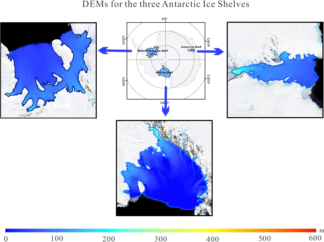
2. Study Areas

3. Data
3.1. Ice, Cloud, and Land Elevation Satellite-2 (ICESat-2) Data
3.2. Operation IceBridge (OIB) Airborne Topographic Mapper (ATM)
3.3. Previously Published Antarctic Digital Elevation Models (DEMs)
3.3.1. Bamber DEM
3.3.2. Helm DEM
3.3.3. TanDEM-X PolarDEM
3.3.4. Slater DEM
3.3.5. Reference Elevation Model of Antarctica (REMA)
4. Methods
4.1. Geostatistical Modeling
4.2. DEM Processing
4.2.1. Data Pre-Processing
4.2.2. Tide Correction
4.2.3. DEM Generation by Tiles
4.2.4. DEM Mosaic
4.2.5. Coastline Mask
5. Result
6. Discussion
6.1. Comparisons with Previous Published DEMs
6.2. Comparison with OIB Airborne Lidar Altimetry Data
7. Conclusions
Supplementary Materials
Author Contributions
Funding
Institutional Review Board Statement
Informed Consent Statement
Data Availability Statement
Acknowledgments
Conflicts of Interest
References
- Rignot, E.; Jacobs, S.; Mouginot, J.; Scheuchl, B. Ice-shelf melting around Antarctica. Science 2013, 341, 266–270. [Google Scholar] [CrossRef] [PubMed] [Green Version]
- Fox, A.J.; Paul, A.; Cooper, R. Measured properties of the Antarctic ice sheet derived from the SCAR Antarctic digital database. Polar Rec. 1994, 30, 201–206. [Google Scholar] [CrossRef]
- Depoorter, M.A.; Bamber, J.L.; Griggs, J.A.; Lenaerts, J.T.M.; Ligtenberg, S.R.M.; van den Broeke, M.R.; Moholdt, G. Calving fluxes and basal melt rates of Antarctic ice shelves. Nature 2013, 502, 89–92. [Google Scholar] [CrossRef]
- Qi, M.; Liu, Y.; Lin, Y.; Hui, F.; Li, T.; Cheng, X. Efficient Location and Extraction of the Iceberg Calved Areas of the Antarctic Ice Shelves. Remote Sens. 2020, 12, 2658. [Google Scholar] [CrossRef]
- Wuite, J.; Nagler, T.; Gourmelen, N.; Escorihuela, M.J.; Hogg, A.E.; Drinkwater, M.R. Sub-Annual Calving Front Migration, Area Change and Calving Rates from Swath Mode CryoSat-2 Altimetry, on Filchner-Ronne Ice Shelf, Antarctica. Remote Sens. 2019, 11, 2761. [Google Scholar] [CrossRef] [Green Version]
- Rignot, E.; Casassa, G.; Gogineni, P.; Krabill, W.; Rivera, A.; Thomas, R. Accelerated ice discharge from the Antarctic Peninsula following the collapse of Larsen B ice shelf. Geophys. Res. Lett. 2004, 31, L18401. [Google Scholar] [CrossRef] [Green Version]
- Stephenson, S.N.; Bindschadler, R.A. Observed velocity fluctuations on a major Antarctic ice stream. Nature 1988, 6184, 695–697. [Google Scholar] [CrossRef]
- Vaughan, D.G.; Arthern, R. CLIMATE CHANGE: Why Is It Hard to Predict the Future of Ice Sheets? Science 2007, 315, 1503–1504. [Google Scholar] [CrossRef] [PubMed] [Green Version]
- Bamber, J.L.; Gomez-Dans, J.L.; Griggs, J.A. A new 1km digital elevation model of the Antarctic derived from combined satellite radar and laser data—Part 1: Data and methods. Cryosphere 2009, 1, 101–111. [Google Scholar] [CrossRef] [Green Version]
- Bamber, J.L.; Griggs, J.A.; Hurkmans, R.T.W.L.; Dowdeswell, J.A.; Gogineni, S.P.; Howat, I.; Mouginot, J.; Paden, J.; Palmer, S.; Rignot, E.; et al. A new bed elevation dataset for Greenland. Cryosphere 2013, 7, 499–510. [Google Scholar] [CrossRef] [Green Version]
- Griggs, J.A.; Bamber, J.L. A new 1km digital elevation model of Antarctica derived from combined radar and laser data—Part 2: Validation and error estimates. Cryosphere 2009, 1, 113–123. [Google Scholar] [CrossRef] [Green Version]
- Wright, A.P.; Siegert, M.J.; Le Brocq, A.M.; Gore, D.B. High sensitivity of subglacial hydrological pathways in Antarctica to small ice-sheet changes. Geophys. Res. Lett. 2008, 35, L17504. [Google Scholar] [CrossRef]
- Wang, Z.; Song, X.; Zhang, B.; Liu, T.; Geng, H. Basal Channel Extraction and Variation Analysis of Nioghalvfjerdsfjorden Ice Shelf in Greenland. Remote Sens. 2020, 12, 1474. [Google Scholar] [CrossRef]
- Xing, Z.; Chi, Z.; Yang, Y.; Chen, S.; Huang, H.; Cheng, X.; Hui, F. Accuracy Evaluation of Four Greenland Digital Elevation Models (DEMs) and Assessment of River Network Extraction. Remote Sens. 2020, 12, 3429. [Google Scholar] [CrossRef]
- Horgan, H.J.; Anandakrishnan, S. Static grounding lines and dynamic ice streams: Evidence from the Siple Coast, West Antarctica. Geophys. Res. Lett. 2006, 33, L18502. [Google Scholar] [CrossRef]
- Paolo, F.S.; Fricker, H.A.; Padman, L. 2015 Volume loss from Antarctic ice shelves is accelerating. Science 2015, 6232, 327–331. [Google Scholar] [CrossRef] [PubMed] [Green Version]
- Smith, B.; Fricker, H.A.; Gardner, A.S.; Medley, B.; Nilsson, J.; Paolo, F.S.; Holschuh, N.; Adusumilli, S.; Brunt, K.; Csatho, B.; et al. Pervasive ice sheet mass loss reflects competing ocean and atmosphere processes. Science 2020, 368, 1239–1242. [Google Scholar] [CrossRef] [PubMed]
- Sutterley, T.C.; Velicogna, I.; Rignot, E.; Mouginot, J.; Flament, T.; van den Broeke, M.R.; van Wessem, J.M.; Reijmer, C.H. Mass loss of the Amundsen Sea Embayment of West Antarctica from four independent techniques. Geophys. Res. Lett. 2015, 41, 8421–8428. [Google Scholar] [CrossRef] [Green Version]
- Young, D.A.; Wright, A.P.; Roberts, J.L.; Warner, R.C.; Young, N.W.; Greenbaum, J.S.; Schroeder, D.M.; Holt, J.W.; Sugden, D.E.; Blankenship, D.D.; et al. A dynamic early East Antarctic Ice Sheet suggested by ice-covered fjord landscapes. Nature 2011, 474, 72–75. [Google Scholar] [CrossRef]
- Yan, S.; Liu, G.; Wang, Y.; Ruan, Z. Accurate Determination of Glacier Surface Velocity Fields with a DEM-Assisted Pixel-Tracking Technique from SAR Imagery. Remote Sens. 2015, 7, 10898–10916. [Google Scholar] [CrossRef] [Green Version]
- Riel, B.; Minchew, B.; Joughin, I. Observing traveling waves in glaciers with remote sensing: New flexible time series methods and application to Sermeq Kujalleq, Greenland. Cryosphere 2021, 15, 407–429. [Google Scholar] [CrossRef]
- Kim, S.; Kim, D. Combined usage of TanDEM-X and CryoSat-2 for generating a high resolution Digital Elevation Model of fast moving ice stream and its application in grounding line estimation. Remote Sens. 2017, 9, 176. [Google Scholar] [CrossRef] [Green Version]
- Bamber, J.L.; Bindschadler, R.A. An improved elevation data set for climate and ice-sheet modeling: Validation with satellite imagery. Ann. Glaciol. 1997, 25, 430–444. [Google Scholar] [CrossRef] [Green Version]
- Helm, V.; Humbert, A.; Miller, H. Elevation and elevation change of Greenland and Antarctica derived from CryoSat-2. Cryosphere 2014, 8, 1539–1559. [Google Scholar] [CrossRef] [Green Version]
- Li, F.; Xiao, F.; Zhang, S.K.; E, D.C.; Cheng, X.; Hao, W.F.; Yuan, L.X.; Zuo, Y.W. DEM development and precision analysis for Antarctic ice sheet using CryoSat-2 altimetry data. Chin. J. Geophys. 2017, 5, 1617–1629. [Google Scholar]
- Slater, T.; Shepherd, A.; McMillan, M.; Muir, A.; Gilbert, L.; Hogg, A.E.; Konrad, H.; Parrinello, T. A new digital elevation model of Antarctica derived from CryoSat-2 altimetry. Cryosphere 2018, 12, 1551–1562. [Google Scholar] [CrossRef] [Green Version]
- DiMarzio, J.; Brenner, A.; Schutz, R.C.; Shuman, A.; Zwally, H.J. GLAS/ICESat 500 m Laser Altimetry Digital Elevation Model of Antarctica; Version 1; NASA National Snow and Ice Data Center Distributed Active Archive Center: Boulder, CO, USA, 2007.
- Rizzoli, P.; Martone, M.; Gonzalez, C.; Wecklich, C.; Borla Tridon, D.; Bräutigam, B.; Bachmann, M.; Schulze, D.; Fritz, T.; Huber, M.; et al. Generation and performance assessment of the global TanDEM-X digital elevation model. ISPRS J. Photogramm. 2017, 132, 119–139. [Google Scholar] [CrossRef] [Green Version]
- Abdullahi, S.; Wessel, B.; Huber, M.; Wendleder, A.; Roth, A.; Kuenzer, C. Estimating Penetration-Related X-Band InSAR Elevation Bias: A Study over the Greenland Ice Sheet. Remote Sens. 2019, 11, 2903. [Google Scholar] [CrossRef] [Green Version]
- Gardelle, J.; Berthier, E.; Arnaud, Y. Impact of resolution and radar penetration on glacier elevation changes computed from DEM differencing. J. Glaciol. 2012, 58, 419–422. [Google Scholar] [CrossRef] [Green Version]
- Gourmelen, N.; Escorihuela, M.J.; Shepherd, A.; Foresta, L.; Muir, A.; Garcia-Mondéjar, A.; Roca, M.; Baker, S.G.; Drinkwater, M.R. CryoSat-2 swath interferometric altimetry for mapping ice elevation and elevation change. Adv. Space Res. 2018, 62, 1226–1242. [Google Scholar] [CrossRef] [Green Version]
- Wessel, B.; Huber, M.; Wohlfart, C.; Marschalk, U.; Kosmann, D.; Roth, A. Accuracy assessment of the global TanDEM-X Digital Elevation Model with GPS data. ISPRS J. Photogramm. 2018, 139, 171–182. [Google Scholar] [CrossRef]
- Du, Y.N.; Feng, G.C.; Li, Z.W.; Zhu, J.J. Generation of high precision DEM from TerraSAR-X/TanDEM-X. Chin. J. Geophys. 2015, 9, 3089–3102. [Google Scholar]
- Gruber, A.; Wessel, B.; Martone, M.; Roth, A. The TanDEM-X DEM Mosaicking: Fusion of Multiple Acquisitions Using InSAR Quality Parameters. IEEE J. Sel. Top. Appl. Earth Obs. Remote Sens. 2016, 9, 1047–1057. [Google Scholar] [CrossRef]
- Howat, I.M.; Porter, C.; Smith, B.E.; Noh, M.; Morin, P. The Reference Elevation Model of Antarctica. Cryosphere 2019, 13, 665–674. [Google Scholar] [CrossRef] [Green Version]
- Rao, Y.S.; Rao, K.S. Comparison of DEMs derived from INSAR and optical stereo techniques. In Proceedings of the Third ESA International Workshop on ERS SAR Interferometry, Frascati, Italy, 1–5 December 2003; Available online: http://citeseerx.ist.psu.edu/viewdoc/download?doi=10.1.1.212.4788&rep=rep1&type=pdf (accessed on 5 October 2020).
- Markus, T.; Neumann, T.; Martino, A.; Abdalati, W.; Brunt, K.; Csatho, B.; Farrell, S.; Fricker, H.; Gardner, A.; Harding, D.; et al. The Ice, Cloud, and land Elevation Satellite-2 (ICESat-2): Science requirements, concept, and implementation. Remote Sens. Environ. 2017, 190, 260–273. [Google Scholar] [CrossRef]
- Abdalati, W.; Zwally, H.J.; Bindschadler, R.; Csatho, B.; Farrell, S.L.; Fricker, H.A.; Harding, D.; Kwok, R.; Lefsky, M.; Markus, T.; et al. The ICESat-2 Laser Altimetry Mission. Proc. IEEE 2010, 98, 735–751. [Google Scholar] [CrossRef]
- Shen, X.Y.; Ke, C.Q.; Yu, X.N.; Cai, Y.; Fan, Y.B. Evaluation of Ice, Cloud, And Land Elevation Satellite-2 (ICESat-2) land ice surface heights using Airborne Topographic Mapper (ATM) data in Antarctica. Int. J. Remote Sens. 2021, 42, 2556–2573. [Google Scholar] [CrossRef]
- Fricker, H.A.; Hyland, G.; Coleman, R.; Young, N.W. Digital elevation models for the Lambert Glacier–Amery Ice Shelf system, East Antarctica, from ERS-1 satellite radar altimetry. J. Glaciol. 2000, 46, 553–560. [Google Scholar] [CrossRef] [Green Version]
- Griggs, J.A.; Bamber, J.L. Antarctic ice-shelf thickness from satellite radar altimetry. J. Glaciol. 2011, 57, 485–498. [Google Scholar] [CrossRef] [Green Version]
- Nguyen, A.T.; Herring, T.A. Analysis of ICESat data using Kalman filter and kriging to study height changes in East Antarctica. Geophys. Res. Lett. 2005, 32, L23S03. [Google Scholar] [CrossRef] [Green Version]
- Strößenreuther, U.; Horwath, M.; Schröder, L. How Different Analysis and Interpolation Methods Affect the Accuracy of Ice Surface Elevation Changes Inferred from Satellite Altimetry. Math. Geosci. 2020, 52, 499–525. [Google Scholar] [CrossRef] [Green Version]
- Chen, C.; Li, Y.A. Fast Global Interpolation Method for Digital Terrain Model Generation from Large LiDAR-Derived Data. Remote Sens. 2019, 11, 1324. [Google Scholar] [CrossRef] [Green Version]
- Koo, Y.; Xie, H.; Kurtz, N.T.; Ackley, S.F.; Mestas-Nuñez, A.M. Weekly Mapping of Sea Ice Freeboard in the Ross Sea from ICESat-2. Remote Sens. 2021, 13, 3277. [Google Scholar] [CrossRef]
- Li, Y.Z.; McGillicuddy, D.J.; Dinniman, M.S.; Klinck, J.M. Processes influencing formation of low-salinity high-biomass lenses near the edge of the Ross Ice Shelf. J. Mar. Syst. 2017, 166, 108–119. [Google Scholar] [CrossRef] [Green Version]
- Grosfeld, K.; Schröder, M.; Fahrbach, E.; Gerdes, R.; Mackensen, A. How iceberg calving and grounding change the circulation and hydrography in the Filchner Ice Shelf-Ocean System. J. Geophys. Res. Ocean. 2001, 106, 9039–9055. [Google Scholar] [CrossRef] [Green Version]
- Yu, J.; Liu, H.X.; Jezek, K.C.; Warner, R.C.; Wen, J. Analysis of velocity field, mass balance, and basal melt of the Lambert Glacier–Amery Ice Shelf system by incorporating Radarsat SAR interferometry and ICESat laser altimetry measurements. J. Geophys. Res. 2010, 115, B11102. [Google Scholar] [CrossRef] [Green Version]
- Robert, B.; Patricia, V.; Andrew, F.; Adrian, F.; Jerry, M.; Douglas, B.; Sara, J.P.; Brian, G.; David, G. The Landsat Image Mosaic of Antarctica. Remote Sens. Environ. 2008, 112, 4214–4426. [Google Scholar]
- Smith, B.; Fricker, H.A.; Holschuh, N.; Gardnerd, A.S.; Adusumillib, S.; Brunte, K.M.; Csathog, B.; Harbecke, K.; Hutha, A.; Neumanne, T.; et al. Land ice height-retrieval algorithm for NASA’s ICESat-2 photon-counting laser altimeter. Remote Sens. Environ. 2019, 233, 111352. [Google Scholar] [CrossRef] [Green Version]
- Neumann, T.A.; Martino, A.J.; Markus, T.; Bae, S.; Bock, M.R.; Brenner, A.C.; Brunt, K.M.; Cavanaugh, J.; Fernandes, S.T.; Hancock, D.W.; et al. The Ice, Cloud, and Land Elevation Satellite—2 mission: A global geolocated photon product derived from the Advanced Topographic Laser Altimeter System. Remote Sens. Environ. 2019, 233, 111325. [Google Scholar] [CrossRef] [PubMed]
- Brunt, K.M.; Neumann, T.A.; Smith, B.E. Assessment of ICESat-2 Ice Sheet Surface Heights, Based on Comparisons over the Interior of the Antarctic Ice Sheet. Geophys. Res. Lett. 2019, 46, 13072–13078. [Google Scholar] [CrossRef] [Green Version]
- Li, R.X.; Li, H.W.; Hao, T.; Qiao, G.; Cui, H.T.; He, Y.Q.; Hai, G.; Xie, H.; Cheng, Y.; Li, B.F. Assessment of ICESat-2 ice surface elevations over the Chinese Antarctic Research Expedition (CHINARE) route, East Antarctica, based on coordinated multi-sensor observations. Cryosphere 2021, 15, 3083–3099. [Google Scholar] [CrossRef]
- Kurtz, N.T.; Farrell, S.L.; Studinger, M.; Galin, N.; Harbeck, J.P.; Lindsay, R.; Onana, V.D.; Panzer, B.; Sonntag, J.G. Sea ice thickness, freeboard, and snow depth products from Operation IceBridge airborne data. Cryosphere 2013, 7, 1035–1056. [Google Scholar] [CrossRef] [Green Version]
- Martin, C.F.; Krabill, W.B.; Manizade, S.S.; Russell, R.L.; Sonntag, J.G.; Swift, R.N.; Yungel, J.K. Airborne Topographic Mapper Calibration Procedures and Accuracy Assessment; NASA: Washington, DC, USA, 2012.
- Studinger, M. IceBridge ATM L2 Icessn Elevation, Slope, and Roughness; Version 2; NASA National Snow and Ice Data Center Distributed Active Archive Center: Boulder, CO, USA, 2014.
- Cook, A.J.; Murray, T.; Luckman, A.; Vaughan, D.G.; Barrand, N.E. A new 100-m Digital Elevation Model of the Antarctic Peninsula derived from ASTER Global DEM: Methods and accuracy assessment. Earth Syst. Sci. Data 2012, 4, 129–142. [Google Scholar] [CrossRef] [Green Version]
- Oliver, M.A.; Webster, R. Kriging: A method of interpolation for geographical information systems. Int. J. Geogr. Inf. Syst. 1990, 4, 313–332. [Google Scholar] [CrossRef]
- Oliver, M.A.; Webster, R. Basic Steps in Geostatistics: The Variogram and Kriging; Springer International Press: Cham, Switzerland, 2015; p. 112. [Google Scholar]
- Bamber, J.; Gomez-Dans, J.L. The accuracy of digital elevation models of the Antarctic continent. Earth Planet. Sci. Lett. 2005, 237, 516–523. [Google Scholar] [CrossRef]
- Ray, R.D. A Global Ocean Tide Model from TOPEX/POSEIDON Altimetry: GOT99. 2. NASA Technical Memorandum 209478; Goddard Space Flight Center: Washington, DC, USA, 1999.
- Neumann, T.A.; Brenner, A.; Hancock, D.; Robbins, J.; Saba, J.; Harbeck, K.; Gibbons, A.; Lee, J.; Luthcke, S.B.; Rebold, T. Algorithm Theoretical Basis Document (ATBD) for Global Geolocated Photons ATL03, Version 3, Release Date 1 April 2020. 2020. Available online: https://nsidc.org/sites/nsidc.org/files/technical-references/ICESat2_ATL03_ATBD_r003.pdf (accessed on 5 October 2020).
- Gerrish, L.; Fretwell, P.; Cooper, P. High Resolution Vector Polylines of the Antarctic Coastline; Version 7.2; UK Polar Data Centre, Natural Environment Research Council and UK Research and Innovation: Cambridge, UK, 2020. [Google Scholar]


| Bamber DEM | Helm DEM | TanDEM-X PolarDEM | Slater DEM | REMA | |
|---|---|---|---|---|---|
| Published time | 2009 | 2014 | 2017 | 2018 | 2018 |
| Source data | ERS-1 and ICESat | CryoSat-2 | TerraSAR-X and TanDEM-X | CryoSat-2 | WorldView-1/2/3 and GeoEye-1 |
| Coverage | Ice sheet | Pan-Antarctica | Global | Pan-Antarctica | Pan-Antarctica |
| Spatial resolution | 1 km | 1 km | 12 m, 30 m, 90 m | 1 km | 8 m, 100 m, 200 m, 1 km |
| Time span of applied source data | March 1994–May 1995, February 2003–March 2008 | January 2012– January 2013 | December 2010–January 2015 | July 2010–July 2016 | 2010–2018 |
| RIS | FRIS | AIS | ||||
|---|---|---|---|---|---|---|
| Variogram Model | Linear | Spherical | Linear | Spherical | Linear | Spherical |
| Mean/m | 0.011 | 0.032 | −0.016 | 0.018 | −0.006 | −0.004 |
| Std/m | 2.979 | 2.769 | 3.376 | 2.215 | 2.287 | 1.394 |
| Mean/m | Std/m | Maximum/m | Minimum/m | |
|---|---|---|---|---|
| RIS DEM | 9.772 | 24.087 | 1280.716 | −5.441 |
| FRIS DEM | 73.213 | 31.082 | 925.373 | −21.361 |
| AIS DEM | 97.192 | 38.412 | 1176.542 | −15.466 |
| ICESat-2 RIS DEM vs. | Mean/m | Std/m |
|---|---|---|
| REMA | 0.715 | 2.493 |
| TanDEM-X PolarDEM | 4.940 | 2.767 |
| Slater DEM | 0.408 | 2.290 |
| Helm DEM | 0.536 | 2.824 |
| Bamber DEM | −0.022 | 2.674 |
| ICESat-2 FRIS DEM vs. | Mean/m | Std/m |
|---|---|---|
| REMA | −0.228 | 2.955 |
| TanDEM-X PolarDEM | 1.738 | 3.476 |
| Slater DEM | 0.674 | 2.640 |
| Helm DEM | 0.956 | 4.604 |
| Bamber DEM | 0.510 | 3.012 |
| ICESat-2 AIS DEM vs. | Mean/m | Std/m |
|---|---|---|
| REMA | −0.116 | 5.294 |
| TanDEM-X PolarDEM | 1.302 | 5.381 |
| Slater DEM | 0.226 | 4.832 |
| Helm DEM | −0.891 | 5.044 |
| Bamber DEM | 0.002 | 5.248 |
| OIB Elevations vs. | Mean/m | Std/m |
|---|---|---|
| ICESat-2 RIS DEM | −0.016 | 0.918 |
| TanDEM-X PolarDEM | 5.254 | 2.203 |
| REMA | 0.828 | 1.805 |
| Slater DEM | 0.485 | 1.853 |
| Helm DEM | 0.804 | 1.733 |
| Bamber DEM | 0.187 | 1.934 |
| OIB Elevations vs. | Mean/m | Std/m |
|---|---|---|
| ICESat-2 FRIS DEM | −0.533 | 0.718 |
| TanDEM-X PolarDEM | 1.727 | 1.924 |
| REMA | 0.572 | 1.096 |
| Slater DEM | −0.097 | 0.947 |
| Helm DEM | 0.077 | 1.173 |
| Bamber DEM | −0.557 | 1.382 |
Publisher’s Note: MDPI stays neutral with regard to jurisdictional claims in published maps and institutional affiliations. |
© 2021 by the authors. Licensee MDPI, Basel, Switzerland. This article is an open access article distributed under the terms and conditions of the Creative Commons Attribution (CC BY) license (https://creativecommons.org/licenses/by/4.0/).
Share and Cite
Geng, T.; Zhang, S.; Xiao, F.; Li, J.; Xuan, Y.; Li, X.; Li, F. DEM Generation with ICESat-2 Altimetry Data for the Three Antarctic Ice Shelves: Ross, Filchner–Ronne and Amery. Remote Sens. 2021, 13, 5137. https://0-doi-org.brum.beds.ac.uk/10.3390/rs13245137
Geng T, Zhang S, Xiao F, Li J, Xuan Y, Li X, Li F. DEM Generation with ICESat-2 Altimetry Data for the Three Antarctic Ice Shelves: Ross, Filchner–Ronne and Amery. Remote Sensing. 2021; 13(24):5137. https://0-doi-org.brum.beds.ac.uk/10.3390/rs13245137
Chicago/Turabian StyleGeng, Tong, Shengkai Zhang, Feng Xiao, Jiaxing Li, Yue Xuan, Xiao Li, and Fei Li. 2021. "DEM Generation with ICESat-2 Altimetry Data for the Three Antarctic Ice Shelves: Ross, Filchner–Ronne and Amery" Remote Sensing 13, no. 24: 5137. https://0-doi-org.brum.beds.ac.uk/10.3390/rs13245137