
Statistical Analysis for Tidal Flat Classification and Topography Using Multitemporal SAR Backscattering Coefficients


Abstract
:1. Introduction
2. Materials and Methods
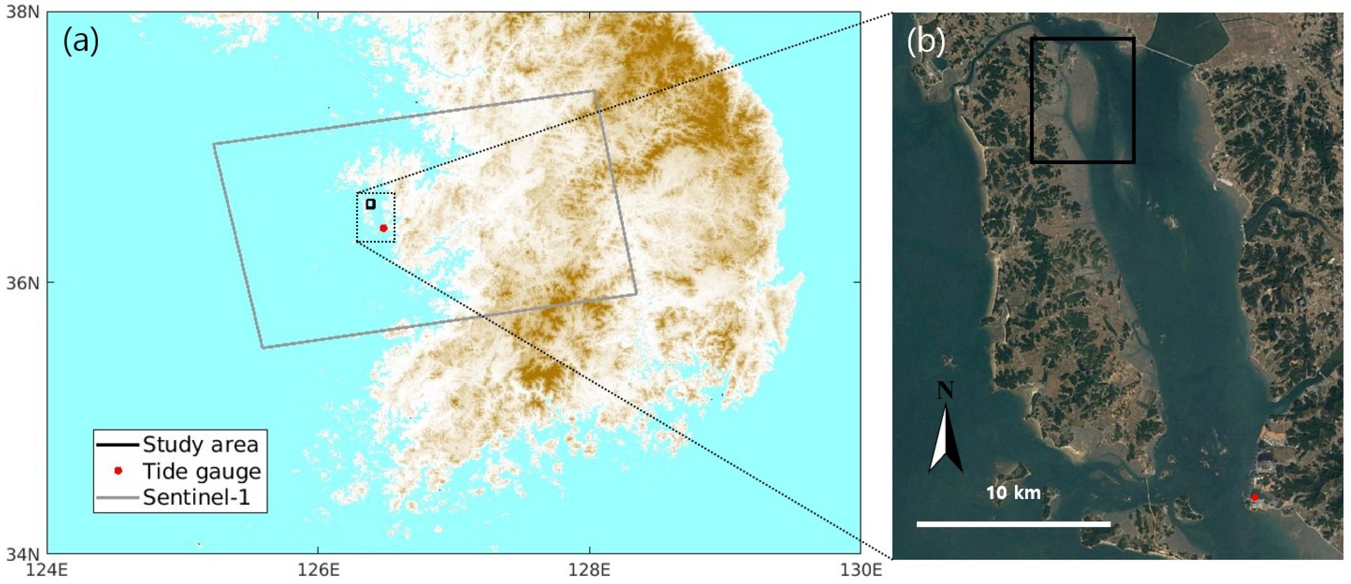
2.1. Study Area
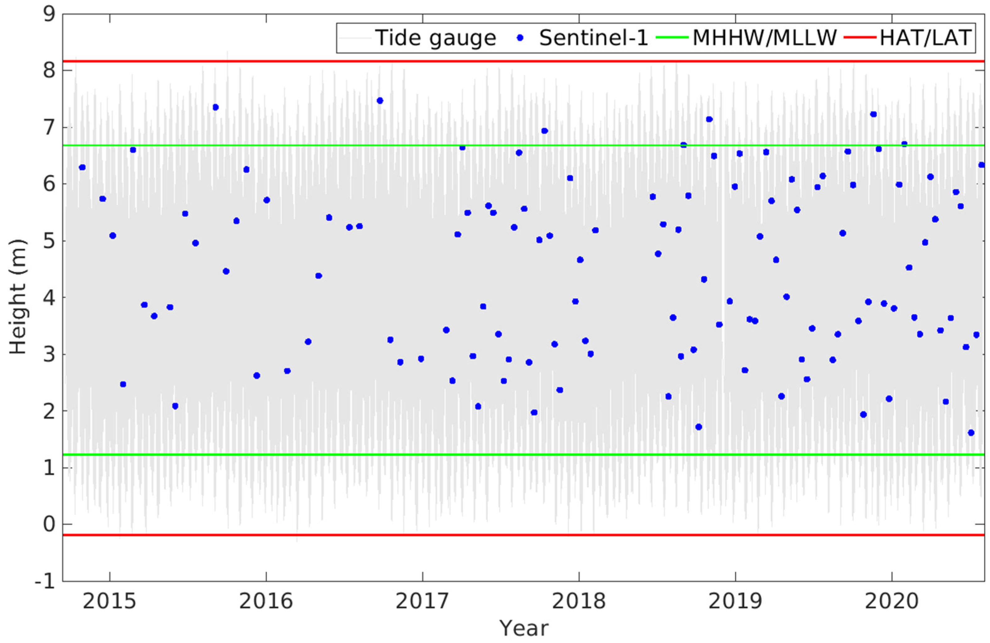
2.2. Tide
2.3. SAR Image Processing
2.4. Statistical Analysis
2.4.1. JNB Optimization
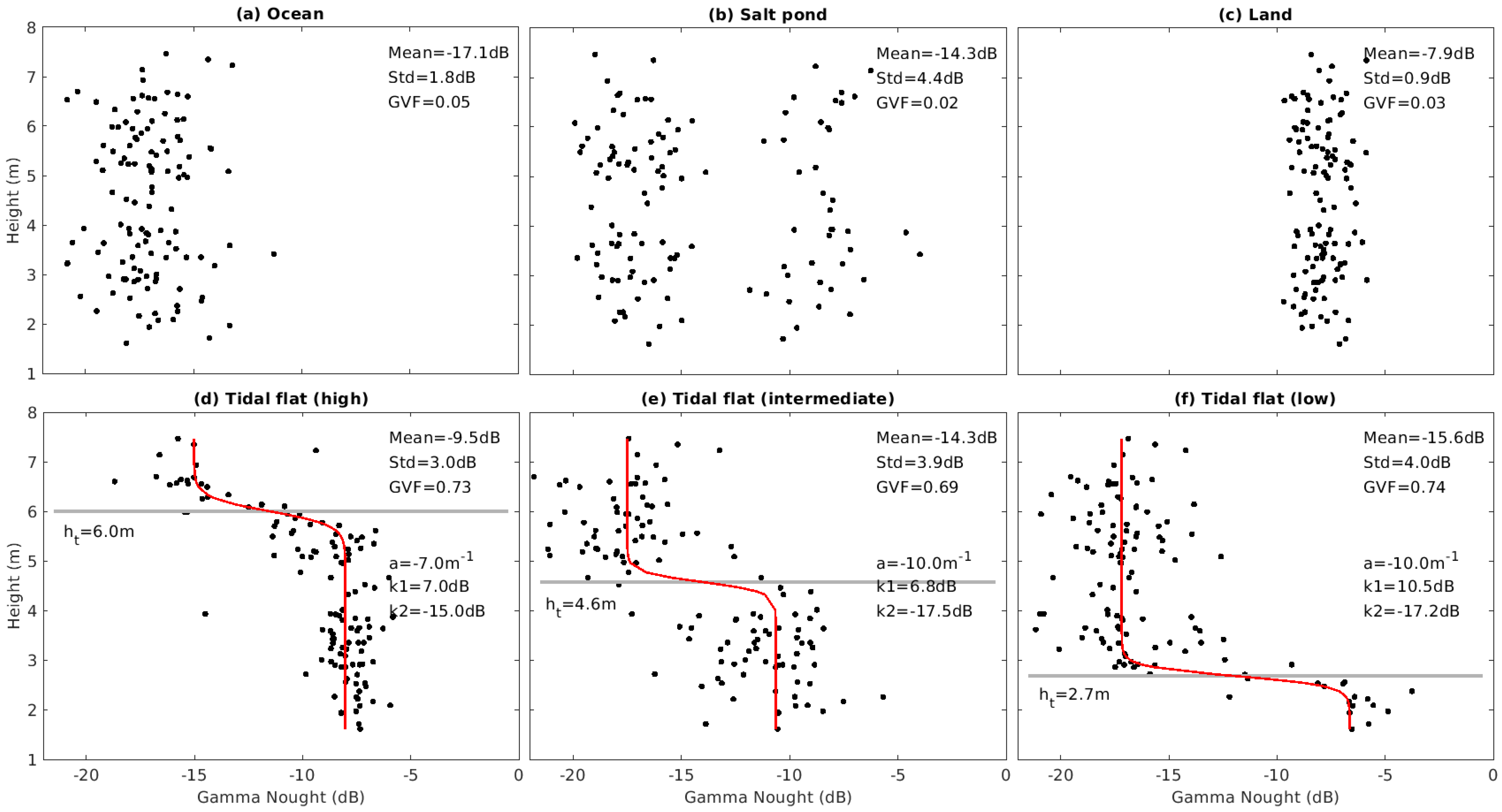
2.4.2. Logistic Function
2.5. DEM Evaluation
3. Results and Discussion
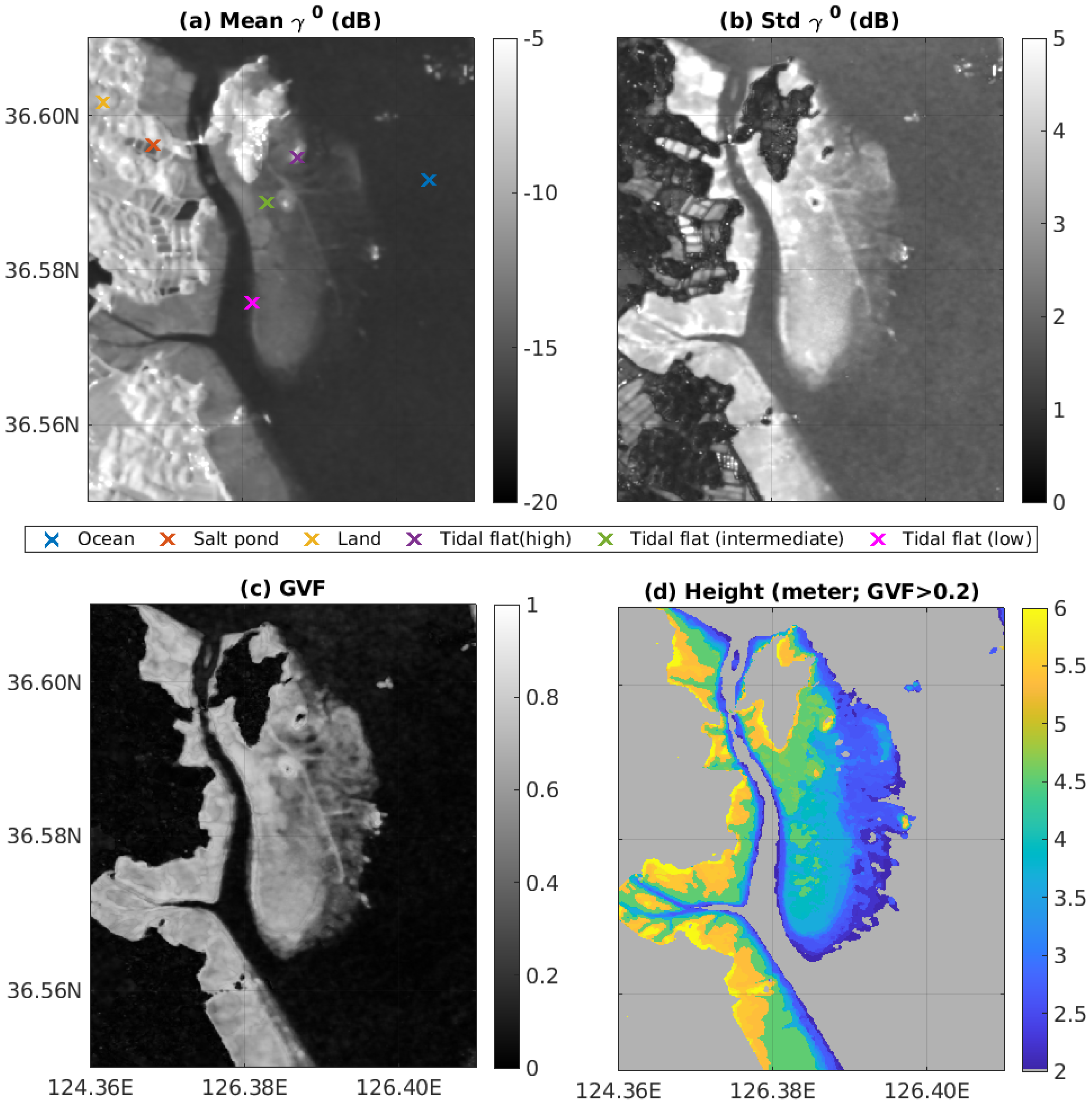
3.1. Statistical Analysis
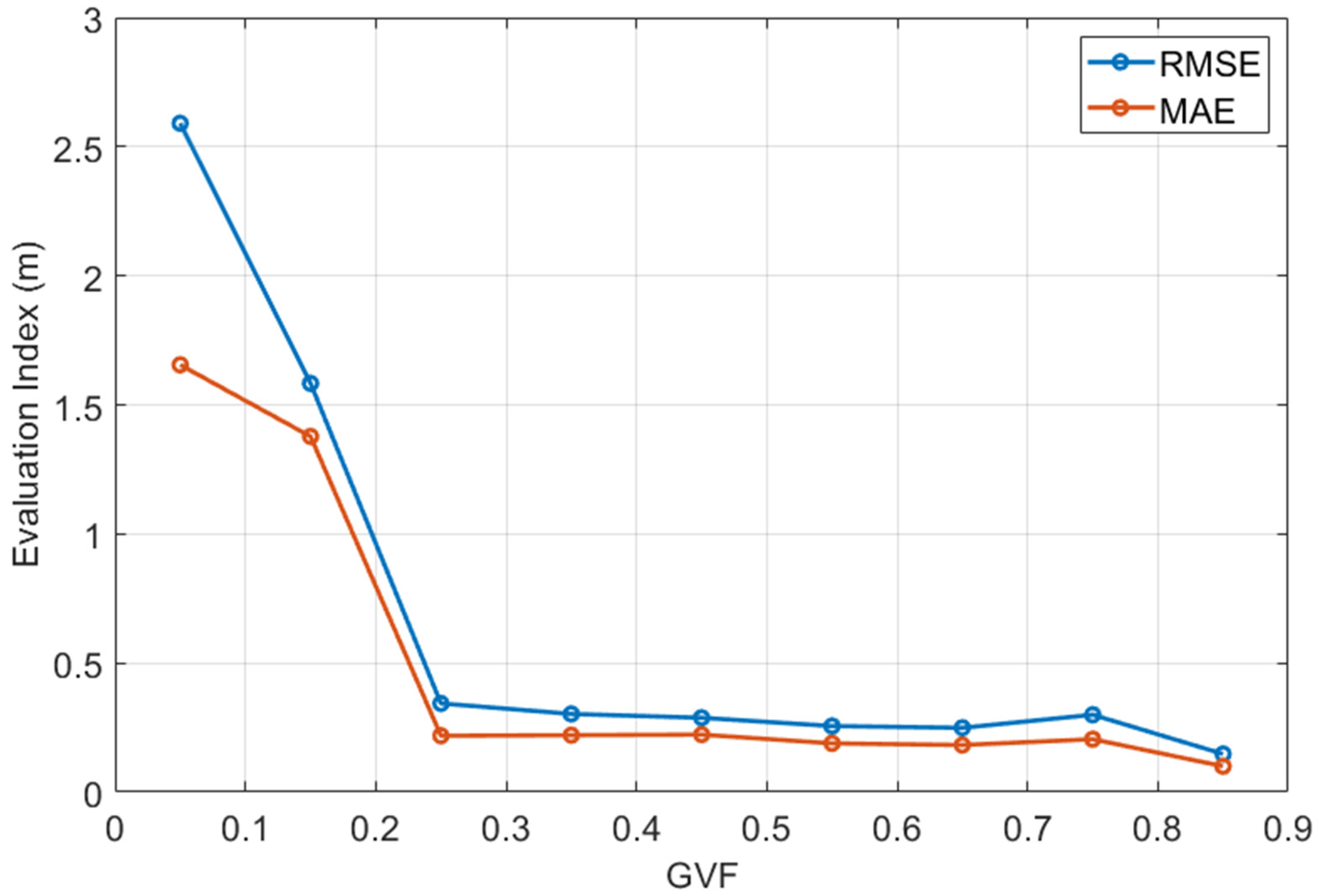
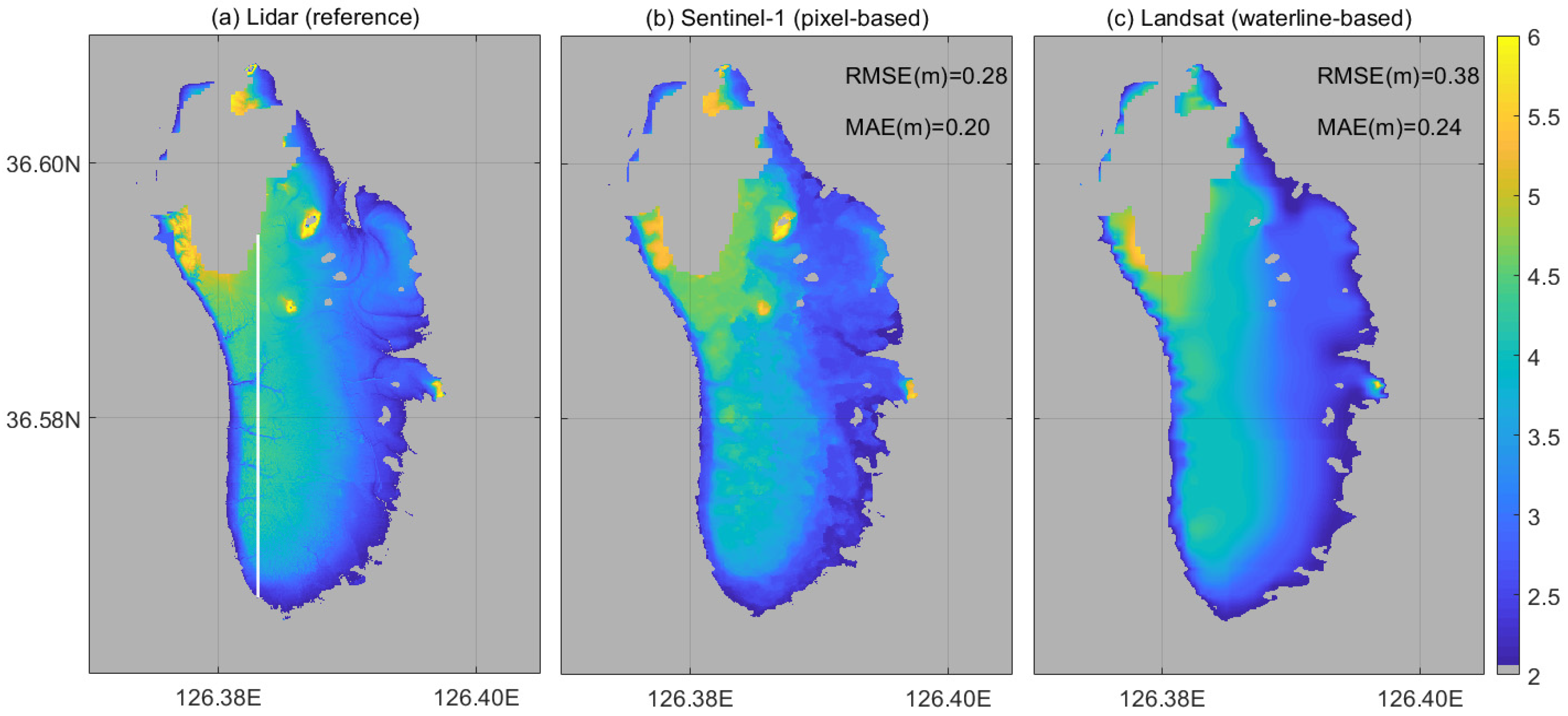
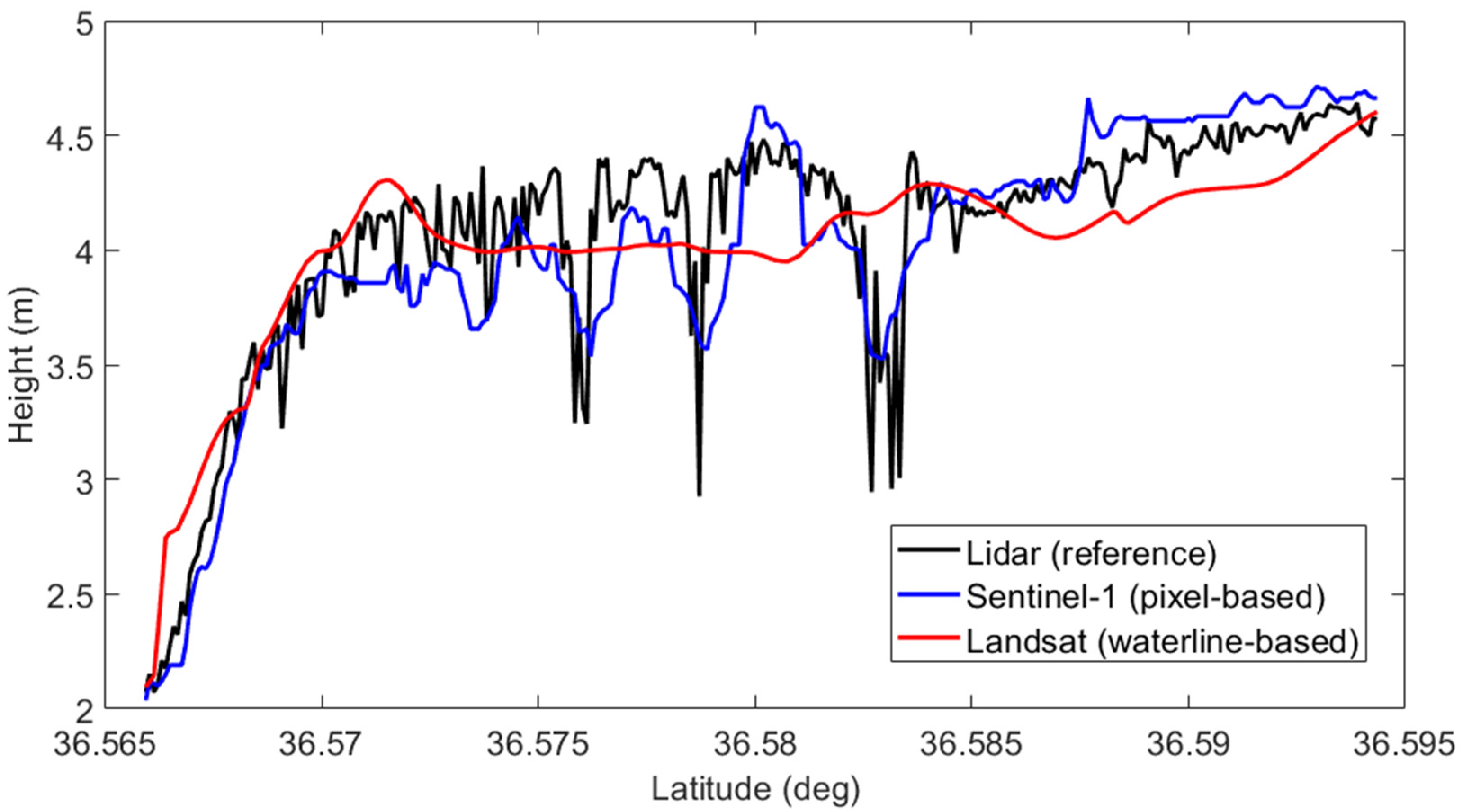
3.2. DEM Evaluation
4. Conclusions
Author Contributions
Funding
Conflicts of Interest
References
- Murray, N.; Phinn, S.R.; DeWitt, M.; Ferrari, R.; Johnston, R.; Lyons, M.B.; Clinton, N.; Thau, D.; Fuller, R.A. The global distribution and trajectory of tidal flats. Nature 2019, 565, 222–225. [Google Scholar] [CrossRef] [PubMed]
- Salameh, E.; Frappart, F.; Turki, I.; Laignel, B. Intertidal topography mapping using the waterline method from Sentinel-1 & -2 images: The examples of Arcachon and Veys Bays in France. ISPRS J. Photogramm. Remote Sens. 2020, 163, 98–120. [Google Scholar] [CrossRef]
- Allen, J.R.L.; Pye, K. (Eds.) Coastal saltmarshes: Their nature and significance. In Saltmarshes: Morphodynamics, Conservation and Engineering Significance; Cambridge University Press: Cambridge, UK, 1992; pp. 1–18. [Google Scholar]
- You, S.J.; Kim, J.G. Evaluation on the purification capacity of pollutants in the tidal flat. J. Korean Fish. Soc. 1999, 32, 409–415. [Google Scholar]
- Woo, H.J.; Choi, J.U.; Ryu, J.H.; Choi, S.H.; Kim, S.R. Sedimentary environments in the Hwangdo tidal flat, Cheonsu Bay. J. Wetlands Soc. 2005, 7, 53–67. [Google Scholar]
- MLTM. The Basic Survey of Coastal Wetland in 2008; Ministry of Land, Transport and Marine Affairs: Sejong, Korea, 2010; 383p. (In Korean) [Google Scholar]
- Lee, Y.-K.; Ryu, J.-H.; Choi, J.-K.; Lee, S.; Woo, H.-J. Satellite-based observations of unexpected coastal changes due to the Saemangeum Dyke construction, Korea. Mar. Pollut. Bull. 2015, 97, 150–159. [Google Scholar] [CrossRef] [PubMed]
- Murray, N.J.; Phinn, S.R.; Clemens, R.S.; Roelfsema, C.M.; Fuller, R.A. Continental Scale Mapping of Tidal Flats across East Asia Using the Landsat Archive. Remote Sens. 2012, 4, 3417–3426. [Google Scholar] [CrossRef] [Green Version]
- Choi, J.-K.; Ryu, J.-H.; Lee, Y.-K.; Yoo, H.-R.; Woo, H.J.; Kim, C.H. Quantitative estimation of intertidal sediment characteristics using remote sensing and GIS. Estuar. Coast. Shelf Sci. 2010, 88, 125–134. [Google Scholar] [CrossRef]
- Long, N.; Millescamps, B.; Guillot, B.; Pouget, F.; Bertin, X. Monitoring the Topography of a Dynamic Tidal Inlet Using UAV Imagery. Remote Sens. 2016, 8, 387. [Google Scholar] [CrossRef] [Green Version]
- Brunetta, R.; Duo, E.; Ciavola, P. Evaluating Short-Term Tidal Flat Evolution Through UAV Surveys: A Case Study in the Po Delta (Italy). Remote Sens. 2021, 13, 2322. [Google Scholar] [CrossRef]
- Ryu, J.-H.; Kim, C.-H.; Lee, Y.-K.; Won, J.-S.; Chun, S.-S.; Lee, S. Detecting the intertidal morphologic change using satellite data. Estuar. Coast. Shelf Sci. 2008, 78, 623–632. [Google Scholar] [CrossRef]
- Sagar, S.; Roberts, D.; Bala, B.; Lymburner, L. Extracting the intertidal extent and topography of the Australian coastline from a 28 year time series of Landsat observations. Remote Sens. Environ. 2017, 195, 153–169. [Google Scholar] [CrossRef]
- Al Fugura, A.; Billa, L.; Pradhan, B. Semi-automated procedures for shoreline extraction using single RADARSAT-1 SAR image. Estuar. Coast. Shelf Sci. 2011, 95, 395–400. [Google Scholar] [CrossRef]
- Ryu, J.-H.; Won, J.-S.; Min, K.D. Waterline extraction from Landsat TM data in a tidal flat: A case study in Gomso Bay, Korea. Remote Sens. Environ. 2002, 83, 442–456. [Google Scholar] [CrossRef]
- Zhang, M.; Li, Z.; Tian, B.; Zhou, J.; Tang, P. The backscattering characteristics of wetland vegetation and water-level changes detection using multi-mode SAR: A case study. Int. J. Appl. Earth Obs. Geoinf. 2016, 45, 1–13. [Google Scholar] [CrossRef]
- Salameh, E.; Frappart, F.; Almar, R.; Baptista, P.; Heygster, G.; Lubac, B.; Raucoules, D.; Almeida, L.P.; Bergsma, E.W.J.; Capo, S.; et al. Monitoring Beach Topography and Nearshore Bathymetry Using Spaceborne Remote Sensing: A Review. Remote Sens. 2019, 11, 2212. [Google Scholar] [CrossRef] [Green Version]
- Xu, Z.; Kim, D.-J.; Kim, S.H.; Cho, Y.-K.; Lee, S.-G. Estimation of seasonal topographic variation in tidal flats using waterline method: A case study in Gomso and Hampyeong Bay, South Korea. Estuar. Coast. Shelf Sci. 2016, 183, 213–220. [Google Scholar] [CrossRef] [Green Version]
- Heygster, G.; Dannenberg, J.; Notholt, J. Topographic mapping of the german tidal flats analyzing SAR images with the waterline method. IEEE Trans. Geosci. Remote Sens. 2010, 48, 1019–1030. [Google Scholar] [CrossRef]
- Liu, Y.; Li, M.; Zhou, M.; Yang, K.; Mao, L. Quantitative Analysis of the Waterline Method for Topographical Mapping of Tidal Flats: A Case Study in the Dongsha Sandbank, China. Remote Sens. 2013, 5, 6138–6158. [Google Scholar] [CrossRef] [Green Version]
- Wei, X.; Zheng, W.; Xi, C.; Shang, S. Shoreline Extraction in SAR Image Based on Advanced Geometric Active Contour Model. Remote Sens. 2021, 13, 642. [Google Scholar] [CrossRef]
- Ryu, J.H.; Cho, W.J.; Won, J.S.; Lee, I.T.; Chun, S.S.; Suh, A.S.; Kim, K.L. Intertidal DEM generation using waterline extracted from remotely sensed data. J. Korean Soc. Remote Sens. 2000, 16, 221–233. [Google Scholar]
- Kim, S.J.; Bang, R.S.; Kwon, H.J. Estimation of areal change in Hwa-ong flat due to Sea Dike Construction Project using multi-temporal Landsat TM images. KCID J. 2003, 10, 73–79. [Google Scholar]
- Kim, K.-L.; Kim, B.-J.; Lee, Y.-K.; Ryu, J.-H. Generation of a Large-Scale Surface Sediment Classification Map using Unmanned Aerial Vehicle (UAV) Data: A Case Study at the Hwang-do Tidal Flat, Korea. Remote Sens. 2019, 11, 229. [Google Scholar] [CrossRef] [Green Version]
- Choi, J.-K.; Oh, H.-J.; Koo, B.J.; Ryu, J.-H.; Lee, S. Spatial polychaeta habitat potential mapping using probabilistic models. Estuar. Coast. Shelf Sci. 2011, 93, 98–105. [Google Scholar] [CrossRef]
- So, J.G.; Jeong, G.T.; Chae, J.W. Numerical modeling of changes in tides and tidal currents caused by embankment at chonsu bay. J. Korean Soc. Coast. Ocean. Eng. 1998, 10, 151–164. (In Korean) [Google Scholar]
- Torres, R.; Snoeij, P.; Geudtner, D.; Bibby, D.; Davidson, M.; Attema, E.; Potin, P.; Rommen, B.; Floury, N.; Brown, M.; et al. GMES Sentinel-1 mission. Remote Sens. Environ. 2012, 120, 9–24. [Google Scholar] [CrossRef]
- Jenks, G.F. The data model concept in statistical mapping. Int. Yearb. Cartogr. 1967, 7, 186–190. [Google Scholar]
- Catalao, J.; Nico, G. Multitemporal Backscattering Logistic Analysis for Intertidal Bathymetry. IEEE Trans. Geosci. Remote Sens. 2017, 55, 1066–1073. [Google Scholar] [CrossRef]
- Lee, H.; Chae, H.; Cho, S.-J. Radar backscattering of intertidal mudflats observed by radarsat-1 SAR images and ground-based scatterometer experiments. IEEE Trans. Geosci. Remote Sens. 2011, 49, 1701–1711. [Google Scholar] [CrossRef]
- Ehler, C.; Zaucha, J.; Gee, K. Maritime/marine spatial planning at the interface of research and practice. In Maritime Spatial Planning: Past, Present, Future; Zaucha, J., Gee, K., Eds.; Palgrave Macmillan: Cham, Switzerland, 2019. [Google Scholar] [CrossRef] [Green Version]


Publisher’s Note: MDPI stays neutral with regard to jurisdictional claims in published maps and institutional affiliations. |
© 2021 by the authors. Licensee MDPI, Basel, Switzerland. This article is an open access article distributed under the terms and conditions of the Creative Commons Attribution (CC BY) license (https://creativecommons.org/licenses/by/4.0/).
Share and Cite
Kim, K.; Jung, H.C.; Choi, J.-K.; Ryu, J.-H. Statistical Analysis for Tidal Flat Classification and Topography Using Multitemporal SAR Backscattering Coefficients. Remote Sens. 2021, 13, 5169. https://0-doi-org.brum.beds.ac.uk/10.3390/rs13245169
Kim K, Jung HC, Choi J-K, Ryu J-H. Statistical Analysis for Tidal Flat Classification and Topography Using Multitemporal SAR Backscattering Coefficients. Remote Sensing. 2021; 13(24):5169. https://0-doi-org.brum.beds.ac.uk/10.3390/rs13245169
Chicago/Turabian StyleKim, Keunyong, Hahn Chul Jung, Jong-Kuk Choi, and Joo-Hyung Ryu. 2021. "Statistical Analysis for Tidal Flat Classification and Topography Using Multitemporal SAR Backscattering Coefficients" Remote Sensing 13, no. 24: 5169. https://0-doi-org.brum.beds.ac.uk/10.3390/rs13245169