1. Introduction
The Container Terminal Altenwerder (CTA) is a highly automated terminal located in Hamburg and contributes heavily to transport through the shipping industry. The containers are loaded from the ship to an automated guided vehicle (AGV) which carries them to the storage block for temporary storage. There the rail mounted gantry cranes (RMGC) pick up the container and either put them in the block for storage or bring them to the land side for further transfer. The RMGC is subject to great demands in terms of unchanged position and exact tracking. However, the geomorphological condition of the ground in the port continually leads to significant subsidence and track changes in the rail systems, which therefore must be regularly checked and maintained. Traditional semi-automatic methods for surveying the exact rail location are very complex and costly. They are associated with a residual risk in terms of occupational safety and lead to container storage areas being closed for a day, which can lead to corresponding operational and capacity losses.
In this paper, we present the concept, implementation, and evaluation for automatic delineation of the crane tracks at the Container Terminal in Altenwerder based on UAV-based photogrammetry. We present, besides others, the selection of suitable UAV and camera components, the design and realization of a very high-quality geodetic control network, the development of a suitable ground marking concept, the systematic planning and execution of the flight and photogrammetric bundle block adjustment and finally an automatic delineation of the rails from derived height models and ortho images. The work was carried out during the research project AeroInspekt, funded by the German Ministry of Transportation and Digital Infrastructure (BMVI).
The discussion focuses on the state of our system during the third field test campaign held in June 2020 (CTA3). In CTA3, different improvements have been carried out in comparison to the first campaign CTA1 [
1]. For instance, a new combination of prism and coded target was employed to reduce the survey time for the ground control points (GCPs) and increase the accuracy. In addition, the mission planning software for the UAV during the CTA1 was the first prototype and hence had only limited path planning capabilities without the functionality of dynamic planning. The updated software used in CTA3 now can integrate multiple sources of crane occlusion detection and is modular in nature for the possibility of easy extension. In the following, we will first review related work and then discuss the selection of the flight and camera system, with an additional question concerning the laboratory calibration of the camera parameters, image quality, and spatial resolution. Subsequently, details of the network measurement and the improvements that have been carried out, which is necessary for the positioning of the ground control points, are explained. The fifth chapter is dedicated to flight planning and data acquisition. The sixth chapter details the methodology for the automatic measurement of the track position in the elevation model. Chapter seven finally deals with the results obtained, before the paper is concluded.
2. Related Work
Different systems for railway detection have been used and tested in the past. Most of them are based on traditional surveying or 3D Terrestrial Laser Scanning (TLS) systems. Kregar, et al. [
2] used terrestrial laser scanning (TLS) for measuring the geometry of the crane rails such as the positional and altitude deviations, the span, and height differences between the rails. The results also were compared with the one obtained from the classical polar method, which is considered as a reference measurement. The results showed that both methods are comparable with 0.2 mm in favor of the classical method.
Dennig, et al. [
3] developed an advanced rail tracking inspection system (ARTIS) to measure the 3D position of crane rails, the cross-section, joints, and the fastening. The system is complex and consists of different sensors that need a calibration process to meet the required accuracy.
Xiong, et al. [
4] have developed a 3D laser profiling system for rail surface defect detection. The system integrated different components to capture the rail surface profile data. The system can detect different rail surface defects such as abrasion, corrugation, scratch, corrosion, and peeling with millimeter precision. The results showed that the system can detect defects with lengths larger than 2 mm, widths larger than 0.6 mm, and depths larger than 0.5 mm. However, the system must be calibrated before performing the measurements. In addition, the system is very complex and needs special preparation on the railway directly and that is time consuming as well.
A drone platform called Vogel R3D has been developed to facilitate the 3D measurements of railway infrastructure to sub-5 mm accuracy [
5]. A Phase One industrial 100-megapixel camera was used to capture overlapping high-resolution images and processed using photogrammetry. After processing, the railway survey and topographical survey were conducted using high-resolution orthophoto and highly detailed colored point clouds.
3. System Selection and Camera Calibration
According to the German VDI 3576 guideline or the specification of the cranes, a tolerance of +/− 10 mm applies to the track location and the height tolerance is +/− 100 mm. Kuhlmann et al. [
6] describe the conversion from tolerance values to standard deviation σ as σ = T/4, with T: tolerance applies for a probability of error of 5% for the measuring accuracy to be maintained. Hence, for this project, a measuring accuracy of σxy = 2.5 mm is considered for the location and σz = 25 mm for the height accuracy.
From these data and the requirements resulting from the tolerance, it is clear that a 3D control point field with very high accuracy requirements must be realized for a thorough realization and verification. This aspect is addressed in
Section 4. To meet the accuracy requirement of σxy = 2.5 mm, a ground sampling distance of 1 mm was targeted for the Camera sensor selection. A suitable launch system needs to be able to carry this camera with easy interface conditions. The following section describes the selection of the camera and the launch system in more detail.
3.1. Launch System and Camera
To achieve the required accuracy and avoid field problems, special features and requirements must be considered. These requirements were already explained in the previous paper [
1] but they can be summarized as follows:
Keeping a safe flight distance to the crane in operation. The maximum height of the cranes is 30 m and hence keeping a 5 m margin over this 35 m altitude was fixed for the UAV flight.
The ground sample distance should be small enough to meet the limiting accuracy requirement of σxy = 2.5 mm. In addition, the detailed delineation of rails would also depend on a dense-matching-based surface model, where the edges need to be clearly separated. In order to guarantee that edges are well located, we estimated that the ground sampling distance (GSD) must be better than σxy by a factor of 2 to 3. Besides the required geometric accuracy, the resolution at the object is an important factor in order to be able to delineate the rail outline as accurately as possible. Therefore, considering all those aspects, a GSD of 1 mm was aimed for, also based on the available camera–lens combination in the market.
The pixel pitch of the camera sensor should be big enough to ensure a good signal-to-noise ratio and to be able to achieve short exposure times.
The UAV system should guarantee to carry a relatively heavy payload for a long enough flight. Additionally, positioning via Real-Time Kinematic (RTK) based on global navigation satellite systems is highly recommended for precise navigation and geo-referencing of the captured images.
To meet the above conflicting requirements and after market research, the following system was selected for the project:
- -
Camera sensor: PhaseOne iXM-100 with a resolution of 11.664 × 8.750, sensor size of 43.9 mm × 32.9 mm (medium format), pixel size of D = 3.8 µm and a mass of 630 g.
- -
Camera Lens: PhaseOne RSM 150 mm: focal length f = 150 mm (diagonal aperture angle at the selected sensor: 19°), mass: 750 g.
- -
UAV: DJI Matrice M600 Pro with differential RTK system for navigation and Ronin MX Gimbal (mass: 2150 g) for the camera stabilization, flight time nominal with full battery and the payload of approx. 3.6 kg: 20 min.
Based on this configuration, the theoretical characteristics at a flight altitude of 35 m are (1) image scale factor: m = 235, and (2) ground sampling distance (GSD). In addition, the point measurement accuracy can be defined as (a) image coordinates: , and (b) object coordinates:
The height measurement accuracy can be estimated by the height–base ratio. In the best case, the base is half the image width with a transversely mounted camera, i.e., about 4.5 m. This means that the height accuracy theoretically deteriorates by factor H/W = 35/4.5 ≈ 7 compared to the XY accuracy. However, since there is a high overlap and thus redundancy, this factor can be corrected accordingly [
7] for multi-image photogrammetry using √k
3, where k represents the number of images in which a point is observed.
3.2. Camera Calibration
As explained in [
1], in this project we are facing the difficulty that the area which is surveyed by the chosen system does not show much height variations, hence a simultaneous calibration of the internal camera parameters, especially of the focal length, is not favorable. In addition, the optics of the chosen system can only be focused to infinity from an object distance of 750 m, which is attributed to the relatively long focal length. Up to this range, the focal plane corresponding to the distance is adjusted by a motor. According to the manufacturer’s specifications, the focal plane can be approached with an accuracy of approx. 6 micrometers, i.e., 1.5 pixels. As described in [
1], the camera was pre-calibrated in the lab of DLR (Institute of Optical Sensor Systems) applying the diffractive optical elements (DOE) method [
8]. The results of [
1] suggest that the final results of the bundle block adjustment do not differ significantly between different camera calibration scenarios.
3.3. Image Quality and Spatial Resolution
The tool chain deriving 3D models from aerial imagery benefits greatly from better image quality especially from better spatial resolution [
8]. It is therefore advantageous to have knowledge of the spatial resolution of a specific sensor–lens combination in order to quantify later uncertainties (e.g., of bundle block adjustment or dense image matching).
Image quality of a sensor system is affected by multiple factors and directly influences perceptible detail in aerial images. Light rays being reflected by an object and detected by a camera sensor partially traverse the atmosphere and lose some of their energy due to diffusion and absorption. In drone applications, this part could be considered very small and will not be discussed further here.
Next, the light passes a (complex) lens system where an aperture is integrated and limits the effective solid angles for every ray. Consequently, the lens-aperture directly affects the amount of light which in turn determines the number of photons that reach the sensor plane and contribute to the imaging process. The smaller the aperture that is chosen, the more the diffraction of light limits sharp optical imaging. On the other hand, if the aperture chosen is too large, spherical and chromatic aberrations gain influence. The number of photons passing through the lens system and reaching the sensor at a distinct time frame directly influences the exposure time needed to create an equivalent sensor signal.
In aerial photogrammetry, the exposure time affects a sharp optical imaging in terms of motion blur that is a result of the system’s change of location/movement whilst the sensor is exposed. This change of location can be compensated actively, and several remote sensing systems offer some techniques. However, almost all systems for drones are not equipped with such active solutions as additional parts increase total weight limiting flight endurance and operation time.
Another interfering aspect is the gain of shading (or inverse the luminous intensity decrease) starting from the principle point to image corners. This effect is often described as vignetting and is caused by the lens-system itself and by the integrated aperture. Vignetting can be measured and corrected as an image processing step whilst determining the Photo Response Non-Uniformity (PRNU) [
9].
After the light rays passed the lens-system they hit the sensor surface. That part of the camera system creates a digital interpretable signal and directly depends on the amount of collected photons during the exposure time window. The quality of that signal is affected by several electronic components (e.g., sensor read-out electronic, analog–digital converter). A measure of this quality is the signal-to-noise-ratio (SNR). The SNR also is characterized by (a) the ambient noise level that unavoidably occurs when a semi-conductor is connected to its supply voltage and (b) to the photo-effective area of each sensor element (pixel). The larger the effective area the more photons contribute to the signal assuming identical time frames and therefore increase the signal. Electronic ambient noise can be determined pixel by pixel as part of the Dark Signal Non-Uniformity (DSNU) [
9].
Spatial resolution is an essential parameter of imaging systems [
10] as it defines a measure of image detail for every image taken by a sensor–lens configuration. Therefore, resolution estimation is important to quantify the potential of aerial camera systems. Spatial resolution as an image quality parameter is part of the upcoming German standard DIN 18740-8 “Photogrammetric products—Part 8: Requirements for image quality (quality of optical remote sensing data)”.
Mathematically, spatial resolution can be defined as follows: a point-like input signal
with object space coordinates
and
will be spread due to non-ideal imaging properties [
11] and creates an output signal
with image coordinates
:
The spread output signal depends on the system impulse response
with
and is called point spread function (PSF) ([
11,
12].
Furthermore, sharpness as an image property can be characterized by the modulation transfer function (MTF) ▁
H(
k) which is the spatial frequency response of an imaging system to a given illumination and is equal to Fourier transform of PSF
H(
r):
The effective resolution of an imaging device can be determined in different ways. A classic approach is the use of well-known test charts (e.g., USAF resolution test chart with groups of bars) [
13]. There, the (subjectively) identified image resolution corresponds to that distance where the smallest group is still discriminable. This is very similar to the Rayleigh resolution limit [
14].
To reduce subjective influence with bar charts during the determination process and to convert discrete function values to continuous ones, some approaches use signal processing techniques to calculate the effective image resolution. The method described by Reulke et al. [
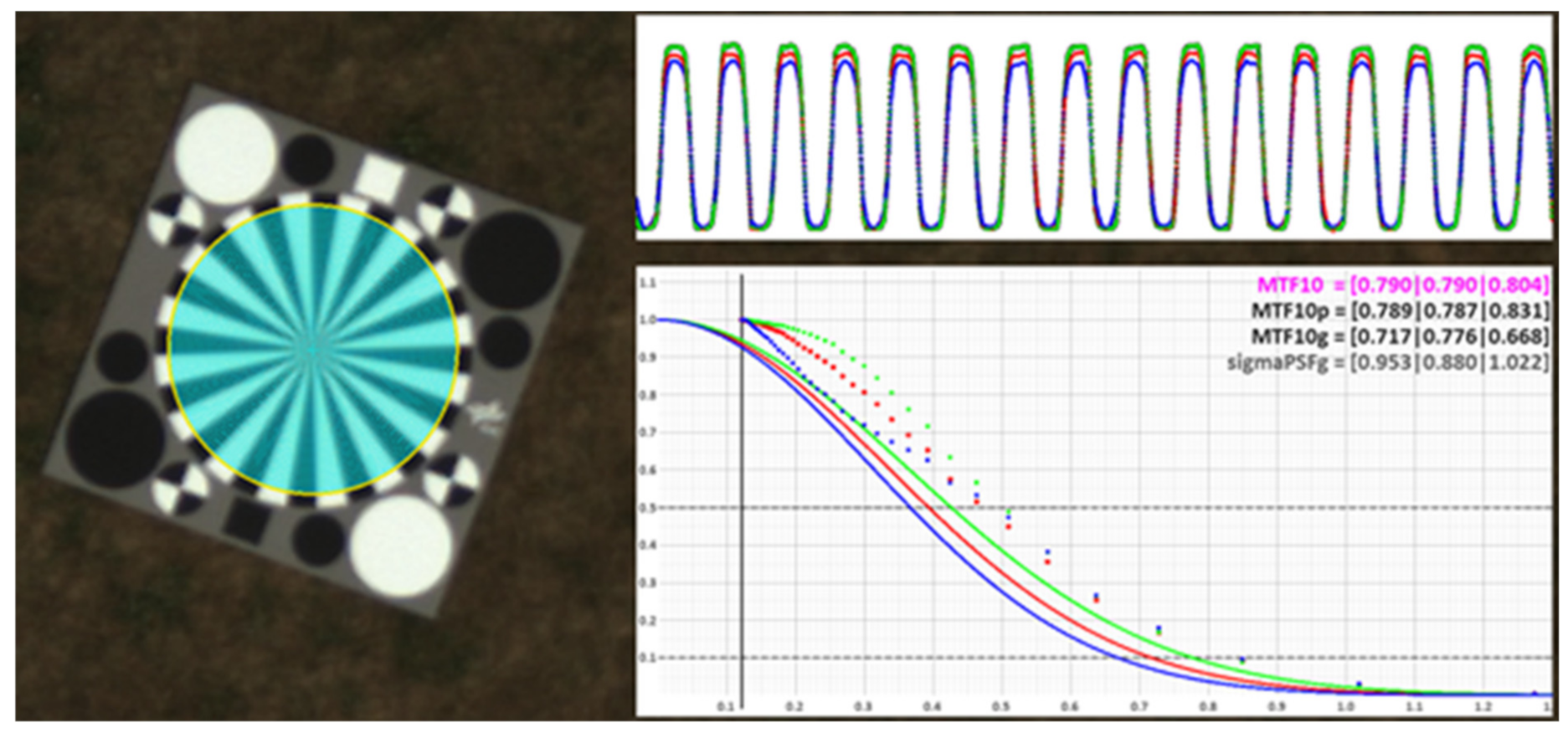
15] is one of the latter approaches. There, the contrast transfer function (CTF) and subsequently MTF is calculated for images with a designated test pattern (e.g., Siemens-star, see
Figure 1).
According to the above-mentioned approaches, the smallest recognizable detail or “the resolution limit is reached if the distance between two points leads to a certain contrast in image intensity between the two maxima.” [
16]. Using a priori knowledge of the original scene (well-known Siemens-star target) CTF, MTF and PSF can be approximated, e.g., by a Gaussian shape function [
17] or polynomial function. Coordinate axis for CTF and MTF is the spatial frequency
(Equation (3)) and is calculated as the quotient of target frequency
divided by current scan radius r multiplied by π. Target frequency
is constant and equivalent to the number of black-white Siemens-star segments. Related (initially discrete) values for contrast transfer function
are derived using intensity maximum
and minimum
for every scanned circle (Equation (4)). Simultaneously, the function value is normalized to contrast level
at spatial frequency equal to 0 (infinite radius). Continuous function values
are either derived by fitting a Gaussian function into discrete input data or, e.g., a fifth order polynomial. According to [
18], the obtained CTF describes the system response to a square wave input while MTF is the system response to a sine wave input. The proposed solution is a normalization with
followed by series expansion using odd frequency multiples (Equation (5)).
There are several criteria specifying the resolving power of camera systems. The parameter σ (standard deviation) of the PSF (assuming Gaussian-shape) is one criterion. It directly relates to image space and is an objective measure to compare different camera performances. Another criterion is the width of PSF at half the height of its maximum (full width half maximum—FWHM).
The value for MTF at 10% modulation contrast often is referred to as resolution limit or cut-off frequency of MTF
= 0.10 at spatial frequency
where its reciprocal
(PSF) corresponds to the least resolved scale in image domain. This scale factor multiplied by nominal ground sample distance (GSD) then delivers the least resolved distance and is named ground resolved distance (GRD) [
19,
20,
21,
22].
4. Accuracy Aspects and Ground Control Network
To achieve the highest positional and vertical accuracy of the ground control network, many aspects must be considered. Since the highest requirement is given by the expected internal accuracy of the photogrammetric block, the expected accuracy is in the range of the GSD, i.e., approx. sxy ≈ GSD = 0.9 mm. This means that for a reliable accuracy test with a simple rule of thumb a network accuracy of sxy = 0.3 * GSD ≈ 0.3 mm must be achieved. With an extension of the rail area, including ancillary areas, of 30 × 330 m outdoors, the target accuracy, which results from the tolerances for the rail position discussed above, is difficult, if not impossible to maintain. Assuming the same rule of thumb, the target accuracies σxy = 2.5 mm, and σz = 25 mm result in values for the network measurement of σxy’ ≈ 1 mm, and σz’ ≈ 10 mm. Given modern geodetic surveying equipment and applying state-of-the-art adjustment methods, this accuracy could be achieved. This would mean that we could verify whether the photogrammetric image block is good enough to check the tolerances of the rail, but we cannot exploit the full accuracy potential of the drone-based image block. Practically, to ensure a largely automatic workflow in the photogrammetric evaluation and to guarantee high point measurement accuracy, coded markers were used as ground and check control points.
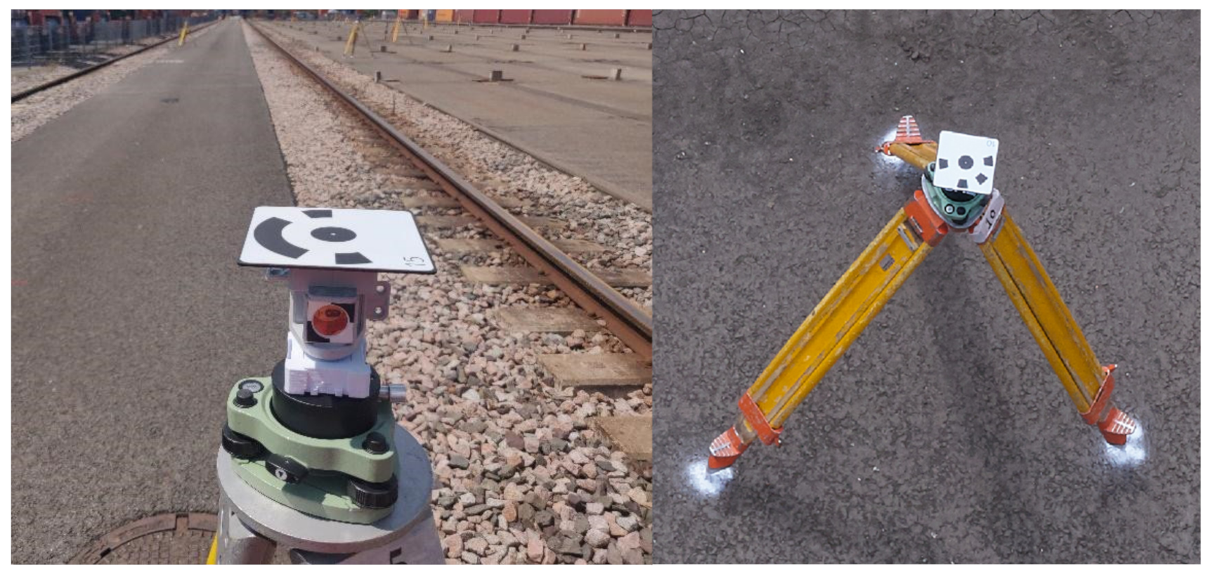
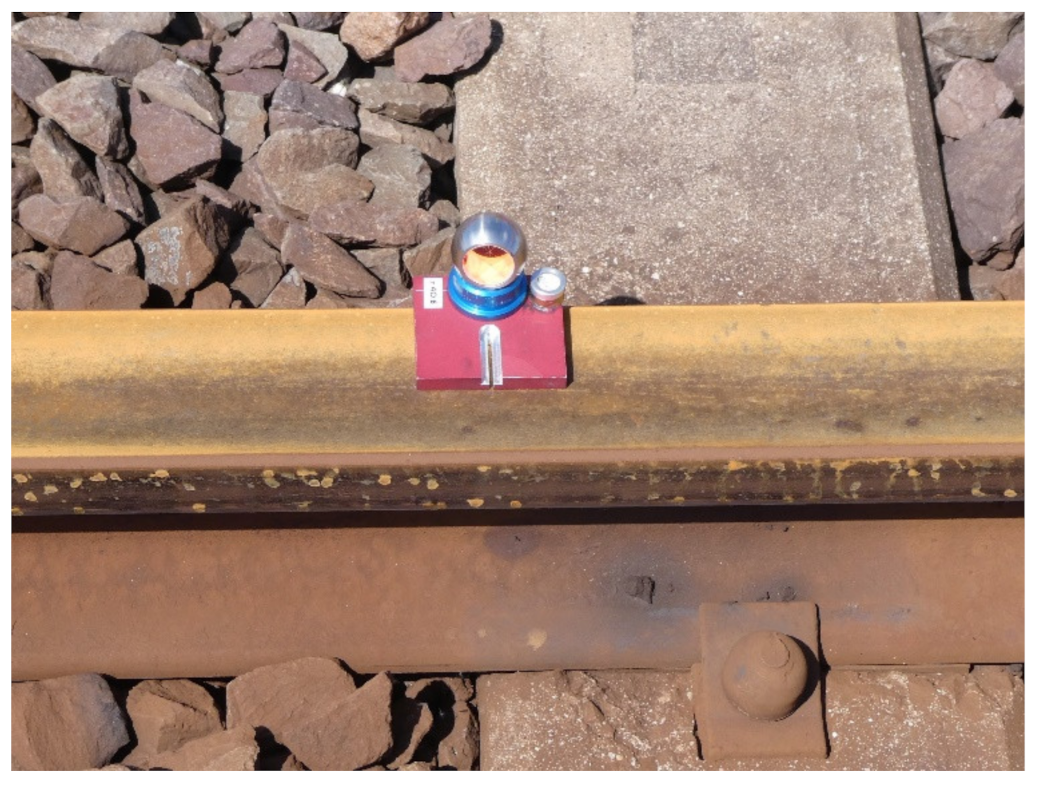
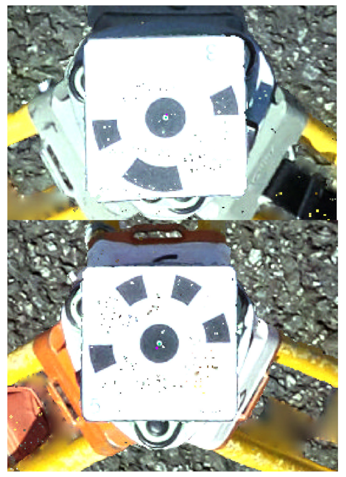
In CTA3, a combination of leveled prism and coded target mounted on the top of the tripod was used in comparison to two prisms and one target used in CTA1 [
1], see
Figure 2. By this procedure, the number and time of the measurements from each station were reduced significantly. The prism and the center of the marker are arranged on one axis and the distance is calibrated. By measuring the prism, the position and height of the center of the marker can, therefore, be determined by adding the known height offset. The prisms must be leveled in order for the vertical positioning of the marker setup to be guaranteed. Twenty such combinations of prisms and targets were produced and attached to tripods, which thus could be leveled on the one hand but could also be assumed to be stable over a certain period of time.
One difficulty in surveying this elongated track object is that fixed points are only available quite far outside. A simulation in the run-up to the measurement campaign has shown that the required position and height accuracy can still be achieved under optimal conditions. During the campaign, however, seven pre-determined datum points were visible from the block under consideration, and furthermore, the meteorological conditions were good. The realized network configuration including error ellipses at the 20 ground points (1 × 20 prisms) is shown in
Figure 3.
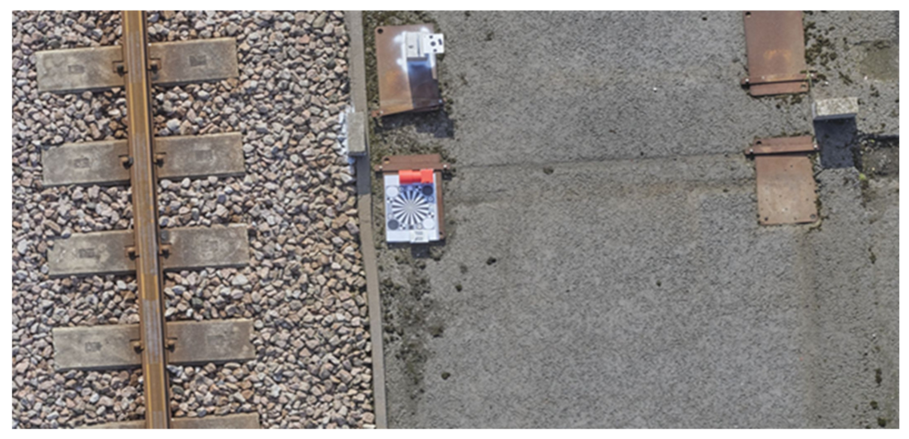
By applying the target detection with the Leica MS50 total station in use, an automated set measurement could be achieved. During CTA1 we had encountered difficulties with the reference data which were captured by a company (using a rail car), but the surveying network was located on different datum points, compared to ours. This has led to some residual deviations between our solutions and the one from the company. To avoid this problem, in the new campaign (CTA3), the edge of the rails was directly measured by employing a rail shoe (
Figure 4) in our own surveying network as a reference. By this means, we could evaluate the result for the photogrammetric solution to a reference within the same reference frame, and hence did not need to cope with unknown deformation caused by a different datum definition.
The network adjustment was carried out using the PANDA software package [
23] and is based on the principle of free network adjustment. This network was then transformed into the seven datum points. After the network adjustment, the above-mentioned computation of the marker coordinates was carried out. This adding of the distance requires a variance propagation so that the accuracies of the extrapolated coordinates can be determined for the photogrammetric targets. On average, a 3D accuracy of 1.1 mm was achieved, in s
xy’ ≈ 0.89 mm and in s
z’ ≈ 0.7 mm in height. These numbers confirm the simulation result, and the accuracy is good enough to verify the tolerance of rail location and height, as indicated above.
5. Flight Planning and Data Acquisition
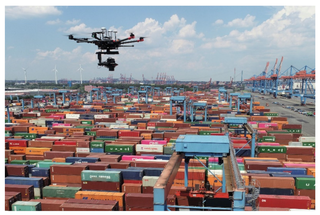
As introduced in the previous section, an industrial UAV, DJI Matrice M600 Pro was employed for carrying the camera needed to perform the survey missions.
Figure 5 shows the system inflight over the survey area. The UAV was controlled using a custom mission planning Android app called Inspekt GS [
24] utilizing the DJI Mobile SDK. This selection allowed us to focus on the main application development rather than the low-level control of the UAV.
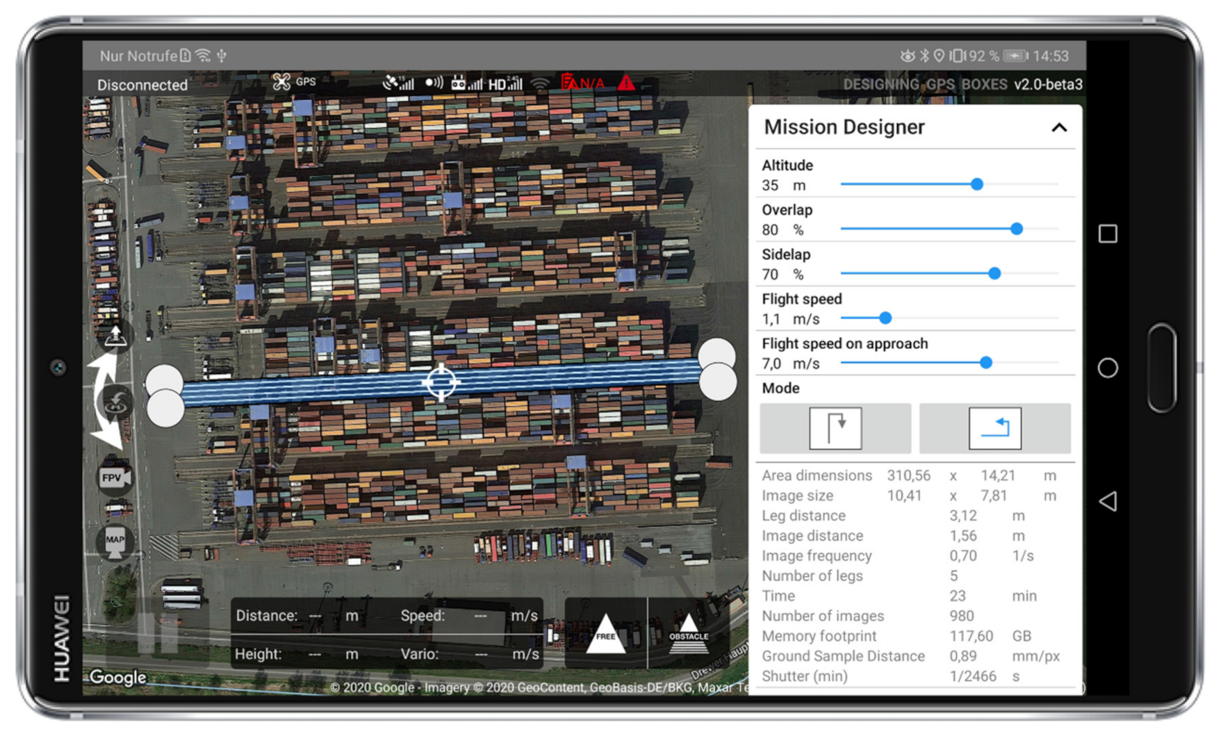
The UAV has a dual antenna differential RTK (D-RTK) setup onboard which gets the correction data from a base station near the survey area. This setup calculates precise heading information of the drone in addition to the primary magnetometer sensor of the UAV. Since the flight environment contains largely metallic containers which are a source of magnetic interference for the magnetometer, the D-RTK setup allowed us to maintain the constant heading without any issues. The RTK position is also saved in the camera images using the EXIF tags. This is needed in the next step of data processing and will be explained in the next section. Usually, for survey missions, the UAV flies in strips, maintaining an along-track and an across-track overlap. This pattern was implemented in the Inspekt GS. A typical mission plan is shown in
Figure 6.
To avoid the motion blur, the camera should not move more than 0.5 pixels for the duration that the lens shutter is open. The following formula results to calculate the mission speed:
Based on a GSD of 0.9 mm and a minimum shutter speed of 1/2500 seconds, a very low flying speed of 1.1 m/s was obtained. In our specific application though, we also had the challenge of moving cranes in the field of view of the camera. Since the motivation of the research project was to carry out the survey in an operating container block, cranes would be encountered during the mission flight. An analysis was carried out with three datasets in a moving block. It was found that in the complete block approximately 10% of the region was blocked by the presence of the moving cranes. To solve this problem, a modular mission planning was implemented in Inspekt GS along with the integration of the crane movement information from three different sources. These sources are:
- (1)
Computer vision-based crane detection from the live video feed of the primary camera.
- (2)
RTK-equipped boxes placed on top of each crane in the measurement block transmitting their location in real time over Cellular 4G connection to Inspekt GS
- (3)
Manual button in the app to provide input from an operator observing the crane movements.
All these methods are complementary to each other and depending upon the requirement, one method is chosen over the other. During a typical flight mission, when a crane is found to be occluding the rails, this area is marked as invalid and scheduled for a future re-flight. Once the first mission is over, the invalid areas are collected together, and a re-flight mission is planned to survey only these areas. This process is repeated until the complete block is captured with images without occlusion from the cranes. If the battery is not enough for direct re-flight of the blocked areas, autonomous landing is performed at the launch position, and batteries are exchanged. Since all the images so obtained are processed in a single batch, it does not affect the reconstruction process.
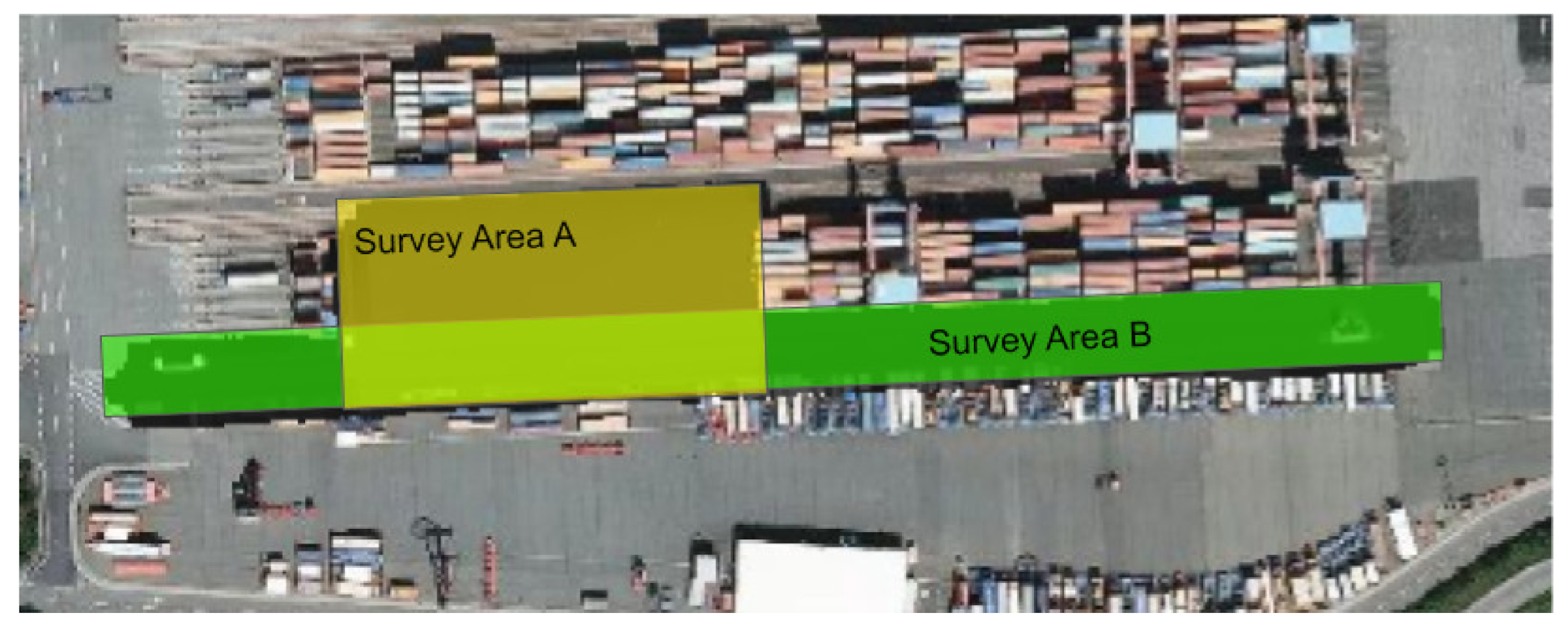
Figure 7 shows the flight areas which were surveyed during CTA3. Due to regular maintenance activities, this block was free from the containers hence it was possible to carry out unrestricted measurements and flights.
The yellow marked survey area A was 100 m in length but contained the north and south side rails of both the cranes operating on this block. This area was chosen to carry out experiments with a different camera lens, sidelap, overlap, and flight heights.
The green marked survey area B was the usual full block area. However, it contains only the south rails of both the cranes operating in this block. Since the 300 m length of the survey area is a challenge both for the ground survey of markers and photogrammetry, the datasets on this area allow for testing the limits of the concept.
6. D Reconstruction of Rail
The dataset acquired as described in the previous section is processed using the photogrammetry software Agisoft Metashape. As a first step, the images are aligned using the EXIF tags containing the capture locations. After this step, the automatic detection of the GCP is carried out. Since the GCPs are as per the Agisoft standard, the software can detect the markers without manual input. This reduces potential manual errors. The data related to the survey measurements of all the detected markers is imported into the Metashape and re-optimization of the cameras is done based on this new information. This leads to a globally corrected sparse point cloud and densification can be done now. A digital elevation model (DEM) is then extracted from the dense point cloud which is used as the main input for the extraction of rail edges. The approach requires the DEM, which contains the 2.5D information for the study area or the point cloud. A custom software named Inspekt-XT was developed for this task using the Python programming language. In this software, two methods were implemented which are described next.
Method 1: Section profile method.
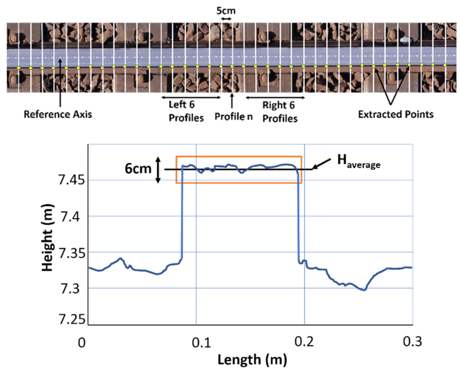
This procedure aims to extract the edges and centers of the rails from the DEM or the point cloud. For this purpose, profiles are created at 5 cm, perpendicular to the rail direction. The position of the profiles and an exemplary profile are shown in
Figure 8. The value of 5 cm interval arises from the consideration that although a high number of sections allows for better understanding of the rail position and hence is desirable, this also leads to higher processing times.
Since the dense image matching on the rail section can lead to faulty points, only profiles that scatter in the upper area by less than +/−3 cm from the mean value are considered. From the valid profiles, the lower points that are directly adjacent to the edge are then extracted. The points from the six adjacent profiles on both sides are used to create a straight line to further reduce the influence of matching errors (see
Figure 6, above, yellow points).
The reference axis for each rail is specified by Hamburger Hafen und Logistik AG (HHLA), see the dotted axis in
Figure 8 (upper). The actual position is determined from the averaged profile points over half the specified rail width.
Method 2: 1D Convolution method.
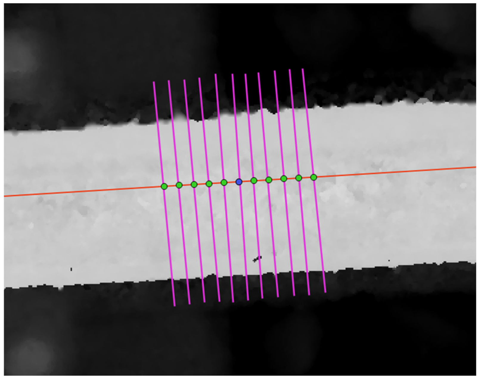
Another method based on 1D convolution on cross-sectional elevation (derived from DEM) values to determine the right and left edge was used. In this method, profiles are created at a distance of 2 m, perpendicular to the rail direction. The locations of the profile can be determined in two ways, firstly they can be located such that they coincide with the field survey points (HHLA reference points or shoe points measured by Sokkia). This method helps to compare directly the calculated deviations from actual measured deviations of given field reference points. Secondly, the profiles can be located independently at uniform intervals along the rail. This is done after validation of the method, specifically for analyzing new tracks for which ground survey data are absent. To avoid any inaccurate or false elevation value derived from the DEM at the profile location, we resorted to averaging the elevation values across multiple profiles in a 10 cm (5 cm on either side of the considered profile) interval for each profile along the rail,
Figure 9.
The next step in the process is the 1d convolution operation. The aim was to detect the rising edge and the falling edge, which would give locations of the points along the profile line indicating the left and right edge of the track, respectively. In this article, the first method was used to process the data and visualize the results and the second one was used only for validation. However, method 1 was developed with much more effort and automation in mind to be able to do many experiments very fast. The method 2 was developed for the verification of method 1.
Processing Times
The dataset from survey of one block results in roughly 400 images (using 80 mm lens) which has a total size of 120 gigabytes. To process such huge dataset, a high-end Workstation with 32 Core Intel Xeon 6154 CPU, 384 GB RAM and two Nvidia RTX 2080 Ti graphics cards was used. The reconstruction process on this machine using Agisoft Metshape software happens in an automated way and takes 36 h. The further extraction of the rail using Inspekt-XT software takes a few minutes.
7. Results
This section describes the results obtained from the datasets acquired during the test campaign, which took place at the CTA, Hamburg in June 2020 (CTA3). A free block was chosen for this campaign, whose rails had been renewed shortly before the campaign and in which, therefore, no containers were placed. Conventional position measurement of the rails was carried out with the rail shoe using Sokkia Total station. The results are compared with those of the method developed here. The system flights were carried out outside of the operation of the cranes as well as during operation, mainly to test the approach to the detection of the cranes, which will not be discussed further here.
7.1. Impact of Ground Control Points
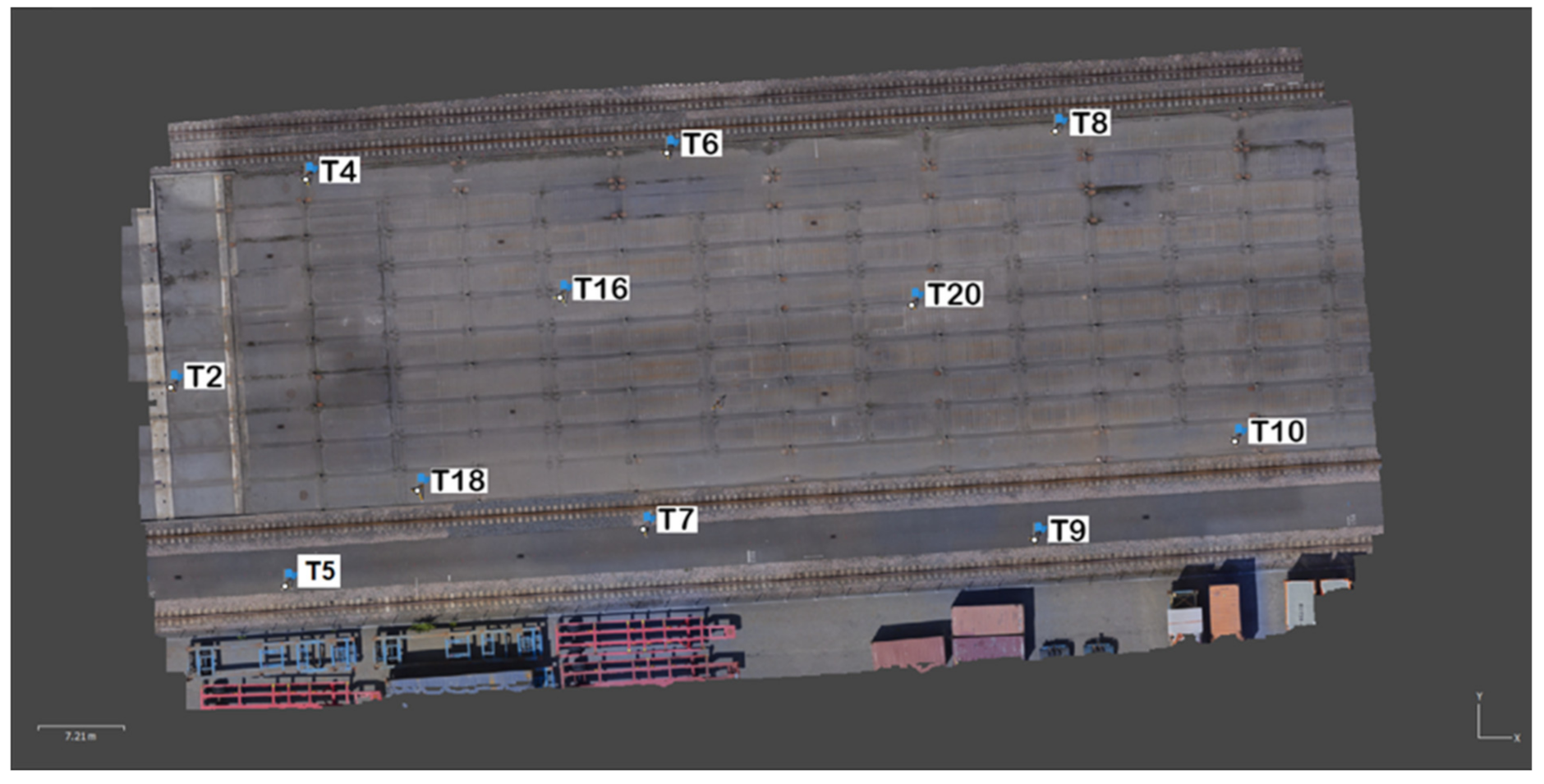
One dataset of the area A was processed using a different set of GCPs to evaluate the impact of the structure and quantity of GCPs on the bundle adjustment accuracy and hence, on the final extraction results,
Figure 10.
For this purpose, the bundle block adjustment was performed using different constellations of GCPs and CPs. GCPs are needed to cover the area of interest and in this research, the GCPs were used to have the most control on the accuracy of the block which covers almost a flat area. The first setting (a) used seven GCPs and four CPs with a total error of 1.9 mm (
Table 1) while the second setting (b) used four GCPs and seven CPs. The total error of GCPs of setting (b) shows a slight decrease in comparison to the error of GCPs of setting (a) but the error of CPs was around 3 mm. However, the error of CPs in the second setting (b) shows a greater value than the setting (a) and was 5.5 mm. In order to further understand the effects of different settings, we take a closer look into the railway geometry.
Hence, the DEMs for each setting were generated and processed to extract the railway edge points. These points then were compared to the reference points. The results of the comparison have clearly shown that the number and the distribution of the ground control points affected the accuracy of the bundle block adjustment and hence, the quality of the generated DEMs and the extraction results.
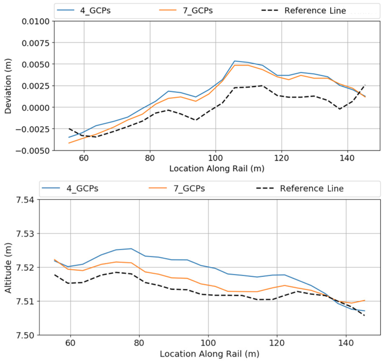
Figure 11 reflects this conclusion and shows that setting (a) has achieved the best results for XY deviation to the reference measurements with RMSE = 1.9 mm in comparison to RMSE = 2 mm for setting (b),
Table 2.
A similar trend but with a more clear effect of reduced number of GCPs is seen for the elevation values to the reference measurements with RMSE = 3.1 mm for the setting (a) in comparison to RMSE = 6.2 mm for setting (b).
This shows us the number of GCPs reduced from the processing, the average error of the bundle adjustment increases, and hence, the position and altitude deviations to the reference points increase (
Table 2). It should be noted though that the increase in error from setting (a) to (b) is drastic and this can be attributed to the fact that in setting (b) only four GCPs are used which is the minimum needed to correctly transform coordinates from one system to the other, block deformation effects cannot be mitigated.
7.2. Surface Modelling and Ortho-Projection
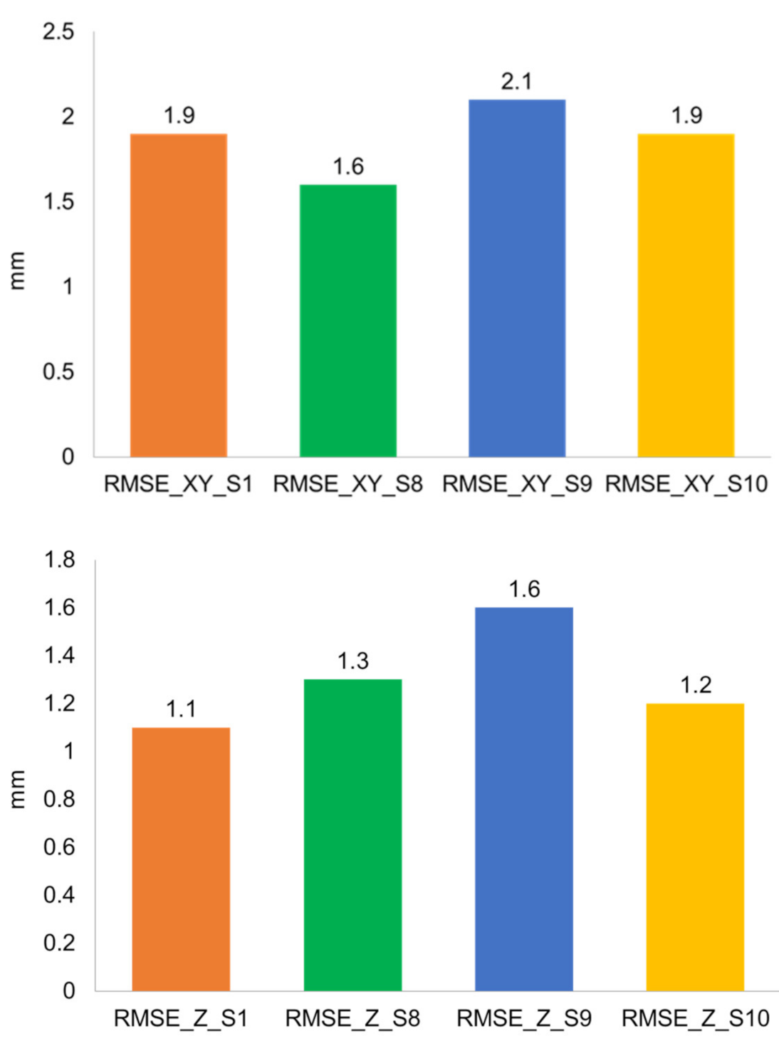
The rail position is detected directly via the digital 2.5D height model (DEM) derived from the dense image matching. Furthermore, data are also superimposed with a generated (true) orthophoto (TOP), for example for visual checks and superimposition with other georeferenced data. For these reasons, it is important to quantify how accurate these derived products are. Sources of error during processing are deposits or “holes” in the point cloud, for example in low-contrast regions. Such artifacts directly affect the quality of the DEM. Furthermore, the quality of the ortho-projection depends on the surface modelling via the known relations (relief offset). To quantify the geometric accuracy of the products DEM and TOP, prominent points (the given, marked ground control points), but also points manually introduced into the BBA (clearly defined corners) were measured in the ortho image, respectively, in DEM that are generated using a different camera and flight parameters (
Figure 12).
The settings are described in
Table 3 and the RMSE results of the processing are shown in
Figure 13. As
Figure 13 has shown, the average error between the automatic detected and the manual points is an average of 2 mm approximately for the position and an average of 1.3 mm.
7.3. Effective Spatial Resolution
During the campaign, a Siemens-star has been included in the scene and the effective spatial resolution can be determined (see
Section 3.3,
Figure 14). Values for MTF10 have been measured and calculated for four aerial images depicting the Siemens-star located in different areas of the image.
As a side note, all images have been sharpened during raw-image-to-color-image conversion (de-mosaicing). The outcome of this sharpening process is accentuated edges, but the impact that these sharpening procedures have on subsequent products (e.g., bundle block adjustment and point clouds) is still scientifically unknown. This issue is part of further investigation. Results are given in
Table 4.
All measurements deliver very similar results. Values for MTF10 are between 0.943 and 1.082 (Nyquist frequency is 1.000). This is a variation of less than 13% and it can be concluded that the effective spatial resolution is loss-less compared to theoretical resolution.
7.4. Measuring the Rail Position and Discussion
Based on the image block and the BBA with the best results, a DEM of area B was created. According to the methodology presented above, rail points could be extracted and the difference to the reference line calculated. The quality of the DEM and hence the final results were tested by applying different camera and flight setups. In this context, different camera objectives, mission speed, and sidelap were tested. Finally, statistical values of the XY and altitude deviations to the centerline were calculated which are presented in the
Table 5.
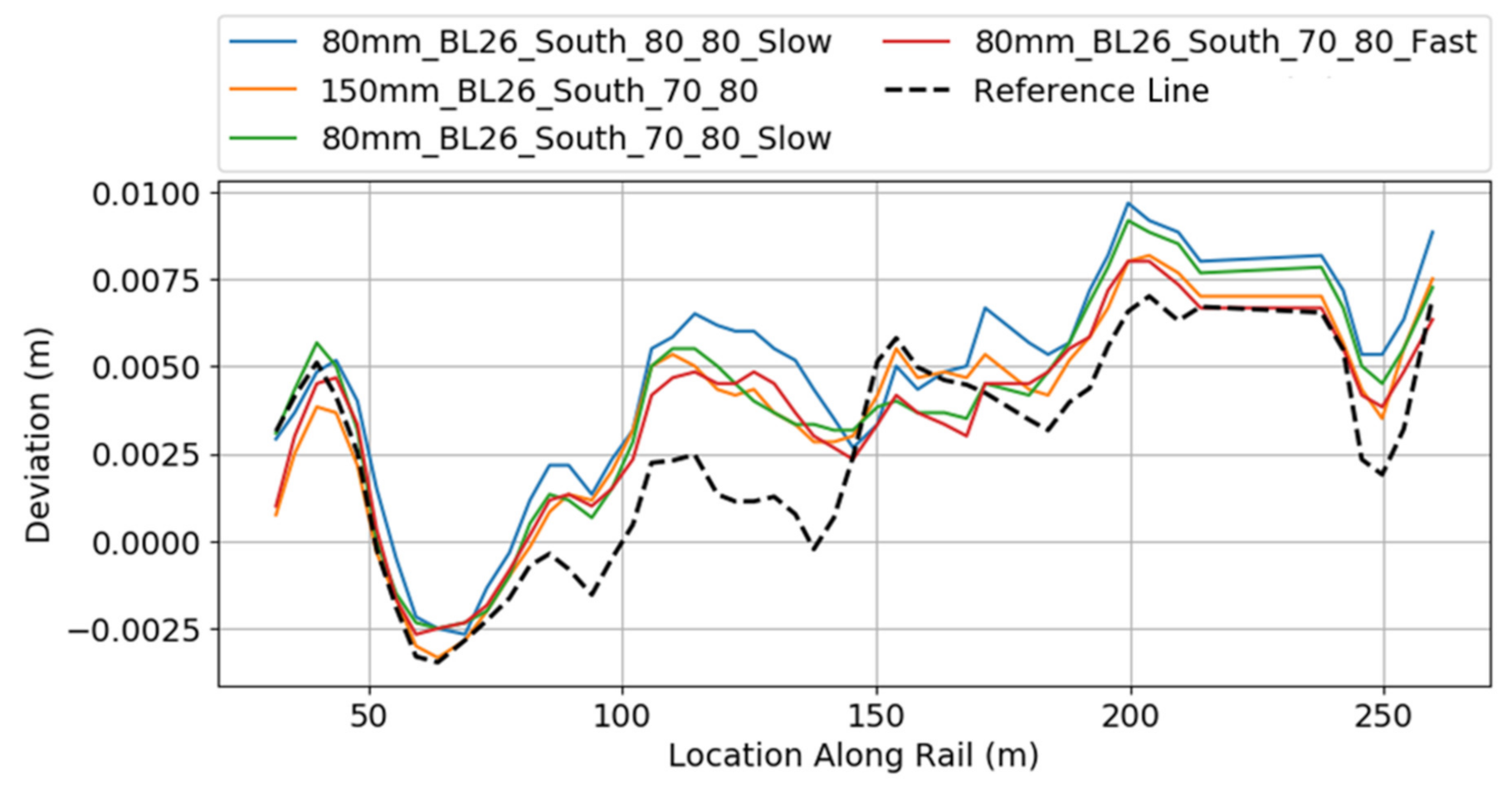
Figure 15 shows the comparison of deviation in XY for these different settings. In this figure, the different continuous lines show the deviation from the reference line as a function of the position along the rail, taking into account the distance determined in this project. The dashed line is the distance calculated by the rail shoe reference measurements. Qualitative analysis of
Figure 15 shows an insignificant variation in the results irrespective of the flight setting used.
Moreover, these results also show that similar results are expected if the 80 mm lens is used with a GSD of 1.6 mm instead of the 0.9 mm for the 150 mm lens. This has significant implications on the mission flight time and the total dataset size for the survey area. This is because the 80 mm lens allows a faster mission speed of 1.9 m/s which is almost twice as fast as the maximum mission speed with a 150 mm lens. Therefore, the mission can be completed in almost half the time. Moreover, a quick calculation of the dataset size shows that this is also reduced by half resulting in reducing the processing time from 2 days for a 150 mm lens to 1 day. Additionally, the figure shows higher deviations between the reference line and the result lines close to the middle part of the railway (between 70 and 150 m) compared to the first and the last part of the railway. The explanation of this deviation is that the reflectivity of the railway at that part is higher than the one at the beginning and the end part. This part is heavily loaded and hence, the rust is removed, and the surface becomes more shinny than the rusty parts on both sides around the middle part causing noise that affects the final results.
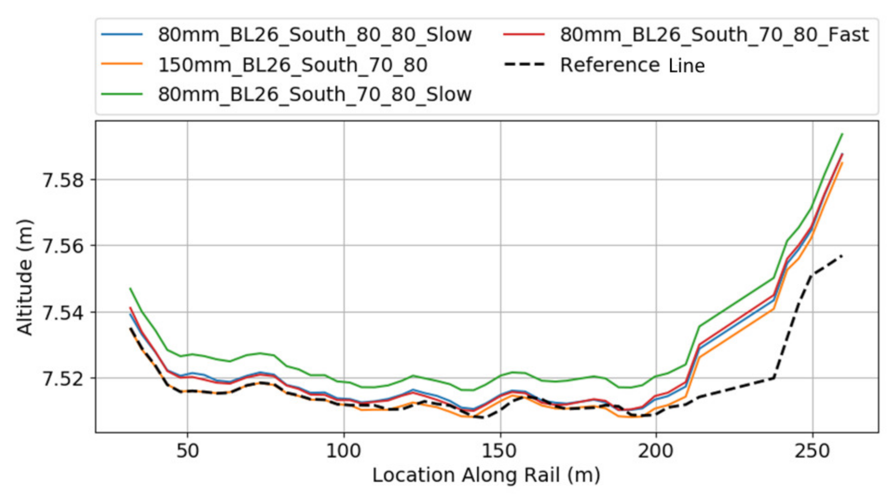
Figure 16 presents the elevation results for the same settings. Here, the observations are also the same as that of the previous figure.
In
Figure 16, the elevation profile is plotted, again separated according to our results and classical surveying. The “ramps” at the beginning and at the end of the track, where a height difference of 5 to 7 cm is visible, can be observed well in both profiles. A technical explanation for these ramps is that the rails are not loaded at the ends because the cranes do not drive into this area.
The curve is much smoother than that of the location. From the figure, it can clearly be seen that the differences between the continuous lines and the dashed line increases close to the waterside.
8. Conclusions
This paper presented the results of the final test campaign of the research project AeroInspekt for automatic measuring of the crane tracks using a high-resolution medium format camera system installed on a multicopter. In this campaign, the procedures of the measurements to achieve the required accuracy were continually improved. The improvements included the concept of the ground control points to reduce the time of surveying and to overcome related conflicts with the crane schedule. In addition, the rail shoe measurements were performed as a reference to ensure that all the measurements have the same datum. The usage of the different camera lens and UAV speed parameters have shown that we can achieve similar results by using an 80 mm lens instead of a 150 mm lens. Hence, mission flight time and total dataset size can be significantly reduced. The processing workflow of the dataset is automatically performed, including measurement of signalized ground control points in the images. Furthermore, only the DEM and the reference points of the centerline are needed to automatically extract the rail track profiles and calculate the deviation to the centerline. The results have shown that the deviations to the reference line are similar for 150 mm and 80 mm lens with 2 mm error in position and 8 mm error in altitude for 150 mm lens and 14 mm error in altitude for 80 mm lens, respectively. The UAV-based photogrammetry method to measure the actual location of the rail was proved to be a reliable method and can be performed without interruption of the crane movement. To our knowledge, we developed and tested, for the first time, a state-of-the-art photogrammetry-based workflow to fully automatically derive the outline of an elongated track system. Through comprehensive ground survey measurements, we could prove that the desired accuracy level, required by the crane operator, can be maintained and that we can deliver data in the same quality range as a reference method. The method for automatic rail delineation was developed and tested; using two different methods, we could cross-validate its accuracy and quality. In comparison to the current measurement technique which takes a complete day for inspecting one block and during this period the activities in the block are stopped, our method requires only 1.5 h inside the block for the distribution of the ground control points, 30 min flight time and 36 h automated processing time. As attested by the container terminal, this is a significant time and revenue saving for them and they are planning to bring the technology developed during the project into operation as soon as possible.
For future projects with the aim to exploit the very high resolution and accuracy offered by modern UAV-based photogrammetry, we suggest checking the following in particular: concerning lighting conditions, it is important to take care that diffuse illumination is available during flight. Direct light has unfavorable influence on dense matching quality, and strong shadows hinder observation as well. On the other hand, if it is too cloudy, the balance between aperture and exposure time might lead to restricted depth of field or image blur, respectively. The trade-off between the possible inner image block accuracy and the verifiable, actually derived exterior accuracy, also with respect to the datum is obvious when we reach GSD-levels in mm-range. Special attention is needed regarding a valid geodetic control network, proper measurement, signalization of targets and automated image measurements. With regard to the choice of the optimal lens, we saw that the better nominal GSD delivered by the 150 mm lens, compared to the 80mm lens, is not fully reflected in the final results. Because of better aperture values, the 80 mm lens is less sensitive to image sensor noise, and the DSM around the elevated rails is better, probably because of the larger opening angle. Those might be reasons why the effective accuracy of both systems does not differ significantly, at least in terms of XY.

 ,
, 


