Towards Semantic SLAM: 3D Position and Velocity Estimation by Fusing Image Semantic Information with Camera Motion Parameters for Traffic Scene Analysis

Abstract

In this paper, an EKF (Extended Kalman Filter)-based algorithm is proposed to estimate 3D position and velocity components of different cars in a scene by fusing the semantic information and car model, extracted from successive frames with camera motion parameters. First, a 2D virtual image of the scene is made using a prior knowledge of the 3D Computer Aided Design (CAD) models of the detected cars and their predicted positions. Then, a discrepancy, i.e., distance, between the actual image and the virtual image is calculated. The 3D position and the velocity components are recursively estimated by minimizing the discrepancy using EKF. The experiments on the KiTTi dataset show a good performance of the proposed algorithm with a position estimation error up to 3–5% at 30 m and velocity estimation error up to 1 m/s.

1. Introduction

In recent years, significant progress has been made in vision-based Simultaneous Localization and Mapping (SLAM) to allow a robot to map its unknown environment and localize itself in it [1]. Many works have been dedicated to the use of geometric entities such as corners and edges to produce a dense feature map in the form of a 3D point cloud. A robot then uses this point cloud to localize itself. The geometric aspect of SLAM has reached a level of maturity allowing it to be implemented in real time with high accuracy [2,3] and with an outcome consisting of a camera pose and sparse map in the form of a point cloud.

Despite the maturity and accuracy of geometric SLAM, it is inadequate when it comes to any interaction between a robot and its environment. To interact with an environment, a robot should have a meaningful map with object-based entities instead of geometric ones. The robot should also reach a level of semantic understanding allowing it not only to distinguish between different objects and their properties but also to distinguish between different instances of the same object.

The required granularity of semantic understanding, i.e., object or place identity, depends on the task. For collision avoidance, it is important to distinguish between different objects while distinguishing between different instances of the same object may not be required. In contrast, robots manipulating different instances of the same object, like in warehouses, should have a deeper level of understanding allowing them to distinguish between different instances of the same object and their geometric characteristics. Semantic understanding can sometimes be considered as place understanding instead of object understanding: A robot that moves among different kinds of places (room, corridor, elevator, etc.) should be able to distinguish between them.

In autonomous driving, traffic scene analysis is a crucial task. An autonomous vehicle should not only understand the position of different objects but should also be able to predict their trajectory, even in the case of occlusion. Over the last years, traffic scene analysis has leveraged the maturity of deep learning approaches to detect different objects in the scene. The improvements in deep learning-based 2D object detection algorithms [4,5] enable a better understanding of scene content. However, they do not allow us to have a 3D description of the scene. Therefore, recently, many works have been devoted to augment the results of 2D object detectors to obtain a 3D representation of the scene in the form of 3D coordinates of the cars in the scene.

A number of recent works in 3D representation of cars in a scene [6,7,8,9,10,11,12,13] utilize prior information about 3D Computer Aided Design (CAD) models of the cars. After the cars in a scene are detected using a 2D detector, they are matched against a set of 3D CAD models to choose the corresponding models. Then, a virtual (calculated) image for the scene is generated using the 3D CAD models of the detected cars. After that, the virtual image is compared with the actual image captured by the camera and the discrepancy between the two images is calculated. The cars’ poses are estimated by minimizing the discrepancy between the virtual and actual image. These works can be divided into two groups depending on the way they compute the discrepancy between virtual and actual images. One group computes the discrepancy as the difference between two contours space [7,10]. The first contour represents the virtual images generated using the 3D CAD model while the other contour represents the corresponding detected car in the scene. The second group computes the discrepancy as the difference between some key points (such as window points, wheels, etc.) in the virtual and actual image [6,11,12,13,14]. It was found that this approach led to more accurate results than the contour approach [9].

Regardless of the approach used to compute the discrepancy, such works have two drawbacks. The first drawback is that they estimate the pose of the detected cars only and do not give information on velocities. The second drawback is that they produce a one-shot estimate that infers each frame separately and does not take into account the temporal dynamic behavior of the objects between successive frames. The dynamic behavior of different objects is important for trajectory prediction, especially in the case of full occlusion.

The previous drawbacks inspired us to introduce an approach that has the following contributions:

• Unlike previous approaches that are end-to-end data driven solutions, we introduce a hybrid solution that, on one hand, leverages deep learning algorithms to detect different cars in the scene and, on the other hand, describes the dynamic motion of these cars in an analytical way that can be used within the framework of a Bayesian filter where we fuse the discrepancy between the virtual image, obtained using a 3D CAD model, and the actual image, with camera motion parameters measured by the sensors on board. In this way we estimate not only car positions but also their velocities, which is important for safe navigation;
• Our approach will be able to keep predicting the motion parameters of the cars even in the case of full occlusion because we involve the dynamics of their motion in the estimation process. Previous approaches cannot predict the position of the car in the case of full occlusion.

The rest of the paper is organized as follows. Some important related works are discussed in Section 2. In Section 3, we go through the proposed approach describing its main components. Section 3.2 introduces the mathematical problem statement used in our approach and its solution using EKF (Extended Kalman Filter). Section 4 and Section 5 present experiment results and a discussion about the proposed algorithm, respectively. Finally, we present our conclusions in Section 5.

2. Related Work

In the following lines, some works related to 2D object detection, semantic SLAM without using a 3D CAD model, and image-based 3D object detection using a 3D CAD model will be discussed.

2.1. 2D Object Detection

Identifying objects is a crucial step in the semantic SLAM pipeline. Therefore, we use the state-of-art in deep learning to detect and identify the objects. There is a trade-off between the speed and accuracy of Convolution Neural Networks (CNN) used in object detection. On the one hand, techniques such as R-CNN [15], Fast R-CNN [16], and Faster R-CNN [17] are accurate. They are region-based techniques that first produce candidate regions containing some potential objects and then classify these objects. Although accurate, they are computationally expensive and are not suitable for real time application. On the other hand, bounding boxes-based techniques such as You Only Look Once (YOLO) [4,18] and Single Shot Multibox Detector (SSD) [5] are less accurate but are suitable to real-time applications. In this paper, we will use YOLOv3 [18] as an object detector because it is considered as the-state-of-art in bounding boxes techniques and it supports both CPU and GPU implementations.

2.2. Semantic SLAM without Using 3D CAD Model

In recent years, a few works have been dedicated to semantic SLAM without using a prior 3D CAD model. Bowman et al. [19] used an Expectation Maximization algorithm to optimize the joint distribution of camera pose and detected objects locations. Doherty et al. [20,21] addressed the problem of data association in semantic SLAM. In [20], the authors decomposed the problem into a discrete inference problem to estimate the object category and a continuous inference problem to estimate camera and object location. In [21], the authors proposed a proactive max-marginalization procedure for the data association problem in semantic SLAM. Unlike the previous works which did not benefit from a prior knowledge of some objects, in our approach we use prior known models of the objects.

2.3. Image Based 3D Object Detection Using 3D CAD Models

In [22], Davison argued that 3D object model fitting is an active choice to produce high level semantic mapping. Many works have been dedicated to utilize prior information about the 3D model of the object. Chabot et al. introduced one of the pioneering works for 3D object detection from monocular camera images [6]. Their approach consists of two phases. In the first phase, they used a cascade Faster R-CNN to regress 2D key points of the detected car and produce a template similarity. In phase 2, they selected the matching 3D CAD model from the database based on the template similarity obtained in the first phase. Having a 3D CAD model and the corresponding 2D key points, they used Efficient Perspective-n-Point (EPnP) [23] algorithm to compute the discrepancy and estimate the poses of the detected cars. Kundu et al. estimated the shape and the pose of the cars using “Render-and-compare” loss components [7]. They rendered each potential 3D CAD model with OpenGL and compared it with the images of the detected cars to find the most similar model. However, this approach is computationally heavy. In [12], Qin et al. regressed 3D bounding box’s center from a 2D image using sparse supervision. They did not use any prior 3D CAD models. Barabanau et al. improved the previous approach by using a 3D CAD model to infer the depth to the detected cars [13]. Wu et al. [8] extended Mask R-CNN by adding customized heads, i.e., additional output layers, for predicting the vehicle’s finer class, rotation, and translation. None of the previous approaches take into account the dynamic nature of the moving cars from frame to frame. Therefore, in our approach, we extend their works by fusing the output of the object detector with the motion parameters to estimate the position and velocity of different cars in the scene.

3. Proposed Approach

Our proposed approach aims to have a 3D semantic representation of the traffic scene by estimating the 3D position and velocity components of different cars in the scene. It leverages the advances in deep learning-based algorithms to detect the semantic class and different important key points of different cars in the scene. Then, the detected key points are fused with the motion parameters of the camera, i.e., linear velocity and angular velocity, measured by sensors on board to get a 3D representation of the scene with respect to the ego car frame. This section will introduce, first, the proposed pipeline. Then, the mathematical problem statement and its solution will be presented.

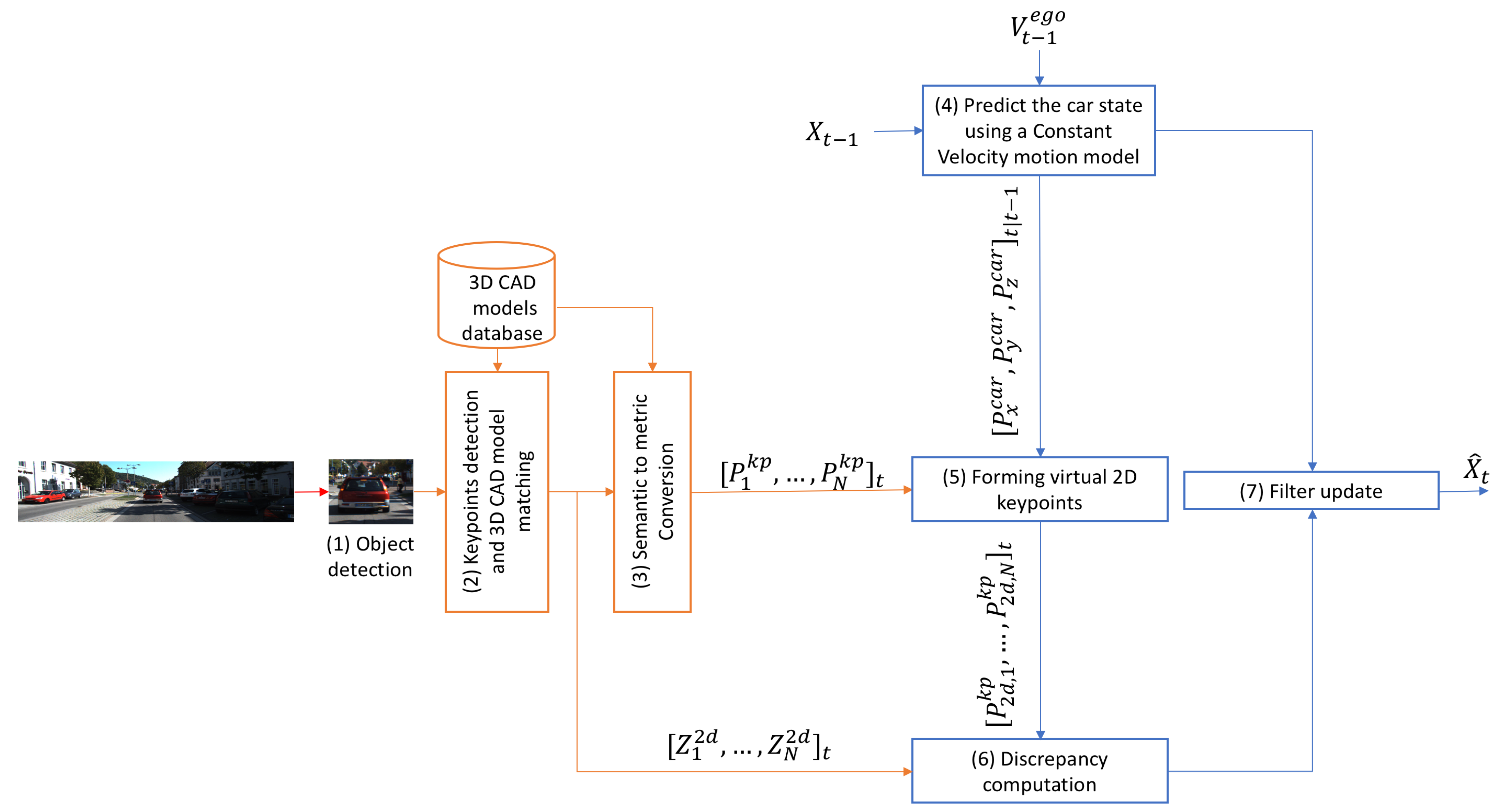
3.1. Proposed Pipeline

Figure 1 illustrates different stages of the proposed approach. In the following lines, we discuss the main steps of the proposed pipeline.

3.1.1. Object Detection

Yolov3 can be used for object detection [18]. Yolov3 is much faster in comparison to other object detection algorithms while achieving comparable accuracy, which makes it very suitable for real time implementation. The output of the object detection algorithm is a number of bounding boxes, each of which contains a detected car.

3.1.2. Key Points Detection and 3D CAD Model Matching

Having a car inside a bounding box, a number of 2D key points can be detected. These key points can be: Rear and front windshield corners, centers of the wheels, the corners of the doors windows, etc. These key points and shape of the car are used to match the car with a corresponding 3D CAD model stored in the database [9]. The 3D CAD model consists of the 3D coordinates of the key points resolved in the car coordinate frame. Once the detected car is matched correctly with its corresponding 3D CAD model, we have a number of 2D key points and their corresponding 3D points resolved in the car coordinate frame. There are some works that utilized neural networks to do key points detection and 3D CAD model matching [6,7]. However, the configurations and the weights of their implementations are not open sourced. Therefore, in order to use these approaches, one has to reproduce their results and retrain the networks from scratch, which is a time and resources consuming process. In addition, the paper contribution is not related to this part. Our main contribution is the temporal fusing of the detected key points with the motion parameters of the car. Therefore, we decided to get the results of this stage in a manual way.

3.1.3. Semantic to Metric Information Conversion

The detected key points with their associated IDs are matched against their 3D CAD model to get their corresponding 3D coordinates resolved in their car coordinate frame. By doing so, we convert the semantic information (object class, car model, and the identity of the detected 2D key points) to a metric information in the form of a set of 3D coordinates.

3.1.4. State Prediction

At this stage, the motion parameters of the ego car measured by GPS and IMU sensors on board are used to predict the 3D position and velocity components of the detected cars with respect to the car coordinate frame. For state prediction, we have used a motion model presented in (Section 3.2.1).

3.1.5. Forming Virtual 2D Key Points

The key points obtained previously in step Section 3.1.3 are projected on the image plane to get 2D virtual key points. To do so, the 3D key points are represented in the camera frame instead of the body frame. Then, the points are projected into the image plane using the pinhole camera model (see Section 3.2.2).

3.1.6. Discrepancy Formulation

Having a number of true key points from Section 3.1.2 and their corresponding virtual key points from Section 3.1.5, the distance between them can be computed. This distance is called the discrepancy between the true image and virtual image.

3.1.7. Temporal Fusing of the Discrepancy with the Motion Parameters of the Camera (Filter Update)

The detected car 3D position and velocities can be estimated by minimizing this discrepancy. An Extended Kalman Filter (EKF) is used to recursively fuse the discrepancy calculated in Section 3.1.6 with the predicted 3D position and velocity components obtained in Section 3.1.4. In the following section the mathematical problem statement will be discussed in detail.

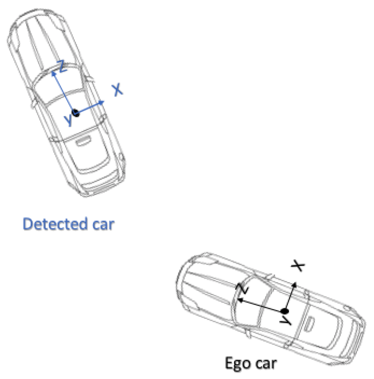
3.2. Problem Statement and Its Solution

Consider a car equipped with a monocular camera and motion sensors moving on a road, capturing successive images for the scene. The cars in the scene are detected using a 2D object detection algorithm like Yolov3. The goal is to estimate the 3D position and the velocity components of each detected car with respect to the ego car (camera) coordinate frame. By doing so, a 3D object-based map for the scene, with respect to the ego car frame, can be created and updated over time.

3.2.1. Motion Model

Suppose $X={[P^{car},V^{car}]}^T$ is the state vector of a detected car (object). It consists of two subvectors: $P^{car}={[P_x^{car},P_y^{car},P_z^{car}]}^T$ is the 3D position of a detected car and $V^{car}={[V_x^{car},V_y^{car},V_z^{car}]}^T$ is the 3D velocity vector. Both vectors are resolved with respect to the ego car coordinate frame and they can be described using Singer’s model as follows [24,25],

$$\begin{array}{cc}\hfill {\dot{P}}_x^{car}& =V_x^{car}-{\tilde{V}}_x^{ego}+v_x,\hfill \\ \hfill {\dot{P}}_y^{car}& =V_y^{car}-{\tilde{V}}_y^{ego}+v_y,\hfill \\ \hfill {\dot{P}}_z^{car}& =V_z^{car}-{\tilde{V}}_z^{ego}+v_z,\hfill \\ \hfill {\dot{V}}_x^{car}& =w_x,\hfill \\ \hfill {\dot{V}}_y^{car}& =w_y,\hfill \\ \hfill {\dot{V}}_z^{car}& =w_z,\hfill \end{array}$$

(1)

where ${\tilde{V}}^{ego}$ is the ego car velocity measured by the motion sensors on-board and used as an input to the model in (1) [26]. $v_i$ and $w_i$, where $i\in [x,y,z]$, are uncorrelated random white noise components. v represents the measurement error of the ego car velocity and the process white noise related to $P^{car}$ while w represents the process white noise related to $V^{car}$. The model in (1) can be written at any time step $\left(t\right)$ in a discrete form as follows,

$$X_t=A{X}_{t-1}-B{\tilde{V}}_{t-1}^{ego}+q\left(t\right),$$

(2)

where

$$A=\left[\begin{array}{cccccc}1& 0& 0& \Delta t& 0& 0\\ 0& 1& 0& 0& \Delta t& 0\\ 0& 0& 1& 0& 0& \Delta t\\ 0& 0& 0& 1& 0& 0\\ 0& 0& 0& 0& 1& 0\\ 0& 0& 0& 0& 0& 1\end{array}\right]$$

(3)

and

$$B=\left[\begin{array}{ccc}\Delta t& 0& 0\\ 0& \Delta t& 0\\ 0& 0& \Delta t\\ 0& 0& 0\\ 0& 0& 0\\ 0& 0& 0\end{array}\right].$$

(4)

${\tilde{V}}_{t-1}^{ego}$ is measured by motion sensors at time step $(t-1)$. $q_t\sim N({\mathbf{0}}_{6\times 1},{\mathbf{Q}}_{6\times 6})$ is a random vector that models the process noise; it has a Gaussian distribution with zero mean and covariance matrix Q. The predicted state using this model will be updated using the semantic and metric information extracted from camera images.

3.2.2. Observation Model and Semantic Information Fusing

The semantic information, i.e., the car model, is used to obtain metric information that can be fused with the motion parameters. The semantic information involves three parts: Object category (car or not a car), model category (what is the corresponding 3D CAD model of a detected car), and the identity of the detected key points (which part of the car is represented by a specific keypoint). For each camera frame, the object detection algorithm is used to detect different cars in the scene which is the first part of the semantic information. Once a car is detected, it is matched against the 3D CAD models in the database. This can be done using any of the approaches described in Section 3.1.2. This will address the last two parts in the semantic information, i.e., the 3D CAD model and the identity of the detected key points. The identity of the detected key points is the semantic information that should be converted to metric information so that it can be used in the observation model. To do so, the 3D CAD model will be used to determine the 3D coordinate position of each detected point resolved in the detected car coordinate frame. Suppose $P^{kp}={[P_x^{kp},P_y^{kp},P_z^{kp}]}^T$ is the 3D position of a detected key point resolved in the detected car coordinate frame. $P^{kp}$ can be found using the 3D CAD model of the detected car. However, to get an image point from $P^{kp}$, it should be presented in the camera coordinate frame. Let $P_{ego}^{kp}={[P_{ego,x}^{kp},P_{ego,y}^{kp},P_{ego,z}^{kp}]}^T$ denote the key point resolved in the camera frame and can be obtained as follows,

$$P_{ego}^{kp}\left(t\right)=P^{car}\left(t\right)+R_{ego}^{car}\left(t\right)P^{kp},$$

(5)

where $R_{ego}^{car}$ is the rotation matrix from the detected car coordinate frame to the camera frame. Using 2D detected key points and their corresponded 3D key points from the 3D CAD model, $R_{ego}^{car}$ can be found using the EPnP algorithm [23]. Having a real camera image with a detected 2D keypoint, the observation model can be formulated as follows,

$$Z_{2d}\left(t\right)=\left[\begin{array}{c}f{\displaystyle \frac{P_{ego,x}^{kp}\left(t\right)}{P_{ego,z}^{kp}\left(t\right)}}+c_x\\ \\ f{\displaystyle \frac{P_{ego,y}^{kp}\left(t\right)}{P_{ego,z}^{kp}\left(t\right)}}+c_y\end{array}\right]+ϵ\left(t\right),$$

(6)

where f and $(c_x,c_y)$ are camera focal length and principal point, respectively. These parameters are assumed to be known from prior camera calibration. $ϵ\left(t\right)\sim N(\mathbf{0},\mathbf{R})$ describes the measurement error. $\mathbf{R}={\sigma }^2{\mathbf{I}}_{\mathbf{2}\mathbf{x}\mathbf{2}}$ is the covariance matrix of a pixel point where $\sigma =5$ pixels. The model in (6) depends on $P^{car}\left(t\right)$ as $P_{ego}^{kp}$ depends on $P^{car}\left(t\right)$. Since $P^{car}\left(t\right)\subset X_t$, the model in (6) can be written as:

$$Z_{2d}\left(t\right)=\pi (X_t,R_{ego}^{car}\left(t\right),P^{kp})+ϵ\left(t\right),$$

(7)

where $\pi (.)$ is the measurement model that describes the relation between the current measurement and the state vector at a specific time step.

3.2.3. Solution Using EKF

The state vector $X_t$ can be found by minimizing the discrepancy between the detected key points and 2D virtual key points that can be obtained using the model in (7) and the 3D CAD model of the detected car. Taking into account the dynamic constraints provided by the motion model in (2), the state vector $X_t$ can be estimated by finding ${\widehat{X}}_t$ that minimizes the following cost function,

$${\widehat{X}}_t=\underset{X_t}{\mathrm{argmin}}\sum _{i=1}^N{\parallel Z_{2d}\left(t\right)-\pi (X_t,R_{ego}^{car}\left(t\right),P_i^{kp})\parallel }^2$$

(8)

where N is the number of detected key points. The term $\pi (X_t,R_{ego}^{car}\left(t\right),P^{kp})$ describes a 2D virtual key point $p_{2d}^{kp}$ calculated using the predicted position ${\left(P^{car}\right)}_{t|t-1}$ from the motion model in (2) as follows,

$$P_{ego}^{kp}\left(t\right|t-1)={\left(P^{car}\right)}_{t|t-1}+R_{ego}^{car}\left(t\right)P^{kp}.$$

(9)

After that, the model in (6) is used to get the virtual point as follows,

$$p_{2d}^{kp}\left(t\right)=\left[\begin{array}{c}f{\displaystyle \frac{{\left(P_{ego,x}^{kp}\right)}_{t|t-1}}{{\left(P_{ego,z}^{kp}\right)}_{t|t-1}}}+c_x\\ \\ f{\displaystyle \frac{{\left(P_{ego,y}^{kp}\right)}_{t|t-1}}{{\left(P_{ego,z}^{kp}\right)}_{t|t-1}}}+c_y\end{array}\right].$$

(10)

EKF can be used to minimize the cost function in (8) using the motion model presented in (2).

The prediction and update steps of the (first order) EKF are [27]:

• Prediction

  $$\begin{array}{cc}\hfill X_t^{-}& =A{\widehat{X}}_{t-1}-B{\tilde{V}}_{t-1}^{ego},\hfill \end{array}$$

  (11)

  $$\begin{array}{cc}\hfill P_t^{-}& =A{P}_{t-1}{A}^T+Q.\hfill \end{array}$$

  (12)
• Update

  $$\begin{array}{cc}\hfill K_t& =P_t^{-}{H}_t{\left(H_t{P}_t^{-}{H}_t^T+R\right)}^{-1},\hfill \end{array}$$

  (13)

  $$\begin{array}{cc}\hfill {\widehat{X}}_t& =X_t^{-}+K_t\left(Z_{2d}\left(t\right)-p_{2d}^{kp}\left(t\right)\right),\hfill \end{array}$$

  (14)

  $$\begin{array}{cc}\hfill P_t& =\left(I-K_t{H}_t\right)P_t^{-},\hfill \end{array}$$

  (15)

  where

  $$H_t={{\displaystyle \frac{\partial Z_{2d}}{\partial X}}}_{X=X_t^{-}}={\left[\begin{array}{cccccc}{\displaystyle \frac{f}{P_{ego,z}^{kp}\left(t\right)}}& 0& {\displaystyle \frac{-f{P}_{ego,x}^{kp}\left(t\right)}{P_{ego,z}^{kp}{\left(t\right)}^2}}& 0& 0& 0\\ 0& {\displaystyle \frac{f}{P_{ego,z}^{kp}\left(t\right)}}& {\displaystyle \frac{-f{P}_{ego,y}^{kp}\left(t\right)}{P_{ego,z}^{kp}{\left(t\right)}^2}}& 0& 0& 0\end{array}\right]}_{X=X_t^{-}}.$$

Here, the discrepancy between the real image point $Z_{2d}$ and the virtual image point $p_{2d}^{kp}$ is represented as an innovation term in the update step as illustrated in (14).

The steps of the pipeline are summarized in (Algorithm 1). The proposed algorithm should be implemented for each detected car. Therefore, the whole pipeline will be a bank of the same algorithm where a copy of the algorithm is attached to each detected car, separately.   

Algorithm 1: Temporal semantic fusion.

Result: ${\widehat{X}}_t,t=1,\cdots ,K$ Initialize $X_0$;

4. Results

In this paper, we have used some scenarios from the KiTTi dataset [28,29]. According to [28], the motion parameters of the camera are measured by an OXTS RT GNSS-aided inertial measurement system which has 0.1 Km/h RMS of velocity error [30]. This value was used for $v_i$. $w_i$ was tuned to be equal to $0.1$ m/s${}^2$. The sensors on-board are synchronized with a data rate of 10 Hz. In this paper, we focused on a detected car in the ego lane as a proof of concept. To start the pipeline, the filter can be initialized by a direct 3D position measurement from a stereo camera or from a monocular camera [31,32] depending on the distance of the object [33]. To continue the pipeline, a body coordinate frame should be attached to the detected car. The geometry configuration of the detected car frame is presented in Figure 2. The 3D coordinates of the four corners of the rear windshield are given unique identity numbers and their 3D positions are represented with respect to the detected car body frame and saved to be used as a database in the pipeline. After that, the four corners are detected manually in each frame and fed to the pipeline. For information fusing, EKF is used. In this section, we present some qualitative and quantitative results. For the quantitative results, the ground truth is obtained using a 3D HDL-64E Velodyne LiDAR on board [28].

Figure 3 presents the results of the proposed algorithm. After estimating the position of the detected car, the four corners of the windshield are calculated using the estimated position and the 3D CAD model. Then, the estimated corners are superimposed on the image against the ground truth. It can be seen that they are co-aligned well, which indicates a good performance of the proposed algorithm. We can also notice that at far distances, more than 25 m, the proposed algorithm still works. It means that the algorithm can cope with the uncertainties in the 3D car models and the measurement errors even at far distances. Figure 4 presents the estimated 3D coordinates of the detected car with respect to the camera. Figure 5 presents the estimation error in the detected car position. It shows a good performance of the proposed algorithm in estimating the car’s 3D position as the proposed algorithms has an error of 3–5% at 30 m distance. To examine the behavior of the algorithm during occlusion, the camera is switched off for some time. As presented in Figure 6, the error in estimation increases in the case of occlusion. However, once the camera measurements became available again, the error decreases and the algorithm converges quickly to the correct estimation.

Figure 7 presents the estimation error in $P_z^{car}$ and $V_z^{car}$. It indicates a good performance of the algorithm in velocity estimation even at far distances with an estimation error up to 1 m/s.

5. Discussion

Based on the proposed algorithm and the obtained results, the following points need to be emphasized.

• Unlike one shot estimation using only a camera in [6,7], the proposed algorithm fuses the motion parameters with the camera images to get an estimate for the position and velocity of the detected cars;
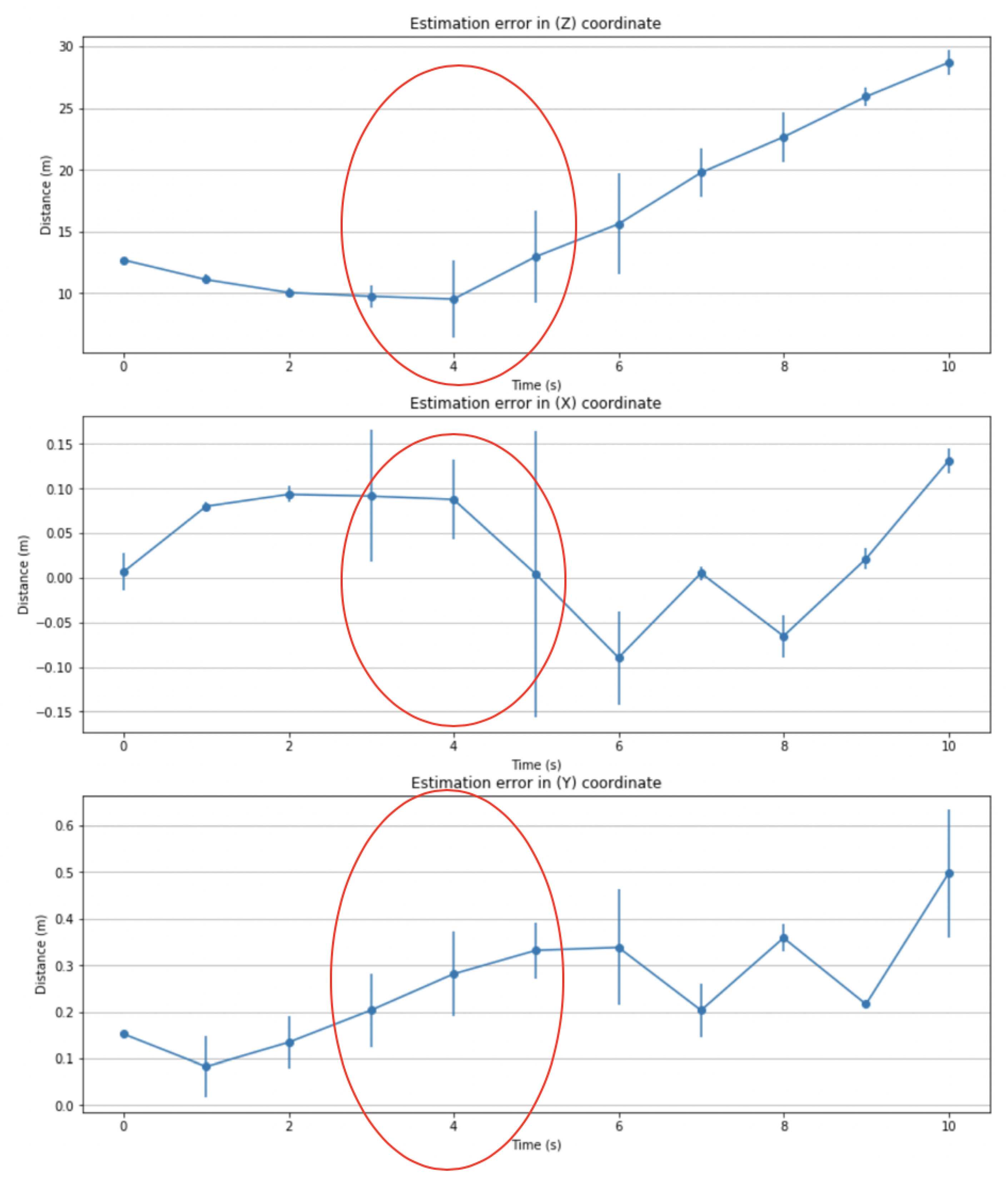
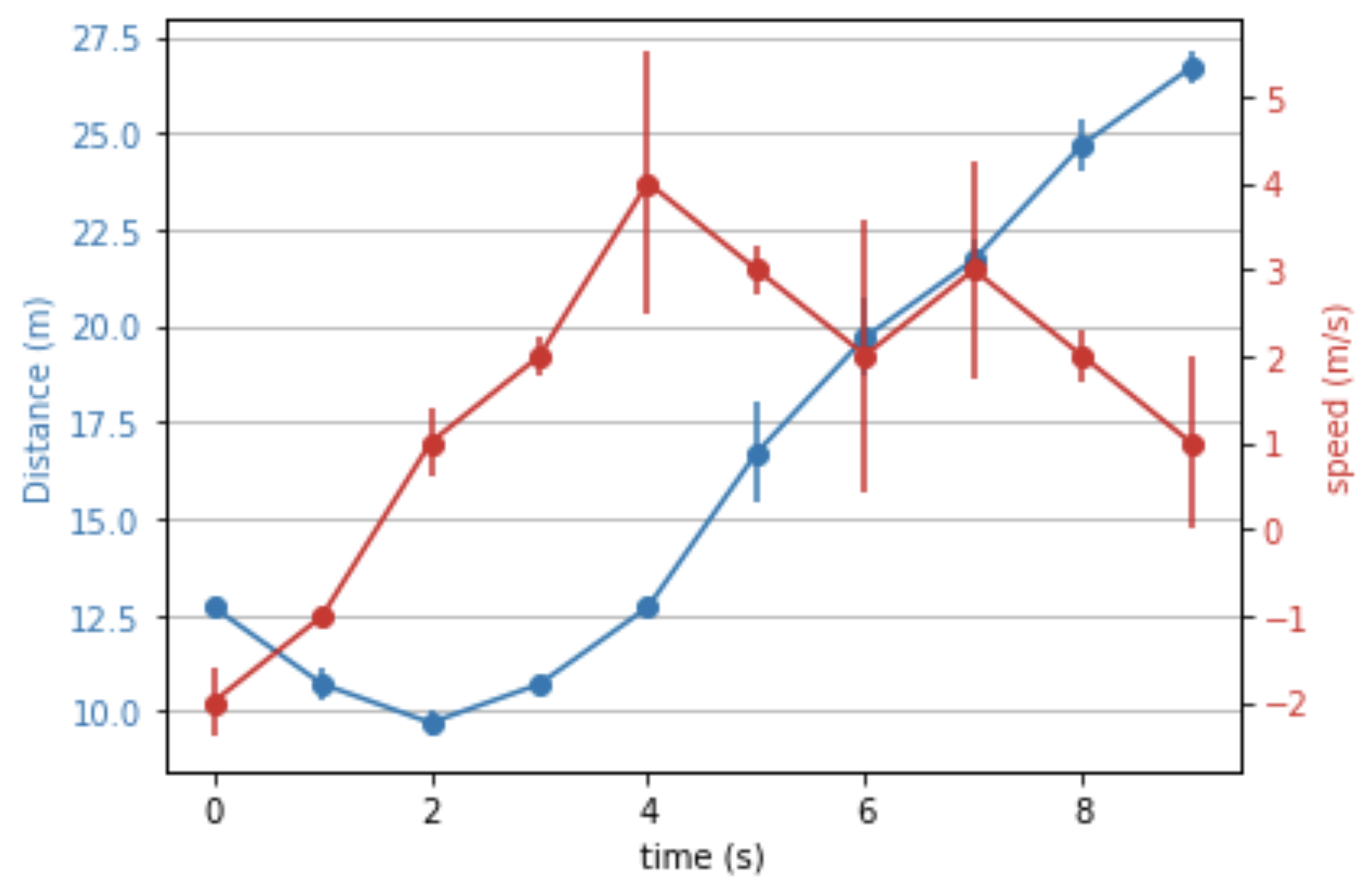
• This fusion allows the algorithm to work even in the case of full occlusion as shown in Figure 6. During occlusion, the estimation error grows. However, after the image comes back, the algorithm converges quickly;
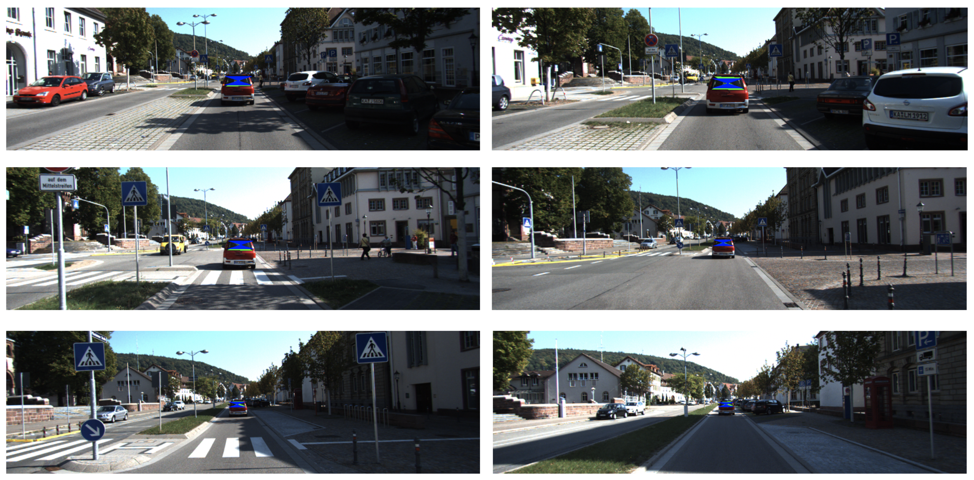
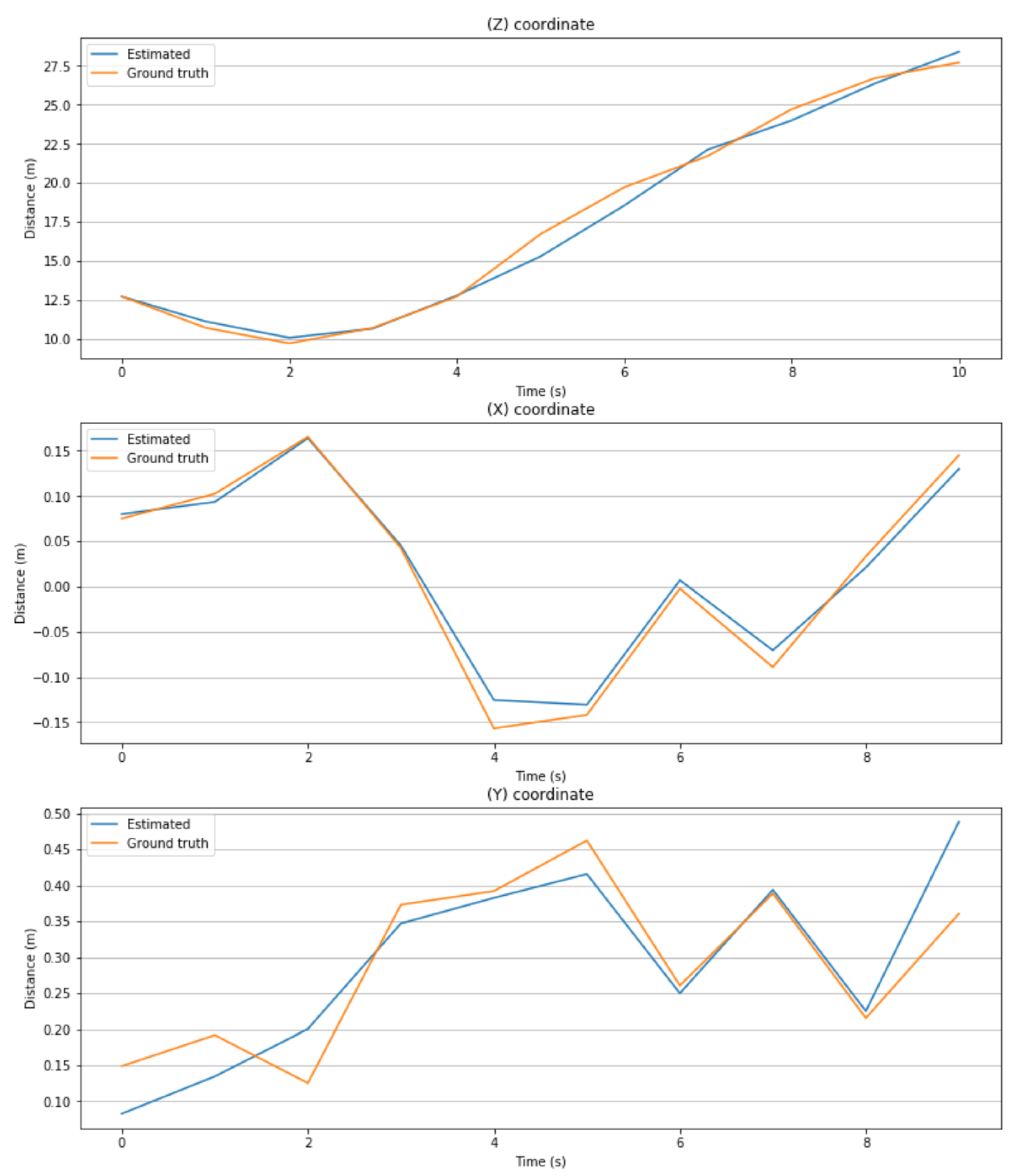
• In this paper, we used the Kitti dataset which has real driving scenarios. The results of the proposed algorithm are compared with the ground truth values obtained by the 2 cm accuracy 3D LiDAR to evaluate estimation error. Figure 4 presents the estimated 3D position using the proposed approach and its corresponding ground truth using the 3D LiDAR. Figure 5 and Figure 7 present estimation errors in 3D position and longitudinal velocity, respectively. These results show that the proposed approach can work in real driving scenarios;
• To the best of our knowledge, the existing works use 3D CAD models to estimate the position using one shot estimation [6,7,23]. The proposed approach has an advantage over the existing ones in the following aspects:

  -

  Other approaches do not take into account the dynamic motion constraints of the detected cars while the proposed approach fuses these motion constraints with semantic information to increase estimation accuracy;

  -

  Other approaches do not depend on temporal fusing. They depend on one shot estimation which does not work in the case of occlusion. In contrast, our approach depends on temporal fusing which allows it to predict car position and velocity in the case of occlusion;

  -

  Unlike other approaches which estimate the 3D position of a detected car only, the proposed approach estimates the velocity as well. Including car velocity in the state vector increases the accuracy of the estimation process due to the natural correlation between position and velocity of a detected car.

• A comparison between the proposed algorithm and the EPnP algorithm to estimate a detected car position using the KiTTi dataset is presented in Figure 8. The EPnP algorithm is one of the algorithms that depend on one shot estimation [23]. It estimates object position by minimizing the discrepancy between a virtual and a real image using the Levenberg–Marquardt method and is used in many other one-shot based algorithms [6]. From Figure 8, we can notice that the proposed approach slightly outperforms EPnP for distances up to 17 m. However, for distances greater than 17 m, the proposed approach has a better accuracy compared to EPnP algorithm. In addition, it is worth mentioning that EPnP, as well as other one shot-based approaches, will not work in the case of occlusion while the proposed approach can still predict the car position as presented in Figure 6;
• The experiments show that the algorithm can be used for short ranges and long ranges to get an idea of the traffic scene;
• According to Figure 9, the proposed algorithm is robust against different levels of measurement noise for distances up to 17 m. However, for distances greater than 17 m, the increase in measurements uncertainties will affect the estimation accuracy;
• The proposed algorithm depends on an object detection algorithm and a 3D CAD model matching algorithm to get a class ID and a matched 3D CAD model ID, respectively. In this paper, we assumed that the results of the object detection algorithm and the matching algorithm are correct. However, in real life, the results may be wrong. This introduces a limitation to the proposed approach as any errors in the class ID and/or the model ID will affect the estimation accuracy. It is possible to overcome this limitation by taking into account the uncertainties in class and model IDs during the estimation process. This can be done by augmenting the state vector to include, in addition to position and velocity variables, a class ID and a model ID and consider them as random variables to be estimated. The implementation of this point is out of the scope of the current paper and will be considered in future work;
• In this paper, Singer’s model (constant velocity model) was used to describe the dynamic motion of the detected car. This model is not enough to describe the motion in some cases, as it leads to incorrect results when the constant velocity condition is violated like in the case of turns. A more robust solution can be achieved by using Interacting Multiple Model filter (IMM filter) [25] where several motion models can be used to describe different types of motion scenarios. This point will be investigated in future work.

6. Conclusions

In this paper, we proposed an algorithm to estimate 3D position and velocity components of different cars in a scene. The algorithm fuses semantic information extracted from object detection algorithm with camera motion parameters measured by sensors on-board. The algorithm uses a prior known 3D CAD model to convert semantic information to metric information, which can be used in EKF. The experiments on the KiTTi dataset confirmed the proof of concept. It showed that the proposed algorithm works well and had an error of 3–5% at 30 m distance and a velocity estimation error up to 1 m/s. This percentage is small and allows the algorithm to produce a rough idea about the traffic scene at far distances. In addition, the results showed that the algorithm was able to converge quickly after a period of occlusion.

For future work, we plan to use the IMM filter to describe different motion models of the detected cars. In addition, more experiments with automated key points detection on several numbers of detected cars will be done to gain more insight into the performance of the proposed approach in different driving scenarios.

References

1. Cadena, C.; Carlone, L.; Carrillo, H.; Latif, Y.; Scaramuzza, D.; Neira, J.; Reid, I.; Leonard, J.J. Past, Present, and Future of Simultaneous Localization and Mapping: Toward the Robust-Perception Age. IEEE Trans. Robot. 2016, 32, 1309–1332. [Google Scholar] [CrossRef] [Green Version]
2. Mur-Artal, R.; Tardos, J. Probabilistic Semi-Dense Mapping from Highly Accurate Feature-Based Monocular SLAM. In Proceedings of the Robotics: Science and Systems XI, Sapienza University of Rome, Rome, Italy, 13–17 July 2015. [Google Scholar]
3. Campos, C.E.M.; Elvira, R.; Rodríguez, J.; Montiel, J.M.M.; Tardós, J.D. ORB-SLAM3: An Accurate Open-Source Library for Visual, Visual-Inertial and Multi-Map SLAM. arXiv 2020, arXiv:2007.11898. [Google Scholar]
4. Redmon, J.; Divvala, S.; Girshick, R.; Farhadi, A. You Only Look Once: Unified, Real-Time Object Detection. In Proceedings of the 2016 IEEE Conference on Computer Vision and Pattern Recognition (CVPR), Las Vegas, NV, USA, 27–30 June 2016; pp. 779–788. [Google Scholar]
5. Liu, W.; Anguelov, D.; Erhan, D.; Szegedy, C.; Reed, S.E.; Fu, C.; Berg, A.C. SSD: Single Shot MultiBox Detector. arXiv 2015, arXiv:1512.02325. [Google Scholar]
6. Chabot, F.; Chaouch, M.; Rabarisoa, J.; Teulière, C.; Chateau, T. Deep MANTA: A Coarse-to-fine Many-Task Network for joint 2D and 3D vehicle analysis from monocular image. arXiv 2017, arXiv:1703.07570. [Google Scholar]
7. Kundu, A.; Li, Y.; Rehg, J.M. 3D-RCNN: Instance-level 3D Object Reconstruction via Render-and-Compare. In Proceedings of the 2018 IEEE/CVF Conference on Computer Vision and Pattern Recognition (CVPR), Salt Lake City, UT, USA, 18–23 June 2018. [Google Scholar]
8. Wu, D.; Zhuang, Z.; Xiang, C.; Zou, W.; Li, X. 6D-VNet: End-To-End 6-DoF Vehicle Pose Estimation From Monocular RGB Images. In Proceedings of the IEEE/CVF Conference on Computer Vision and Pattern Recognition Workshops (CVPR), Long Beach, CA, USA, 16–17 June 2019. [Google Scholar]
9. Song, X.; Wang, P.; Zhou, D.; Zhu, R.; Guan, C.; Dai, Y.; Su, H.; Li, H.; Yang, R. ApolloCar3D: A Large 3D Car Instance Understanding Benchmark for Autonomous Driving. arXiv 2018, arXiv:1811.12222. [Google Scholar]
10. Manhardt, F.; Kehl, W.; Gaidon, A. ROI-10D: Monocular Lifting of 2D Detection to 6D Pose and Metric Shape. arXiv 2018, arXiv:1812.02781. [Google Scholar]
11. He, T.; Soatto, S. Mono3D++: Monocular 3D Vehicle Detection with Two-Scale 3D Hypotheses and Task Priors. arXiv 2019, arXiv:1901.03446. [Google Scholar] [CrossRef]
12. Qin, Z.; Wang, J.; Lu, Y. MonoGRNet: A Geometric Reasoning Network for Monocular 3D Object Localization. arXiv 2018, arXiv:1811.10247. [Google Scholar] [CrossRef]
13. Barabanau, I.; Artemov, A.; Burnaev, E.; Murashkin, V. Monocular 3D Object Detection via Geometric Reasoning on Keypoints. arXiv 2019, arXiv:1905.05618. [Google Scholar]
14. Ansari, J.A.; Sharma, S.; Majumdar, A.; Murthy, J.K.; Krishna, K.M. The Earth ain’t Flat: Monocular Reconstruction of Vehicles on Steep and Graded Roads from a Moving Camera. arXiv 2018, arXiv:1803.02057. [Google Scholar]
15. Girshick, R.; Donahue, J.; Darrell, T.; Malik, J. Rich feature hierarchies for accurate object detection and semantic segmentation. arXiv 2013, arXiv:1311.2524. [Google Scholar]
16. Girshick, R. Fast R-CNN. In Proceedings of the 2015 IEEE International Conference on Computer Vision (ICCV), Santiago, Chile, 7–13 December 2015; pp. 1440–1448. [Google Scholar]
17. Ren, S.; He, K.; Girshick, R.B.; Sun, J. Faster R-CNN: Towards Real-Time Object Detection with Region Proposal Networks. arXiv 2015, arXiv:1506.01497. [Google Scholar] [CrossRef] [PubMed] [Green Version]
18. Redmon, J.; Farhadi, A. YOLOv3: An Incremental Improvement. arXiv 2018, arXiv:1804.02767. [Google Scholar]
19. Bowman, S.L.; Atanasov, N.; Daniilidis, K.; Pappas, G.J. Probabilistic data association for semantic SLAM. In Proceedings of the 2017 IEEE International Conference on Robotics and Automation (ICRA), Singapore, 29 May–3 June 2017; pp. 1722–1729. [Google Scholar]
20. Doherty, K.; Fourie, D.; Leonard, J. Multimodal Semantic SLAM with Probabilistic Data Association. In Proceedings of the 2019 International Conference on Robotics and Automation (ICRA), Montreal, QC, Canada, 20–24 May 2019; pp. 2419–2425. [Google Scholar]
21. Doherty, K.; Baxter, D.; Schneeweiss, E.; Leonard, J.J. Probabilistic Data Association via Mixture Models for Robust Semantic SLAM. arXiv 2019, arXiv:1909.11213. [Google Scholar]
22. Davison, A.J. FutureMapping: The Computational Structure of Spatial AI Systems. arXiv 2018, arXiv:1803.11288. [Google Scholar]
23. Lepetit, V.; Moreno-Noguer, F.; Fua, P. EPnP: An accurate O(n) solution to the PnP problem. Int. J. Comput. Vis. 2009, 81. [Google Scholar] [CrossRef] [Green Version]
24. Singer, R.A. Estimating Optimal Tracking Filter Performance for Manned Maneuvering Targets. IEEE Trans. Aerosp. Electron. Syst. 1970, AES-6, 473–483. [Google Scholar] [CrossRef]
25. Bar-Shalom, Y.; Li, X.; Kirubarajan, T. Estimation with Applications to Tracking and Navigation: Theory, Algorithms and Software; John Wiley & Sons Ltd.: Chichester, UK, 2001. [Google Scholar]
26. Stepanov, O.A. Optimal and Sub-Optimal Filtering in Integrated Navigation Systems. In Aerospace Navigation Systems; Nebylov, A., Watson, J., Eds.; John Wiley & Sons Ltd.: Chichester, UK, 2016; pp. 244–298. [Google Scholar]
27. Sabattini, L.; Levratti, A.; Venturi, F.; Amplo, E.; Fantuzzi, C.; Secchi, C. Experimental comparison of 3D vision sensors for mobile robot localization for industrial application: Stereo-camera and RGB-D sensor. In Proceedings of the 2012 12th International Conference on Control Automation Robotics & Vision (ICARCV), Guangzhou, China, 5–7 December 2012; pp. 823–828. [Google Scholar]
28. Geiger, A.; Lenz, P.; Urtasun, R. Are we ready for Autonomous Driving? The KITTI Vision Benchmark Suite. In Proceedings of the Conference on Computer Vision and Pattern Recognition (CVPR), Providence, RI, USA, 16–21 June 2012. [Google Scholar]
29. Multi-Object Tracking Benchmark. The KITTI Vision Benchmark Suite. Available online: http://www.cvlibs.net/datasets/kitti/eval_tracking.php (accessed on 10 August 2020).
30. OXTS. RT v2 GNSS-Aided Inertial Measurement Systems; Revision 180221; Oxford Technical Solutions Limited: Oxfordshire, UK, 2015. [Google Scholar]
31. Mansour, M.; Davidson, P.; Stepanov, O.; Raunio, J.P.; Aref, M.M.; Piché, R. Depth estimation with ego-motion assisted monocular camera. Gyroscopy Navig. 2019, 10, 111–123. [Google Scholar] [CrossRef]
32. Davidson, P.; Mansour, M.; Stepanvo, O.; Piché, R. Depth estimation from motion parallax: Experimental evaluation. In Proceedings of the 26th Saint Petersburg International Conference on Integrated Navigation Systems (ICINS), Saint Petersburg, Russia, 27–29 May 2019. [Google Scholar]
33. Mansour, M.; Davidson, P.; Stepanov, O.; Piché, R. Relative Importance of Binocular Disparity and Motion Parallax for Depth Estimation: A Computer Vision Approach. Remote Sens. 2019, 11, 1990. [Google Scholar] [CrossRef] [Green Version]
Figure 1. The algorithm pipeline focusing on an ego lane car. It is divided into two parts: Extracting the semantic information (in red) and temporal fusing (in blue). (1) The car is detected in the scene using an object detection algorithm like Yolov3. (2) The key points of the car are extracted and matched against several 3D CAD models to select the corresponding model [6,7,8]. (3) The extracted semantic information is converted to 3D coordinates using the 3D CAD model. (4) The car position is predicted using the ego motion parameters of the camera. (5) Virtual 2D key points are created using the predicted car position and the 3D coordinates of the key points obtained from the CAD model. (6) The distance between actual 2D key points and their corresponding 2D virtual key points is computed. (7) The filter is updated using the computed discrepancy.
Remotesensing 13 00388 g001
Figure 2. The used coordinate systems for the camera (in black) and the detected car (in blue).
Remotesensing 13 00388 g002
Figure 3. The results of the algorithm pipeline focusing on an ego lane car. The estimated 3D position of the rear windshield corners (in blue) are superimposed on the image against the ground truth position (in green).
Remotesensing 13 00388 g003
Figure 4. The estimated 3D coordinates of the detected car using the proposed algorithm.
Remotesensing 13 00388 g004
Figure 5. Estimation error in the car position presented as error bars around the estimated value.
Remotesensing 13 00388 g005
Figure 6. Estimation error in car coordinates in the case of occlusion. The period of occlusion is highlighted with a red oval.
Remotesensing 13 00388 g006
Figure 7. Estimation error in P z c a r and the longitudinal velocity V z c a r .
Remotesensing 13 00388 g007
Figure 8. Distance estimation using the proposed algorithm and EPnP algorithm [23].
Remotesensing 13 00388 g008
Figure 9. Distance estimation with different levels of image point noise.
Remotesensing 13 00388 g009
Publisher’s Note: MDPI stays neutral with regard to jurisdictional claims in published maps and institutional affiliations.