Article

Spatiotemporal Characteristics and Trend Analysis of Two Evapotranspiration-Based Drought Products and Their Mechanisms in Sub-Saharan Africa

1
Binjiang College, Nanjing University of Information Science & Technology, No.333 Xishan Road, Wuxi 214105, China
2
Collaborative Innovation Center on Forecast and Evaluation of Meteorological Disasters, School of Geographical Sciences, Nanjing University of Information Science & Technology, Nanjing 210044, China
3
Jiangsu Meteorological Bureau, Meteorological Services Center, Nanjing 210008, China
4
School of Geosciences, Department of Geographic Sciences, University of Energy and Natural Resources, P.O. Box 214 Sunyani, Ghana
5
College of Atmospheric Sciences, Nanjing University of Information Science and Technology, Nanjing 210044, China
6
Key Lab of Northwest Water Resources, Environment and Ecology, School of Environmental and Municipal Engineering, Xi’an University of Architecture and Technology, No.13 Yanta Road, Xi’an 710055, China
*
Author to whom correspondence should be addressed.
Submission received: 23 December 2020 / Revised: 23 January 2021 / Accepted: 29 January 2021 / Published: 2 February 2021
(This article belongs to the Special Issue Satellite Remote Sensing for Tropical Meteorology and Climatology)

Abstract

:
Drought severity still remains a serious concern across Sub-Saharan Africa (SSA) due to its destructive impact on multiple sectors of society. In this study, the interannual variability and trends in the changes of the self-calibrating Palmer Drought Severity Index (scPDSI) based on the Penman–Monteith (scPDSIPM) and Thornthwaite (scPDSITH) methods for measuring potential evapotranspiration (PET), precipitation (P), normalized difference vegetation index (NDVI), and sea surface temperature (SST) anomalies were investigated through statistical analysis of modeled and remote sensing data. It was shown that scPDSIPM and scPDSITH differed in the representation of drought characteristics over SSA. The regional trend magnitudes of scPDSI in SSA were 0.69 (scPDSIPM) and 0.2 mm/decade (scPDSITH), with a difference in values attributed to the choice of PET measuring method used. The scPDSI and remotely sensed-based anomalies of P and NDVI showed wetting and drying trends over the period 1980–2012 with coefficients of trend magnitudes of 0.12 mm/decade (0.002 mm/decade). The trend analysis showed increased drought events in the semi-arid and arid regions of SSA over the same period. A correlation analysis revealed a strong relationship between the choice of PET measuring method and both P and NDVI anomalies for monsoon and pre-monsoon seasons. The correlation analysis of the choice of PET measuring method with SST anomalies indicated significant positive and negative relationships. This study has demonstrated the applicability of multiple data sources for drought assessment and provides useful information for regional drought predictability and mitigation strategies.

Graphical Abstract

1. Introduction

According to the fifth assessment report (AR5) of the Intergovernmental Panel on Climate Change (IPCC), global warming has significantly contributed to the evolution of extreme weather events (such as droughts, floods, and heat waves) [1]. The increase in the severity of these weather events has been documented due to their devastating impact on our ecosystem and different sectors of society [2]. The projected increase in potential future drought events as a result of current global warming has been of keen interest to scholars, researchers, and the general public [1].
Generally, to depict and monitor drought events, specialized drought indices are used. However, one key question of concern has been about the proxies used to measure these droughts. For instance, some studies have questioned the use of precipitation (P) deficits as a primary method of depicting historical droughts in a warming climate [3,4,5,6], particularly when there is ample evidence of enhanced atmospheric demand under recent global warming. A decrease in P is generally associated with increased temperature (T) (and reduced atmospheric humidity), which enhances potential evapotranspiration (PET) and later intensifies dry spells [4,5,6]. Therefore, using or including atmospheric water demand (or PET) in the depiction of drought events is worthwhile. A review by Mishra and Singh [7] outlined a lengthy catalog consisting of multiple specialized drought indices, highlighting both the concept of atmospheric “supply” and “demand” and how they account for the surface warming effect on wet and dry spells.
Although there is a lack of general consensus on global drought assessments [8,9,10,11,12], drought indices designed on the basis of the concept of atmospheric supply and demand have shaped our understanding of drought [3,7,13,14,15]. Thus, within this context, the self-calibrating Palmer Drought Severity Index (scPDSI), a typical example of such a drought index [12], has been widely used for drought climatology studies at global scales [8,9] and for regional specific studies [15,16,17,18,19], among others [6]. The scPDSI, by design, is a physical-based drought index that incorporates antecedent P, moisture supply, and demand (i.e., potential evaporation (PET)) to account for surface warming effects on wet and dry spells [12].
Several studies have reported intense drying and increased frequency of droughts in many regions around the world [7]. However, controversy remains in the order of magnitude of dry spells and changes (or trends) in drought severity, although there are several reasons for this lack of agreement. The choice of PET used remains the most prominent issue. PET computation (a proxy for atmospheric demand) is sensitive to the choice of PET method used [12,20,21]. The different methods of PET estimation are outlined in Mishra and Singh [7]. Here, we focus on only the Thornthwaite and Penman–Monteith methods. In most studies, the Thornthwaite method has been shown to overestimate drying trends more than the Penman–Monteith method and vice-versa [12,20,21]. Nonetheless, the accuracy and rationality of the two PET methods and their application are still under study [6,7,12].
In this study, we attempt to understand the impact of the two PET methods on drought characteristics and trends in the large-scale convective region of Sub-Saharan Africa (SSA) (i.e., a region explored in few studies) [22,23]. In addition, our study uses remotely sensed precipitation (P) and vegetation datasets to investigate how these climate variables respond to drought trends in SSA. Furthermore, we explore the interactive effects of sea surface temperature (i.e., El Niño–Southern Oscillation (ENSO) and Indian Ocean Dipole (IOD)) on drought trends, a study initiative that is lacking and has been recommended [22].
Agriculture is the backbone of the overall economic growth of SSA countries. Agriculture not only contributes to nearly 24–31% of the gross domestic product (GDP) of SSA countries, but is also essential for poverty reduction and food security, as it employs more than 65% of the workforce [24]. Apart from other constraints to agricultural development in Africa, the SSA agricultural system is vulnerable to patterns and mechanisms of climate change [24]. The spatio-temporal variability of P, coupled with high population growth, amplifies the region’s vulnerability to droughts due to increasing water demand [23]. Agriculture plays a role in reducing poverty in the region, hence the launch of the Malabo Goals 2025 and the 2030 Agenda for Sustainable Development and Sustainable Development Goal 2 (SDG2) [24].
To the best of our knowledge, few attempts have been made in SSA to compare long-term drought characteristics and trends using energy-driven drought indices [22,23]. Thus, in a warming climate, a better understanding of drought characteristics, trends, and mechanisms influencing SSA is useful within the context of regional predictability and mitigation strategies. This study highlights a number of controlling factors that may potentially impact drought characteristics in diverse climate regions of SSA. Moreover, the high growth in population and environmental degradation, especially in arid and semi-arid regions, has caused many major rivers and their tributaries to dry up. For example, the upstream of river basins such as the Volta, Nile, Niger, and Zambezi has experienced a high intensity of water resource utilization over the last three decades [1,2,24]. Thus, in this paper, we seek to contribute to the existing literature on droughts in the region by using state-of-the-art modeled data and satellite products in a region where data availability and quality concerns remain a challenge. Our main objective is to analyze drought characteristics and the interannual drought patterns and to determine the relationship between drought and control factors such as P, vegetation, and teleconnection indices. First, we used long-term modeled scPDSI based on two PET methods to determine significant spatial patterns of annual drought characteristics (in terms of their frequency, spatial extent, and intensity). Second, we used the Mann–Kendall and Sen’s slope methods to analyze temporal variability of times corresponding to the significant patterns for modeled data and satellite products. Next, we investigated the relationships between the time variability of significant patterns and (1) hydroclimate factors (e.g., P), (2) vegetation, and (3) teleconnection indices across SSA.
The paper is organized as follows. In Section 2, we provide a brief description of the different data used. We also summarize the methods and approaches used in this section. The results of the comparison are presented in Section 3. Section 4 is a discussion of the most important study findings, and Section 5 concludes.

2. Materials and Methods
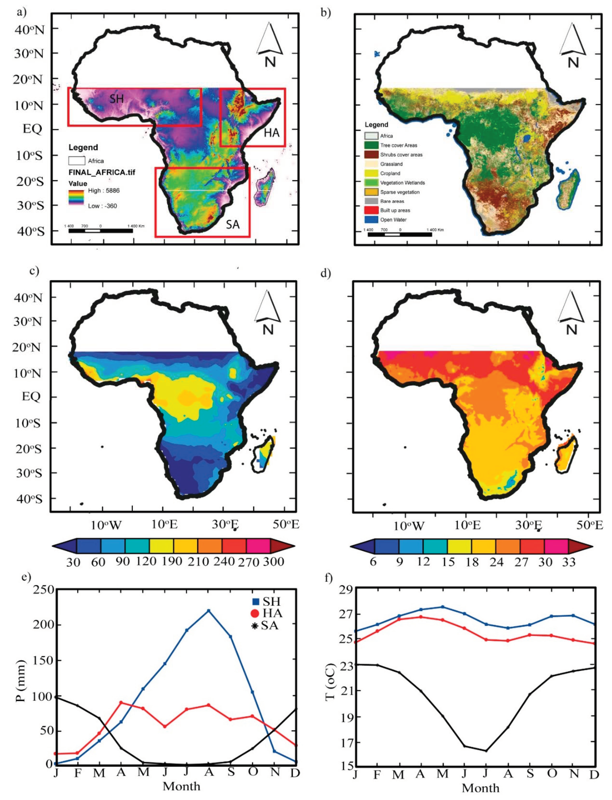
2.1. Study Area

Sub-Saharan Africa (SSA) is defined as the vast land mass area south of the Sahara Desert between 15°0′0″N and 35°0′0″S and between 14°0′0″W and 52°0′0″E. SSA is bordered to the southeast by the Indian Ocean and to the west by the Atlantic Ocean (Figure 1). It has a total area of nearly 24.7 million km2 (accounting for approximately 81.2% of the entire African land area). The region straddles the equator with a significant number of countries located in both the Northern and Southern Hemispheres.
Generally, the topography, the vegetation conditions, the oscillation of the intertropical convergence zone (ITCZ), and the atmospheric processes impact precipitation (P) variability throughout the hydrological system [25,26]. The elevation of SSA ranges from −360 to 5861 m above mean sea level (msl), with the highlands located in the eastern and southern parts of the region (Figure 1a).
The weather pattern shows two clear seasons (the wet and dry seasons) with a wide range of climatic features [27]. The tropical wet and dry climate located along the Guinean coast and the equatorial region have an elevation <850 m above msl. The Savanna climate covers nearly three quarters of SSA land mass, with elevation ranging from >170 to <5861 m above msl. The semi-arid climates are found in the Sudano-Sahelian, large parts of Southern Africa, and the Horn of Africa, which have elevation ranges from >250 to <5000 m. Arid climates are found in most parts of Southern Africa and the Horn of Africa, with elevation ranges from >780 to <5861 m.
The complexity of the topographical features partly explains the high seasonal and interannual variability in P. Figure 1c,d present the annual mean and seasonal climatology of precipitation (P) and temperature (T) over the period 1981 to 2017.
Based on the Climate Hazard Group Infrared Precipitation with Stations (CHIRPS) dataset, the annual mean P in SSA ranges from <30 to >300 mm. We observed in Figure 1c that areas with high elevation (i.e., the Ethiopian highlands) or dense vegetation (i.e., the Guinean coast and Congo’s forested areas) receive an annual mean P > 150 mm. The Savanna and Sudano-Sahelian belt climate regions receive <120 and <90 mm, respectively. Arid regions receive an annual mean P as low as <30 mm.
However, based on the European Center for Medium-Range Weather Forecasts (ECMWF) ERA-5 atmospheric reanalysis datasets, the arid climate regions in Southern Africa have annual mean T ranges from 15 to <27 °C. The semi-arid climate ranges from 24 to >33 °C. The tropical wet and dry climate records indicate <27 °C (Figure 1d).
The P and T pattern in the northern part of SSA is generally bimodal (Figure 1e,f). In this region, we observe that the P and T seasonality is not synchronous (Figure 1e,f, blue and red), as an increase in P from June to August (JJA) and September to November (SON) leads to a decrease in T. These seasonal characteristics coupled with other factors (explained below) define the region’s monsoon climate.
For example, the Western Africa region receives long rains in boreal summer (i.e., June to August (JJA)) and short rains in boreal autumn (September to November (SON)), with peak values in August (Figure 1e, blue). The Horn of Africa (HoA) region receives mostly long P in boreal spring (i.e., March to May (MAM)) and short P from October to December (OND) (Figure 1c, red). However, the southern parts of SSA have a unimodal P and T pattern (Figure 1e,f, black), with long rains in austral summer (i.e., December–February (DJF).
Under the recent warming climate, changes in P and T over space and time are partly induced by local factors such as the heterogeneity of the land surface. According to the 2016 land use land cover (LULC) map from the European Space Agency Climate Change Initiative (ESACCI) [28], grassland and cropland occupy 17% and 12%, mainly along the Sudano-Sahelian belt–Guinea coast (SSG), Horn of Africa (HoA), the peripherals of large open water bodies, and the Eastern Southern Africa regions (Figure 1b). Dense vegetation accounts for nearly 21% and is distributed along the Guinean coast, the Congo basin, and the equatorial forests regions. Shrubland (covering 11%) is located mainly in the Horn of Africa region and the Southern Central Africa regions. Bare land occupies 32% of the land area and is located mainly in the Sahara Desert (masked out) and parts of the Southern Africa area. Open water bodies (covering 7.2%) are interspersed and distributed mainly in the equatorial regions and south of the equator. The remaining cover types (covering 1.4%) such as sparse vegetation, vegetated wetland, and buildup areas are interspersed across SSA (Table 1).
Precipitation (P) variability is partly impacted by the interaction with global climate forcing systems, such as the El Niño–Southern Oscillation (ENSO) and the Indian Ocean Dipole (IOD). These teleconnections in space and time are widely reported to explain the annual and seasonal P variability in SSA [29,30].
To examine specific drought characteristics and trends in detail, three regions were selected (see Figure 1a). The boxes in Figure 1a indicate the three sub-regions used for the spatial averaged analysis: the Sudano-Sahelian–Guinean Coast (SSG) (5°N–15°N, 5°W–20°E), the Horn of Africa (HoA) (5°S–15°N, 30°–52°E), and the Southern Africa region (SAR) (32°S–15°S, 8°–32°E).
The SSG region used in this paper includes the Sahelian belt, the Sudanian belt, and parts of the Guinean coast stretching from the Atlantic Ocean to the central region at longitudes of 20°E. The HoA used here extends from the interior of the Ethiopian and Kenyan highlands to the coast of the Indian Ocean. The SAR includes areas that lie below 15°S. The justification for selecting the limits of the boxes was based on their interannual P variations, the mean climate, and the associations with teleconnections [29,30,31,32].

2.2. Data Description

Here we briefly describe the specific data sets used in this study.

2.2.1. Drought Index Data

We used a self-calibrated Palmer Drought Severity Index (scPDSI) [34] to characterize drought events in SSA. The scPDSI has been recommended as a good proxy for surface soil moisture conditions and for drought monitoring [7]. In the design of the PDSI, several climatic variables were incorporated to reflect the drying and wetting conditions of an area. Thus, to characterize drought events, we used PDSI datasets downloaded from the Princeton website [35].
The PDSI dataset has a global coverage at a 1° × 1° spatial resolution and a monthly temporal resolution (over the period 1948–2008) [9,36]. Sheffield et al. [36] developed two kinds of PDSI based on the Thornthwaite and the Penman–Monteith algorithms. The climate forcing datasets (i.e., covering 1979–2008) used to produce this scPDSI reflected and captured all forms of anthropogenic activities in the region. Particularly, within the context of global warming, SSA has experienced several years of land use land cover (LULC). The dataset is publicly available, and readers may refer to the developers [9,36] for detailed information on accuracy, the rationality of the input forcing data, the choice of baseline period, and calculation schemes.

2.2.2. Satellite-Based Normalized Difference Vegetation Index (NDVI)

To study the spatio-temporal patterns of vegetation greenness and their responses to drying and wetting conditions, we used the Normalized Difference Vegetation Index (NDVI) from the Global Inventory Modeling and Mapping Studies (GIMMS) NDVI3g dataset product with a temporal resolution of 15-day intervals and a 1/12-degree spatial resolution, processed and archived by the GIMMS group at NASA [37]. The NDVI used in this study spans from 1982 to the present. To ensure the robustness of long-term trends and variability, the GIMMS group corrected and calibrated the dataset to minimize sensor effects by using high quality NDVI data from state-of-the-art sensors and retrieval algorithms (i.e., Bayesian methods). The algorithm for calculating NDVI is presented in Equation (1).
NDVI = NIR VIS NIR + VIS
where NIR and VIS denote near-infrared and red (visible) top-of-atmosphere reflectance, respectively.
Generally, NDVI ranges from +1 to −1. However, for this study, only vegetated areas were considered from the range of 0.2–0.8 pixels, while pixel values <0.12 were masked out to ensure that only NDVI values related to vegetation greenness were captured, following Martiny et al. [38]. This means that bare soils and desert areas that corresponded to mean pixel values <0.12 and negative values were excluded. For more details on GIMMS NDVI3g dataset products, readers are referred to the following [37].

2.2.3. Climate Hazard Group Infrared Precipitation with Stations (CHIRPS)

We selected CHIRPS products that produce gridded monthly P products from combined in-situ and satellite inputs for monitoring extreme events such as floods, droughts, or heat waves [37]. CHIRPS is a semi-global precipitation product and is publicly available at the Climate Hazards Group [39] and the International Research Institute climate data library [40] at several temporal resolutions and at a 0.05° spatial resolution.
However, we chose the second version of CHIRPS (1981–present) with a spatial resolution of 0.05° ranging from 50°S to 50°N (and all longitudes) at a monthly temporal resolution [39,41]. The production of CHIRPS was explained by Funk et al. [39]. CHIRPS is widely used for various applications [42,43].

2.2.4. Sea Surface Temperature (SST) Indices

In order to study and explain the effect of teleconnections on drought evolution, we downloaded the Indian Ocean Dipole (IOD) and the Ni-no-3.4 (N3.4) sea surface temperature (SST) indices from their respective websites [44,45]. Our study chose a monthly time step for the period from January 1979 to December 2012 to provide a general picture of the relationship between both IOD and El Niño–Southern Oscillation (ENSO) and drought trends over the region. Ni-no-3.4 (N3.4) originates from the Climate Prediction Center (CPC) over the 5°N–5°S, 170°–120°W regions. Smith et al. [46] have provided comprehensive documentation and computation for these datasets.

2.2.5. Other Auxiliary Datasets

To represent the temperature (T) climatology of the region, we acquired gridded monthly ERA-5 T data aggregated at 0.25 × 0.25° resolution. The ERA-5 T dataset is a global atmospheric reanalysis product produced by ECMWF [47]. In addition, we used a 20 m resolution LULC map acquired from the ESACCI [28] and a 30 m Shuttle Radar Topography Mission (SRTM) digital elevation map (DEM) downloaded from the NASA (SRTM) website [33] to visualize the LULC and elevation of the region.

2.3. Methods

2.3.1. Data Preprocessing

Our first step was to pre-process the drought dataset used in this study. For simplicity of presentation, we used scPDSIPM and scPDSITH to represent the PDSI index based on the Penman–Monteith and Thornthwaite methods, respectively.
From the global PDSI dataset, the first preprocessing task was to constrain the scPDSI values to a range from −10 to 10 (based on Dai et al. [12]), prior to masking the study area. In order to measure a drought event, we needed to define a drought threshold. Based on the literature on the scPDSI range (see Table 2), we defined drought events [8,16]. Table 2 provides a classical Palmer [46] classification for wet and dry conditions. Thus, using scPDSI time series per grid, we identified for each grid scPDSI values below some user-defined thresholds. We used a threshold of −2.0 to denote moderate drought events and −4.0 for more extreme droughts.
In addition, we aggregated the biweekly NDVI data into monthly values and then aggregated those into annual and seasonal values over the period 1982–2012 by simple spatial and temporal averages. Moreover, CHIRPS P grid points covering SSA were extracted and aggregated from monthly to annual and seasonal averages for each year. Lastly, we re-gridded all the satellite (i.e., CHIRPS P and NDVI) datasets to match the scPDSI dataset resolution using nearest neighbor [48,49].

2.3.2. Statistical Analysis

Analyses in this study were based on annual and seasonal changes. Different statistical methods were used to compare and analyze the differences among the datasets. For seasonal analysis, we adopted pre-monsoon and monsoon seasons. Thus, we calculated the seasonal mean of the monthly time series (for each pixel) for pre-monsoon (November–March (NDJFMA)) and monsoon (May–September (MJJASO)) seasons to capture the boreal and austral P regimes in both areas in the northern and southern part of SSA, NH and SH, respectively.
Moreover, in the annual time step, we calculated the spatial mean for each year for each pixel. For interannual analysis, the main statistical parameters used in the temporal analysis were means over the period. Next, drought trends and temporal changes per grid over the period were performed using the Mann–Kendall non-parametric statistical test (M-K) [50,51] and Sen’s slope estimator [52] at a 0.05 significance level based on the World Meteorological Organization (WMO) recommendations, widely followed to assess trends in climatological and hydrological time series [53,54].
To apply the statistical tests, we defined two (i.e., the null and alternative) hypotheses for the scPDSI, CHIRPS, and NDVI datasets as follows:
  • H0 = null hypothesis of trend absence in time series;
  • H1 = alternative hypothesis of trend in time series.
The detailed theory and estimation procedure for both the M–K and Sen’s slope estimator are presented in [53].
In addition, in analyzing the interannual variability, the P and NDVI anomalies were calculated based on the spatially averaged annual and seasonal values of each pixel. Negative P and NDVI values denote drying and vegetative stress, and positive values denote wetting trends and vegetation greening. We also conducted two kinds of correlation analysis to precisely examine and understand the effects of climatic factors (i.e., P), vegetation conditions (i.e., NDVI), and teleconnections indices (i.e., ENSO and IOD) on wet and dry spells. We computed spatial correlation to analyze their spatial dynamics on scPDSI, while for temporal correlation, we conducted a pixel-wise correlation of each variable on an annual and seasonal scales to understand the temporal dynamics. All relationships were calculated for the period 1982–2012.

3. Results

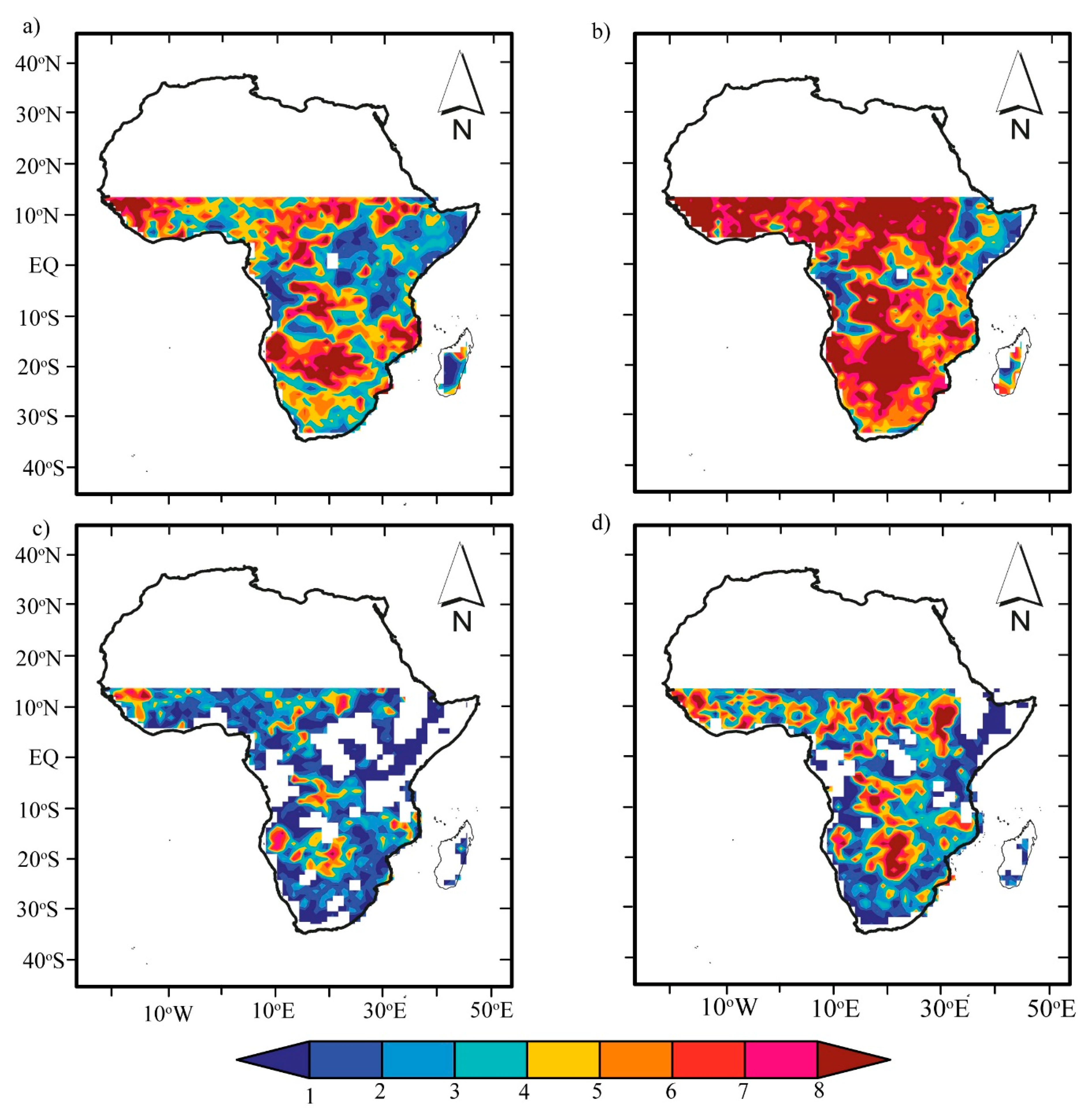
3.1. Spatiotemporal Characteristics of Sub-Saharan Africa (SSA) Droughts

The comparison between the characteristics of the two drought datasets (scPDSIPM and scPDSITH) was explored to determine how the two datasets represent droughts over the SSA. Figure 2 presents the spatial pattern of the drought frequencies of two scPDSI datasets across SSA over the period 1979–2012. Figure 2a,b show frequencies for moderate drought, while Figure 2c,d present frequencies for extreme drought. Overall, both scPDSI datasets differed in representing drought frequencies over space. Particularly, areas located in the northwest tips of the SSG, patches north and south of the Congo basin, and patches surrounding the Kalahari Desert to the southeast tip of Mozambique (on 18°S–22°S) showed similar agreement in detecting moderate and extreme droughts. However, moderate (extreme) drought occurred more (less) frequently and affected larger (smaller) areas in scPDSITH relative to scPDSIPM (Figure 2a,d). However, disagreement was found between the two scPDSI datasets in a few areas, characterized by complex topography, large water bodies/wetlands, and dense vegetation.
To analyze the drought intensity over the same across the SSA, the annual mean intensity was computed. Figure 3 shows maps of the mean annual drought intensity between the moderate (top panel) and extreme (bottom panel) drought events for both scPDSI datasets. However, scPDSITH shows more intensification and a larger affected area than scPDSIPM. Figure 3a,b present spatial intensity for moderate droughts with a similar spatial pattern and magnitude, as in Figure 2a,b. The results show that locations with high (low) intensities but extreme droughts are more intensified in scPDSITH relative to scPDSIPM (Figure 2c,d).
To understand the trends and temporal changes in drought intensities for each grid, regional trends in drought intensity for SSA and three selected regions (see Figure 1a) were investigated, and the results are shown in Figure 4. The interannual variations in moderate drought for both scPDSI datasets show an increased trend in the whole SSA, the SSG, and the Southern Africa region (SAR) (Figure 4a–c, respectively). In contrast, only the HoA exhibited stationarity in drought intensity, but extreme drought intensified over the period 1979–2012.
The relationships between drought and frequency, areal extent, and intensity over SSA from 1979–2012 were analyzed (Figure 5). Figure 5a,b show the interannual variation in frequency and areas affected (shown in bar graphs) for moderate (Figure 5a) and extreme (Figure 5b) droughts. In all, the frequency and area affected (in km) varied considerably, where more (less) frequent droughts affected larger (smaller) land area (Figure 5a,b).
Comparatively, in the mid-1980s, 1990s, and 2000s, more areas were significantly affected by moderate droughts than by extreme droughts. However, the drought-affected area in scPDSIPM decreased after 1995, while that in scPDSITH increased.
Next, the relationships between drought intensity and frequency were compared (Figure 5a,d). The temporal changes in drought intensity show opposite trends relative to frequency in both datasets (Figure 5a,d). Moderate drought shows more intensification than extreme droughts from 1995 onwards (Figure 5c,d). However, similar to the interannual variations in frequency, there is considerable disagreement in the interannual variations between the scPDSI datasets, especially after 1995. Similarly, more (less) frequent droughts have low (high) intensity. Thus, our results are consistent with previous regional studies, where the Thornthwaite method is reported to exaggerate drought frequency and intensity [8,55].

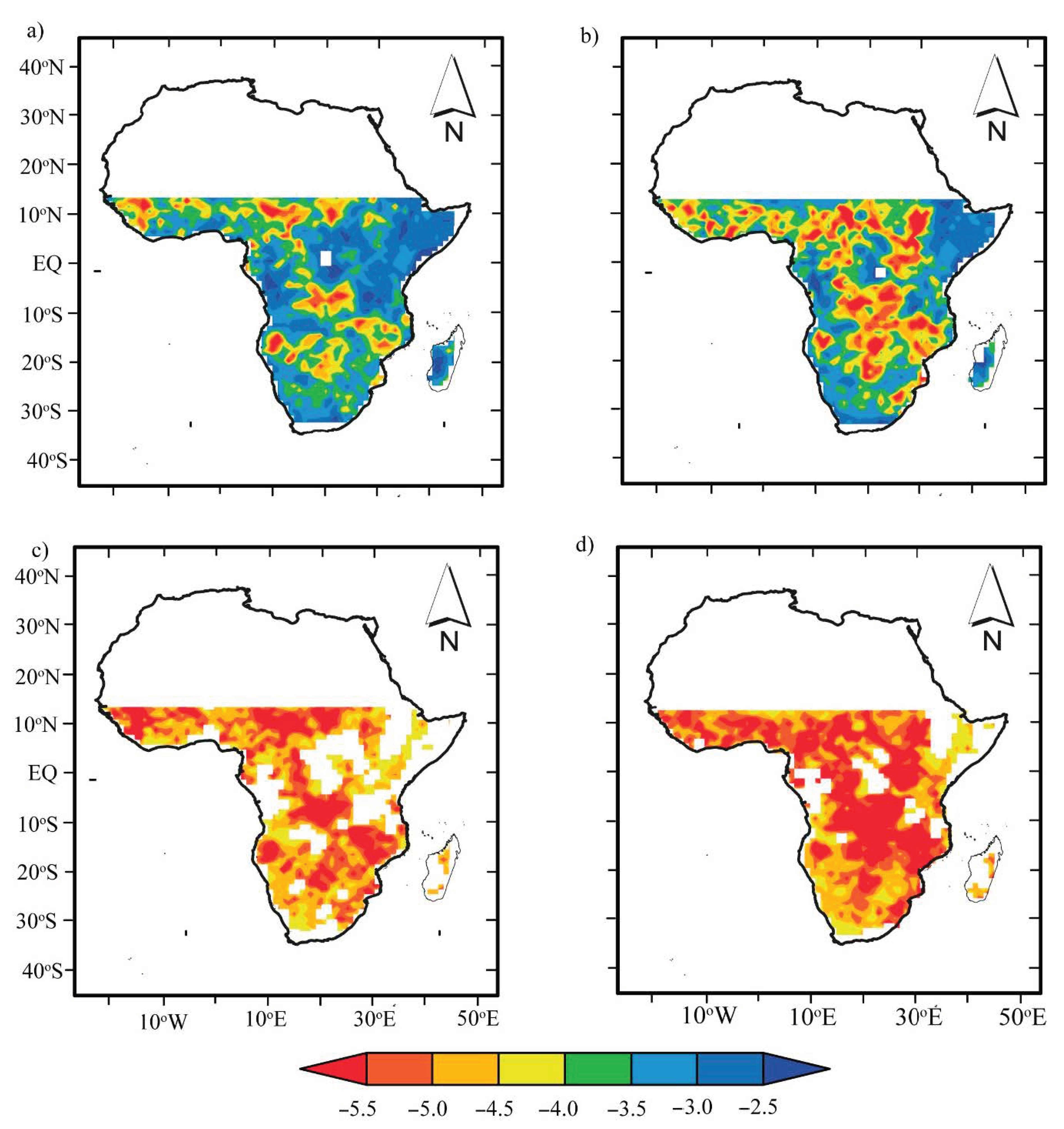
3.2. Spatial–Temporal Trends of Wetting and Drying

3.2.1. Spatial Variations in Wetting and Drying Trends

A comparison between the characteristics of the two drought datasets (scPDSIPM and scPDSITH) was made to understand how they represent trends in the wetting and drying conditions across SSA. Figure 6 shows the spatial distribution of linear trends for scPDSIPM and scPDSITH on a per-pixel basis over the period 1979–2012, estimated based on the M–K and Sen’s slope estimator. Figure 6a,b show trends of wet–dry variation from the M–K test, and Figure 6c,d show the direction of the trend based on Theil–Sen’s slope estimator.
In Figure 6a, scPDSIPM shows a spatially distinct wetting trend in SSG and parts of the SAR (in the southwest and central areas) at a rate of >0.8/10 years. The HoA shows a slightly increasing wetting trend (<0.4/10 years), mostly in the interior of the Ethiopian highlands. Similarly, in Figure 6b, scPDSITH shows slight wetting trends along the SSG and parts of the central and southwest SAR (i.e., 0.4/10 years).
Generally, we observe agreement between wetting trends in the other parts of SSA in the two datasets. The wetting trends in the SSG and SAR are mainly attributed to greening and increasing P. However, a drying trend dominates the southern part of HoA (i.e., 30°E–52°E, 0°–20°S) and the northern part of the SAR in both scPDSI datasets. Distinct drying trends are observed (decreasing) in both scPDSI datasets (Figure 6b) for many areas south of the HoA (at >1.2/10 years). In contrast, the equatorial regions and small parts of the Congo Basin and Guinea coast show drying (wetting) trends. The remaining areas present no trends in scPDSI. Both datasets show some discrepancies in wetting (drying) trends in a few areas, and we attribute these to the choice of PET measuring method used.

3.2.2. Temporal Variations in Wetting and Drying Trends

We also examined the temporal variations of regional wetting and drying conditions. We produced linear trends using the Theil–Sen slope method, and the results are presented in Figure 7. Interestingly, the interannual variations in wet and dry trends show discrepancies between the two datasets after the mid-1990s, consistent with Figure 5c,d, where similar results were observed.
In addition, we observed a widening gap between scPDSITH and scPDSIPM after the mid-1990s in the SSG and HoA, even in cases where both data sets show an increasing trend, except for the SAR, where the gap narrowed. The decline in the number of weather stations, time span, and quality of historical climate data over the SSG and HoA, as reported in [32], may explain this gap, as drought characteristics are sensitive to data time span and resolution [56], contrary to the more reliable SAR climate data (Figure 7d).

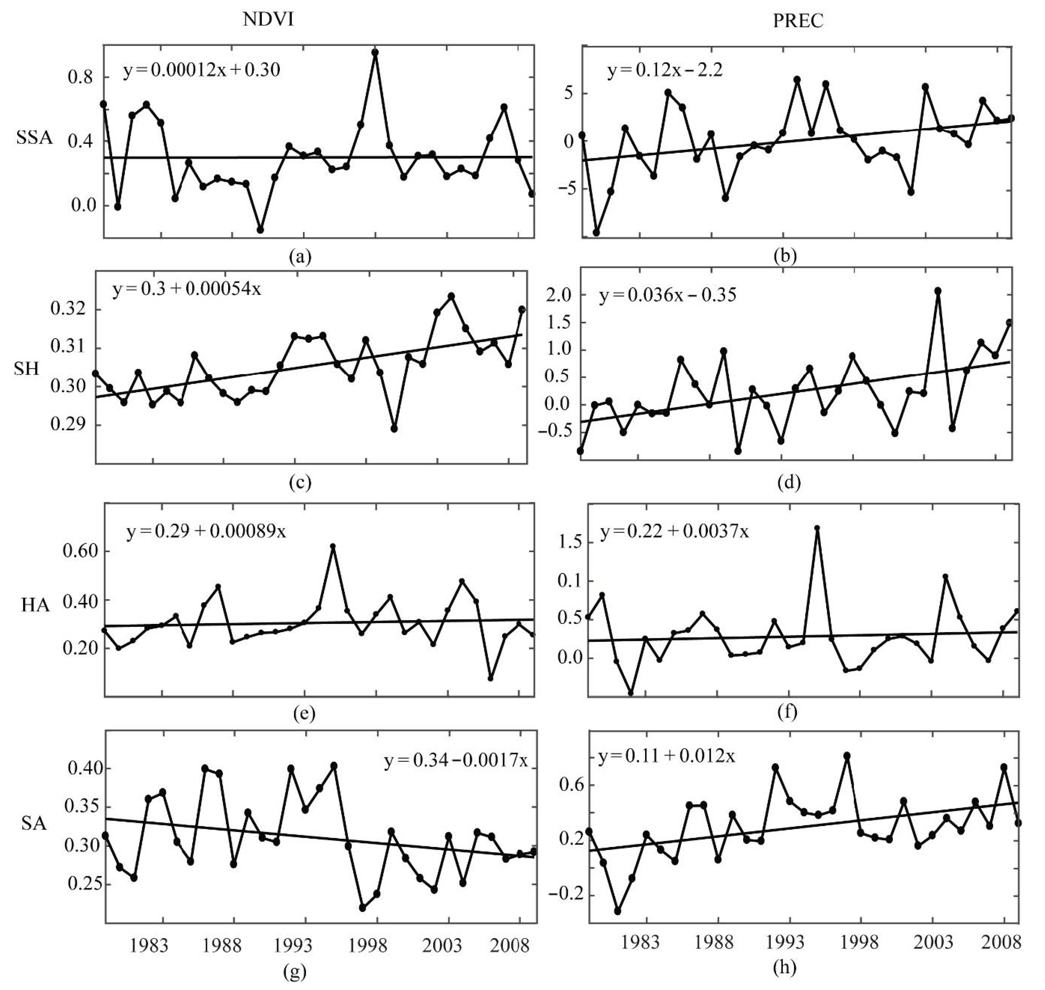
3.2.3. Temporal Variability of Remotely Sensed Precipitation and Vegetation Changes

The variability of P and NDVI were assessed to track dry spells and vegetation stress and to understand the characteristics of scPSCI variations in response to P and NDVI. Figure 8 shows the interannual variation in P and NDVI anomalies in SSA and three regions during 1982–2012 based on the regional averages of P and NDVI anomalies at each grid. Figure 8 shows that SSA P increased at a rate of 0.12 mm yr−1, whereas the SSG (at 0.036 mm yr−1) and SAR (0.012 mm yr−1) showed slight increases in P. We observed that periods with increases in P showed increasing NDVI values, which means that vegetation is usually restored to a normal status after a drought ends (except in the Figure 8e,f for HoA). This finding is consistent with wetting conditions observed in previous studies [57,58,59,60,61,62]. In these previous studies, it was concluded that, in drought conditions in arid and semi-arid regions, water availability is one of the main drivers of variations in vegetation greenness. However, the NDVI trend in the SAR showed a declining trend, while P increased over the period from 1982 to 2012. A similar result indicating a decrease in NDVI during a wet spell has been reported in [63] over the SAR and is consistent with [64], which showed that NDVI in tropical regions of Southeast Asia decreased under similar conditions.

3.3. Correlation Analysis of Dry–Wet Spells and Influencing Factors

3.3.1. Influences of Land Surface and Vegetation Variables

Changes in climate and LULC concerns are observed as challenges for land and water resource management. In this study, we characterized the relationship of hydroclimate and vegetation variables in dry and wet conditions in SSA, with a focus on P and NDVI to understand their controlling roles. We analyzed the relationships between drought and both P and NDVI. Figure 9 presents scPDSI spatial correlation results in relation to P and NDVI anomalies in SSA for the period 1982–2012 on an annual scale. The correlation results show the spatial patterns of pixels, where shaded areas denote areas where the statistical tests were significant at the 5% level (Figure 9).
In MJJASO (see Figure A1a,b), the northern part of SAA (wet) and southern part of SSA (dry) contrast shows a distinct north–south pattern with P and NDVI, and the wet/dry contrast appears to shift seasonally. Similarly, in NDJFMA (Figure A1c,d), correlation patterns changed as expected with the same significance and order of magnitude as above. This result is consistent with past studies asserting that P favors vegetation growth and that drought events may disturb vegetation growth [32]. The scPDSI spatial correlation with P was expected, as P was used in the computation of scPDSI, and the contribution of P is accounted for in the model. However, using a different P to analyze droughts’ relationships serves as a further verification step for the drought. Through this analysis, we quantify the sensitivity of drought to P changes for each grid point.

3.3.2. Influences of Teleconnections

The circulation systems are known to impact not only oceanic variability but also the climate of areas surrounding the oceans. To quantify the relationship between drought in SSA and the preceding teleconnection indices (i.e., ENSO and IOD), we performed pixel-wise correlation, and the estimated correlation was tested at a 95% significance level. Figure 10 shows pixel-wise correlation coefficients based on annual values between spatially averaged scPDSI and circulation indices (i.e., ENSO and IOD) using simple correlational analysis to understand the temporal dynamics. Overall, on an annual scale (Figure 10), both ENSO and IOD show two phases (dipole). Figure 10a,b show positive anomalies in the SSG west tips at latitudes 0°–18°S, the southern tip, and the southeast of SAR, and show negative anomalies east of 5°N–15°S. In contrast, the IOD in Figure 10c,d shows a similar order of magnitude in the phase opposite to that of ENSO, with widespread weak correlation values with respect to ENSO and IOD responses.

4. Discussion

SSA is essentially an agrarian society, where agriculture systems depend wholly on P. Thus, any delay in P in space and time places substantial demand on water availability for agricultural production and other sectors of society. There is enough evidence that the severe drought events in SSA over the years have affected millions of people, their livelihoods, and the economy [2]. However, our understanding of SSA drought characteristics, their trends, and their underlying mechanisms is largely hampered by a lack of reliable, long-term climate data from weather stations.
The recent availability of specialized global drought datasets and remote sensing makes it possible to assess drought in any location around the globe. Here, we have combined multiple dataset sources to assess drought characteristics, their trends, and their underlying mechanisms to understand drought evolution in SSA. Based on scPDSI data (based on the Penman–Monteith and Thornthwaite methods), we assessed the drought characteristics and long-term trends using Mann–Kendall and Theil–Sen slope tests in SSA over the period 1979–2012. In addition, to analyze the temporal patterns and trends of land surface variables, we used remotely sensed P and NDVI anomalies based on the M–-K and Theil–Sen slope tests. Moreover, drought events linked to land surface variables, vegetation changes, and climate circulations (i.e., ENSO and IOD) were investigated using simple correlational analysis to understand the factors that drive these drought changes in the region.
In our first analysis, we assessed drought characteristics in terms of the frequency, intensity, and affected area based on annual mean scPDSIPM and scPDSITH across SSA over the period 1979–2012. Two fixed thresholds (i.e., scPDSI < −2 and −4) were used to denote moderate and extreme droughts, respectively. These thresholds have been widely adopted and used in many studies [6,8,9,12].
Our results show that the two scPDSI datasets differed in their representation of drought characteristics across SSA. The spatial analysis (Figure 3 and Figure 4) highlight the similarity in capturing the frequency (intensity) of moderate and extreme droughts in the northwest tips of the SSG, patches north and south of the Congo basin, and patches 18°S–22°S of the Kalahari Desert to the southeast tip of Mozambique. In contrast, disagreements in the datasets were observed in a few areas in SSA that are characterized by a complex topography, large water bodies/wetlands, and dense vegetation in both scPDSI datasets.
Moderate droughts occurred more frequently than extreme droughts (see Figure 3). However, scPDSITH occurred more frequently and affected larger areas relative to scPDSIPM (Figure 3a–d). This finding is consistent with previous studies where scPDSITH exaggerated drought intensification (as it responds only to changes in T) relative to scPDSIPM (which is constrained by the inclusion of many climate variables). Similar reasons are assigned in Figure 4, but for intensity.
We further investigated the trends in drought intensities for each grid. Here, we focused on the regional trend in drought intensities over the whole SSA and three selected regions (see Figure 5a,b). Results showed an increased trend in SSA, the SSG, and the SAR, but not for the HoA, which showed stationarity in drought intensity over the period 1979–2012.
The relationship between drought frequency and areal coverage was investigated. Figure 6a,b show the interannual variation in frequency (shown as a line graph) and affected areas (shown as bar graphs) under moderate and extreme droughts. The frequency and area affected by droughts varied considerably (Figure 5a,b). This result was also reflected in Figure 6c in the temporal changes in drought intensity, but an opposite trend was found. This relation is expected, as drought intensity is related to frequency of occurrence. However, considerable disagreement was found after 1995, where both dataset estimates affected areas differently. scPDSIPM followed an opposite trend relative to scPDSITH, which is consistent with previous regional studies where the Thornthwaite method exaggerated drought frequency and intensity and hence drought-affected areas [8,55].
We analyzed the trend of wet–dry variation over the period 1979–2012 for both datasets. The findings showed varying magnitudes and trend values for the region. The spatially distinct wetting trend in Figure 7a,b is consistent with the greening and increasing P in parts of the SSA, consistent with previous studies [9]. However, some discrepancies observed in both datasets in capturing the wet/dry spells may be due to the choice of PET measurement method, consistent with past studies [9,16].
Furthermore, we investigated the trends in remotely sensed climate variables and vegetation changes to understand scPSDI variability in response to P and NDVI. We determined a regional average of P and NDVI anomalies for the whole SSA at each grid point to track dry spells and vegetation stress. Here, we used satellite data for P and NDVI products for a time span of 1982–2012 to assess the interannual variation of P and NDVI anomalies in SSA and three selected regions (see Figure 8).
Generally, there appears to be a high degree of similarity in the trends of P and NDVI in estimating wet and dry spells between both scPDSI datasets, with fluctuating increases in P and NDVI anomaly time series in both datasets (Figure 7 and Figure 8). Increased P anomalies over SSA (at a rate of 0.12 mm yr−1), the SSG (at 0.036 mm yr−1), the SAR (0.012 mm yr−1), and the HoA (0.012 mm yr−1) are consistent with wetting conditions in the region shown in previous studies on P leveling [14,21].
However, an increase in P anomalies corresponded to increased interannual variability in NDVI values, which means that vegetation is usually restored to a normal status after a dry spell ends—one exception being the SAR, where, over the period from 1982 to 2012, NDVI variability showed a declining trend and P an increasing trend. The annual P cycle in this region is tied to the passage of the West African Monsoon (WAM), which accounts for nearly 80% of the region’s annual P amount [63,64], thus exposing the region (SSG and HoA) to adverse future climate vulnerability [17,18,19,63,65]. The result of NDVI decline over the SAR is consistent with results reported in [66]. In addition, our findings further corroborate [67] on the tropical regions of Southeast Asia, where the authors found that NDVI was insensitive to drought, even during wetting spells.
In order to explain the SSA characteristics of dry–wet variation, we conducted correlation analysis to understand the relationship between scPDSI and climatic, vegetation, and atmospheric processes. The correlation results show a spatial pattern of pixels over the period 1982–2012 (annual scale in Figure 9 and seasonal scale in Figure A1 and Figure A2). Generally, a positive correlation between P (NDVI) anomalies and PDSI is widespread across the HoA, the SAR, and patches of the SSG, especially along the Guinea Coast at annual and seasonal scales. A seasonal shift from northern and southern part of SSA was observed for monsoon P anomalies in response to PDSI (Figure A1). We found that MJJASO (Figure A1a,b) sensitivities were evident largely in the SSG, while those of NDJFMA (Figure A1c,d) were evident in the SAR and HoA. Similarly, in Figure A2, the NDVI anomalies in relation to PDSI are consistent with P anomalies, but at varying magnitudes in space. This finding is consistent with both the annual and seasonal climatology of P and NDVI and underscores these two variables as major influencing variables with respect to extreme events in SSA. Our findings are consistent with analyses of the SPEI and NDVI relationship in [68], wherein it was concluded that water availability is the determinant factor for vegetation change in different climate regions of Southeast Asia.
Last but not least, previous studies have attempted to link drought episodes to climate circulations (see [56] in the case of the USA). Regarding SSA, both Sheffield [23] and Katchele [22] mentioned that studying the links between droughts and teleconnections is useful but remains a key challenge. We performed pixel-wise correlation to understand the temporal dynamics (Figure 10). The result showed that ENSO and IOD have a significant impact on wet and dry spells and that their geographical impact is consistent with that of P and NDVI anomalies. Despite weak correlation values, this result agrees with similar studies linking drought episodes to ENSO and IOD in Africa [31,32]. A negative (positive) correlation is associated with strong La Niña (El Niño) events, enhancing (reducing) P and hence wet (dry) spells. Similarly, IOD, as a coupled ocean–atmosphere mode, indicates a negative (positive) phase described by cool (warm) SSTs and impacts drought episodes in places consistent with ENSO but in an opposite phase (Figure 10c,d, bottom panel).

5. Conclusions

We assessed the impact of different PET methods (i.e., scPDSIPM and scPDSITH) on long-term drought trends and used remotely sensed P, vegetation change, and observed climate circulation indices (i.e., ENSO and IOD) to investigate how these variables respond to droughts across SSA. Compared to previous regional drought assessments of SSA, we summarize noteworthy novelties:
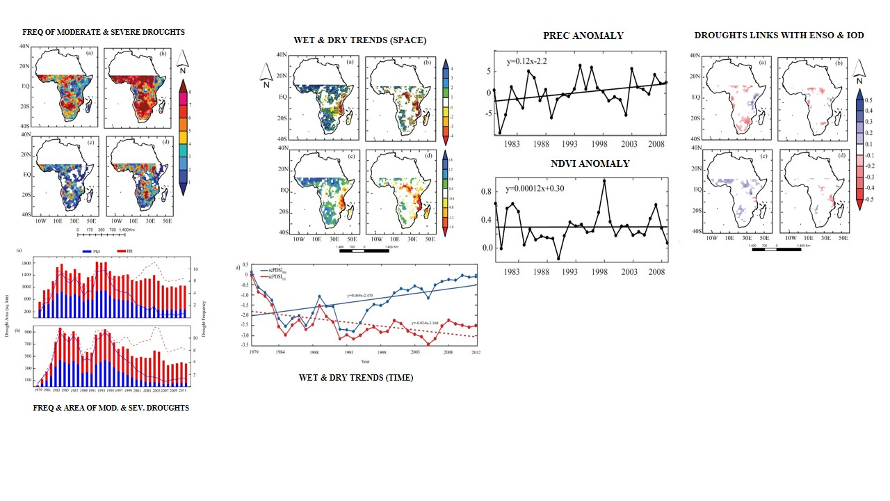
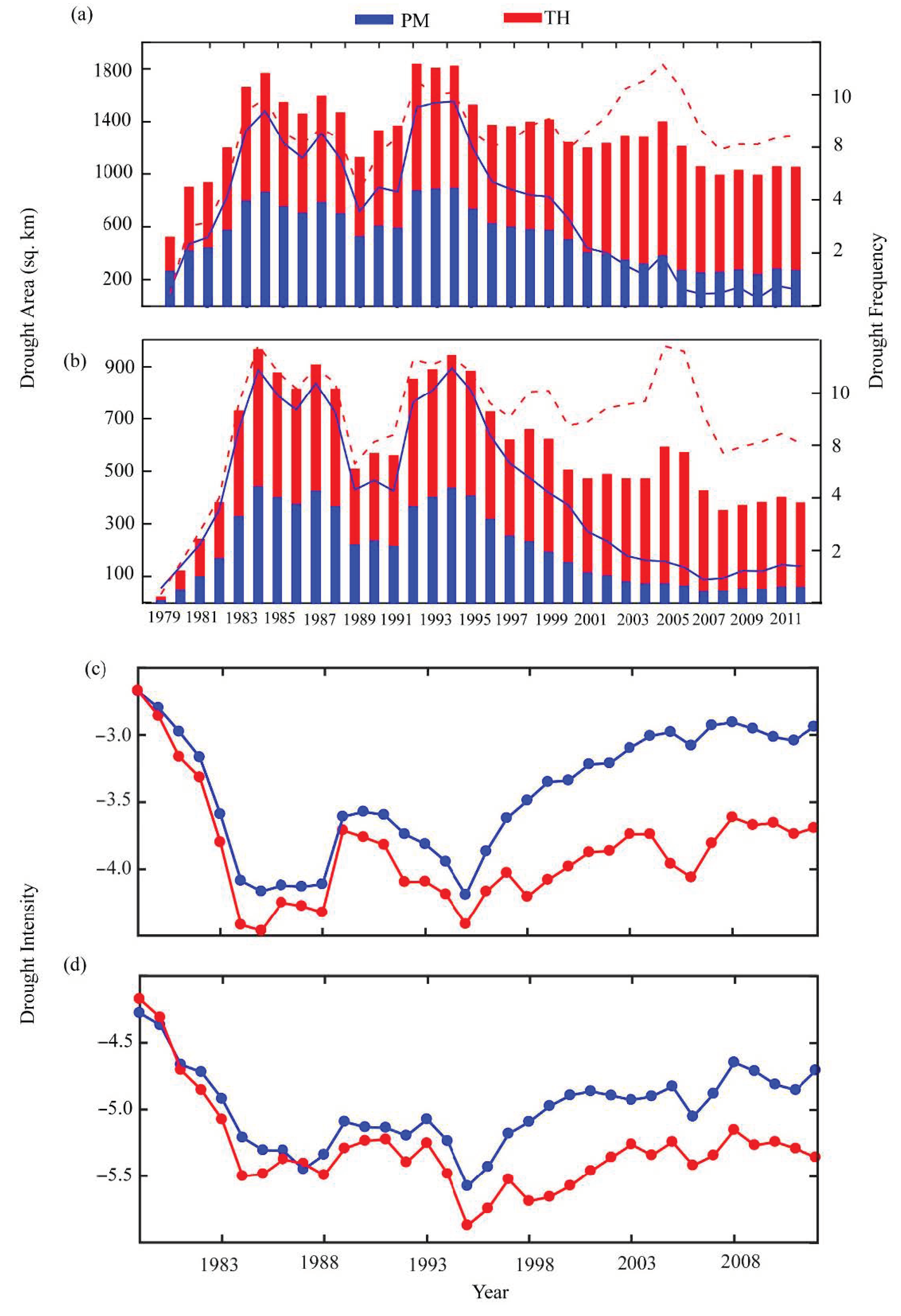
  • The spatial analysis of scPDSITH and scPDSIPM differed in their representation of drought characteristics (i.e., frequency, affected area, and intensity) across SSA. The interannual variations in moderate droughts showed a decreasing trend and, after the mid-1990s, an abrupt change toward an increasing trend. We found similar results in the extreme drought data.
  • Both scPDSI data sets showed significant drying trends in drought intensity and an increasing trend in the affected areas. However, the Thornthwaite method exaggerated droughts relative to the Penman–Monteith method in the warming climate.
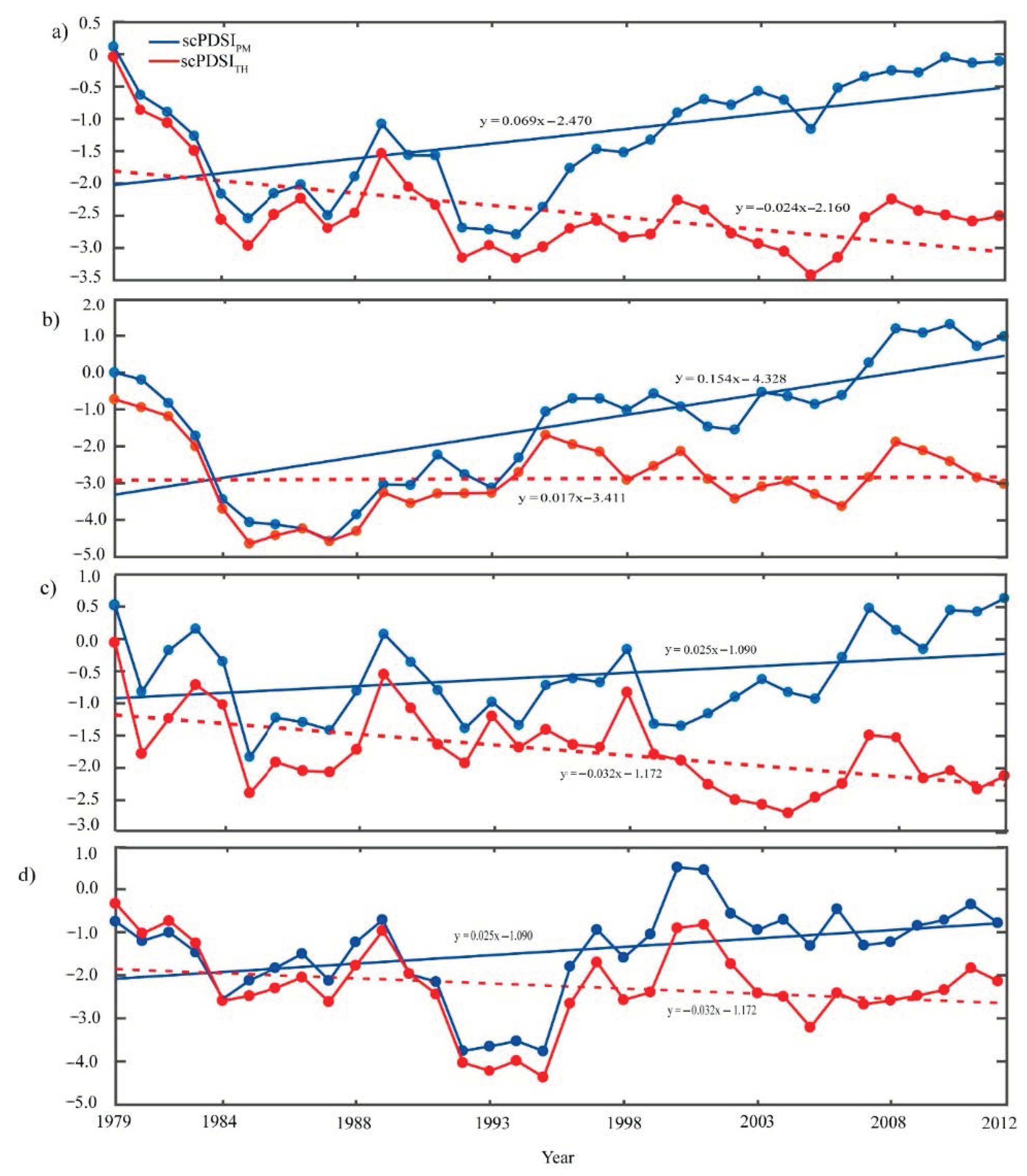
  • Generally, increased wet spells found in transition and dry climatic regions across SSA are due to increased P. The wet and dry trends were consistent and significant in both datasets over SSA, where a downward trend (1979–1995) indicates increased intensity, and an upward trend (1995–2012) suggests decreased intensity. These findings suggest that floods and droughts have become more frequent in recent times as a result of global warming.
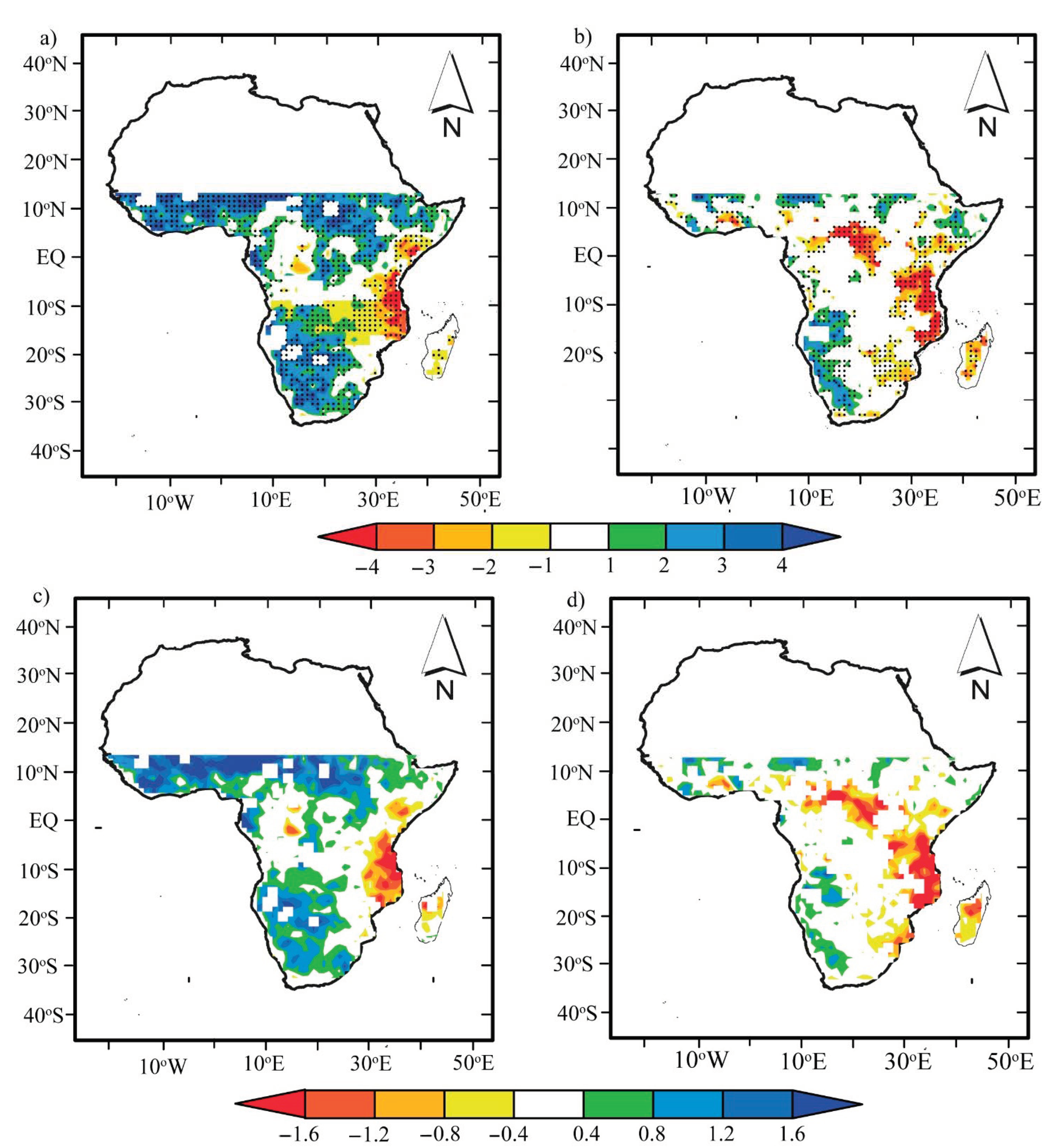
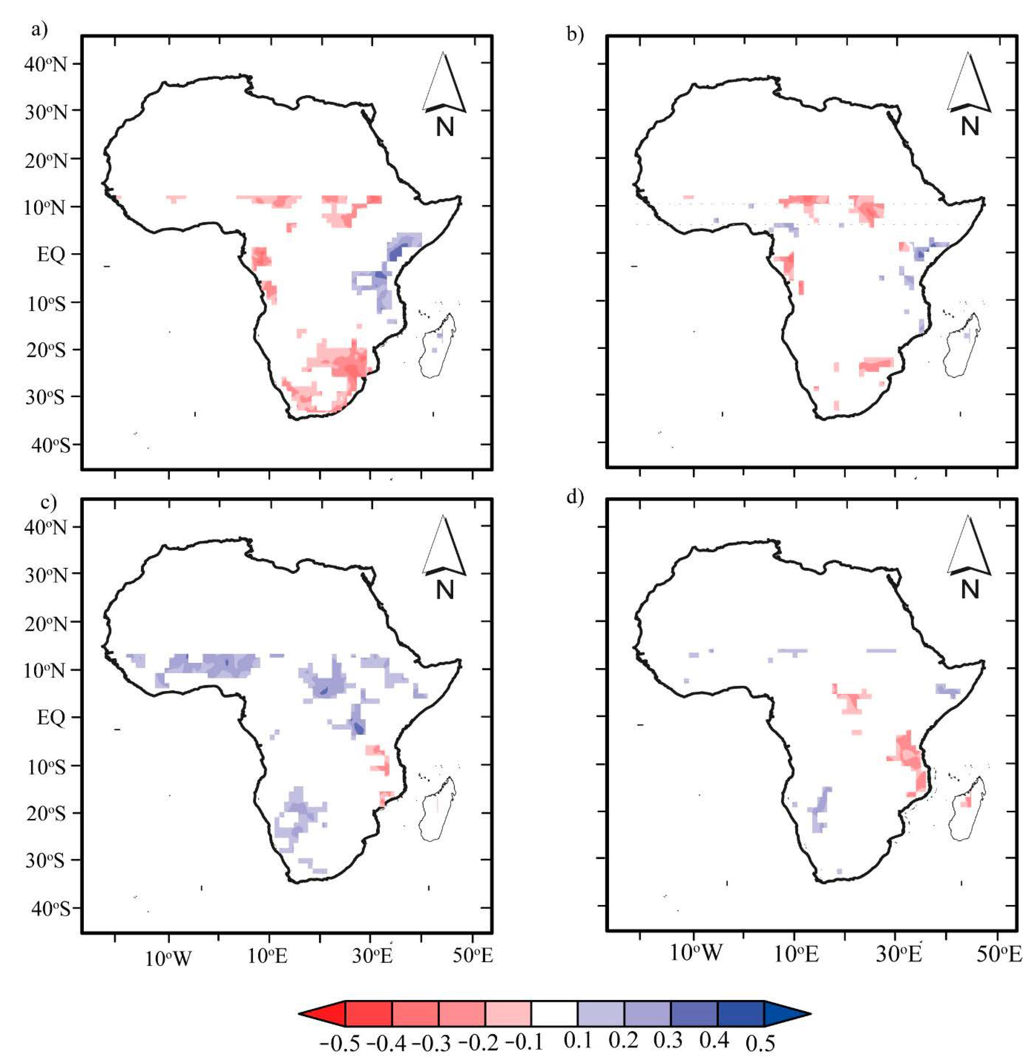
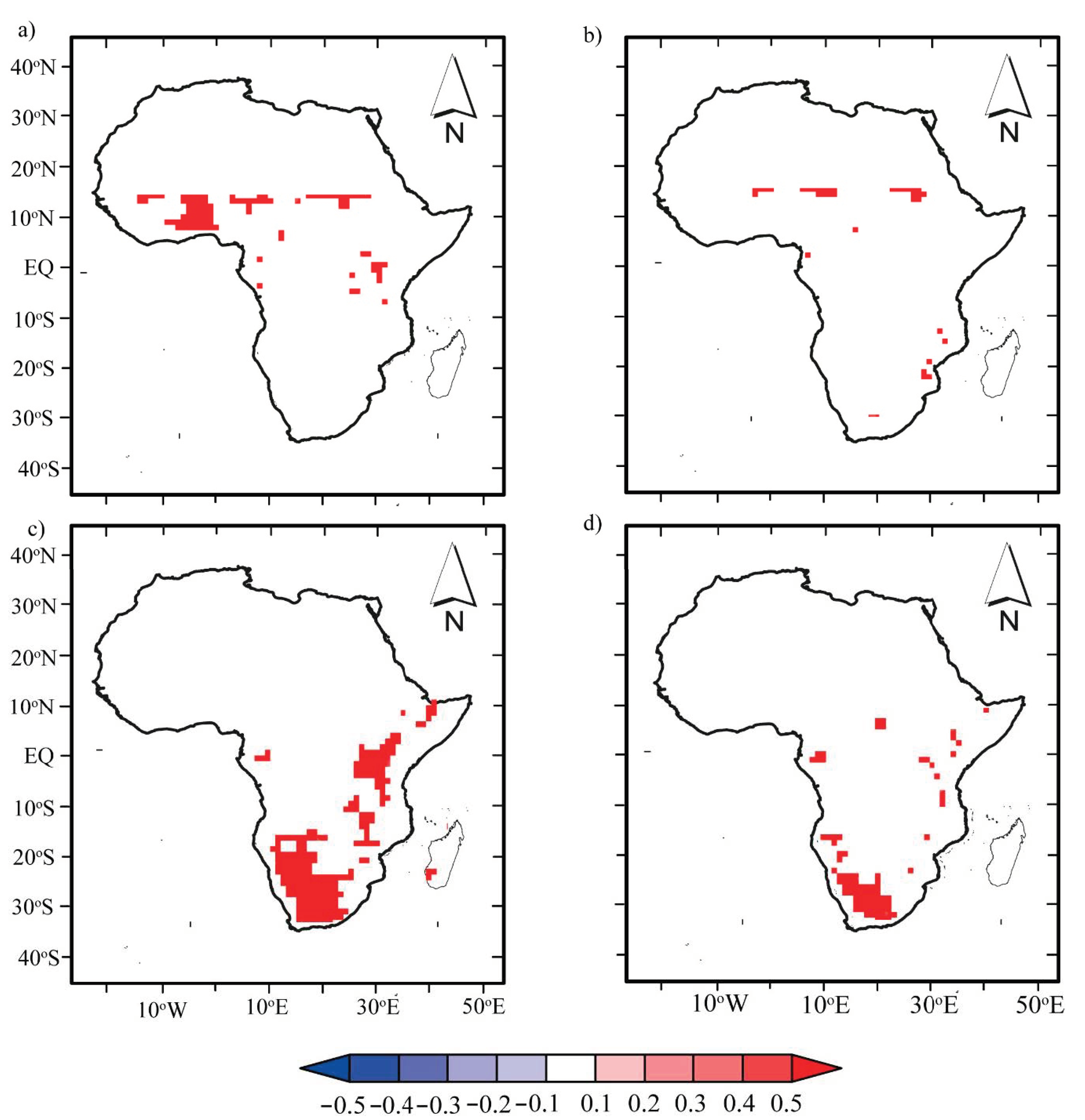
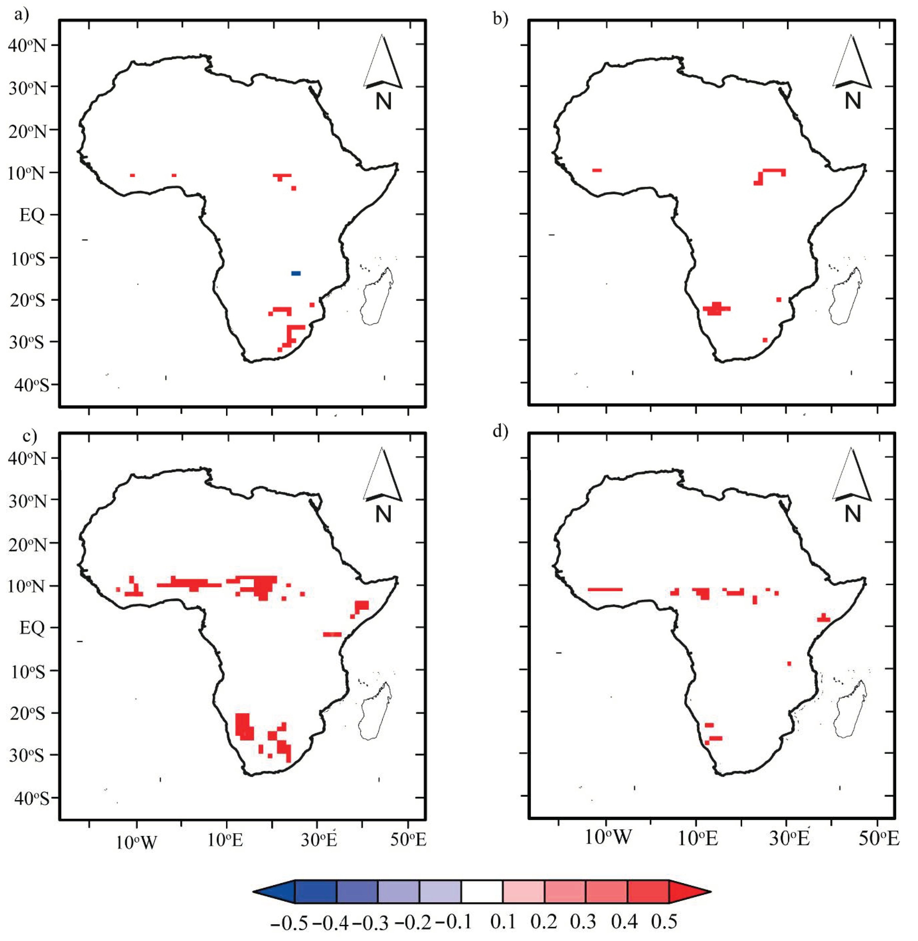
  • A general negative correlation between P anomalies and PDSI was found across SSA, with the strongest relationships in locations along the SSG, HoA, and SAR. Positive correlations of NDVI anomalies and PDSI across SSA tend to be in small patches with modest exceptions during monsoon and post-monsoon seasons in the SSG, HoA, and SAR. In addition, PDSI is impacted by ENSO and IOD, with a similar overlap in geographic distributions.

Author Contributions

Conceptualization: I.K.N. and G.W.; data curation: I.K.N., G.W., and J.L.; methodology: I.K.N., G.W., D.F.T.H., and J.L.; resources: G.W.; supervision: G.W. and D.F.T.H.; validation: D.F.T.H., W.U., and S.L.; visualization: A.S.B., X.S., D.L., and C.Z.; writing—original draft: I.K.N.; writing—review and editing: G.W., D.F.T.H., N.A.P., K.T.C.L.K.S., M.D., and S.O.Y.A. All authors have read and agreed to the published version of the manuscript.

Funding

There is no funding for this research.

Data Availability Statement

The data presented in this study are available on request from the corresponding author.

Acknowledgments

We extend our gratitude to the developers, managers, and funding agencies of the Terrestrial Hydrology Research Group (Princeton University), the Climate Hazards Group (CHIRPS), ECMWF (ERA-5), the GIMMS group (NDVI data), the ESACCI group (LULC map), the NASA-SRTM group (DEM), and the Climate Prediction Center (ENSO and IOD data) for granting access to these datasets in accordance with their specific data use and citation policies.

Conflicts of Interest

The authors declare no conflict of interest.

Appendix A

Figure A1. Pixel-wise correlation coefficients between seasonal mean scPDSI with the seasonal mean P anomalies in SSA for period 1982–2012: (a) MJJASO scPDSIPM and P anomaly, (b) MJJASO PDSITH and P anomaly, (c) NDJFMA scPDSIPM and P anomaly, and (d) NDJFMA scPDSITH and P anomaly. The shaded areas denote areas where the statistical tests were significant at the 5% level, and areas that are not significant at the 5% level are masked out (white shading).
Remotesensing 13 00533 g0a1
Figure A2. Pixel-wise correlation coefficients between seasonal mean scPDSI with the seasonal mean NDVI anomalies in SSA for period 1982–2012: (a) MJJASO scPDSIPM and NDVI anomaly, (b) MJJASO PDSITH and NDVI anomaly (c) NDJFMA scPDSIPM and NDVI anomaly, and (d) NDJFMA scPDSITH and NDVI anomaly. The shaded areas denote areas where the statistical tests were significant at the 5% level, and areas that are not significant at the 5% level are masked out (white shadings).
Remotesensing 13 00533 g0a2

References

  1. IPCC. Climate Change 2014: Impacts, Adaptation, and Vulnerability; Barros, R.V., Field, C.B., Dokken, D.J., Mastrandrea, M.D., Mach, K.J., Bilir, T.E., Ebi, K.L., Estrada, Y.O., Genova, R.C., Girma, B., et al., Eds.; Cambridge University Press: Cambridge, UK; New York, NY, USA, 2014. [Google Scholar]
  2. Guha-Sapir, D.; Below, R.; Hoyois, P. Emem-Dat: The International Disaster Database. Available online: https://www.emdat.be/ (accessed on 6 January 2020).
  3. Bachmair, S.; Svensson, C.; Hannaford, J.; Barker, L.J.; Stahl, K. A quantitative analysis to objectively appraise drought indicators and model drought impacts. Hydrol. Earth Syst. Sci. 2016, 20, 2589–2609. [Google Scholar] [CrossRef] [Green Version]
  4. Bachmair, S.; Tanguy, M.; Hannaford, J.; Stahl, K. How well do meteorological indicators represent agricultural and forest drought across europe? Environ. Res. Lett. 2018, 13, 034042. [Google Scholar] [CrossRef]
  5. Paulo, A.A.; Rosa, R.D.; Pereira, L.S. Climate trends and behaviour of drought indices based on precipitation and evapotranspiration in portugal. Nat. Hazards Earth Syst. Sci. 2012, 12, 1481–1491. [Google Scholar] [CrossRef]
  6. Vicente-Serrano, S.M.; Beguería, S.; Lorenzo-Lacruz, J.; Camarero, J.J.; López-Moreno, J.I.; Azorin-Molina, C.; Revuelto, J.; Morán-Tejeda, E.; Sanchez-Lorenzo, A. Performance of drought indices for ecological, agricultural, and hydrological applications. Earth Interact. 2012, 16, 1–27. [Google Scholar] [CrossRef] [Green Version]
  7. Mishra, A.K.; Singh, V.P. A review of drought concepts. J. Hydrol. 2010, 391, 202–216. [Google Scholar] [CrossRef]
  8. Dai, A. Increasing drought under global warming in observations and models. Nat. Clim. Change 2013, 3, 52–58. [Google Scholar] [CrossRef]
  9. Sheffield, J.; Wood, E.F.; Roderick, M.L. Little change in global drought over the past 60 years. Nature 2012, 491, 435–438. [Google Scholar] [CrossRef]
  10. Seneviratne, S.I. Historical drought trends revisited. Nature 2012, 491, 338–339. [Google Scholar] [CrossRef]
  11. Trenberth, K.E.; Dai, A.; van der Schrier, G.; Jones, P.D.; Barichivich, J.; Briffa, K.R.; Sheffield, J. Global warming and changes in drought. Nat. Clim. Change 2014, 4, 17–22. [Google Scholar] [CrossRef]
  12. Dai, A.; Trenberth, K.E.; Qian, T. A global dataset of palmer drought severity index for 1870–2002: Relationship with soil moisture and effects of surface warming. J. Hydrometeorol. 2004, 5, 1117–1130. [Google Scholar] [CrossRef]
  13. Chen, T.; van der Werf, G.R.; de Jeu, R.A.M.; Wang, G.; Dolman, A.J. A global analysis of the impact of drought on net primary productivity. Hydrol. Earth Syst. Sci. 2013, 17, 3885–3894. [Google Scholar] [CrossRef] [Green Version]
  14. Chen, T.; Zhang, H.; Chen, X.; Hagan, D.F.; Wang, G.; Gao, Z.; Shi, T. Robust drying and wetting trends found in regions over china based on köppen climate classifications. J. Geophys. Res. Atmos. 2017, 122, 4228–4237. [Google Scholar] [CrossRef]
  15. Heim, R.R., Jr. A review of twentieth-century drought indices used in the united states. Bull. Am. Meteorol. Soc. 2002, 83, 1149–1166. [Google Scholar] [CrossRef] [Green Version]
  16. Wang, G.; Gong, T.; Lu, J.; Lou, D.; Hagan, D.F.T.; Chen, T. On the long-term changes of drought over china (1948–2012) from different methods of potential evapotranspiration estimations. Int. J. Climatol. 2018, 38, 2954–2966. [Google Scholar] [CrossRef]
  17. Ajayi, V.O.; Ilori, O.W. Projected Drought Events over West Africa Using RCA4 Regional Climate Model. Earth Syst. Environ. 2020, 4, 329–348. [Google Scholar] [CrossRef]
  18. Quenum, G.M.L.D.; Klutse, N.A.B.; Dieng, D.; Laux, P.; Arnault, J.; Kodja, J.D.; Oguntunde, P.G. Identification of Potential Drought Areas in West Africa Under Climate Change and Variability. Earth Syst. Environ. 2019, 3, 429–444. [Google Scholar] [CrossRef] [Green Version]
  19. Driouech, F.; ElRhaz, K.; Moufouma-Okia, W.; Arjdal, K.; Balhane, S. Assessing Future Changes of Climate Extreme Events in the CORDEX-MENA Region Using Regional Climate Model ALADIN-Climate. Earth Syst. Environ. 2020, 4, 477–492. [Google Scholar] [CrossRef]
  20. Sun, Q.; Miao, C.; Duan, Q.; Ashouri, H.; Sorooshian, S.; Hsu, K.-L. A review of global precipitation data sets: Data sources, estimation, and intercomparisons. Rev. Geophys. 2018, 56, 79–107. [Google Scholar] [CrossRef] [Green Version]
  21. Sun, B.; Gao, Z.; Li, Z.; Wang, H.; Li, X.; Wang, B.; Wu, J. Dynamic and dry/wet variation of climate in the potential extent of desertification in china during 1981–2010. Environ. Earth Sci. 2015, 73, 3717–3729. [Google Scholar] [CrossRef]
  22. Faustin Katchele, O.; Ma, Z.-G.; Yang, Q.; Batebana, K. Comparison of trends and frequencies of drought in central north china and sub-saharan africa from 1901 to 2010. Atmos. Ocean. Sci. Lett. 2017, 10, 418–426. [Google Scholar] [CrossRef] [Green Version]
  23. Sheffield, J.; Wood, E.F.; Chaney, N.; Guan, K.; Sadri, S.; Yuan, X.; Olang, L.; Amani, A.; Ali, A.; Demuth, S.; et al. A drought monitoring and forecasting system for sub-sahara african water resources and food security. Bull. Am. Meteorol. Soc. 2014, 95, 861–882. [Google Scholar] [CrossRef]
  24. FAO. The State of Food and Agriculture 2016; Food and Agriculture of the United Nations: Rome, Italy, 2016; p. 196. [Google Scholar]
  25. Van Loon, A.F. Hydrological drought explained. WIREs Water 2015, 2, 359–392. [Google Scholar] [CrossRef]
  26. Schellekens, J.; Dutra, E.; Martínez-de la Torre, A.; Balsamo, G.; van Dijk, A.; Sperna Weiland, F.; Minvielle, M.; Calvet, J.C.; Decharme, B.; Eisner, S.; et al. A global water resources ensemble of hydrological models: The earth2observe tier-1 dataset. Earth Syst. Sci. Data 2017, 9, 389–413. [Google Scholar] [CrossRef] [Green Version]
  27. Beck, H.E.; Zimmermann, N.E.; McVicar, T.R.; Vergopolan, N.; Berg, A.; Wood, E.F. Present and future köppen-geiger climate classification maps at 1-km resolution. Sci. Data 2018, 5, 180214. [Google Scholar] [CrossRef] [PubMed] [Green Version]
  28. ESACCI. European Space Agency Climate Change Initiative. Land Use Land Cover (Lulc) Map. Available online: https://www.esa-landcover-cci.org/ (accessed on 10 November 2019).
  29. Camberlin, P.; Philippon, N. The east african march–may rainy season: Associated atmospheric dynamics and predictability over the 1968–97 period. J. Clim. 2002, 15, 1002–1019. [Google Scholar] [CrossRef]
  30. Ullah, W.; Wang, G.; Lou, D.; Ullah, S.; Bhatti, A.S.; Ullah, S.; Karim, A.; Hagan, D.F.T.; Ali, G. Large-scale atmospheric circulation patterns associated with extreme monsoon precipitation in Pakistan during 1981–2018. Atmos. Res. 2021, 105489. [Google Scholar] [CrossRef]
  31. Poccard, I.; Janicot, S.; Camberlin, P. Comparison of rainfall structures between ncep/ncar reanalyses and observed data over tropical africa. Clim. Dyn. 2000, 16, 897–915. [Google Scholar] [CrossRef]
  32. Philippon, N.; Martiny, N.; Camberlin, P.; Hoffman, M.T.; Gond, V. Timing and patterns of the enso signal in africa over the last 30 years: Insights from normalized difference vegetation index data. J. Clim. 2014, 27, 2509–2532. [Google Scholar] [CrossRef]
  33. National Aeronautics and Space Administration (NASA) Shuttle Radar Topography Mission (SRTM) Home Page. Available online: https://lpdaac.usgs.gov/products/srtmgl1v003/ (accessed on 10 November 2019).
  34. Palmer, W. Meteorological Drought; US Weather Bureau: Washington, DC, USA, 1965. [Google Scholar]
  35. Terrestrial Hydrology Research Group. A Global Dataset of Palmer Drought Severity Index and Potential Evaporation at 1.0-Degree, Monthly Resolution. Available online: http://hydrology.princeton.edu/data/pdsi/updates_1948-2012/ (accessed on 10 November 2019).
  36. Sheffield, J.; Goteti, G.; Wood, E.F. Development of a 50-year high-resolution global dataset of meteorological forcings for land surface modeling. J. Clim. 2006, 19, 3088–3111. [Google Scholar] [CrossRef] [Green Version]
  37. Tucker, C.J.; Pinzon, J.E.; Brown, M.E.; Slayback, D.A.; Pak, E.W.; Mahoney, R.; Vermote, E.F.; El Saleous, N. An extended avhrr 8-km ndvi dataset compatible with modis and spot vegetation NDVI data. Int. J. Remote Sens. 2005, 26, 4485–4498. [Google Scholar] [CrossRef]
  38. Martiny, N.; Camberlin, P.; Richard, Y.; Philippon, N. Compared regimes of NDVI and rainfall in semi-arid regions of Africa. Int. J. Remote Sens. 2006, 27, 5201–5223. [Google Scholar] [CrossRef]
  39. Funk, C.; Peterson, P.; Landsfeld, M.; Pedreros, D.; Verdin, J.; Shukla, S.; Husak, G.; Rowland, J.; Harrison, L.; Hoell, A.; et al. The climate hazards infrared precipitation with stations—A new environmental record for monitoring extremes. Sci. Data 2015, 2, 150066. [Google Scholar] [CrossRef] [PubMed] [Green Version]
  40. IRI/LDE. International Research Institute Climate Data Library. Available online: https://iri.columbia.edu/topics/data-library/ (accessed on 10 November 2019).
  41. Funk, C.C.; Peterson, P.J.; Landsfeld, M.F.; Pedreros, D.H.; Verdin, J.P.; Rowland, J.D.; Romero, B.E.; Husak, G.J.; Michaelsen, J.C.; Verdin, A.P. A Quasi-Global Precipitation Time Series for Drought Monitoring; USGS: Reston, VA, USA, 2014; p. 4. [Google Scholar]
  42. Agutu, N.O.; Awange, J.L.; Zerihun, A.; Ndehedehe, C.E.; Kuhn, M.; Fukuda, Y. Assessing multi-satellite remote sensing, reanalysis, and land surface models’ products in characterizing agricultural drought in East Africa. Remote Sens. Environ. 2017, 194, 287–302. [Google Scholar] [CrossRef] [Green Version]
  43. Ullah, W.; Wang, G.; Ali, G.; Tawia Hagan, D.F.; Bhatti, A.S.; Lou, D. Comparing multiple precipitation products against in-situ observations over different climate regions of Pakistan. Remote Sens. 2019, 11, 628. [Google Scholar] [CrossRef] [Green Version]
  44. Climate Prediction Center (CPC) of the National Weather Service. U.S.w. Available online: http://www.Cpc.Ncep.Noaa.Gov (accessed on 6 January 2020).
  45. Climate Prediction Center (CPC) of the National Weather Service. Database. Available online: http://www.cpc.ncep.noaa.gov/data/indices/ (accessed on 6 January 2020).
  46. Smith, T.M.; Reynolds, R.W.; Peterson, T.C.; Lawrimore, J. Improvements to noaa’s historical merged land–ocean surface temperature analysis (1880–2006). J. Clim. 2008, 21, 2283–2296. [Google Scholar] [CrossRef]
  47. European Center for Medium-Range Weather Forecasts (ECMWF) Home Page. Available online: http://apps.ecmwf.int/datasets/data/interim-full-daily/levtype=sfc/ (accessed on 10 November 2019).
  48. Shlien, S. Geometric correction, registration, and resampling of landsat imagery. Can. J. Remote Sens. 1979, 5, 74–89. [Google Scholar] [CrossRef]
  49. Nooni, I.K.; Duker, A.A.; Van Duren, I.; Addae-Wireko, L.; Osei Jnr, E.M. Support vector machine to map oil palm in a heterogeneous environment. Int. J. Remote Sens. 2014, 35, 4778–4794. [Google Scholar] [CrossRef]
  50. Mann, H.B. Nonparametric tests against trend. Econometrica 1945, 13, 245–259. [Google Scholar] [CrossRef]
  51. Kendall, M.G. Rank Correlation Methods; Charles Griffin: London, UK, 1975. [Google Scholar]
  52. Sen, P.K. Estimates of the regression coefficient based on kendall’s tau. J. Am. Stat. Assoc. 1968, 63, 1379–1389. [Google Scholar] [CrossRef]
  53. Nooni, I.K.; Wang, G.; Hagan, D.F.T.; Lu, J.; Ullah, W.; Li, S. Evapotranspiration and its components in the nile river basin based on long-term satellite assimilation product. Water 2019, 11, 1400. [Google Scholar] [CrossRef] [Green Version]
  54. Klein Tank, A.M.G.; Zwiers, F.W.; Zhang, X. Guidelines on Analysis of Extremes in a Changing Climate in Support of Informed Decisions for Adaptation; WMO-TD No. 1500; World Meteorological Organization: Geneva, Switzerland, 2012. [Google Scholar]
  55. Zhai, J.; Su, B.; Krysanova, V.; Vetter, T.; Gao, C.; Jiang, T. Spatial variation and trends in PDSI and SPI indices and their relation to streamflow in 10 large regions of china. J. Clim. 2010, 23, 649–663. [Google Scholar] [CrossRef]
  56. Golian, S.; Javadian, M.; Behrangi, A. On the use of satellite, gauge, and reanalysis precipitation products for drought studies. Environ. Res. Lett. 2019, 14, 075005. [Google Scholar] [CrossRef]
  57. Klein, T. Drought-induced tree mortality: From discrete observations to comprehensive research. Tree Physiol. 2015, 35, 225–228. [Google Scholar] [CrossRef] [PubMed] [Green Version]
  58. McDowell, N.G. Mechanisms linking drought, hydraulics, carbon metabolism, and vegetation mortality. Plant Physiol. 2011, 155, 1051–1059. [Google Scholar] [CrossRef] [Green Version]
  59. McDowell, N.; Pockman, W.T.; Allen, C.D.; Breshears, D.D.; Cobb, N.; Kolb, T.; Plaut, J.; Sperry, J.; West, A.; Williams, D.G.; et al. Mechanisms of plant survival and mortality during drought: Why do some plants survive while others succumb to drought? New Phytol. 2008, 178, 719–739. [Google Scholar] [CrossRef]
  60. Xu, C.; McDowell, N.G.; Fisher, R.A.; Wei, L.; Sevanto, S.; Christoffersen, B.O.; Weng, E.; Middleton, R.S. Increasing impacts of extreme droughts on vegetation productivity under climate change. Nat. Clim. Change 2019, 9, 948–953. [Google Scholar] [CrossRef] [Green Version]
  61. Ivits, E.; Horion, S.; Fensholt, R.; Cherlet, M. Drought footprint on European ecosystems between 1999 and 2010 assessed by remotely sensed vegetation phenology and productivity. Glob. Change Biol. 2014, 20, 581–593. [Google Scholar] [CrossRef]
  62. Zhang, B.; Zhang, L.; Guo, H.; Leinenkugel, P.; Zhou, Y.; Li, L.; Shen, Q. Drought impact on vegetation productivity in the Lower Mekong Basin. Int. J. Remote Sens. 2014, 35, 2835–2856. [Google Scholar] [CrossRef]
  63. Dosio, A.; Turner, A.G.; Tamoffo, A.T.; Sylla, M.B.; Lennard, C.; Jones, R.G.; Terray, L.; Nikulin, G.; Hewitson, B. A tale of two futures: Contrasting scenarios of future precipitation for West Africa from an ensemble of regional climate models. Environ. Res. Lett. 2020, 15, 064007. [Google Scholar] [CrossRef]
  64. Steinig, S.; Harlaß, J.; Park, W.; Latif, M. Sahel rainfall strength and onset improvements due to more realistic Atlantic cold tongue development in a climate model. Sci. Rep. 2018, 8, 2569. [Google Scholar] [CrossRef] [Green Version]
  65. Barros, R.V.; Field, C.B.; Dokken, D.J.; Mastrandrea, M.D.; Mach, K.J.; Bilir, T.E.; Ebi, K.L.; Estrada, Y.O.; Genova, R.C.; Girma, B.; et al. (Eds.) Climate Change 2014: Impacts, Adaptation, and Vulnerability. Part B: Regional Aspects; Contribution of Working Group II to the Fifth Assessment Report of the Intergovernmental Panel on Climate Change; Cambridge University Press: Cambridge, UK, 2014; pp. 1199–1265. [Google Scholar]
  66. Anyamba, A.; Tucker, C.J.; Eastman, J.R. NDVI anomaly patterns over Africa during the 1997/98 ENSO warm event. Int. J. Remote Sens. 2001, 22, 1847–1859. [Google Scholar]
  67. Zhang, Y.; Zhu, Z.; Liu, Z.; Zeng, Z.; Ciais, P.; Huang, M.; Liu, Y.; Piao, S. Seasonal and interannual changes in vegetation activity of tropical forests in Southeast Asia. Agric. For. Meteorol. 2016, 224, 1–10. [Google Scholar] [CrossRef]
  68. Zhang, Q.; Kong, D.; Singh, V.P.; Shi, P. Response of vegetation to different time-scales drought across China: Spatiotemporal patterns, causes and implications. Glob. Planet. Change 2017, 152, 1–11. [Google Scholar] [CrossRef] [Green Version]
Figure 1. (ad) The administrative boundary of Continental Africa: (a) topography at 30 m resolution acquired from a Shuttle Radar Topography Mission (SRTM) digital elevation model (DEM) of the National Aeronautics and Space Administration (NASA) [33]; (b) 2016 land use land cover (LULC) map at a 20 m resolution acquired from the European Space Agency Climate Change Initiative (ESACCI) (see Table 1 for details) [28]; (c,d) spatial distribution of annual average Climate Hazard Group Infrared Precipitation with Stations (CHIRPS) P and ERA-5 T over the period 1981–2017. (e,f) Multi-year (1981–2017) (e) precipitation (P) and (f) temperature (T) averaged monthly.
Remotesensing 13 00533 g001
Figure 2. Drought frequency in Sub-Saharan Africa (SSA) over the period 1979–2012 for (a) scPDSIPM < −2, (b) scPDSITH < −2, (c) scPDSIPM < −4, and (d) scPDSITH < −4.
Remotesensing 13 00533 g002
Figure 3. Drought intensity in SSA over the period 1979–2012 for (a) scPDSIPM < −2, (b) scPDSITH < −2, (c), scPDSIPM < −4, and (d) PDSITH < −4.
Remotesensing 13 00533 g003
Figure 4. Interannual variation of drought intensity for drought category in SSA over the period 1979–2012 for (a) scPDSIPM < −2, (b) scPDSITH < −2, (c) scPDSIPM < −4, and (d) scPDSITH < −4. SSA (black lines), the Sudano-Sahelian–Guinean coast (SSG) (brown lines), the HoA (gold lines), and Southern Africa region (SAR) (red lines).
Remotesensing 13 00533 g004
Figure 5. Drought frequency–areal extent relationship based on regional average time series in SSA. (a) Frequency–areal extent relationship for PDSI < −2; (b) frequency–areal extent relationship for scPDSI < −4 over the period 1979–2012; (c) the drought intensity of scPDSI < −2; (d) the drought intensity of scPDSI < −4 over the period of 1979–2012. The blue lines indicate scPDSIPM and the red lines indicate scPDSITH.
Remotesensing 13 00533 g005
Figure 6. Pixel-wise linear trends using the Mann–Kendall (a,b) and Theil–Sen slope methods (c,d) over the period 1979–2012 for (a,c) scPDSIPM and (b,d) scPDSITH. Values are expressed in changes per decade. A positive value indicates wetting and a negative indicates drying. Shading indicates that correlations are significant, based on Pearson product–moment correlation (α = 0.05).
Remotesensing 13 00533 g006
Figure 7. Regional trends for scPDSIPM and scPDSITH in (a) Sub-Saharan Africa (SSA), (b) the Sudano-Sahelian–Guinean coast (SSG), (c) the Horn of Africa (HoA), and (d) the Southern Africa region (SAR) over the period 1979–2012. A positive value indicates a wetting trend, and a negative value indicates a drying trend with solid blue and red dashed lines.
Remotesensing 13 00533 g007
Figure 8. Interannual variation of P (mm yr−1) and NDVI anomalies in SSA and three regions from 1982–2012. The solid lines indicate linear fits from 1982–2012. (a,b) Sub-Saharan Africa (SSA), (c,d) the Sudano-Sahelian-Guinean coast (SSG), (e,f) the Horn of Africa (HoA), and (g,h) the Southern Africa region (SAR).
Remotesensing 13 00533 g008
Figure 9. Pixel-wise correlation coefficients between annual mean PDSI with the annual mean P and NDVI anomalies in SSA for the period 1982–2012: (a) scPDSIPM and P anomaly, (b) PDSITH and P anomaly, (c) scPDSIPM and NDVI anomaly, and (d) scPDSITH and NDVI anomaly. The shaded areas denote areas where the statistical tests were significant at the 5% level, and areas that are not significant at the 5% level are masked out (white shading).
Remotesensing 13 00533 g009
Figure 10. Distribution of the correlation between spatial average drought indices with ENSO and IOD events. Top right panel: (a) scPDSIPM and ENSO; top left panel: (b) scPDSITH and ENSO; bottom left panel: (c) scPDSIPM and IOD; bottom right panel: (d) scPDSITH and IOD. The shaded areas denote areas where the statistical tests were significant at the 5% level, and areas that are not significant at the 5% level are masked out (white shading).
Remotesensing 13 00533 g010
Table 1. Land use land cover (LULC) types and their respective areal coverage expressed as percentages.
LULC TypeAreal Coverage (%)
Tree cover20.70
Shrubland10.80
Grassland16.60
Cropland11.80
Vegetated wetlands0.14
Sparse vegetation1.050
Bare lands31.60
Built up0.20
Open water7.21
Total 100
Source: ESACCI [25]. Note that these values include Continental Africa.
Table 2. Classifications of self-calibrating Palmer Drought Severity Index (scPDSI)-based land wetting and drying.
CategoriesscPDSI
Extremely dry≤−4.0
Severely dry−3.99 to −3.0
Moderately dry−2.99 to −2.0
Near normal−1.99 to 1.99
Moderately wet2.0–2.99
Severely wet3.0–3.99
Extremely wet≥4.0
Publisher’s Note: MDPI stays neutral with regard to jurisdictional claims in published maps and institutional affiliations.

