
Time-Series Analysis on Persistent Scatter-Interferometric Synthetic Aperture Radar (PS-InSAR) Derived Displacements of the Hong Kong–Zhuhai–Macao Bridge (HZMB) from Sentinel-1A Observations


Abstract
:1. Introduction
2. Materials and Methods
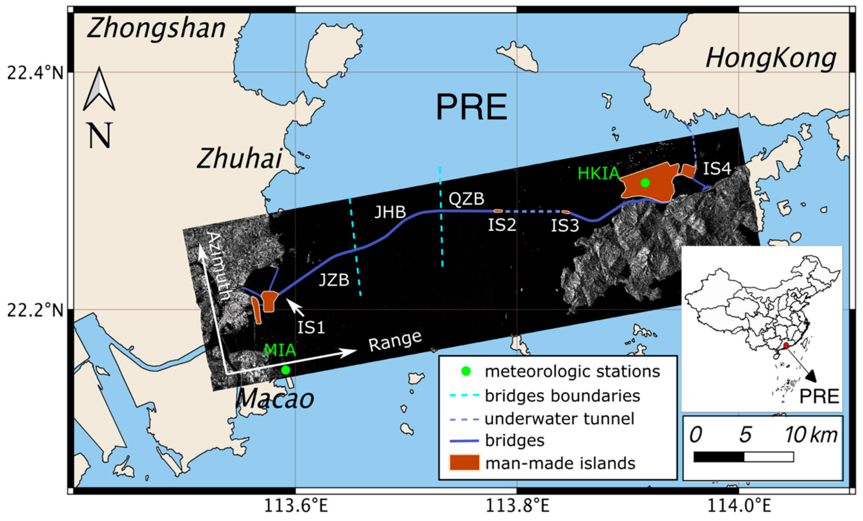
2.1. Study Area
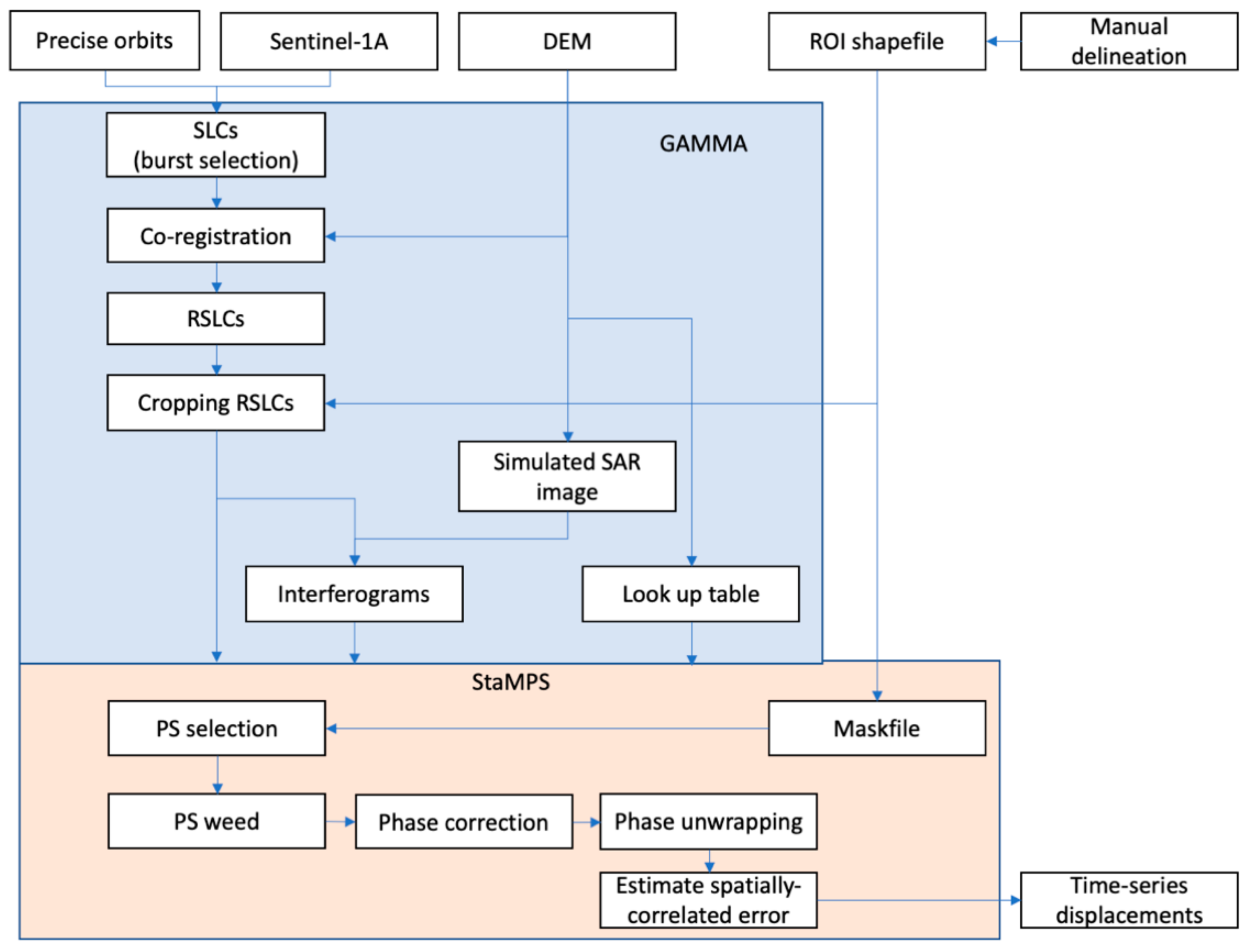
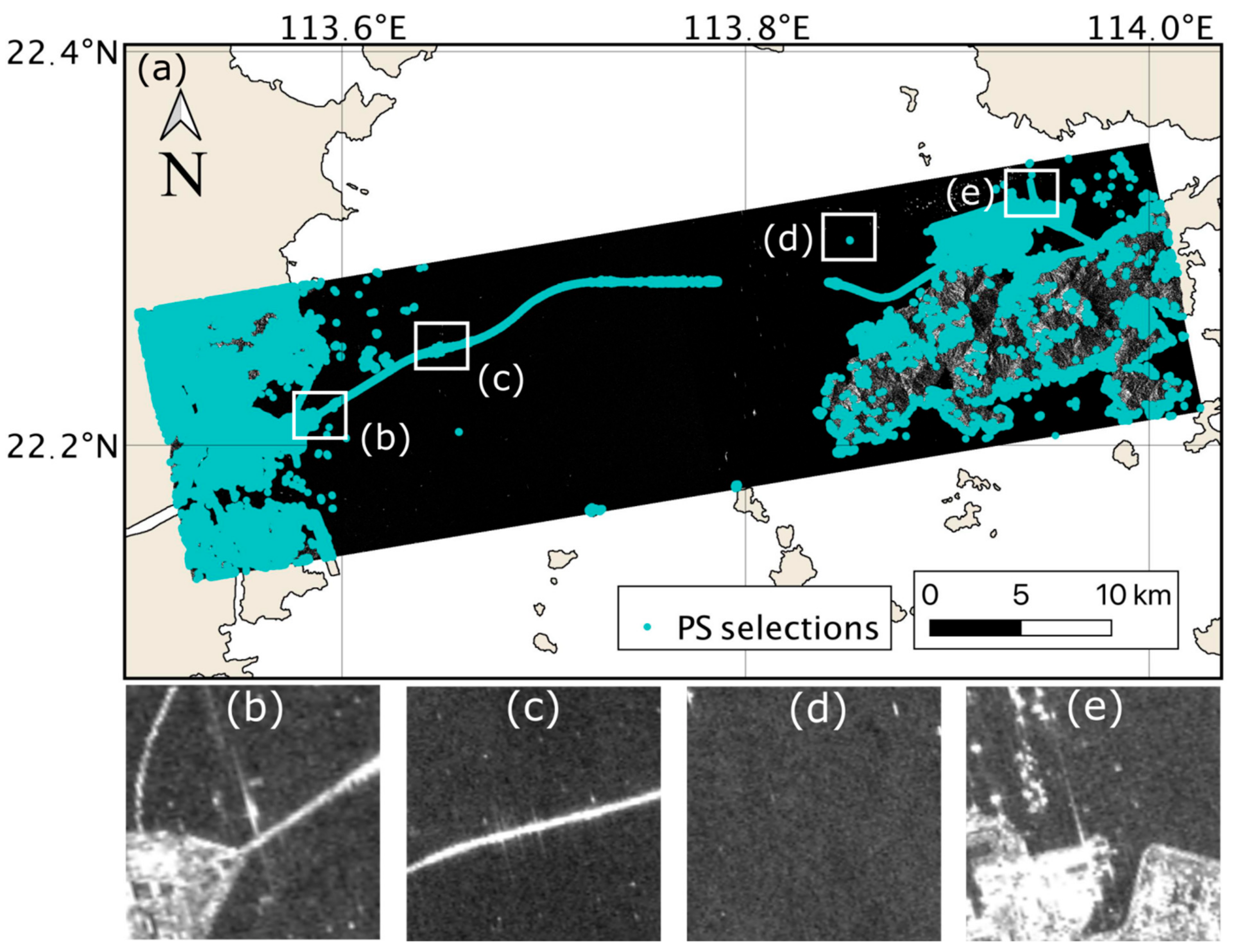
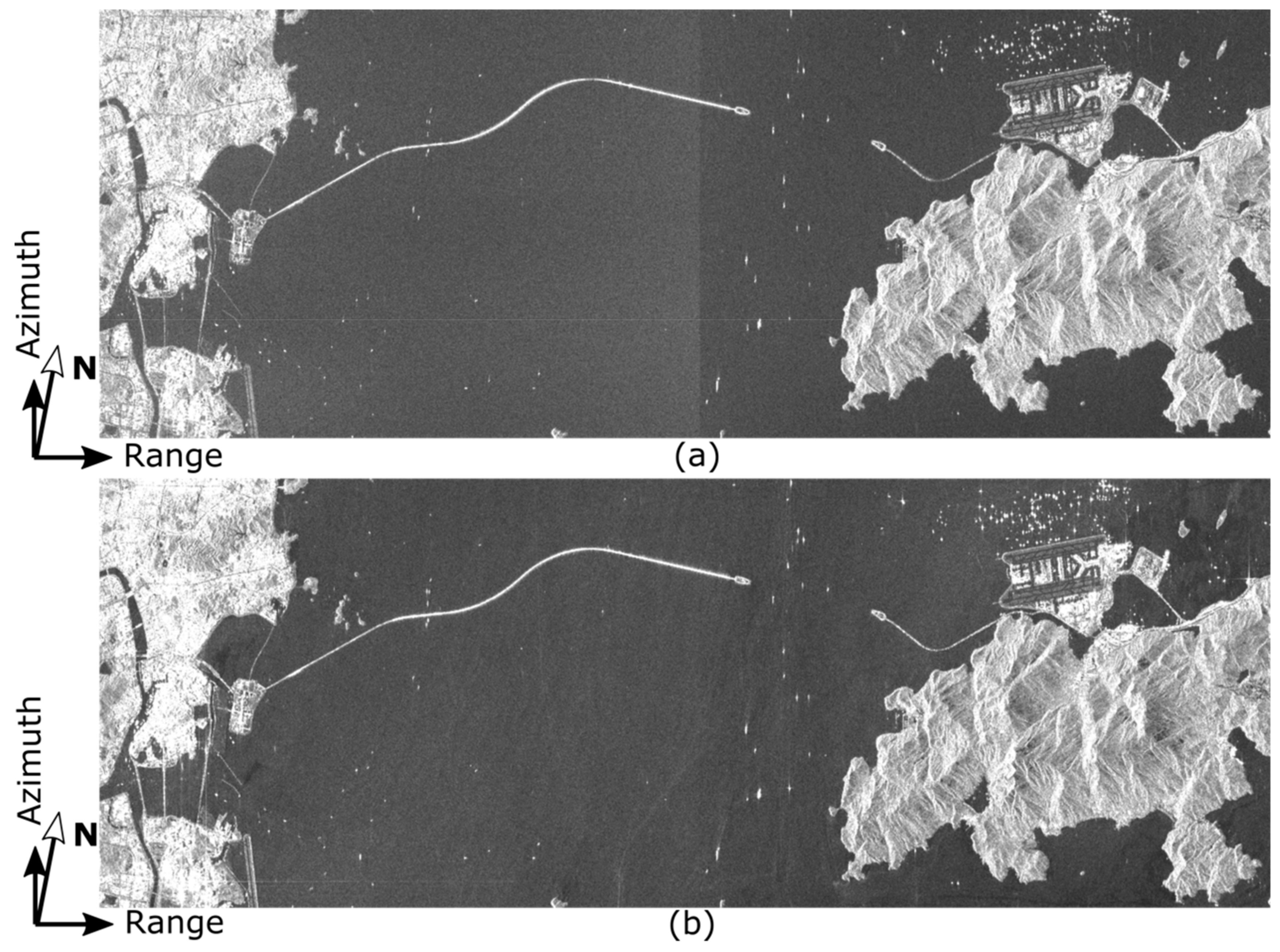
2.2. PS-InSAR Processing Based on GAMMA and Stanford Method for Persistent Scatterers (StaMPS)
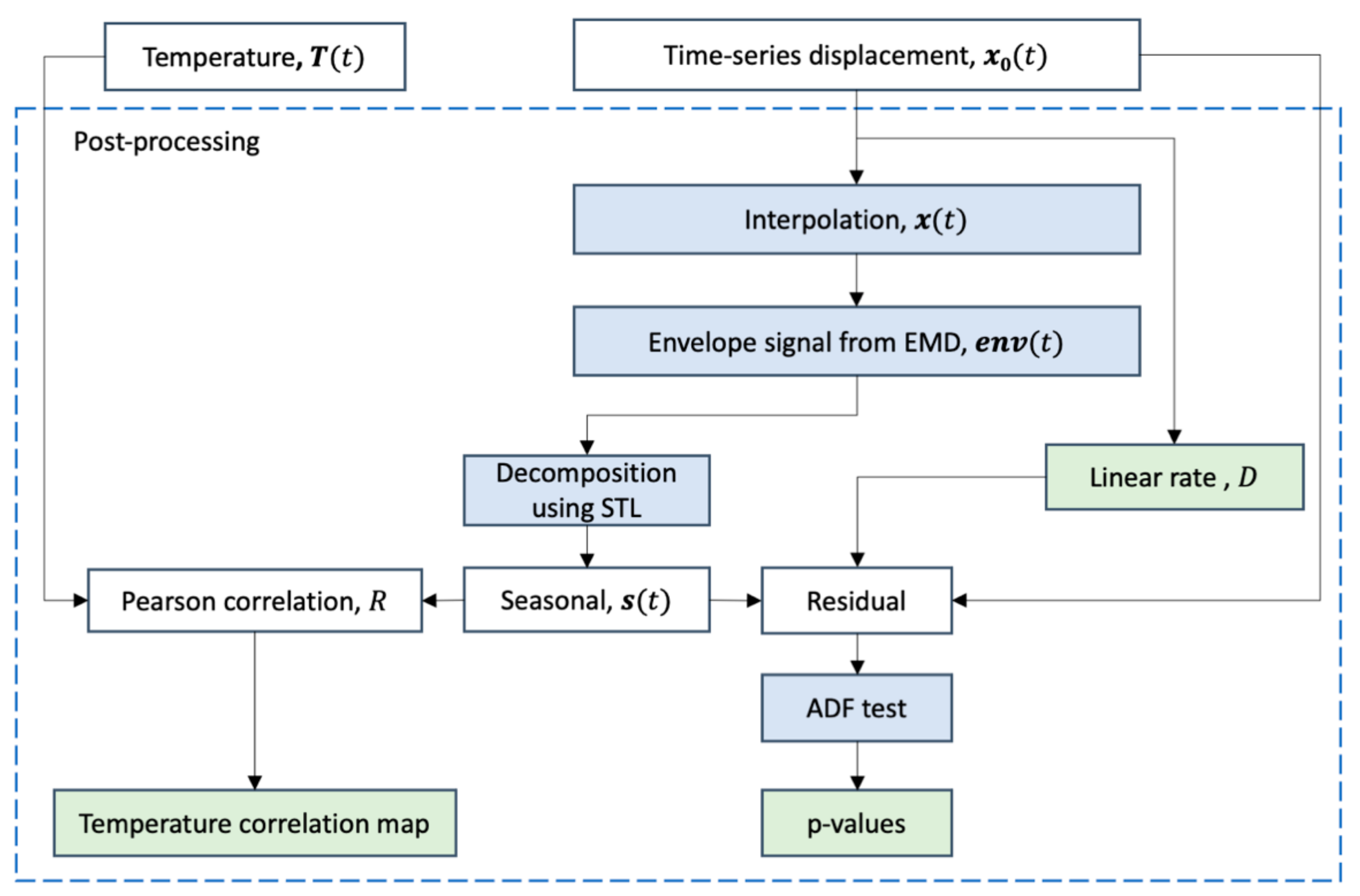
2.3. Post-Processing Based on Time-Series Analysis
2.3.1. Interpolation and Linear Fit
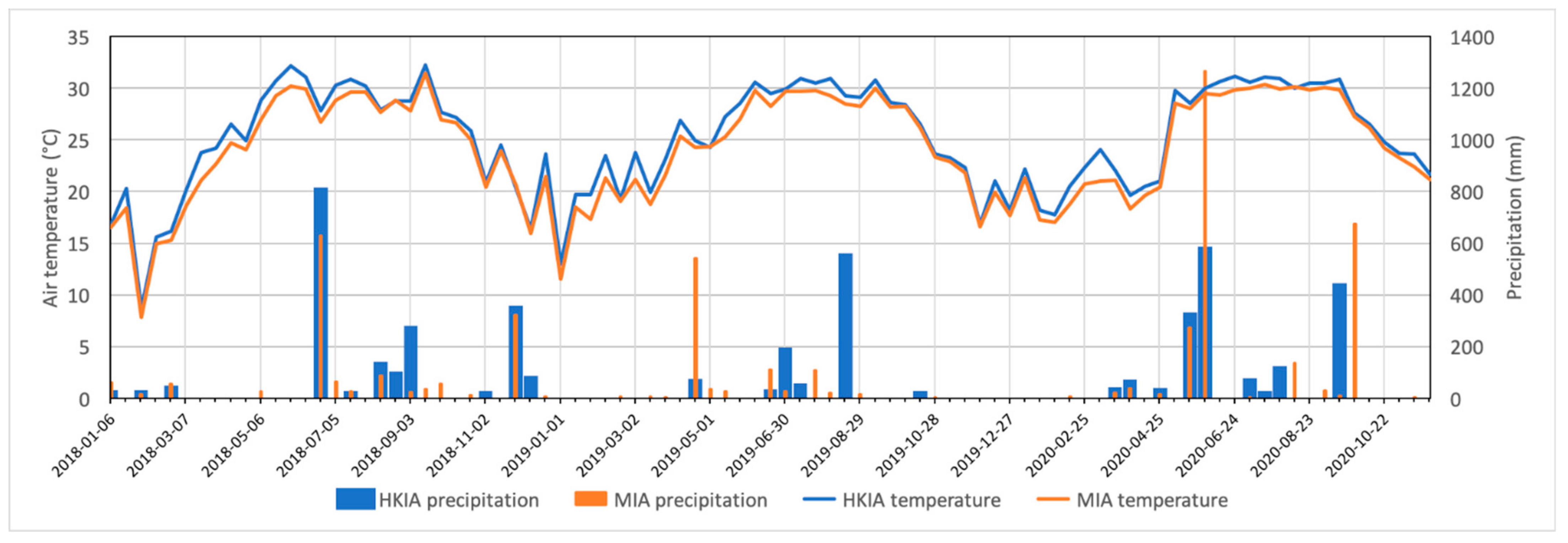
2.3.2. Temperature Correlation Based on EMD and STL
2.3.3. Irregular Variation Detected by ADF Test
3. Results
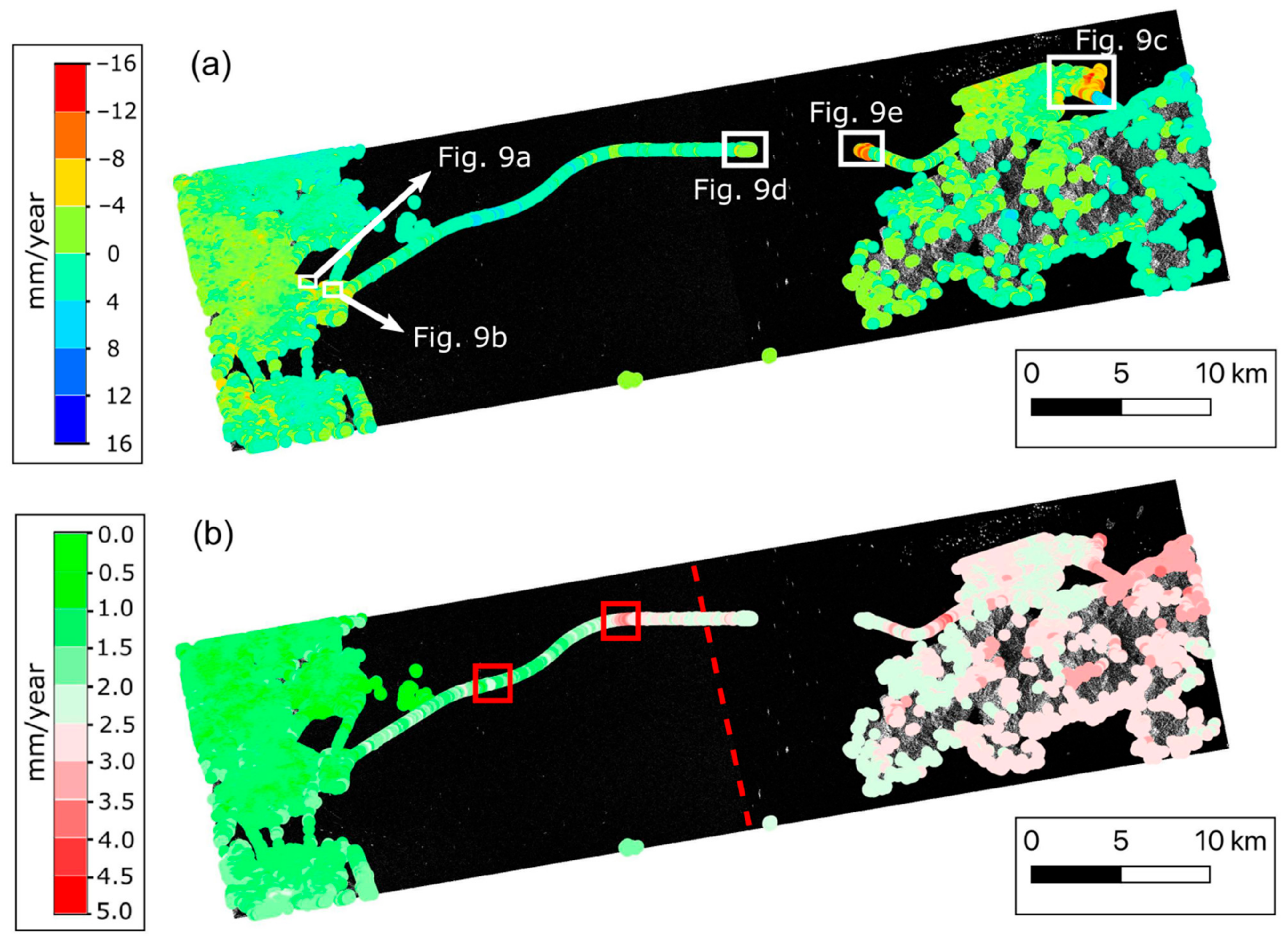
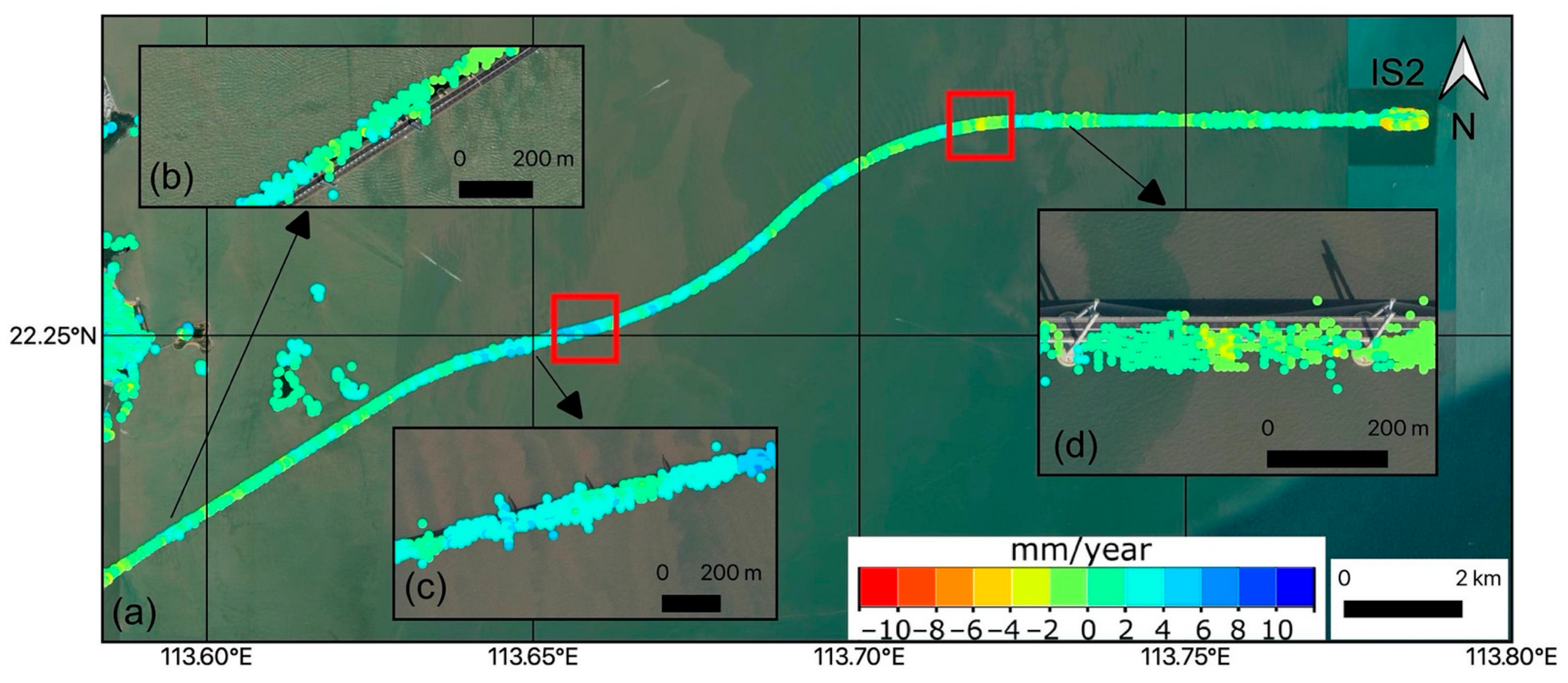
3.1. InSAR-Derived Time-Series Displacements
3.2. Post-Processing Based on Time-Series Analysis
4. Discussion
5. Conclusions
Author Contributions
Funding
Institutional Review Board Statement
Informed Consent Statement
Data Availability Statement
Acknowledgments
Conflicts of Interest
References
- The State-of-the-Practice of Modern Structural Health Monitoring for Bridges: A Comprehensive Review. Available online: http://www.mtri.org/bridgecondition/doc/State-of-PracticeSHMforBridges(July2010).pdf (accessed on 3 February 2021).
- Omar, T.; Nehdi, M.L. Remote sensing of concrete bridges decks using unmanned aerial vehicle infrared thermography. Automat. Constr. 2017, 83, 360–371. [Google Scholar] [CrossRef]
- Liu, X.; Wang, P.; Lu, Z.; Gao, K.; Wang, H.; Jiao, C.; Zhang, X. Using terrestrial laser scanning (TLS), Ground-based microwave interferometry, and permanent scatterer interferometry synthetic aperture radar (PS-InSAR). Remote Sens. 2019, 11, 580. [Google Scholar] [CrossRef] [Green Version]
- Alani, A.M.; Aboutalebi, M.; Kilic, G. Applications of ground penetrating radar (GPR) in bridge deck monitoring and assessment. J. Appl. Geophys. 2013, 97, 45–54. [Google Scholar] [CrossRef]
- Meng, X.; Dodson, A.H.; Roberts, G.W. Detecting bridge dynamics with GPS and triaxial accelerometers. Eng. Struct. 2007, 29, 3178–3184. [Google Scholar] [CrossRef]
- Zhang, B.C.; Ding, X.L.; Werner, C.L.; Tan, K.; Zhang, B.; Jiang, M.; Zhao, J.W.; Xu, Y.L. Dynamic Displacement Monitoring of Long-Span Bridges with a Microwave Radar Interferometer. Isprs J. Photogramm. Remote Sens. 2018, 138, 252–264. [Google Scholar] [CrossRef]
- Lee, J.; Lee, K.C.; Lee, S.; Lee, Y.J.; Sim, S.H. Long-term displacement measurement of bridges using a LiDAR system. Struct. Control Health Monit. 2019, 26, 2428. [Google Scholar] [CrossRef]
- Sousa, J.J.; Bastos, L. Multi-temporal SAR interferometry reveals acceleration of bridge sinking before collapse. Nat. Hazards Earth Syst. Sci. Discuss. 2013, 13, 659–667. [Google Scholar] [CrossRef]
- Ferretti, A.; Prati, C.; Rocca, F. Nonlinear subsidence rate estimation using permanent scatterers in differential SAR interferometry. IEEE Trans. Geosci. Remote Sens. 2001, 38, 2202–2212. [Google Scholar] [CrossRef] [Green Version]
- Ferretti, A.; Prati, C.; Rocca, F. Permanent scatterer in SAR interferometry. IEEE Trans. Geosci. Remote Sens. 2001, 39, 8–20. [Google Scholar] [CrossRef]
- Berardino, P.; Fornaro, G.; Lanari, R.; Sansosti, E. A new algorithm for surface deformation monitoring based on small baseline differential SAR interferograms. IEEE Trans. Geosci. Remote Sens. 2002, 40, 2375–2384. [Google Scholar] [CrossRef] [Green Version]
- Sousa, J.J.; Hlavacova, I.; Bakon, M.; Lazecky, M.; Patricio, G.; Guimaraes, P.; Ruiz, A.M.; Bastos, L.; Sousa, A.; Bento, R. Potential of Multi-Temporal InSAR Techniques for Bridges and Dams Monitoring. Procedia Technol. 2014, 16, 834–841. [Google Scholar] [CrossRef] [Green Version]
- Milillo, P.; Giardina, G.; Perissin, D.; Milillo, G.; Coletta, A.; Terranova, C. Pre-collapse space geodetic observations of critical infrastructure: The Morandi Bridge, Genoa, Italy. Remote Sens. 2019, 11, 1403. [Google Scholar] [CrossRef] [Green Version]
- Milillo, P.; Giardina, G.; DeJong, M.J.; Perissin, D.; Milillo, G. Multi-temporal InSAR structural damage assessment: The London Crossrail case study. Remote Sens. 2019, 10, 287. [Google Scholar] [CrossRef] [Green Version]
- Owerko, T.; Kuras, P. Effective processing of radar data for bridge damage detection. Hindawi Shock Vib. 2019. [Google Scholar] [CrossRef]
- Selvakumaran, S.; Plank, S.; Geiß, C.; Rossi, C.; Middleton, C. Remote monitoring to predict bridge scour failure using Interferometric synthetic aperture radar (InSAR) stacking techniques. Int. J. Appl. Earth Obs. Geoinf. 2018. [Google Scholar] [CrossRef]
- Niu, F.; Liu, M.; Cheng, G.; Lin, Z.; Luo, J.; Yin, G. Long-term thermal regimes of the Qinghai-Tibet railway embankments in plateau permafrost regions. Sci. China Earth Sci. 2015, 58, 1669–1676. [Google Scholar] [CrossRef]
- Ma, P.; Li, T.; Fang, C.; Lin, H. A tentative test for measuring the sub-millimeter settlement and uplift of a high-speed railway bridge using COSMO-SkyMed images. Isprs J. Photogramm. Remote Sens. 2019. [Google Scholar] [CrossRef]
- Qin, X.; Liao, M.; Zhang, L.; Yang, M. Structural health and stability assessment of high-speed railways via thermal dilation mapping with time-series InSAR analysis. IEEE J. Sel. Top. Appl. Earth Obs. Remote Sens. 2017, 10, 2999–3010. [Google Scholar] [CrossRef] [Green Version]
- Qin, X.; Zhang, L.; Yang, M.; Luo, H.; Liao, M.; Ding, X. Mapping surface deformation and thermal dilation of arch bridges by structure-driven multi-temporal DInSAR analysis. Remote Sens. Environ. 2019. [Google Scholar] [CrossRef]
- Zhang, L.; Sun, Q.; Hu, J. Potential of TCPInSAR in Monitoring Linear Infrastructure with a Small Dataset of SAR Images: Application of the Donghai Bridge, China. Appl. Sci. 2018, 8, 425. [Google Scholar] [CrossRef] [Green Version]
- Wang, H.; Chang, L.; Markine, V. Structural health monitoring of railway transition zones using satellite radar data. Sensors 2019, 18, 413. [Google Scholar] [CrossRef] [PubMed] [Green Version]
- Monserrat, O.; Crosetto, M.; Cuevas, M.; Crippa, B. The thermal expansion component of persistent scatterer interferometry observations. IEEE Geosci. Remote Sens. Lett. 2011, 8, 864–867. [Google Scholar] [CrossRef]
- Chang, L. Monitoring Civil Infrastructure Using Satellite Radar Interferometry. Ph.D. Thesis, Delft University of Technology, Delft, The Netherlands, July 2015. [Google Scholar]
- Wu, S.B.; Yang, Z.F.; Ding, X.L.; Zhang, B.C.; Zhang, L.; Lu, Z. Two Decades of Settlement of Hong Kong International Airport Measured with Multi-Temporal InSAR. Remote Sens. Environ. 2020. [Google Scholar] [CrossRef]
- Lyu, M.; Ke, Y.; Li, X.; Zhu, L.; Guo, L.; Gong, H. Detection of seasonal deformation of highway overpasses using the PS-InSAR technique: A case study in Beijing urban area. Remote Sens. 2020, 12, 3071. [Google Scholar] [CrossRef]
- Zhu, M.; Wan, X.; Fei, B.; Qiao, Z.; Ge, C.; Minati, F.; Vecchioli, F.; Li, J.; Costantini, M. Detection of building and infrastructure instabilities by automatic spatiotemporal analysis of satellite SAR interferometry measurements. Remote Sens. 2018, 10, 1816. [Google Scholar] [CrossRef] [Green Version]
- Hu, Z.; Xie, Y.; Wang, J. Challenges and strategies involved in designing and constructing a 6 km immersed tunnel: A case study of the Hong Kong–Zhuhai–Macao Bridge. Tunn. Undergr. Space Technol. 2015, 50, 171–177. [Google Scholar] [CrossRef]
- Gao, W.; Su, Q.; Zhang, J.; Xie, H.; Wen, F.; Li, F.; Liu, J. Steel Bridge Construction of Hong Kong–Zhuhai–Macao Bridge. Int. J. Steel Struct. 2020, 20, 1498–1508. [Google Scholar] [CrossRef]
- Wegnüller, U.; Werner, C.; Strozzi, T.; Wiesmann, A.; Frey, O.; Santoro, M. Sentinel-1 support in the GAMMA software. Procedia Comput. Sci. 2016, 100, 1305–1312. [Google Scholar] [CrossRef] [Green Version]
- Hooper, A.; Zebker, H.; Segall, P.; Kampes, B. A new method for measuring deformation on volcanoes and other natural terrains using InSAR persistent scatterers. Geophys. Res. Lett. 2004, 31, L23611. [Google Scholar] [CrossRef]
- Huang, N.E.; Shen, Z.; Long, S.R.; Wu, M.C.; Shih, H.H.; Zheng, Q.; Yen, N.-C.; Tung, C.C.; Liu, H.H. The empirical mode decomposition and the Hilbert spectrum for nonlinear and non-stationary time series analysis. Proc. R. Soc. Lond. A 1998, 454, 903–995. [Google Scholar] [CrossRef]
- Cleveland, R.B.; Cleveland, W.S.; McRae, J.E.; Terpenning, I. STL: A seasonal-trend decomposition. J. Off. Stat. 1990, 6, 3–73. [Google Scholar]
- Global Surface Summary of the Day—GSOD, the National Oceanic and Atmospheric Administration (NOAA). Available online: https://www.ncei.noaa.gov/metadata/geoportal/rest/metadata/item/gov.noaa.ncdc:C00516/html (accessed on 21 January 2021).
- Fuller, W.A. Introduction to Statistical Time Series; John Wiley and Sons: New York, NY, USA, 1976; ISBN 0-471-28715-6. [Google Scholar]
- Lopez, J.H. The power of the ADF test. Econ. Lett. 1997, 57, 5–10. [Google Scholar] [CrossRef]


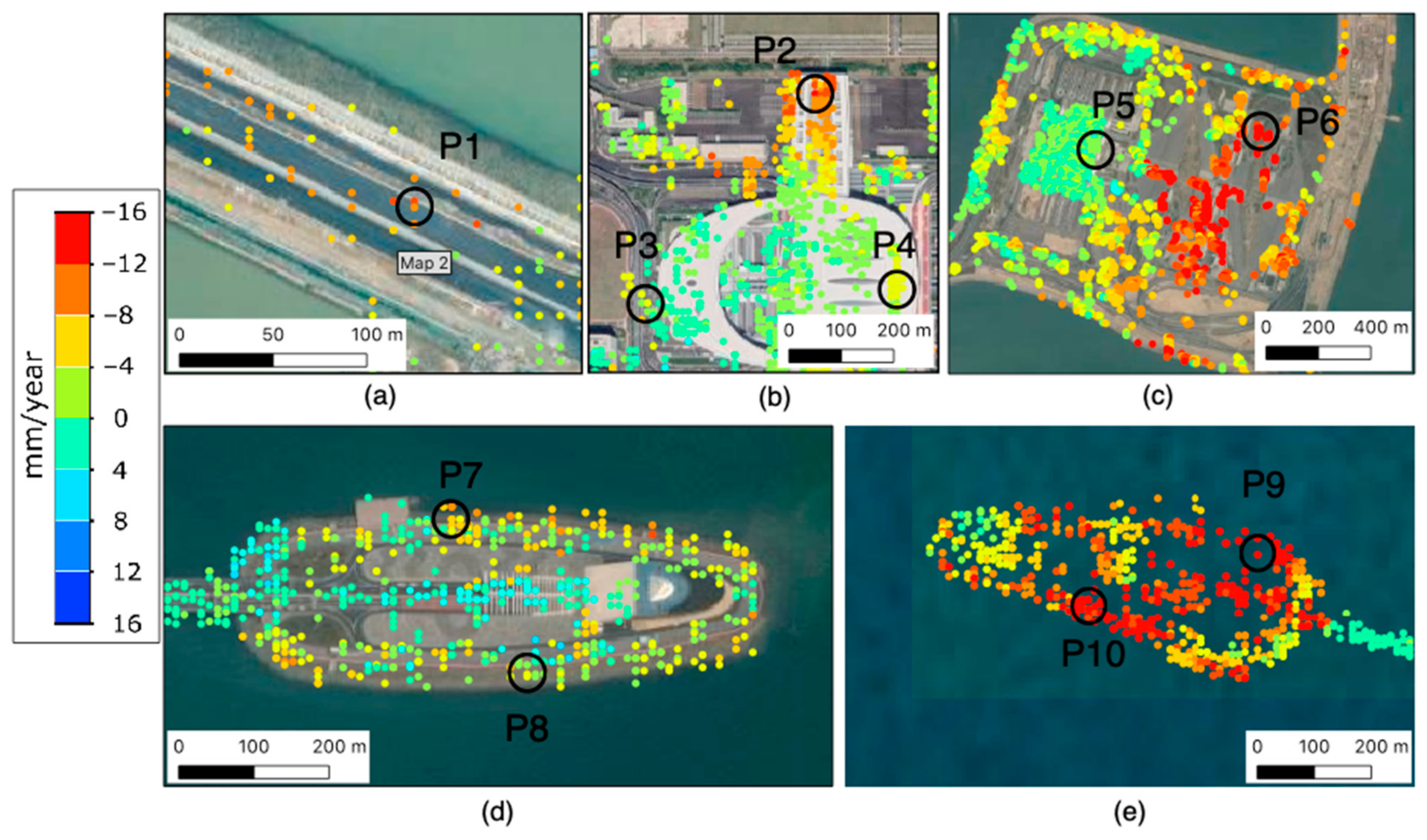
| Label | No. | Latitude (Degree) | Longitude (Degree) | Linear rate (mm/Year) | R | Description |
|---|---|---|---|---|---|---|
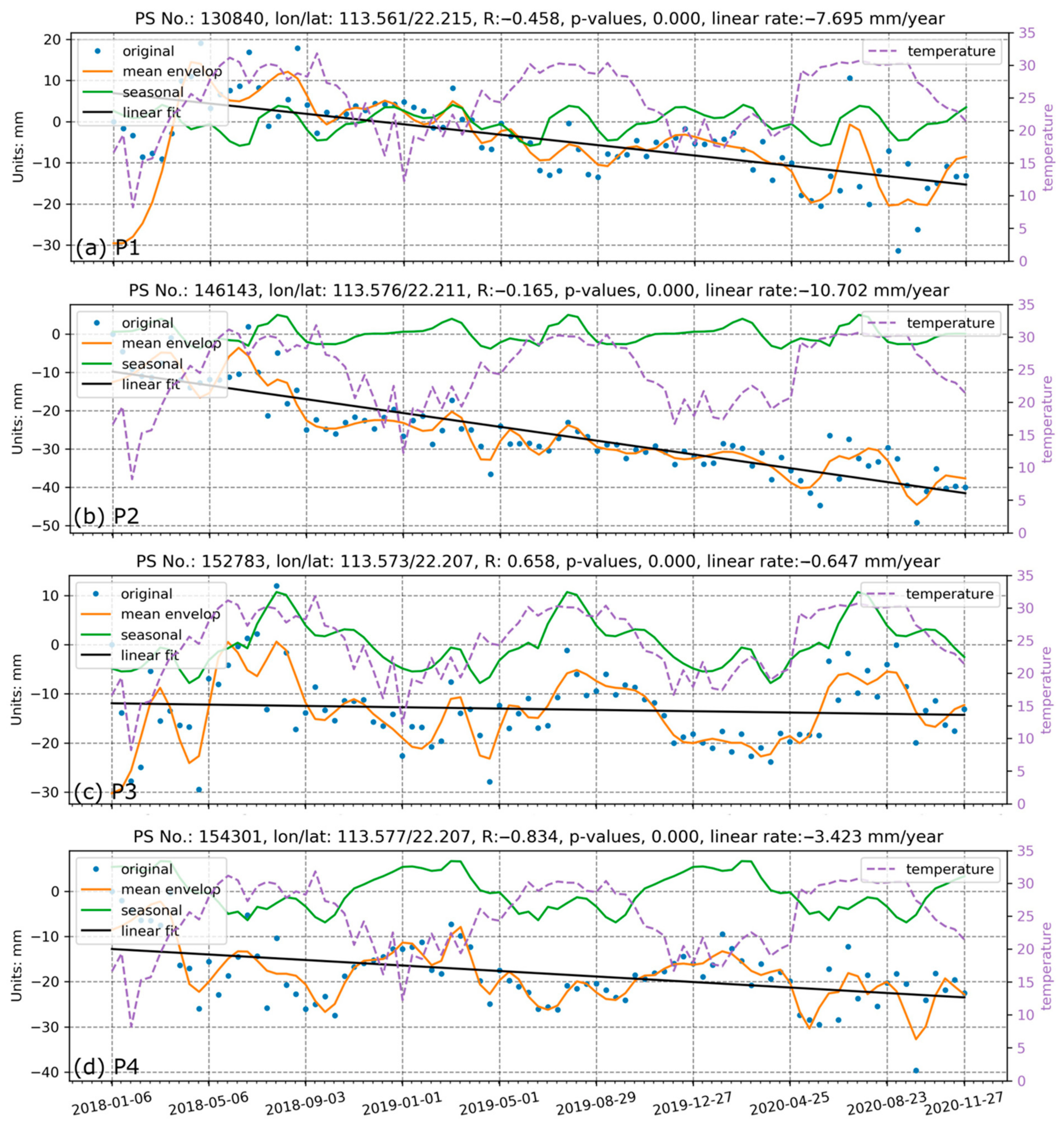
| P1 | 130840 | 113.5612 | 22.2150 | −7.6953 | −0.4585 | Bridge from Zhuhai city to Zhuhai Terminal |
| P2 | 146143 | 113.5759 | 22.2107 | −10.7019 | −0.1649 | Northern cloister of Zhuhai Passenger Terminal |
| P3 | 152783 | 113.5730 | 22.2071 | −0.6469 | 0.6580 | Back of the Zhuhai Passenger Terminal |
| P4 | 154301 | 113.5773 | 22.2074 | −3.4231 | −0.8345 | Front of the Zhuhai Passenger Terminal |
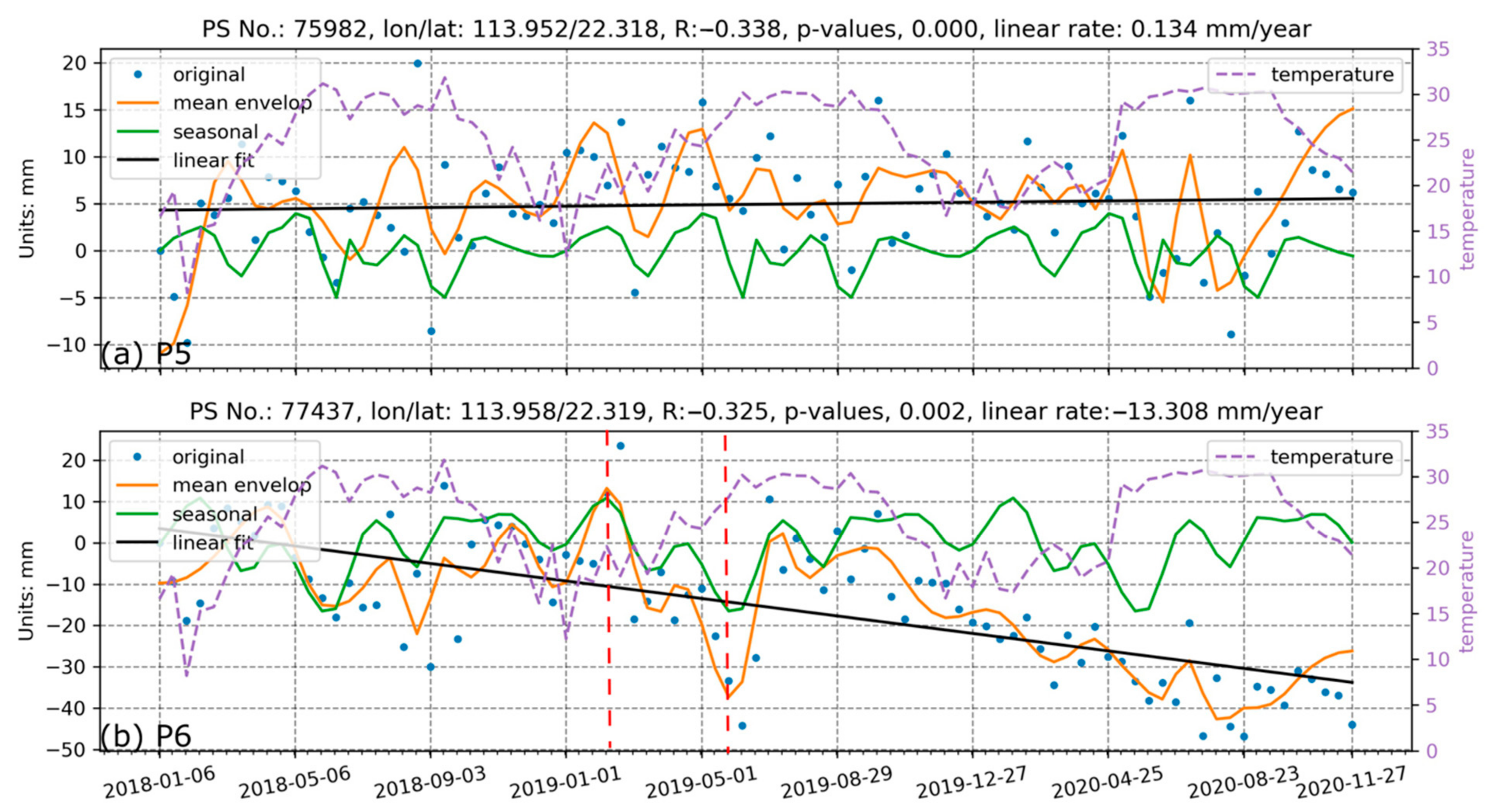
| P5 | 75982 | 113.9519 | 22.3180 | 0.1343 | −0.3382 | East side of the Hong Kong Terminal |
| P6 | 77437 | 113.9577 | 22.3186 | −13.3084 | −0.3245 | A small building |
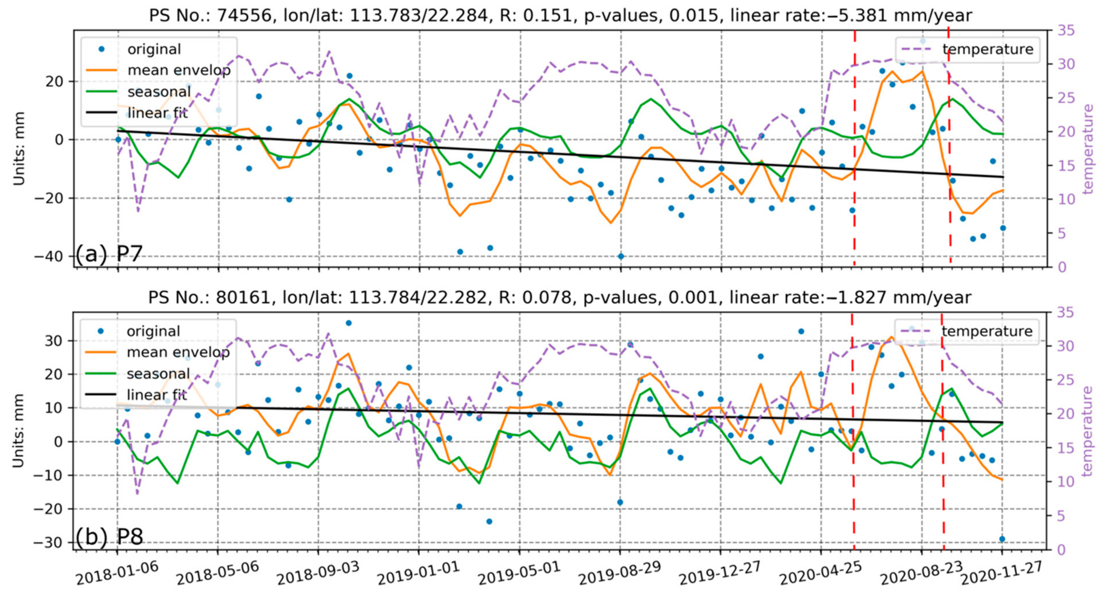
| P7 | 74556 | 113.7829 | 22.2841 | −5.3813 | 0.1513 | North of the west man-made island |
| P8 | 80161 | 113.7838 | 22.2822 | −1.8265 | 0.0781 | South of the west man-made island |
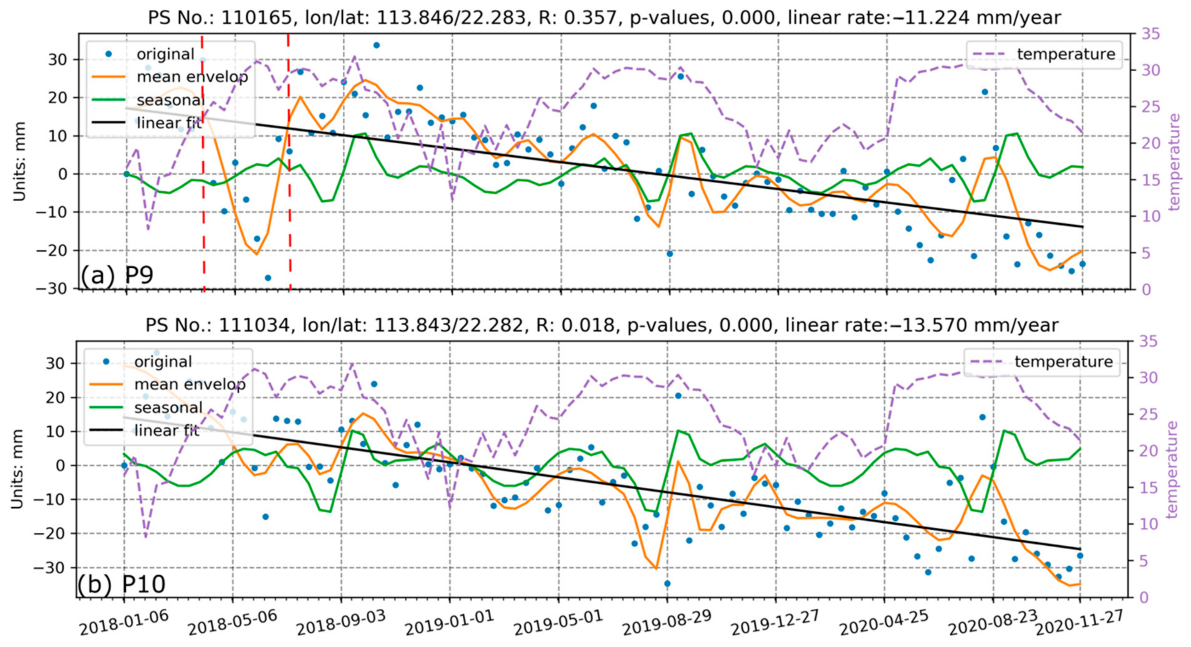
| P9 | 110165 | 113.8458 | 22.2826 | −11.2244 | 0.3566 | Northeast of the east man-made island |
| P10 | 111034 | 113.8432 | 22.2817 | −13.5703 | 0.0177 | South of the east man-made island |
Publisher’s Note: MDPI stays neutral with regard to jurisdictional claims in published maps and institutional affiliations. |
© 2021 by the authors. Licensee MDPI, Basel, Switzerland. This article is an open access article distributed under the terms and conditions of the Creative Commons Attribution (CC BY) license (http://creativecommons.org/licenses/by/4.0/).
Share and Cite
Xiong, S.; Wang, C.; Qin, X.; Zhang, B.; Li, Q. Time-Series Analysis on Persistent Scatter-Interferometric Synthetic Aperture Radar (PS-InSAR) Derived Displacements of the Hong Kong–Zhuhai–Macao Bridge (HZMB) from Sentinel-1A Observations. Remote Sens. 2021, 13, 546. https://0-doi-org.brum.beds.ac.uk/10.3390/rs13040546
Xiong S, Wang C, Qin X, Zhang B, Li Q. Time-Series Analysis on Persistent Scatter-Interferometric Synthetic Aperture Radar (PS-InSAR) Derived Displacements of the Hong Kong–Zhuhai–Macao Bridge (HZMB) from Sentinel-1A Observations. Remote Sensing. 2021; 13(4):546. https://0-doi-org.brum.beds.ac.uk/10.3390/rs13040546
Chicago/Turabian StyleXiong, Siting, Chisheng Wang, Xiaoqiong Qin, Bochen Zhang, and Qingquan Li. 2021. "Time-Series Analysis on Persistent Scatter-Interferometric Synthetic Aperture Radar (PS-InSAR) Derived Displacements of the Hong Kong–Zhuhai–Macao Bridge (HZMB) from Sentinel-1A Observations" Remote Sensing 13, no. 4: 546. https://0-doi-org.brum.beds.ac.uk/10.3390/rs13040546