Landsat 8 Thermal Infrared Sensor Scene Select Mechanism Open Loop Operations


1
U.S. Geological Survey, Earth Resources Observation and Science Center, Sioux Falls, SD 57030, USA
2
KBR, Contractor to the U.S. Geological Survey, Earth Resources Observation and Science Center, Sioux Falls, SD 57030, USA
*
Author to whom correspondence should be addressed.
Remote Sens. 2021, 13(4), 617; https://0-doi-org.brum.beds.ac.uk/10.3390/rs13040617
Submission received: 24 November 2020
/
Revised: 13 January 2021
/
Accepted: 21 January 2021
/
Published: 9 February 2021
(This article belongs to the Special Issue Cross-Calibration and Interoperability of Remote Sensing Instruments)
Abstract
:The Landsat 8 (L8) spacecraft and its two instruments, the operational land imager (OLI) and thermal infrared sensor (TIRS), have been consistently characterized and calibrated since its launch in February 2013. These performance metrics and calibration updates are determined through the U.S. Geological Survey (USGS) Landsat image assessment system (IAS), which has been performing this function since its launch. The TIRS on-orbit geometric calibration procedures include TIRS-to-OLI alignment, TIRS sensor chip assembly (SCA) alignment, and TIRS band alignment. In December 2014, the TIRS instrument experienced an anomalous condition related to the instrument’s ability to accurately measure the location of the scene select mechanism (SSM). The SSM is a rotating mirror that allows the instrument’s field of view to be pointed at the Earth, for normal imaging, or at either deep space or an onboard black body, for radiometric calibration purposes. This anomalous condition in the SSM’s position sensor made it necessary to implement a new mode of operation for this mirror, termed mode-0. Mode-0 involves operating the mirror in an open-loop control state during normal mission operations when acquiring Earth data. Closed-loop mode-4 is needed for directing the mirror towards the radiometric calibration targets and is used approximately once every two weeks to collect radiometric calibration data. Mode-0 is used for most operational imaging because it does not require SSM encoder data, thereby allowing the SSM encoder electronics to remain unpowered most of the time, reducing its use throughout the lifetime of the TIRS instrument, thus helping to preserve its nominal behavior during it use. This paper discusses the geometric calibration of the SSM mirror during its current normal mode-0 set of image operations, as its open-loop control allows the mirror to drift over time in its uncontrolled state and its effects on products. The results shown in this paper demonstrate that the ability to have ongoing updates to the modeling of the TIRS SSM mirror model, in both an automated fashion and with a set of more manual operations, allows accuracy that approaches mode-4 results within days from the start of a mode-0 event.
1. Introduction
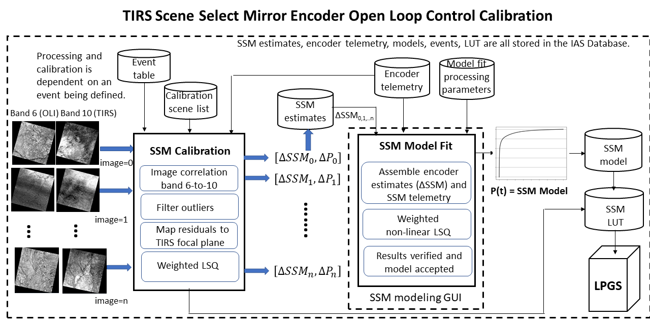
The Landsat 8 (L8) spacecraft was launched on 11 February, 2013 [1,2,3]. This spacecraft is a continuation of the Landsat program, whose mission is to provide 16-day global coverage of the Earth’s landmass with the purpose of providing high-quality science grade imagery to the user community. The spacecraft carries two payloads, the operational land imager (OLI) [4] and the thermal infrared sensor (TIRS) [5]. The TIRS instrument contains two thermal bands (10.6–11.2 µm and 11.5–12.5 µm), labeled as band 10 and band 11, respectively. These bands are made up of quantum well infrared photodetectors (QWIP) assembled on three sensor chip assemblies (SCAs) within the focal plane, each covering approximately one-third of the full 185-km field of view. The two spectral bands have a nominal ground sampling distance (GSD) of 100 m. The co-alignment between the TIRS and OLI instruments is required to be within 7 milliradians, and the TIRS field of view is required to be contained within the (larger) field of view of the OLI instrument. An L8 three-band image using OLI and TIRS bands, with all three bands resampled to a 30-m pixel size, is shown in Figure 1. Using a combination of bands 10 (TIRS), 7 (OLI), and 2 (OLI) helps to delineate the two fields of view within the image. From Figure 1, it can be seen that the TIRS instrument’s east and west edges are within the OLI instrument’s east and west edges.
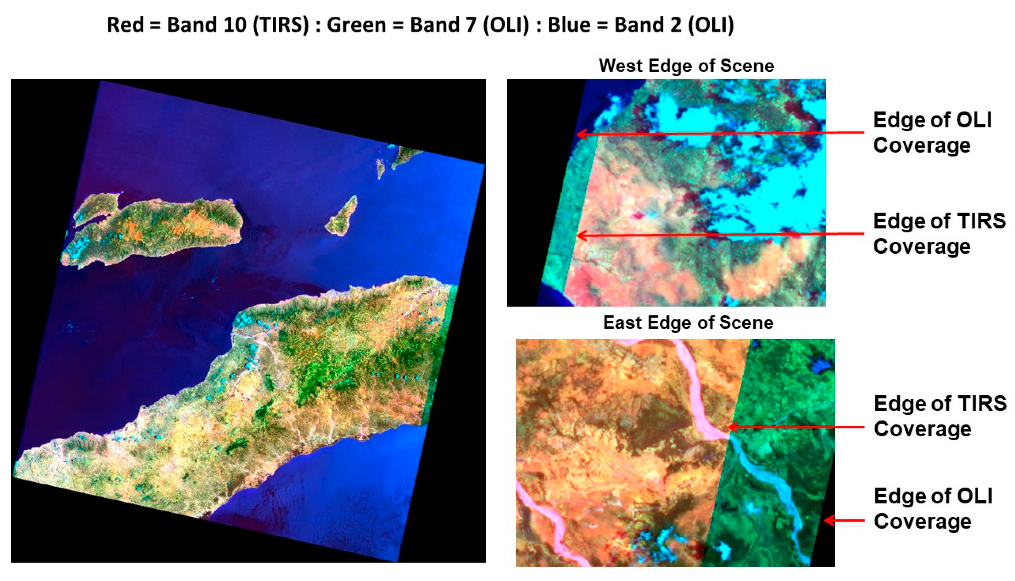
In order to support on-orbit radiometric calibration, a movable scene select mirror (SSM) is positioned in front of the TIRS telescope to direct the field of view of the focal plane to the two radiometric calibration sources. Therefore, including Earth collections, there are three positions of the SSM, toward Earth and toward the two radiometric calibration sources, deep space and the onboard black body. Both deep space and the black body are imaged for approximately 30 s during a radiometric calibration operation. The deep space collection and black body collections provide measurements of the instrument’s bias, and performance against a known target, respectively. The SSM encoder provides the required high degree of accuracy in position knowledge of the SSM needed for positioning the mirror for each collection, ensuring that the pointing accuracy of TIRS is met for each of these three types of collects. A cutaway of the TIRS instrument is shown in Figure 2. Details of the SSM are shown on the right side of the figure, while the left side shows the SSM assembly on top of the telescope/focal plane assembly (FPA) in the integrated TIRS instrument.
The original operational concept for the TIRS instrument was to perform both radiometric collects, deep space and black body, twice per orbit. The Landsat 8 (L8) image assessment system (IAS), developed, built and maintained by the U.S. Geological Survey (USGS) in collaboration with the National Aeronautics and Space Administration (NASA), performs characterization and calibration of the spacecraft and instruments onboard the L8 satellite. The IAS is designed to automatically reduce the deep space, and black body collects to produce TIRS radiometric calibration parameters that are applied to the Earth-view collects between calibrations. The data acquired in the mode-0 and mode-4 set of operations from a user’s perspective is radiometrically equivalent. Specifics on the radiometric stability of the TIRS instrument can be found in [6].
On 19 December, 2014, anomalous current levels were detected on the primary side-A electronics associated with the SSM encoder electronics. Investigations and analysis led to the switch from the primary A-side to the redundant B-side TIRS mechanism control electronics (MCE). This switch occurred on 2 March 2015. In late October of 2015, the L8 flight operations team (FOT) observed an upward increasing trend in the B-side encoder electronics current followed by an anomalous condition associated with the instrument’s ability to measure the location of the SSM on 2 November 2015. The anomalous behavior exhibited by the redundant encoder electronics brought about the need to develop a method of operations that limited the use of the SSM encoder electronics. This involved the use of the SSM in an open-loop/uncontrolled state of motion without powering the SSM motor and allows the mirror to drift over time, which is referred to in this article as TIRS SSM mode-0 operations. Nominal closed-loop/controlled operations, prior to the implementation of mode-0, were termed as mode-4 operations and involved powering the mirror within a controlled state. The revised SSM operations concept is thus to switch the SSM into mode-4 for a radiometric calibration operation approximately twice per month (with one calibration operation coinciding with an OLI lunar calibration operation) but to leave the SSM in mode-0 for normal Earth-imaging between these radiometric calibration maneuvers. To provide SSM position knowledge immediately following each radiometric calibration maneuver, after switching from the closed-loop (mode-4) to mode-0, the SSM encoder is left on for several orbits. The time and duration of leaving the SSM encoder on depends on several factors such as the radiometric calibration type (e.g., lunar), so each mode-0 “event” begins with accurate position knowledge provided by the encoder. Subsequent SSM position information must be estimated from the imagery.
The TIRS SSM geometric calibration and modeling algorithm details, including the mathematical equations involved, are summarized here but can be found in more detail in other documents [7]. This document focuses on the processes involved that would be of most interest to the user community with regard to the impact on their products.
2. Methods
During the TIRS SSM anomaly investigation, it was experimentally determined that when the SSM is switched to mode-0 and released from closed-loop control, the SSM reacts to the residual magnetic torque in the motor by moving rapidly at first and then transitioning to a slower decaying rate, away from the chosen starting nadir position. It was found that the magnitude and variability of this post-switch motion can be reduced by applying decreasing-sized motor motions in alternate directions prior to releasing the SSM. This so-called “pendulum” maneuver is the operational implementation of the mode-4 (closed-loop) to mode-0 (open-loop) switch during imaging of the TIRS instruments as it is returned to its Earth viewing position. Because the Earth collects are imaged in open-loop control, without powering the SSM motor, specially developed algorithms are used to estimate the position of the SSM mirror from the TIRS images to accurately point the TIRS instrument to ensure that the products meet the TIRS-to-OLI band registration and geometric accuracy requirements.
Individual scene-based encoder estimates are measured using the TIRS-to-OLI alignment algorithm, which determines the alignment between the two instruments. For determining TIRS to OLI offsets, band 6 (OLI) is measured against band 10 (TIRS). All geometric algorithms within the IAS use the OLI Pan band as a geometric reference to which all other bands and SCAs are calibrated, using a series of algorithms including OLI Pan band SCA alignment, OLI to attitude control system (ACS) alignment, OLI between band registration, and finally sensor-to-sensor OLI-to-TIRS calibration alignment.
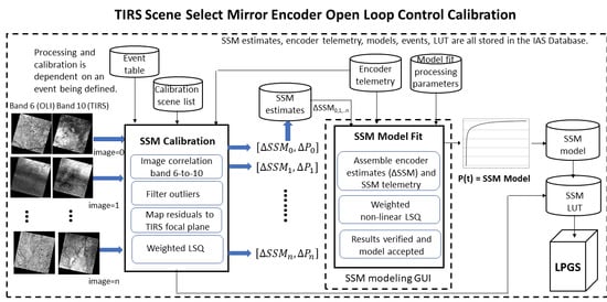
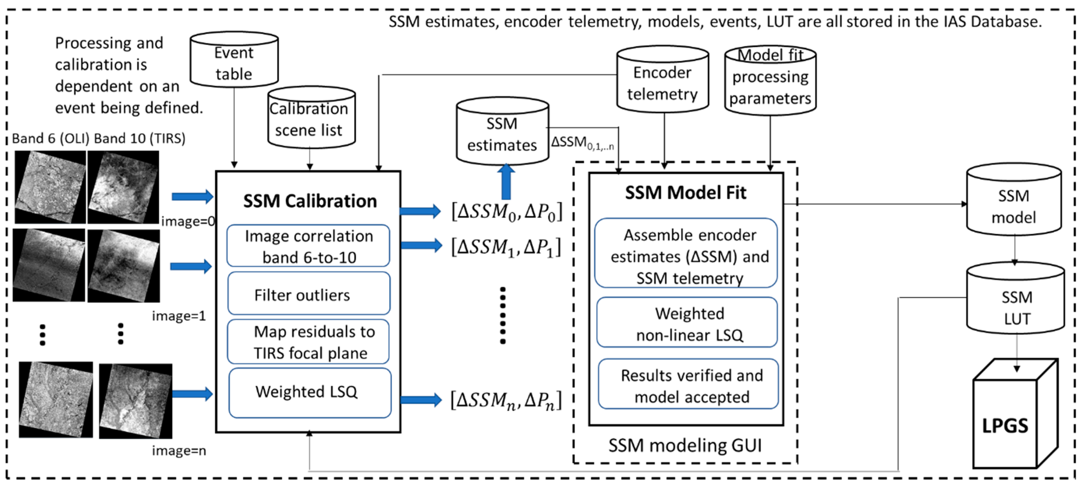
The TIRS SSM geometric calibration involves several steps. The scene-based measurement algorithm itself is a simpler version of the TIRS alignment algorithm. The TIRS alignment algorithm determines the alignment matrix with respect to the two instruments, TIRS and OLI, aboard the spacecraft. By determining the alignment between the TIRS and OLI instruments, where the OLI instrument is well-calibrated, the TIRS instrument can, in turn, be aligned with the spacecraft ACS indirectly, creating a sensor alignment between the TIRS instrument, the OLI instrument and spacecraft’s navigation system. For SSM geometric calibration, the alignment parameters are reduced to SSM positions, which impact the roll and yaw axes—the pitch component is not affected by changes in the SSM position. The TIRS SSM geometric calibration, therefore, estimates SSM positions based on differences in the alignment between the OLI and TIRS instruments. The estimated SSM positions over time are used to fit a time-dependent exponential model, referred to as the SSM model. The SSM model fit algorithm uses a combination of the encoder telemetry collected following the switch to mode-0 and the SSM position estimates from the image collects to fit a time-varying model of the SSM mirror position. The model used to determine the SSM position consists of both a linear and exponential component to the equation whose quality of fit is based on the time density of the encoder data acquired early in the mode-0 event and the ability to measure the movement of the mirror based on a set of geometric calibration sites during the SSM’s open-loop control period of operation. The steps involved in defining a given event and the SSM model include an initial model, which is the best estimate of the behavior absent any encoder related information, modifying the model’s behavior based on both actual encoder telemetry and the geometric calibration scene estimates, and determining a lookup table of the model’s equation. This determination of a look-up-table allows for an efficient creation of the geometric model needed for product generation. The geometric model is a file created during product generation that is used for mapping between geometrically raw but radiometrically calibrated pixels to map-projected image space. The steps in building the SSM model are outlined in the graphics in Figure 3.
2.1. SSM Model Fitting
2.1.1. SSM Model
The SSM model equation is shown below and includes an initial position offset, a position rate/slope parameter, and three decaying exponential terms with time constants varying from a few minutes to several days.
where:
P(t) = SSM position offset from nominal nadir position (in encoder counts) as a function of time from switch to mode-0 (t). The time is shown in units of both seconds and days to simplify the presentation of the equation by hiding the conversion factors.
a0 = Initial constant offset parameter (in counts);
a1 = Magnitude of the first (short time constant) exponential decay term (in counts);
a2 = Magnitude of the second (medium time constant) exponential decay term (in counts);
a3 = Magnitude of the third (long time constant) exponential decay term (in counts);
τ1 = Time constant (in seconds) of the first exponential decay term;
τ2 = Time constant (in days) of the second exponential decay term;
τ3 = Time constant (in days) of the third exponential decay term;
S = Slope (long term rate) of SSM motion (in counts per day).
The SSM model allows for smooth transitions between parameters by setting the time coefficients to represent certain time periods within a given event such that the coefficients have little effect outside of their intended time range. This model represents the best-fit for geometric calibration of SSM up to the closeout of a given event, after which no further geometric calibration data or real-time encoder telemetry will be acquired. Once the event has closed out, by a switch to mode-4 for the next radiometric calibration maneuver, and no further data will be available for model adjustment, the model’s state is considered as final as no additional updates will be performed.
The parameters within the model equation are derived using a weighted nonlinear least square algorithm where the current best estimates of the parameter values are used as the starting point for a Taylor series expansion linearization of Equation (1). This linearization requires the partial derivatives of the P(t) equation with respect to each of the eight model parameters. A weighted nonlinear least-squares algorithm determines a solution through iteration until it converges to a given threshold. The weighted least-squares algorithm allows weights to be applied to data according to data quality; this is with respect to the presence or absence of encoder telemetry data. The nonlinear least-squares solution needs an initial set of values in order to converge to a solution. These a priori pseudo-observations can also be injected to limit, but not fully constrain, the adjustment due to poorly observed data points for a given model parameter. To go along with the ability to limit a given parameter’s adjustment, individual parameters can be directly removed from the solution. This flexibility accounts for conditions for which there are either inadequate SSM estimates from geometric calibration sites or even an absence of SSM estimates altogether in situations where a given parameter is meant to be part of the solution after a given time within the event. This flexibility, along with a set of sample estimates within an event, provides for a smooth overall function to be established describing the mirror’s behavior.
2.1.2. SSM Model Geometric Calibration Sites
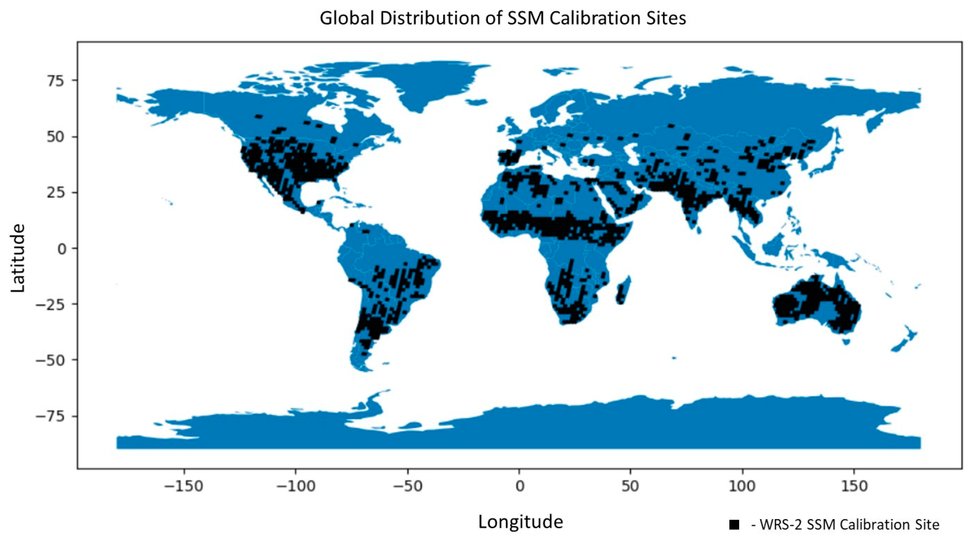
A key component to the success of modeling the mirror’s behavior is an adequate distribution of geometric calibration sites, this is important throughout the event’s image acquisition period but is especially critical during the first few days of an event. As the time and WRS-2 path to start the switch to mode-0 is not a set path, there is a need to have a globally dense set of calibration sites such that the initial, more variable portion of the model, can be modeled adequately for any given time and location that is chosen for the switch from mode-4 to mode-0. Farther in time within an event, a dense set of scenes is not critical as the model becomes more stable and reaches a nearly steady-state. Further complicating this need for a dense set of scenes at the beginning of an event for calibration is the need for a set of cloud-free data throughout the image so as to cover all three SCAs during the OLI-TIRS measurements and calibration step. One catchall to this need for a dense set of calibration sites at the beginning of an event is less desirable sites at times chosen, producing more variability in the measurements than there would be ideally. This, in turn, produces a need for more calibration sites to be used later within an event to reduce the variability within each measurement so as to reach a mean offset from the data measured and the desired estimated encoder position. A combination of using the OLI-to-TIRS alignment geometric calibration sites along with extensive testing during the first several months of the start of the mode-0 operations allowed for a dense set of Worldwide reference (WRS)-2 path/rows that were found to be effective for use in SSM geometric calibration. Note that the OLI-to-TIRS alignment calibration sites are not needed to be as dense as those used for SSM calibration. The changes within with the OLI-to-TIRS alignment, shown in Section 3.2.1, is a much slower varying effect as opposed to the more dynamic SSM mirror behavior early in the event. This allows a more carefully chosen set of sites to be used for the OLI-to-TIRS sensor-to-sensor characterization and calibration where a given measurement is only needed 1–2 times a week. A graph of the WRS-2 path/rows that were used during the mode-0 operations is shown in Figure 4. The plot in Figure 4 represent sites that were chosen on multiple occasions and that typically contained minimal cloud cover. This dense set of geometric calibration sites helps reduce the rare and undesirable choice of scenes with poor correlation characteristics and cloud cover to fill a given void in time (most likely a given path right after a switch to mode-0 operations) where the number of scenes is limited. As was shown previously and will be further demonstrated later, the greatest transition, and hence the greatest movement of the mirror, occurs at the start of the switch to mode-0 and lasts for only a few days, after which the behavior of the mirror starts to stabilize with little to no movement.
Landsat data products are produced in real-time using the best available SSM model at the time of product generation. After the closeout of a given TIRS SSM event, the SSM model is updated a final time, and the products are reprocessed using the final model. These regenerated products can be declared as Tier-1 or Tier-2 depending on the ability to register the scene and if the products meet the 12-m (Tier-1) post-registration accuracy requirements or are above the 12m threshold (Tier-2). In order to have the most accurate mirror calibration with the real-time products, the geometric calibration sites not only need to be well distributed geographically but also need to be used in the calibration in a timely manner. The mirror model is only declared as a final model once the event has closed out and all cloud-free geometric calibration sites can be used within the fitting process. Throughout the event the model is continually updated with the geometric calibration sites, thus continuously refined estimated models are used in real-time product generation. Having a set of calibration scenes available right after the switch to mode-0 with less than 1% cloud cover is critical for having an accurate SSM geometric calibration. Maintaining an adequate set of scenes once the mirror’s behavior becomes more stable and the linear behavior of the mirror is then much easier to obtain.
3. Results and Discussion
Many of the procedures in the processing flow for the end-to-end SSM Geometric Calibration have been automated to increase the quality of the real-time data provided to the user community. The automation minimizes the manual work required to order scenes and process the imagery through the appropriate algorithm steps, and it provides the user community with the higher quality real-time data. These steps help eliminate the analysts need to manually select cloud-free geometric calibration sites, typically with cloud scores of less than 1%, manually having to enter critical items such as the starting time of a beginning of a event, initializing a starting model, or updating the model upon the arrival of the mode-4 encoder data that accompanies the acquisition of the imagery for the first 1–2 orbits upon the switch to mode-0. The last of these benefits the user community by replacing an estimated initial model that must be in place in order to process any imagery with a new model determined from the mode-4 encoder data that are acquired for the short period upon the switch to mode-0 as soon as encoder data becomes available. Some of these automation steps include:
- Event time frames are stored within the IAS database and are entered based on information delivered from the L8 flight operations team (FOT), triggered by email communication from the FOT containing information on the date and time of an upcoming event.
- The initial SSM model needed for generating products at the start of each event is autonomous and triggered by the entry of a given event within the database.
- The ordering of cloud-free scenes over the geometric calibration sites and processing that data through the SSM geometric calibration algorithm is performed periodically throughout the day with a cron job that monitors the product generation status of new imagery arriving in the archive.
- The encoder estimates from the SSM geometric calibration algorithm output are automatically stored in the IAS database based on a given set of threshold criteria pertaining to the registration of both the product and the OLI and TIRS bands.
- The first update of the SSM model based upon the availability of real SSM encoder data is triggered by the first set of encoder data acquired after the start of the event being stored within the IAS database.
One key manual step is the updating of the model based on the SSM geometric calibration results stored in the IAS. The SSM model creation is a user enacted step. The final updating of an SSM model involves a manual and visual inspection of the fitted results from which, upon verification, a new model can be loaded into the IAS database, and a new SSM lookup table can be created for product generation. The last of the steps listed above, the process of updating the initial model based on the first few orbits of real encoder telemetry, allows for a near real-time update to the SSM model to occur within a given event based on the limited mode-4 encoder data that occurs in the first 1–2 orbits upon the switch to mode-0, thus creating better TIRS-to-OLI alignment within hours from the start of the event. This near real time updating of the model is key to providing the best real-time TIRS data possible; this is especially true as it involves the updating of the model based on the real SSM encoder telemetry that occurs after the switch to mode-0 as this is the time period for which the SSM’s behavior is changing the most rapidly.
3.1. SSM Model Fitting
3.1.1. SSM Model
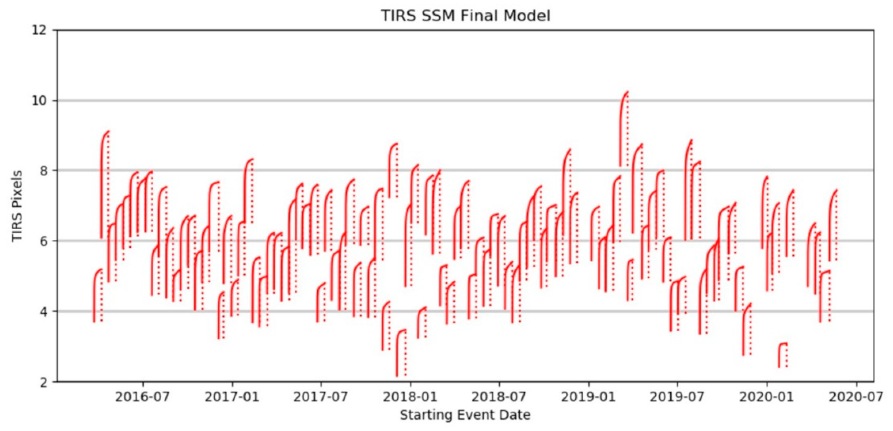
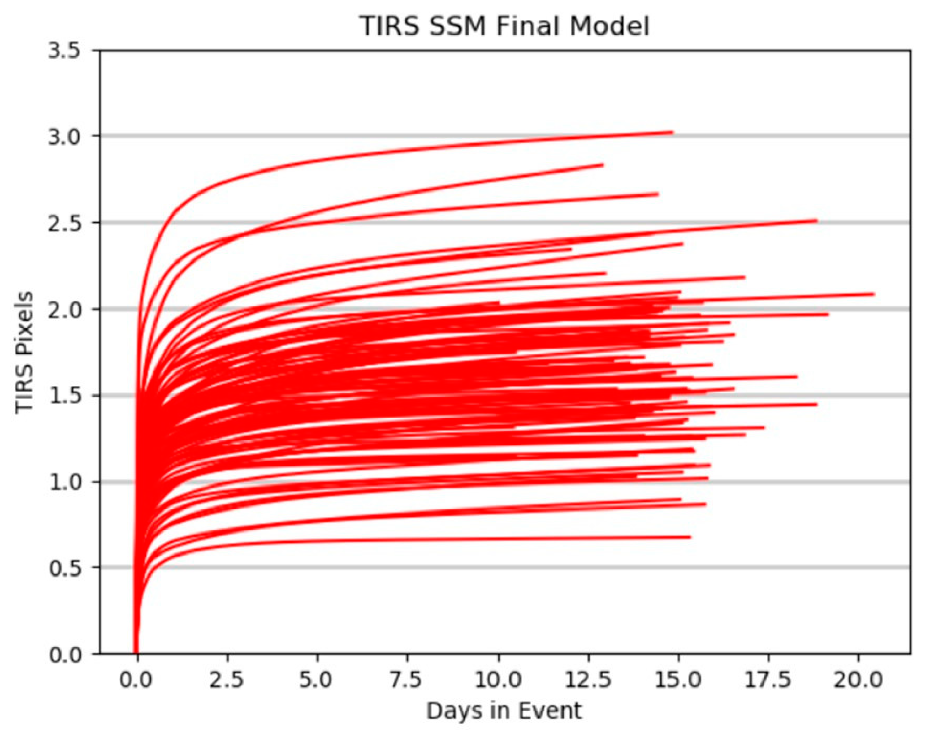
As stated previously, the SSM model’s behavior exhibits its most dynamic behavior at the start of an event, right after the switch to the open-loop mode, then stabilizes within days after this switch. Figure 5 shows the final SSM encoder model for all the SSM events up to early 2020. A dotted line is provided at the end of each event’s function to better identify breaks between events. The figure’s y-axis does not show the actual encoder values for each model but is adjusted for a nominal encoder value so that the y-axis can better demonstrate the differences in the TIRS field of view between models. The x-axis represents the time at which the model is valid, the starting and ending time for a given event, as well as indicating the active model used for product generation. Figure 6 shows the same SSM encoder models from Figure 5; only their starting location is adjusted to start at zero for all models, making the x-axis represent time within an event for each model. Items worth noting from these figures are that the models have essentially the same consistent shape across all events. The starting encoder value for the models can vary by up to 6 TIRS pixels. The location, in days within the event, at which the model starts to level off to a near single steady-state value varies between models, with the final steady-state value itself varying by approximately 2.5 TIRS pixels. The length of each SSM model plotted reflects the time frame for each event (i.e., the time between radiometric calibrations), which varies between events and can differ by several days.
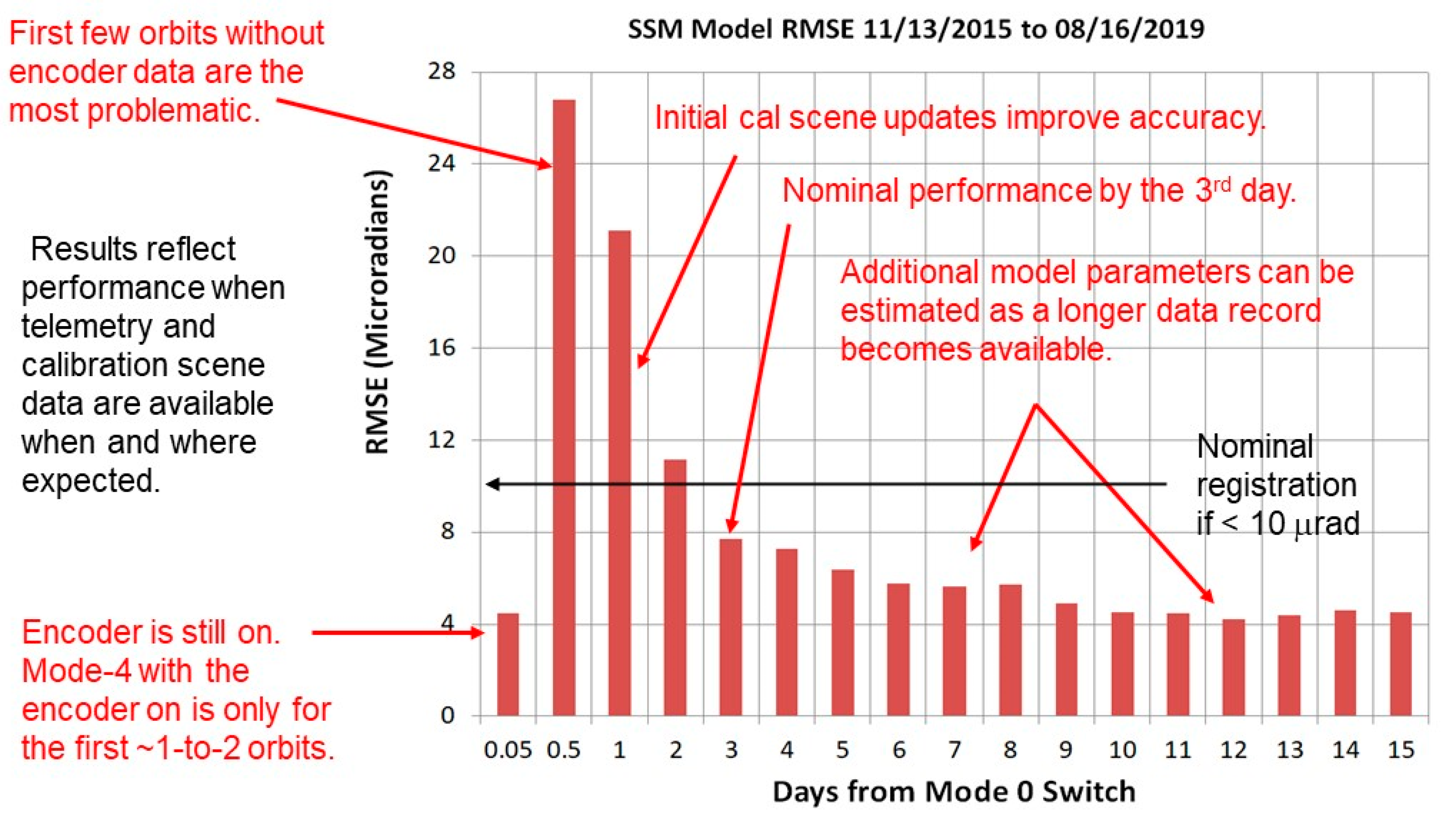
Figure 7 shows the expected error for the SSM calibration broken up by time from the start of the event for the real-time data and products. This figure shows the measured root-mean-square error (RMSE) of the TIRS SSM geometric calibration algorithm for all the scenes used in calibration since the start of the mode-0 operations to early 2020, sorted by the time since the start of the event. The values are plotted to represent the mean error between the measured offset between OLI and TIRS with respect to the mirror’s position used for producing products and the actual value measured within the product across all events. The 0.05 day from the start of an event demonstrates that the first 1 to 1.5 orbits for which the encoder is left on after the start of an event, but the mirror is put within open-loop control and allowed to drift, has the smaller residual error as the encoder represents the best estimate of the mirror’s position. The 0.5 day represents the time period just after the encoder is turned off, and the mirror is still within its most dynamic part of the open-loop control and drifting the most. Therefore, leaving the encoder on at the beginning of each new event, the 0.05 day, is critical to getting an accurate estimate of the mirror behavior both right after the switch to mode-0 and moving forward during its more dramatic behavior with respect to drifting. From the 0.5 day until the closeout of the event of 15+ days, the RMSE measured from the TIRS SSM geometric calibration algorithm continues to fall, reaching a near steady state, with a variability of the only 4 µrad from around 3 days after the start to the end of the event.
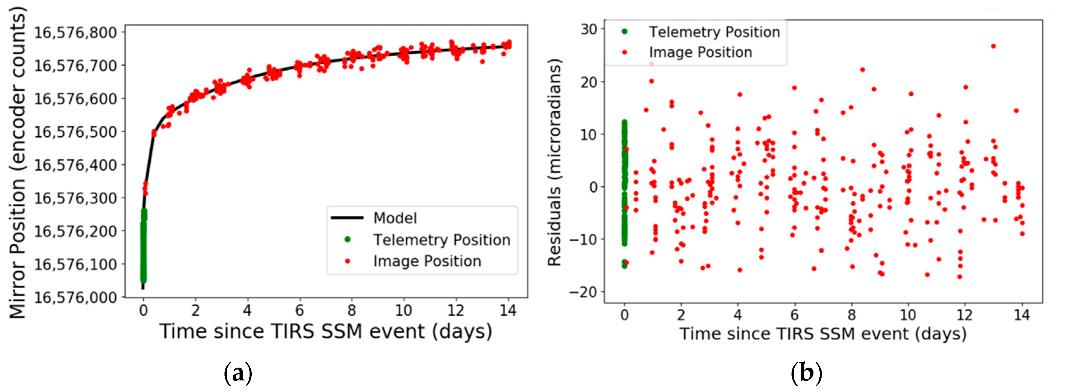
An example of modeling and fitting of the encoder telemetry acquired for the first 1–2 orbits at the start of an event, and all the calibration site measurements within a given event are shown in Figure 8. Figure 8a represents the fitting of the encoder telemetry and calibration site measurements to the SSM model. Figure 8b represents the residuals of the model fit, encoder telemetry, and calibration site measurements shown in Figure 8a. The units for the y-axis in Figure 8a are counts from the 24-bit encoder, representing discrete values defining the 0 to 360° range of the encoder. The y-axis in Figure 8b is microradians. For Figure 8a,b, the x-axis is the number of days from the start of an event. The figure shows the encoder telemetry and how it is acquired only at the very beginning of an event, along with the variability between the calibration site measurements and the model fit.
3.1.2. SSM Model Geometric Calibration Sites
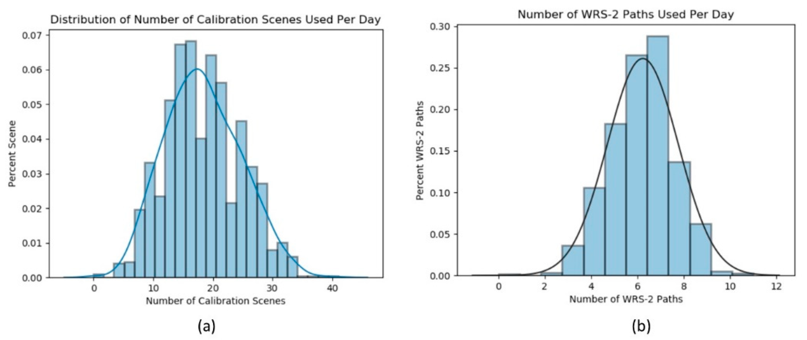
As discussed earlier in this paper, a key component to the successful geometric calibration of the SSM is the ability to obtain image acquisitions over geometric calibration sites where the TIRS to OLI alignment can be measured. Looking over the SSM geometric calibration from the date range of late 2017 to early 2020 gives a view of the use of these geometric calibration sites over time. Figure 9 shows two plots, the plot on the left (9a) gives an indication of the number of scenes used per day, while the plot on the right (9b) shows the number of WRS-2 paths that are used per day. The maximum number of WRS-2 paths that can be used within one day is 15. Figure 9b demonstrates that taking into account that not all WRS-2 paths within a day will have adequate land coverage within a pass in order to be used for calibration, there is an adequate number of paths that are getting used each day for calibration. The plots in Figure 9 show this by representing scene usage in distribution plots calculated by determining the number of geometric calibration sites used per day. Figure 9a supports that for each WRS-2 path that gets used for calibration within a day, there is a dense set of scenes used within at least a subset of all the WRS-2 paths used in calibration. Figure 9a shows that, on average, more than 20 scenes are used to calibrate the SSM mirror per day. Figure 9b shows that for most of the days, scenes from at least six different passes are used in the calibration. Noted previously, the maximum number of Landsat paths possible within a day is 15 and is based on the repeat cycle of the satellite and WRS-2 characteristics. Thus, the calibration scene distribution from these plots shows the diversity of the geometric calibration sites both in the WRS-2 path as well as in the WRS-2 row directions.
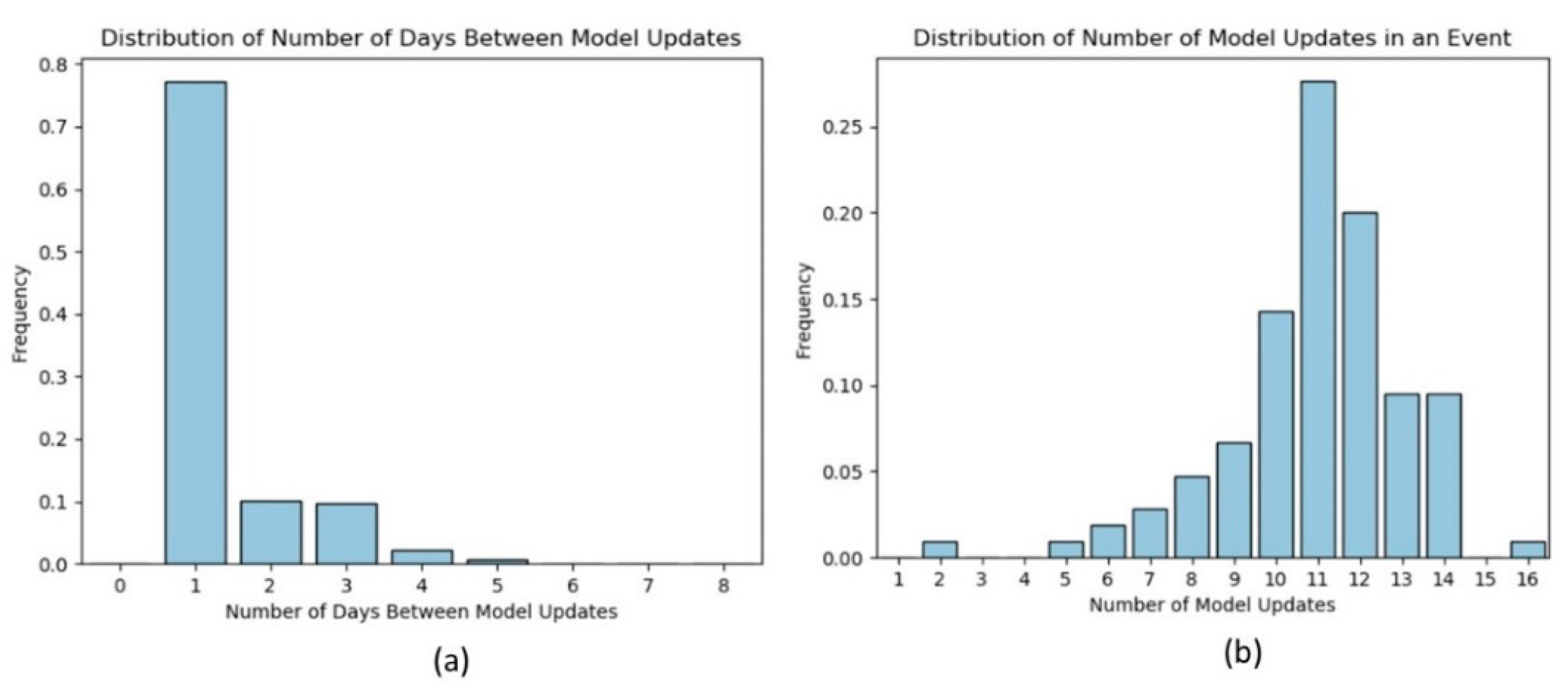
Figure 10 demonstrates the number of measurements used throughout an event; Figure 10 demonstrates the frequency at which the model is updated based on these measurements. From Figure 10a, it is evident that about 77% of the time, SSM geometric calibrations are performed, and the model updates are issued every day. However, at times, the models were updated once in 2 or more days. This occurs predominately during the period for which the model has reached its steady-state response as analysis of these results indicated that the models were updated less frequently during the last few days of the event when all the parameters were well estimated, and the changes in the model coefficients were small due to the “steady-state” nature of the mirror. From Figure 10b, about 80 percent of the events had 10 or more model updates performed during its duration. Note that there were a few events shorter and longer than the nominal 15-day event duration. Typically, the shorter events were associated with an SSM mirror anomaly or other anomaly investigations, and longer time periods were correlated with scheduling conflicts or similar circumstances.
3.2. TIRS Geometric Calibration and Characterization
3.2.1. TIRS Alignment Calibration
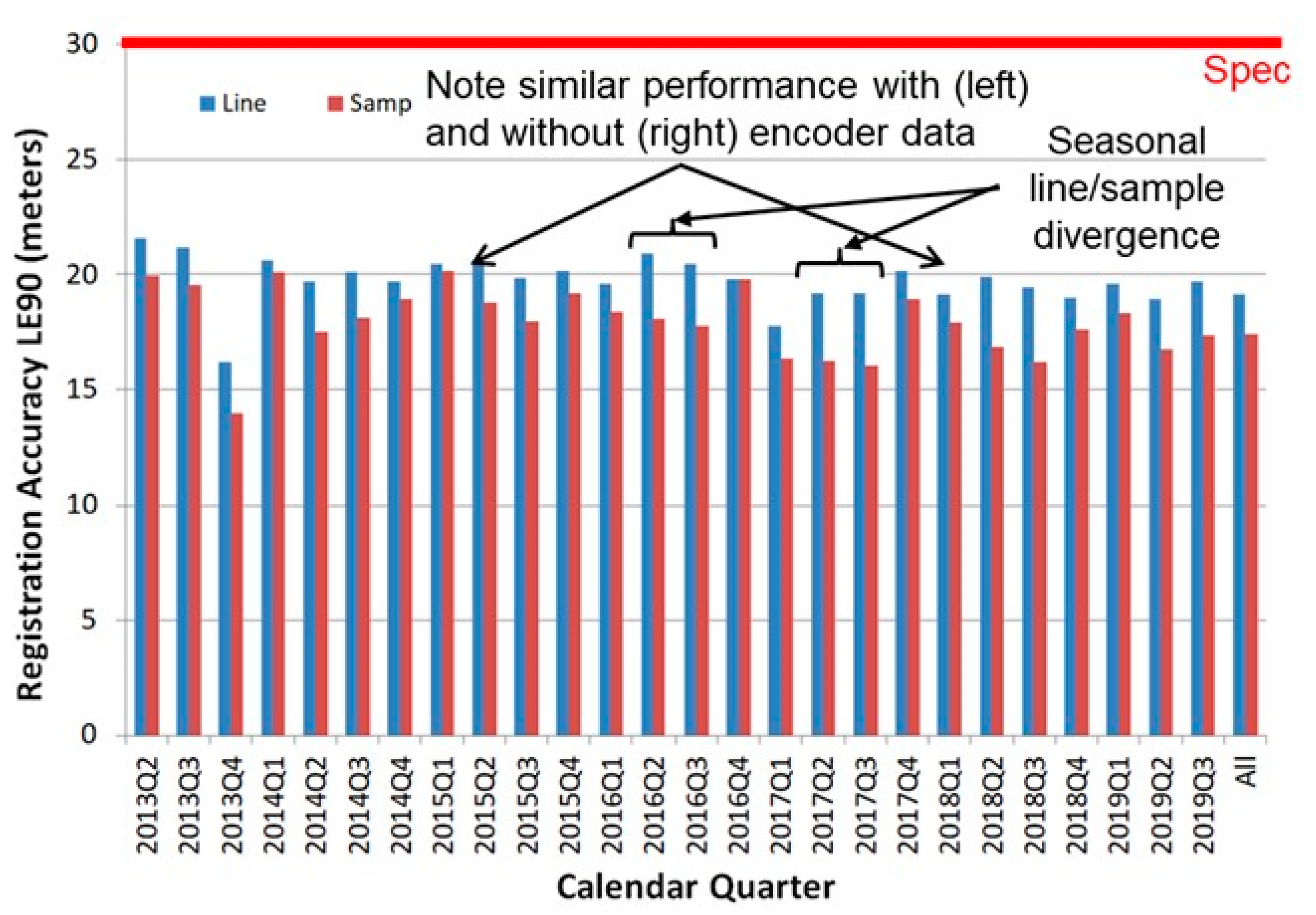
Previously it was shown in Figure 7 the SSM mirror modelling with respect to real time calibration results and demonstrated the ability to improve upon these results as more TIRS SSM Geometric Calibration estimates are included with in the SSM’s modeling. The final outcome to this calibration is the end results, after the preprocessing of the TIRS imagery based on the final SSM mirror model and is the measured TIRS to OLI alignment upon the end of an event and the final SSM model was calculated. These results are shown in Figure 11. Several important notes are highlighted in the graph itself. Upon closure of an event, the mode-4 data acquired prior to the need of any mode-0 set of operations, and the data acquired once the mode-0 set of operations were implemented, the TIRS-to-OLI alignment are equivalent. This is shown by the consistent, less than 10-m variation in the alignment between sensors across the mission’s lifetime. Noted in the graph are seasonal dependencies within the registration results. Starting in 2016, the USGS adopted a data processing collection management structure for its Landsat data products that ensures a consistent set of processing for the Landsat archive within a given collection while allowing a set of calibration updates to be performed between any two given collections. The time frame between 2016 and the end of 2020 was part of the Landsat data collection 1, at the end of 2020 was the start of the Landsat collection 2 data products when these seasonal dependencies are accounted for in processing, these dependencies were not in collection-1 processing. The cause of these seasonal dependencies could be part of the operational procedures of the instrument itself, directly impacting the temperature and the thermal behavior of the optics or mechanics of the mirror; however, these dependencies have not been found to be linked or associated with any spacecraft or instrument telemetry. For collection-2 product generation, these dependencies are accounted for through processing parameters within the Landsat product generation system by setting the TIRS alignment orientation parameters to have values that follow the seasonal differences highlighted in Figure 11.
3.2.2. TIRS Band to Band Characterization
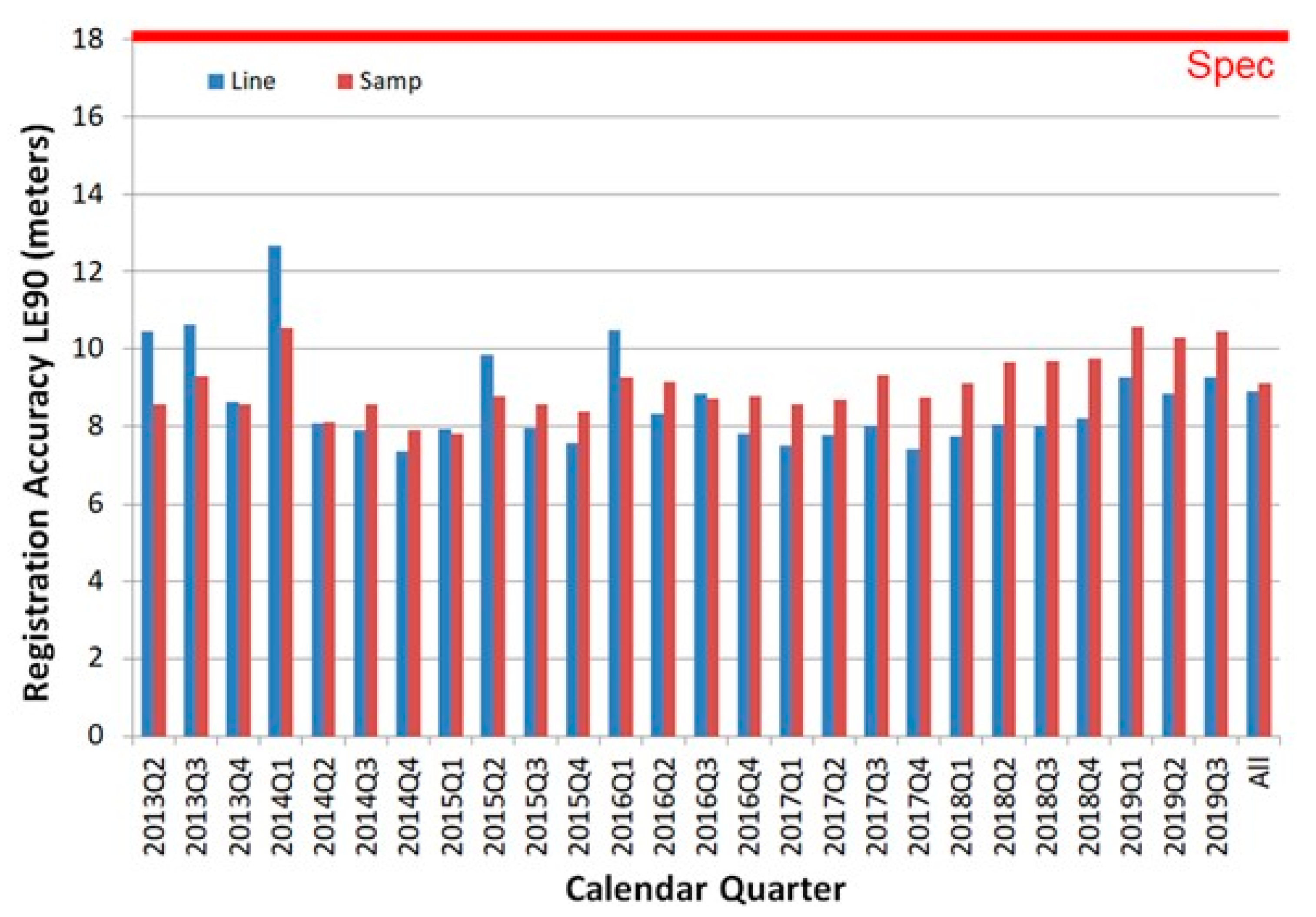
Although not part of the TIRS SSM geometric calibration, band alignment between the two TIRS bands is also characterized as ensuring within instrument registration [8,9]. This characterization is performed after the final TIRS SSM geometric calibration and ensures that both TIRS bands are well registered to the OLI instrument. The Landsat calibration Team ensures that both instruments onboard Landsat 8 are well-calibrated internally and cross-calibrated between each other. The TIRS SSM geometric calibration is only one step in the process. Figure 12 shows the band-to-band registration accuracy of the TIRS instrument from the start of the mission. As can be seen from the graph, the band registration for the TIRS instrument was well within its requirement throughout the mission, regardless of the SSM mode of operations.
4. Conclusions
In this paper the TIRS SSM geometric calibration was discussed with respect to its ground processing operations. In late 2015, both the primary and redundant encoder electronics for the SSM started exhibiting anomalous behavior with respect to anomalous current levels; these events brought about the need to develop a method of operations that limited the use of the SSM encoder electronics, which involved both closed-loop and open-loop control of the mirror. An overview of the processes and steps involved were presented with respect to this mode of operations for the mirror in order to give the perspective of what transpires throughout a TIRS SSM event, defined as the time between radiometric calibration collects, as well as its impact on real-time data. The flexibility in the mirrors pointing model and the ability to establish and use ground calibration sites throughout the globe and have those sites be well distributed in time throughout an SSM event allow for better real-time data to be distributed to the user community. Automation used within the ground processing system to minimize manual involvement also enables the ability for real-time geometric calibration while also reducing the impact for the need of manual calibration throughout the SSM event time frame. On average, it was shown that 20 geometric calibration sites are used within a day for modeling of the mirror, with those 20 scenes coming from a mean of around 6 different WRS-2 paths. All of these aspects of geometric calibration of the SSM are needed due to the variability and unpredictability of the mirror’s behavior when it is placed within its open-loop mode, after the calibration collections needed for establishing radiometric stability for the TIRS instrument. Final SSM geometric calibration results (after reprocessing) were shown, demonstrating that TIRS continues to meet its OLI-to-TIRS alignment requirements by maintaining performance after the switch from the instrument designed mode-4 encoder closed-loop control set of operations to the current mode-0 open-loop set of operations. Finally, it was also shown within this paper that, by frequently updating the model, especially soon after the start of the event, the TIRS-to-OLI alignment could be reduced to around 4 µrad (TIRS Instantaneous Field of View is 1.4186 × 10⁻⁴ rad) within days after the start of the event. Once an SSM event has closed out and a final SSM model has been determined, all the TIRS imagery is reprocessed with this new model, and the TIRS mode-0 imagery will be as well-calibrated as the TIRS imagery that had been previously acquired in mode-4.
Author Contributions
Writing—oringinal darft: M.J.C. and R.R.; Supervision: J.C.S.; Data curation: T.B. All authors have read and agreed to the published version of the manuscript.
Funding
Work performed under USGS contract G15PC00012.
Data Availability Statement
Not applicable.
Conflicts of Interest
The authors declare no conflict of interest.
References
- Irons, J.R.; Dwyer, J.L.; Barsi, J.A. The next Landsat satellite: The Landsat Data Continuity Mission. Remote. Sens. Environ. 2012, 122, 11–21. [Google Scholar] [CrossRef] [Green Version]
- NASA. Landsat Data Continuity Mission Observatory Interface Requirements Document—Revision D6, Document Number GSFC 427-02-03; NASA Goddard Space Flight Center Code 427: Greenbelt, MD, USA, 2009.
- USGS. Landsat 8 (L8) Data Users Handbook; Department of the Interior, U.S. Geological Survey, EROS: Sioux Falls, SD, USA, 2018. Available online: https://www.usgs.gov/core-science-systems/nli/landsat/landsat-8-data-users-handbook (accessed on 26 January 2021).
- Knight, E.J.; Kvaran, G. Landsat-8 Operational Land Imager Design, Characterization and Performance. Remote. Sens. 2014, 6, 10286–10305. [Google Scholar] [CrossRef] [Green Version]
- Reuter, D.C.; Richardson, C.M.; Pellerano, F.A.; Irons, J.R.; Allen, R.G.; Anderson, M.C.; Jhabvala, M.D.; Lunsford, A.; Montanaro, M.; Smith, R.L.; et al. The Thermal Infrared Sensor (TIRS) on Landsat 8: Design Overview and Pre-Launch Characterization. Remote. Sens. 2015, 7, 1135–1153. [Google Scholar] [CrossRef] [Green Version]
- Barsi, J.A.; Markham, B.L.; Montanaro, M.; Hook, S.; Raqueño, N.; Miller, J.A.; Willette, R. Landsat-8 TIRS radiometric calibration status. In Proceedings of the Earth Observing Systems XXV (SPIE), Online, 24 August–4 September 2020; Volume 11501, p. 115010L. [Google Scholar]
- USGS. LDCM Cal/Val Algorithm Description Document—Version 3.0, Document Number LDCM-ADEF-001; U. S. Geological Survey: Sioux Falls, SD, USA, 2013. Available online: https://www.usgs.gov/media/files/landsat-8-9-calibration-validation-algorithm-description-document (accessed on 26 January 2021).
- Storey, J.; Choate, M.J.; Moe, D. Landsat 8 Thermal Infrared Sensor Geometric Characterization and Calibration. Remote. Sens. 2014, 6, 11153–11181. [Google Scholar] [CrossRef] [Green Version]
- Storey, J.; Choate, M.J.; Lee, K. Landsat 8 Operational Land Imager On-Orbit Geometric Calibration and Performance. Remote. Sens. 2014, 6, 11127–11152. [Google Scholar] [CrossRef] [Green Version]
Figure 1.
Red, green, blue (RGB) image containing thermal infrared sensor (TIRS) band 10 for the red channel, operational land imager (OLI) band 7 for the green channel, and OLI band 2 for the blue channel. RGB image demonstrates the overlap between the TIRS and OLI instruments showing that the TIRS instrument field of view is contained within the OLI instrument field of view.

Figure 2.
TIRS instrument showing the scene select mirror which points the TIRS focal plane toward deep space, the blackbody, and Earth collects.
Figure 2.
TIRS instrument showing the scene select mirror which points the TIRS focal plane toward deep space, the blackbody, and Earth collects.

Figure 3.
Processing flow for TIRS scene select mechanism (SSM) geometric calibration. Geometric calibration sites, precision and terrain, and corrected images are used to measure OLI-to-TIRS misalignments that feed the SSM modeling steps. When an adequate number of cloud-free calibration sites are acquired and an SSM model can be determined, new TIRS-to-OLI alignment parameters can be pushed to the Landsat product generation system (LPGS) for product generation. LUT is a lookup table of encoder values used in product generation. LSQ is the non-linear least squares fitting performed on the encoder and image measurements. GUI is the graphical user interface used by the calibration analyst for viewing the SSM encoder function against the encoder and image measurements. ΔP refers to the residual pitch alignment determined from the SSM calibration.

Figure 4.
SSM geometric calibration sites are displayed. Sites are well distributed throughout the globe.
Figure 4.
SSM geometric calibration sites are displayed. Sites are well distributed throughout the globe.

Figure 5.
Position of the SSM with respect to its nominal nadir pointing position. SSM models shown are for each event from 1 March 2016 to 11 May 2020. Variability in the starting angular location is evident from the figure. The dotted lines shown represent the end of the event and not any behavior associated with the mirror itself.

Figure 6.
SSM models from 1 March 2016 to 11 May 2020plotted relative to a start time and date of zero. The length of each plot shows the variability in the length of each event. Variability in the shape of each model is evident, as is the flattening out of the profile as the mirror’s behavior stabilizes farther from the start of the event.

Figure 7.
Bar graph shows the predicted accuracy of the TIRS-to-OLI alignment by the number of days from the start of an event. Accuracy is poorest at the beginning of the event when the mirror movement is the greatest and stabilizes the farther within an event the model transpires.
Figure 7.
Bar graph shows the predicted accuracy of the TIRS-to-OLI alignment by the number of days from the start of an event. Accuracy is poorest at the beginning of the event when the mirror movement is the greatest and stabilizes the farther within an event the model transpires.

Figure 8.
(a) The SSM mirror model for an event along with the encoder telemetry and calibration site measurements used in that model fit. The y-axis is in units of encoder counts; the x-axis is days from the start of the event. (b) The residuals of the fit from the model displayed in (a) with respect to the encoder telemetry and calibration site measurements used in the fit. The y-axis is in units of microradians; the x-axis is days from the start of the event. Encoder telemetry is shown as green dots, while the calibration site measurements are shown as red dots.

Figure 9.
(a) The number of geometric calibration scenes used per day. (b) The number of WRS-2 paths for which geometric calibration scenes are used per day. Both figures demonstrate that the scenes used in the SSM geometric calibration process are well distributed throughout the day.
Figure 9.
(a) The number of geometric calibration scenes used per day. (b) The number of WRS-2 paths for which geometric calibration scenes are used per day. Both figures demonstrate that the scenes used in the SSM geometric calibration process are well distributed throughout the day.

Figure 10.
(a) The number of days between updates to the SSM model. (b) The number of SSM model updates within an event. Both figures represent the frequency for which the model is improved throughout an event.
Figure 10.
(a) The number of days between updates to the SSM model. (b) The number of SSM model updates within an event. Both figures represent the frequency for which the model is improved throughout an event.

Figure 11.
TIRS-to-OLI alignment accuracy is shown broken out by quarters within a calendar year. Seasonal dependencies are pointed to within the figure, as is the demonstration of the accuracy being equivalent once an SSM mode-0 event closes out as compared to the early in mission mode-4 operations of the mirror.

Figure 12.
TIRS instrument, band 10 to band 11, alignment. The within instrument band-to-band alignment of TIRS was below specifications throughout its mission. LE90 is linear error with 90% confidence.
Figure 12.
TIRS instrument, band 10 to band 11, alignment. The within instrument band-to-band alignment of TIRS was below specifications throughout its mission. LE90 is linear error with 90% confidence.

Publisher’s Note: MDPI stays neutral with regard to jurisdictional claims in published maps and institutional affiliations. |
© 2021 by the authors. This work was authored as part of the Contributor’s official duties as an Employee of the United States Government and is therefore a work of the United States Government. In accordance with 17 U.S.C. 105, no copyright protection is available for such works under U.S. Law. This is an Open Access article that has been identified as being free of known restrictions under copyright law, including all related and neighboring rights(https://creativecommons.org/publicdomain/mark/1.0/).You can copy, modify, distribute and perform the work, even for commercial purposes, all without asking permission.
Share and Cite
MDPI and ACS Style
Choate, M.J.; Rengarajan, R.; Storey, J.C.; Beckmann, T. Landsat 8 Thermal Infrared Sensor Scene Select Mechanism Open Loop Operations. Remote Sens. 2021, 13, 617. https://0-doi-org.brum.beds.ac.uk/10.3390/rs13040617
AMA Style
Choate MJ, Rengarajan R, Storey JC, Beckmann T. Landsat 8 Thermal Infrared Sensor Scene Select Mechanism Open Loop Operations. Remote Sensing. 2021; 13(4):617. https://0-doi-org.brum.beds.ac.uk/10.3390/rs13040617
Chicago/Turabian StyleChoate, Michael J., Rajagopalan Rengarajan, James C. Storey, and Tim Beckmann. 2021. "Landsat 8 Thermal Infrared Sensor Scene Select Mechanism Open Loop Operations" Remote Sensing 13, no. 4: 617. https://0-doi-org.brum.beds.ac.uk/10.3390/rs13040617
Note that from the first issue of 2016, this journal uses article numbers instead of page numbers. See further details here.