A Knowledge-Based Auxiliary Channel STAP for Target Detection in Shipborne HFSWR

Abstract

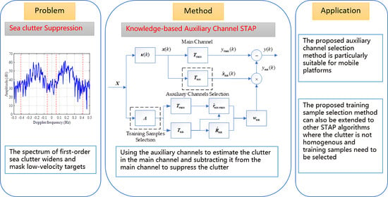
The broadened first-order sea clutter in shipborne high frequency surface wave radar (HFSWR), which will mask the targets with low radial velocity, is a kind of classical space–time coupled clutter. Space–time adaptive processing (STAP) has been proven to be an effective clutter suppression algorithm for space-time coupled clutter. To further improve the efficiency of clutter suppression, a STAP method based on a generalized sidelobe canceller (GSC) structure, named as the auxiliary channel STAP, was introduced into shipborne HFSWR. To obtain precise clutter information for the clutter covariance matrix (CCM) estimation, an approach based on the prior knowledge to auxiliary channel selection is proposed. Auxiliary channels are selected along the clutter ridge of the first-order sea clutter, whose distribution can be determined by the system parameters and regarded as pre-knowledge. To deal with the heterogeneity of the spreading first-order sea clutter, an innovative training samples selection approach according to the Riemannian distance is presented. The range cells that had shorter Riemannian distances to the cell under test (CUT) were chosen as training samples. Experimental results with measured data verified the effectiveness of the proposed algorithm, and the comparison with the existing clutter suppression algorithms showed the superiority of the algorithm.

1. Introduction

In recent years, with the increasing emphasis on marine resources, long-distance detecting, tracking, and early warning of maritime targets have become the top priority of the current maritime rights protection work. High frequency surface wave radar (HFSWR), which achieves over-the-horizon detection of sea-surface targets and sea-skimming targets at low altitude, is an efficient way for ocean surveillance. Compared with shore-based HFSWR, shipborne HFSWR has better survivability, flexibility, and maneuverability. However, the movement of the platform causes the spread of the first-order sea clutter, which will obscure targets with low radial velocity like ships. How to detect the targets submerged in the clutter has become the focus of research on signal processing in shipborne HFSWR.

The premise of clutter suppression is that the clutter and the target are distinguishable in a certain dimension. The characteristics of the clutter and target should be studied before designing a clutter suppression approach. The properties of the spread spectrum of first-order sea clutter has been analyzed and a technique for ship target detection by using the sum-and-difference beamformer was proposed [1]. The space–time distribution of the first-order sea clutter for shipborne HFSWR has been demonstrated and the linear relationship between the Doppler frequency and the azimuth cosine of the first-order sea clutter was pointed out [2]. This means that it is theoretically possible to calculate the azimuth angle of the clutter patch for the determined Doppler frequency unit. Based on this, two spatial projection algorithms, orthogonal weighting (OW) [3] and oblique projection (OP) [4], have been proposed. By projecting the target and clutter to a subspace orthogonal to the clutter subspace, the clutter can be eliminated. Compared with the OW algorithm, the OP algorithm makes the projection space parallel to the target subspace to maintain the gain of the target during the projection process. Nevertheless, the calculated clutter direction is only a theoretical value, and errors often occur in the actual situation, resulting in performance degradation. A linear beamformer has been proposed for clutter cancellation with the help of a flat top beam, difference beam, and an auxiliary estimator beam in [5]. These above approaches suppress clutter by forming nulls in the spatial domain. The difference in azimuth between the target and the clutter is used to separate them.

Considering the difference in the space–time distribution between the first-order sea clutter and the target, suppressing the clutter in the spatial and temporal dimension simultaneously will have better performance. Space–time adaptive processing (STAP) has been proven to be an effective clutter suppression algorithm for this kind of clutter. Some direct-from STAP methods like joint domain localized (JDL), improved orthogonal weighting (IOW), and improved oblique projection (IOP) have been proposed for clutter suppression in shipborne HFSWR [6,7,8,9,10,11,12]. Except for the direct-form processor structure, like the methods above-mentioned, the STAP algorithm can be implemented in the generalized sidelobe canceler (GSC) structure [13]. The GSC is a beamforming structure that can be used as an implementation of linearly constrained adaptive array processors [14] and is a spatial filtering technology. Some main-lobe cancellation methods have been proposed based on this structure for clutter suppression in HFSWR [15,16,17,18,19,20,21,22,23]. A single notch space filter has been designed for target blocking, meanwhile the virtual sliding subarrays were used to obtain secondary beams, which would increase the degree of freedom (DOF) [18,20,21,23]. A rotating spatial beam was proposed [19,22] that works as a blocking matrix and obtains secondary beams for small-aperture arrays. The auxiliary channel STAP is one of the GSC-structure beam-space post-Doppler STAP methods. Only parts of the angle-Doppler channels are selected as auxiliary channels. Unlike JDL processing, which assumes that the angular-Doppler channels surrounding the main channel are most important, the conventional auxiliary channel STAP selects auxiliary channels along the clutter ridge. There are some papers about the application of this clutter suppression method in airborne radar [24,25,26,27,28,29,30,31,32]; however, there is no literature on the application of this method in shipborne HFSWR.

In this paper, the auxiliary channel STAP method was extended to shipborne HFSWR. Improvements were also been made based on the conventional auxiliary channel STAP method to optimize the performance of clutter suppression, which mainly consists of two aspects: one is the prior knowledge based auxiliary channels selecting approach and the other is the training samples selecting approach. The auxiliary channels are selected according to the space–time distribution of the first-order sea clutter to obtain precise clutter information. The training samples were selected according to the Riemannian distance to deal with the heterogeneous clutter in shipborne HFSWR. The rest of this paper is structured as follows. The signal model of shipborne HFSWR is formulated in Section 2. The proposed auxiliary channel STAP algorithm is demonstrated in Section 3. The proposed method was evaluated with measured data in Section 4; Section 5 gives the discussion; and the conclusions are presented in Section 6.

Notation: Scalar quantities are denoted with lightface letters. Vectors and matrices are denoted by boldface lowercase and uppercase letters, respectively. $\mathbb{C}$ represents the complex field. The conjugation of a complex number is denoted by ${\left[\cdot \right]}^{*}$. The transpose, conjugate transpose, and inverse of a matrix are denoted by the superscripts ${\left[\cdot \right]}^T$, ${\left[\cdot \right]}^H$, and ${\left[\cdot \right]}^{-1},$ respectively. The Kronecker product of two matrixes is represented by $\otimes$. The expectation operator is denoted by $E\left[\cdot \right]$. The rounding operator, which indicates rounding to the nearest integer, is denoted by $int\{\cdot \}$. The absolute value of a scalar or the determinant of a square matrix is denoted by $\left|\cdot \right|$. The 2 norm and Frobenius norm of a matrix are denoted by ${\parallel \cdot \parallel }_2$ and ${\parallel \cdot \parallel }_F$, respectively. The trace of a square matrix is represented by $tr\left(\cdot \right)$.

2. Shipborne High Frequency Surface Wave Radar (HFSWR) Signal Model

Assume that the receiving subsystem of the radar consists of N receiving antennas that form a uniform linear array (ULA). The transmitting subsystem transmits a burst of M pulses during the coherent processing interval (CPI). For each channel and each pulse, the received array data are sampled and preprocessed to obtain range samples. The kth range cell takes the form

$$\mathit{x}\left(k\right)={[{\mathit{x}}_1^T {\mathit{x}}_2^T \dots {\mathit{x}}_M^T]}^T,$$

(1)

where ${\mathit{x}}_m={[x_{1,m} x_{2,m} \dots x_{N,m}]}^T, m=1,2,\dots M$ represents the data collected from the mth pulse and ${\left[\cdot \right]}^T$ denotes transposition.

The received data snapshot $\mathit{x}\left(k\right)\in {\mathbb{C}}^{MN\times 1}$ is the sum of three parts, target, clutter, and noise, denoted $\mathit{s}\left(k\right)$, $\mathit{c}\left(k\right)$, and $\mathit{n}\left(k\right)$, respectively. It is mathematically written as

$$\mathit{x}\left(k\right)=\mathit{s}\left(k\right)+\mathit{c}\left(k\right)+\mathit{n}\left(k\right).$$

(2)

The target snapshot, denoted $\mathit{s}\left(k\right)\in {\mathbb{C}}^{MN\times 1}$, can be expressed as the product of complex amplitude ${\sigma }_{\mathrm{tgt}}$ and space–time steering vector ${\mathit{v}}_{\mathrm{tgt}}$, and can be written as

$$\mathit{s}\left(k\right)={\sigma }_{\mathrm{tgt}}{\mathit{v}}_{\mathrm{tgt}},$$

(3)

where the space–time steering vector of the target, denoted ${\mathit{v}}_{\mathrm{tgt}}\in {\mathbb{C}}^{MN\times 1}$, is the Kronecker product of the spatial steering vector $\mathit{a}\left({\theta }_{\mathrm{tgt}}\right)\in {\mathbb{C}}^{N\times 1}$ and the temporal steering vector $\mathit{b}\left(f_{\mathrm{tgt}}\right)\in {\mathbb{C}}^{M\times 1}$, and is written as

$${\mathit{v}}_{\mathrm{tgt}}=\mathit{b}\left(f_{\mathrm{tgt}}\right)\otimes \mathit{a}\left({\theta }_{\mathrm{tgt}}\right),$$

(4)

where the mathematical symbol $\otimes$ is the Kronecker product. The spatial steering vector and the temporal steering vector take the form,

$$\mathit{a}\left({\theta }_{\mathrm{tgt}}\right)={\left[1 e^{j2\pi \cdot f_s} e^{j2\pi \cdot 2f_s} \dots e^{j2\pi \cdot \left(N-1\right)f_s}\right]}^T,$$

(5)

$$\mathit{b}\left(f_{\mathrm{tgt}}\right)={\left[1 e^{j2\pi \cdot f_t} e^{j2\pi \cdot 2f_t} \dots e^{j2\pi \cdot \left(M-1\right)f_t}\right]}^T,$$

(6)

where $f_s=\left(d/\lambda \right)sin{\theta }_{\mathrm{tgt}}$ and $f_t=f_{\mathrm{tgt}}\cdot t_R$ are the normalized spatial and Doppler frequency, respectively. The symbols $\lambda$ and d represent the wavelength and the interelement spacing of the ULA, respectively. The azimuth of the target and the Doppler frequency of the target are denoted by ${\theta }_{\mathrm{tgt}}$ and $f_{\mathrm{tgt}}$, respectively. The pulse repetition interval (PRI) is denoted by $t_R$.

Thus, the covariance matrix of the target signal can be derived as

$${\mathit{R}}_s=E\left[\mathit{s}\left(k\right){\mathit{s}}^H\left(k\right)\right]={\sigma }_{\mathrm{tgt}}^2{\mathit{v}}_{\mathrm{tgt}}{\mathit{v}}_{\mathrm{tgt}}^H,$$

(7)

where $E\left[\cdot \right]$ indicates the expectation operator.

The clutter snapshot $\mathit{c}\left(k\right)\in {\mathbb{C}}^{MN\times 1}$ in HFSWR is mainly composed of the first-order and second-order sea clutter, and the energy of the second-order sea clutter is usually 20–45 dB smaller than that of the first-order [33]. Therefore, the second-order sea clutter can be ignored. The clutter in a certain range cell can be regarded as the superposition of a large number of uncorrelated clutter patches [34,35], which has the expression as follows,

$$\mathit{c}\left(k\right)={\displaystyle \sum }_{q=1}^{N_c}{\sigma }_{1,q}{\mathit{v}}_{1,q}+{\displaystyle \sum }_{q=1}^{N_c}{\sigma }_{2,q}{\mathit{v}}_{2,q}={\displaystyle \sum }_{q=1}^{N_c}{\sigma }_{1,q}\mathit{b}\left(f_{1,q}\right)\otimes \mathit{a}\left({\theta }_{\mathrm{q}}\right)+{\displaystyle \sum }_{q=1}^{N_c}{\sigma }_{2,q}\mathit{b}\left(f_{2,q}\right)\otimes \mathit{a}\left({\theta }_{\mathrm{q}}\right),$$

(8)

where $q=1,2,\dots ,N_c$ denotes the qth clutter patch in the kth range bin; the complex amplitude of the receding (caused by ocean waves going away from the radar) and approaching (caused by ocean waves coming toward the radar) first-order ocean clutter are denoted by ${\sigma }_{1,q}$ and ${\sigma }_{2,q}$, respectively; their corresponding Doppler frequency are denoted by $f_{1,q}$ and $f_{2,q}$, respectively; and the azimuth of the qth clutter patch in the kth range bin is denoted by ${\theta }_q$. Under ideal conditions, there is a linear relationship between the Doppler frequency $f_{i,q}, i=1,2$ and the azimuth cosine $cos\left({\theta }_q\right)$ of the clutter patch, as described in [2],

$$f_{i,q}=(-1{)}^i{f}_B+\frac{2v_p}{\lambda }cos({\theta }_q), i=1,2,$$

(9)

where $v_p$ denotes the platform velocity. The symbol $f_B\approx 0.102\sqrt{f_0}$ is the first-order Bragg frequency, and is calculated using the system carrier frequency $f_0$ in MHz.

The the clutter covariance matrix (CCM) was analyzed in [34,35] and has the following expression

$$\begin{array}{ll}{\mathit{R}}_c& =E\left[\mathit{c}\left(k\right){\mathit{c}}^H\left(k\right)\right]\\ & ={\displaystyle {\displaystyle \sum }_{q=1}^{N_c}}{\sigma }_{1,q}^2{\mathit{v}}_{1,q}{\mathit{v}}_{1,q}^H+{\displaystyle {\displaystyle \sum }_{q=1}^{N_c}}{\sigma }_{2,q}^2{\mathit{v}}_{2,q}{\mathit{v}}_{2,q}^H+{\displaystyle {\displaystyle \sum }_{q=1}^{N_c}}{\sigma }_{1,q}{\mathit{v}}_{1,q}{\sigma }_{2,q}^{*}{\mathit{v}}_{2,q}^H+{\displaystyle {\displaystyle \sum }_{q=1}^{N_c}}{\sigma }_{2,q}{\mathit{v}}_{2,q}{\sigma }_{1,q}^{*}{\mathit{v}}_{1,q}^H.\end{array}$$

(10)

For a fully-developed sea where the energy supplied by the wind is equal to the energy lost in breaking waves, its surface is a random surface. According to [34,36,37], the random amplitudes of the harmonic components of electromagnetic waves scattered off a random surface are uncorrelated. Thus, the first-order sea clutter from different ocean patches can be assumed as uncorrelated. The complex amplitudes of the preceding and approaching Bragg components from the same clutter patch are also assumed to be uncorrelated. The CCM is simplified to

$$\begin{array}{ll}{\mathit{R}}_c& ={\displaystyle {\displaystyle \sum }_{q=1}^{N_c}}{\sigma }_{1,q}^2{\mathit{v}}_{1,q}{\mathit{v}}_{1,q}^H+{\displaystyle {\displaystyle \sum }_{q=1}^{N_c}}{\sigma }_{2,q}^2{\mathit{v}}_{2,q}{\mathit{v}}_{2,q}^H\\ & ={\mathit{R}}_{1c}+{\mathit{R}}_{2c}.\end{array}$$

(11)

The rank of the CCM for shipborne HFSWR is derived in a precise expression in [35], as

$$\mathrm{rank}\left({\mathit{R}}_c\right)=int\{2\alpha \left[N-1+\beta \left(M-1\right)\right]+2\},$$

(12)

where the factors $\alpha$ and $\beta$ are calculated as $\alpha =\frac{2d}{\lambda }$ and $\beta =\frac{2v_p{t}_R}{d}$; the PRI $t_R$ in $\beta$ is calculated as $t_R=\frac{1}{f_R}$; and the operator $int\{\cdot \}$ indicates rounding to the nearest integer.

The noise snapshot $\mathit{n}\left(k\right)\in {\mathbb{C}}^{MN\times 1}$ can be assumed as a complex Gaussian distribution with zero-mean and the power ${\sigma }_n^2$. The noise covariance matrix is

$${\mathit{R}}_n=E\left[\mathit{n}\left(k\right){\mathit{n}}^H\left(k\right)\right]={\sigma }_n^2{\mathit{I}}_{MN}.$$

(13)

3. Knowledge-Based Auxiliary Channel Space–Time Adaptive Processing (STAP)

Auxiliary channel STAP is one of the GSC-structure STAP methods. The core of auxiliary STAP is to estimate the clutter in the main channel using the clutter in auxiliary channels. In this section, a knowledge-based auxiliary channel STAP algorithm is presented for spreading sea clutter suppression in shipborne HFSWR.

3.1. Auxiliary Channel Space–Time Adaptive Processing (STAP)

For the kth range cell data $\mathit{x}\left(k\right)$, assume that the azimuth of the target and the Doppler frequency of the target are denoted by ${\theta }_{\mathrm{tgt}}$ and $f_{\mathrm{tgt}}$, respectively.

The main channel, denoted by ${\tilde{x}}_{\mathrm{main}}\left(k\right)\in {\mathbb{C}}^{1\times 1}$, is calculated as

$${\tilde{x}}_{\mathrm{main}}\left(k\right)={\mathit{T}}_{\mathrm{main}}^H\mathit{x}\left(k\right),$$

(14)

where ${\mathit{T}}_{\mathrm{main}}\in {\mathbb{C}}^{MN\times 1}$ is the transformation matrix, which has the same representation with the space–time steering vector of the target,

$${\mathit{T}}_{\mathrm{main}}={\mathit{v}}_{tgt}=\mathit{b}\left(f_{\mathrm{tgt}}\right)\otimes \mathit{a}\left({\theta }_{\mathrm{tgt}}\right).$$

(15)

Assume that D auxiliary channels are selected, the auxiliary channels, denoted by ${\tilde{\mathit{x}}}_{\mathrm{aux}}\left(k\right)\in {\mathbb{C}}^{D\times 1}$, are calculated as,

$${\tilde{\mathit{x}}}_{\mathrm{aux}}\left(k\right)={\mathit{T}}_{\mathrm{aux}}^H\mathit{x}\left(k\right),$$

(16)

where ${\mathit{T}}_{\mathrm{aux}}\in {\mathbb{C}}^{MN\times D}$ is the transformation matrix for auxiliary channels.

After transforming into the angle-Doppler domain, the main channel data ${\tilde{x}}_{\mathrm{main}}\left(k\right)$ is the sum of the target, the first-order sea clutter, and noise. As the following equation denotes,

$${\tilde{x}}_{\mathrm{main}}\left(k\right)={\tilde{s}}_{\mathrm{main}}\left(k\right)+{\tilde{c}}_{\mathrm{main}}\left(k\right)+{\tilde{n}}_{\mathrm{main}}\left(k\right).$$

(17)

If the clutter in the auxiliary channels is related to that in the main channel, it can be estimated from the auxiliary channels. This estimation, denoted by $y_{\mathrm{aux}}\left(k\right)\in {\mathbb{C}}^{1\times 1}$, is named as the output of auxiliary channels, and can be denoted by the following equation,

$$y_{\mathrm{aux}}\left(k\right)={\mathit{w}}_{\mathrm{aux}}^H{\tilde{\mathit{x}}}_{\mathrm{aux}}\left(k\right)={\widehat{\tilde{c}}}_{\mathrm{main}}\left(k\right)+{\widehat{\tilde{n}}}_{\mathrm{main}}\left(k\right)\in {\mathbb{C}}^{1\times 1}.$$

(18)

Subtracting the estimated clutter plus noise ${\widehat{\tilde{c}}}_{\mathrm{main}}\left(k\right)+{\widehat{\tilde{n}}}_{\mathrm{main}}\left(k\right)$ from the main channel and the output of the auxiliary channel STAP processor, $y\left(k\right)\in {\mathbb{C}}^{1\times 1}$ is

$$\begin{array}{ll}y\left(k\right)& ={\tilde{x}}_{\mathrm{main}}\left(k\right)-y_{\mathrm{aux}}\left(k\right)\\ & ={\tilde{s}}_{\mathrm{main}}\left(k\right)+{\tilde{c}}_{\mathrm{main}}\left(k\right)+{\tilde{n}}_{\mathrm{main}}\left(k\right)-{\widehat{\tilde{c}}}_{\mathrm{main}}\left(k\right)+{\widehat{\tilde{n}}}_{\mathrm{main}}\left(k\right)\\ & ={\tilde{s}}_{\mathrm{main}}\left(k\right)+\tilde{\epsilon }\left(k\right),\end{array}$$

(19)

where $\tilde{\epsilon }\left(k\right)={\tilde{c}}_{\mathrm{main}}\left(k\right)+{\tilde{n}}_{\mathrm{main}}\left(k\right)-{\widehat{c}}_{\mathrm{main}}\left(k\right)-{\widehat{n}}_{\mathrm{main}}\left(k\right)$ is the residual term of the clutter and noise.

The weights vector ${\mathit{w}}_{\mathrm{aux}}$ can be determined by the solution of the following least squares problem

$$\underset{{\mathit{w}}_{\mathrm{aux}}}{min}\parallel y_{\mathrm{main}}\left(k\right)-y_{\mathrm{aux}}{\left(k\right)\parallel }_2^2=\underset{{\mathit{w}}_{\mathrm{aux}}}{min}\parallel \left[{\mathit{T}}_{\mathrm{main}}^H-{\mathit{w}}_{\mathrm{aux}}^H{\mathit{T}}_{\mathrm{aux}}^H\right]\mathit{x}{\left(k\right)\parallel }_2^2.$$

(20)

The solution is given by

$${\mathit{w}}_{\mathrm{aux}}={\mathit{R}}_{\mathrm{aux}}^{-1}{\mathit{r}}_{\mathrm{aux}-\mathrm{main}}\in {\mathbb{C}}^{D\times 1},$$

(21)

$${\mathit{R}}_{\mathrm{aux}}=E\{{\tilde{\mathit{x}}}_{\mathrm{aux}}\left(k\right){\tilde{\mathit{x}}}_{\mathrm{aux}}^H\left(k\right)\}\in {\mathbb{C}}^{D\times D},$$

(22)

$${\mathit{r}}_{\mathrm{aux}-\mathrm{main}}=E\left\{{\tilde{\mathit{x}}}_{\mathrm{aux}}\left(k\right){\tilde{x}}_{\mathrm{main}}^{*}\left(k\right)\right\}\in {\mathbb{C}}^{D\times 1},$$

(23)

where ${\mathit{R}}_{\mathrm{aux}}$ is the self-correlation matrix of the auxiliary channel, and ${\mathit{r}}_{\mathrm{aux}-\mathrm{main}}$ is the cross-correlation vector between the auxiliary channels and the main channel.

It is worth noting that ${\mathit{R}}_{\mathrm{aux}}$ and ${\mathit{r}}_{\mathrm{aux}-\mathrm{main}}$ are unknown in practice and the maximum likelihood estimate is commonly used

$${\widehat{\mathit{R}}}_{\mathrm{aux}}=\frac{1}{K}{\displaystyle \sum }_{k=1}^K{\tilde{\mathit{x}}}_{\mathrm{aux}}\left(k\right){\tilde{\mathit{x}}}_{\mathrm{aux}}^H\left(k\right),$$

(24)

$${\widehat{\mathit{r}}}_{\mathrm{aux}-\mathrm{main}}=\frac{1}{K}{\displaystyle \sum }_{k=1}^K{\tilde{\mathit{x}}}_{\mathrm{aux}}\left(k\right){\tilde{x}}_{\mathrm{main}}^{*}\left(k\right),$$

(25)

where ${\tilde{\mathit{x}}}_{\mathrm{aux}}\left(k\right), k=1,2,\dots ,K$, ${\tilde{x}}_{\mathrm{main}}\left(k\right), k=1,2,\dots ,K$ are the secondary data.

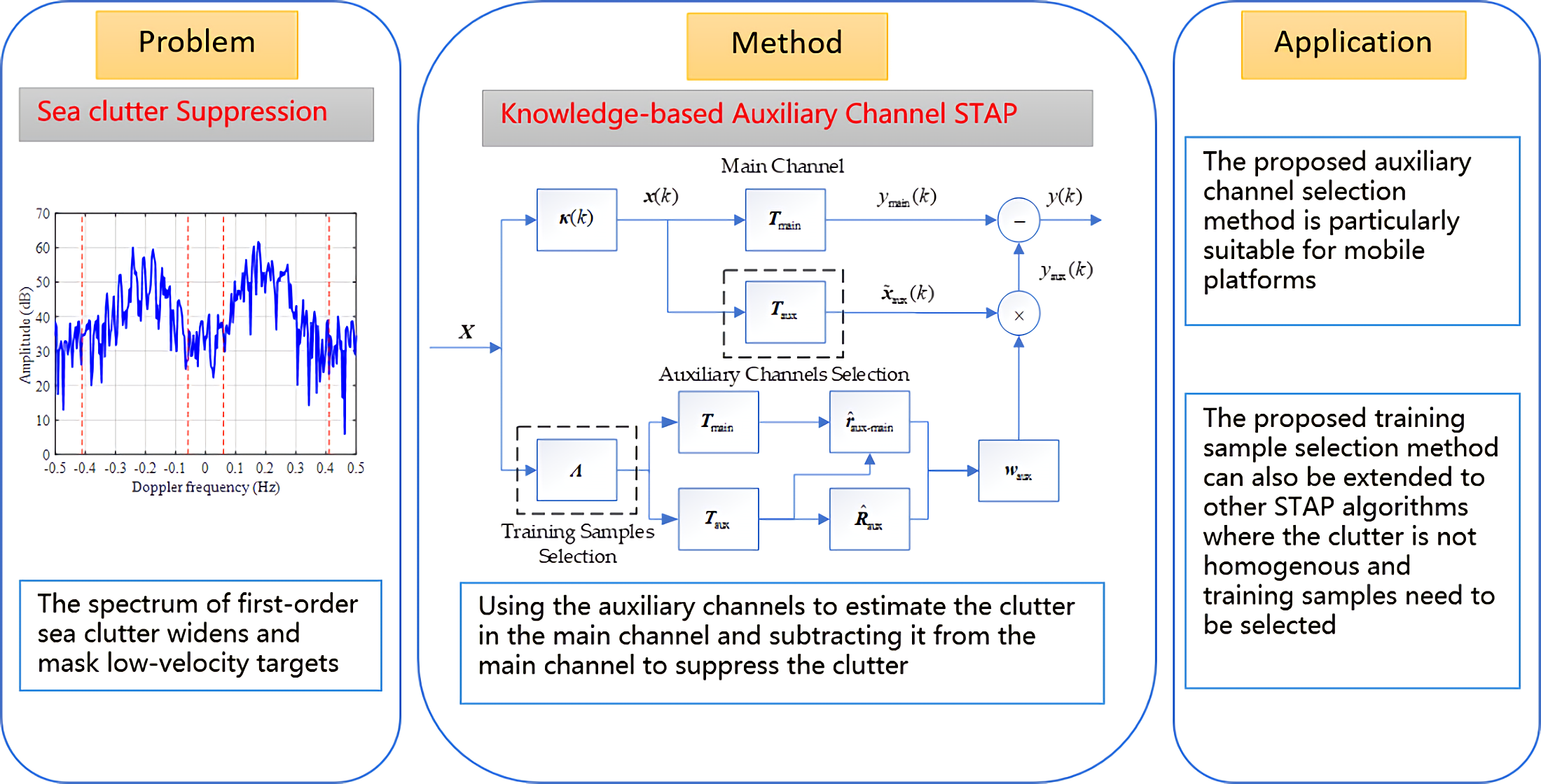
The framework of the auxiliary channel STAP algorithm is illustrated in Figure 1.

As shown in Figure 1, for the input range cell data $\mathit{x}\left(k\right)$, after a transformation (Doppler processing and beam forming), the data are converted into the beam-Doppler space, and the auxiliary channels are selected in it. After that, the adaptive weight vector of the auxiliary channels is calculated according to the minimum mean square error (MMSE) criterion and the output of the auxiliary channels is calculated. Finally, the output of the auxiliary channels is subtracted from the main channel output to suppress the clutter.

The performance of the auxiliary channel STAP method is mainly affected by how the auxiliary channels are selected and the estimation accuracy of the weights vector ${\mathit{w}}_{\mathrm{aux}}$. The selection of auxiliary channels is determined as the transformation matrix ${\mathit{T}}_{\mathrm{aux}}$ and the estimation accuracy of ${\mathit{w}}_{\mathrm{aux}}$ is determined by the training samples used when calculating the self-correlation matrix ${\mathit{R}}_{\mathrm{aux}}$ and cross-correlation vector ${\mathit{r}}_{\mathrm{aux}-\mathrm{main}}$. Therefore, for these two directions, a knowledge-based auxiliary channel selection approach and a training sample selection approach are proposed in Section 3.2 and Section 3.3 to improve the performance of the auxiliary channel STAP method.

3.2. Knowledge-Based Auxiliary Channels Selection

For shipborne HFSWR, the distribution of the first-order sea clutter is two straight lines on the angle-Doppler plane. Setting $f_{i,q}$ as abscissa and $cos({\theta }_q)$ as the vertical coordinate, Equation (9) is rewritten as $x=\pm f_B+\frac{2v_p}{\lambda }y$. After transformation, the formula $y=\frac{\lambda }{2v_p}x\mp \frac{\lambda }{2v_p}{f}_B$ is obtained. The wavelength $\lambda$, the platform velocity $v_p$, and the Bragg frequency $f_B$ are constant. Hence, two single straight lines (clutter ridge) are expected in the angle-Doppler domain. One is the negative part $y=\frac{\lambda }{2v_p}x+\frac{\lambda }{2v_p}{f}_B$, and the other is the positive part $y=\frac{\lambda }{2v_p}x-\frac{\lambda }{2v_p}{f}_B$. These two straight lines are determined by system parameters and can be seen as prior knowledge.

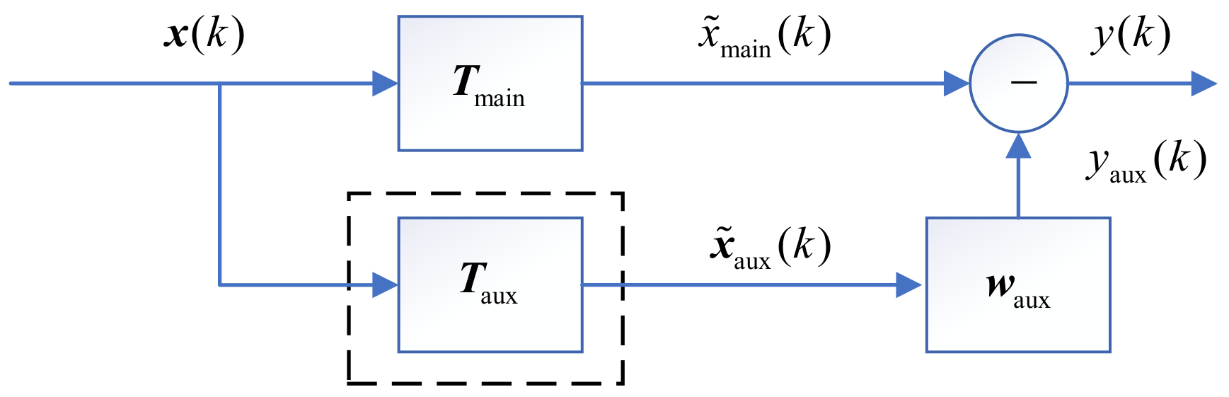
A data acquisition experiment was conducted in the Yellow Sea of China in September 1998. The data acquisition system consists of a transmitting subsystem, a receiving subsystem, and a data acquisition subsystem. The transmitting subsystem is made of an omnidirectional antenna, and the signal used is frequency modulated interrupted continuous wave (FMICW). The receiving subsystem includes seven antennas that form a uniform linear broadside array. The geometry of the receiving array is illustrated in Figure 2.

The whole system was mounted on a barge, which was tugged by a tugboat. As described in [1,3,7,12], the system parameters are shown in

Table 1. System parameters [12].

Parameters	Symbol	Value
platform velocity	$v_p$	5 m/s
number of antennas	$N$	7
distance between antennas	$d$	14 m
frequency	$f_0$	5.283 MHz
bandwidth	$B$	30 KHz
pulse repetition interval	$T$	0.262144 s
sampling frequency	$f_s$	976.5625 Hz

.

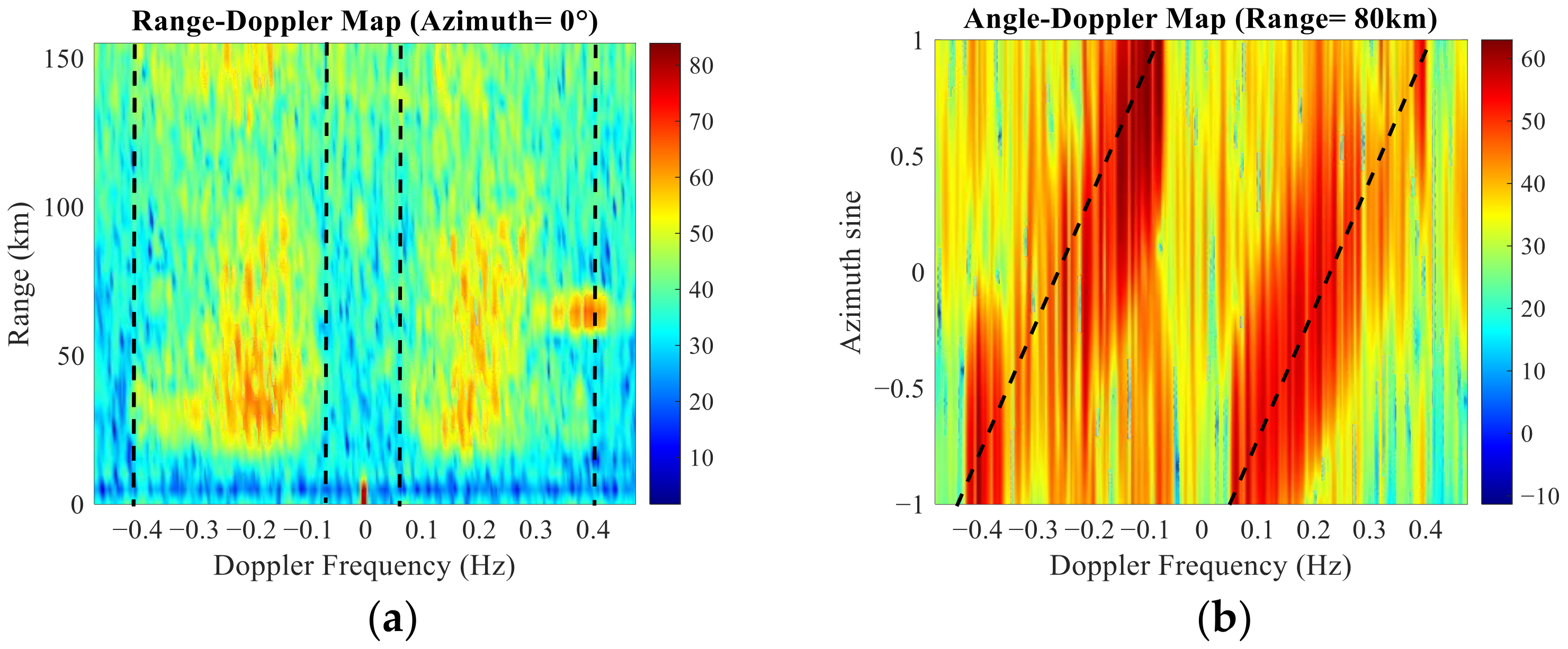
Figure 3 illustrates the range-Doppler map and the angle-Doppler map of the measured data. The dashed line in Figure 3a represents the spreading region of the first-order sea clutter. The dashed line in Figure 3b denotes the clutter ridge.

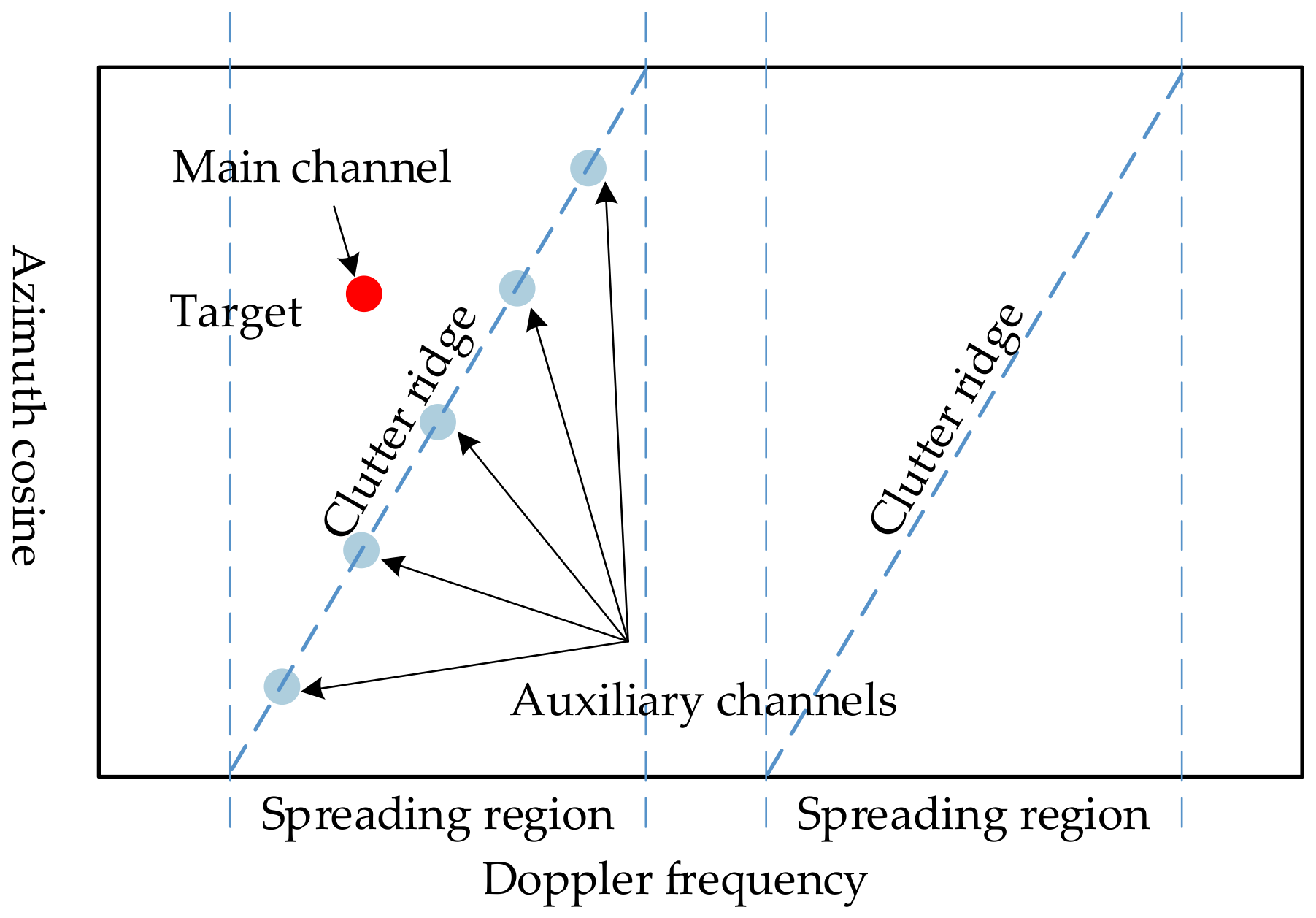
For auxiliary channel STAP, auxiliary channels should contain clutter with the same characteristics as the main channel. Due to the wider beam width in the spatial domain, the main channel will contain some clutter components from the clutter ridge. Thus, we can utilize this prior knowledge and select auxiliary channels along the clutter ridge of the first-order sea clutter. Figure 4 shows the sketch map of the main channel and auxiliary channels. If the targets fall in the spreading range of the first-order sea clutter, the clutter plus noise component ${\tilde{c}}_{\mathrm{main}}\left(k\right)+{\tilde{n}}_{\mathrm{main}}\left(k\right)$ in the main channel can be approximated from the clutter ridge.

According to the prior knowledge, the auxiliary channels selecting matrix ${\mathit{T}}_{\mathrm{aux}}$ were chosen as a set of the space–time steering vectors of the first-order sea clutter.

$${\mathit{T}}_{\mathrm{aux}}=\left[{\mathit{v}}_{c_1} {\mathit{v}}_{c_2} \cdots {\mathit{v}}_{c_D}\right],$$

(26)

$${\mathit{v}}_{c_i}=\mathit{b}\left(f_{c_i}\right)\otimes \mathit{a}\left({\theta }_{c_i}\right),$$

(27)

where $f_{c_i}, i=1,2,\dots ,D$ and ${\theta }_{c_i}, i=1,2,\dots ,D$ are the Doppler frequency and the azimuth of the clutter patches, respectively. They satisfy Equation (9).

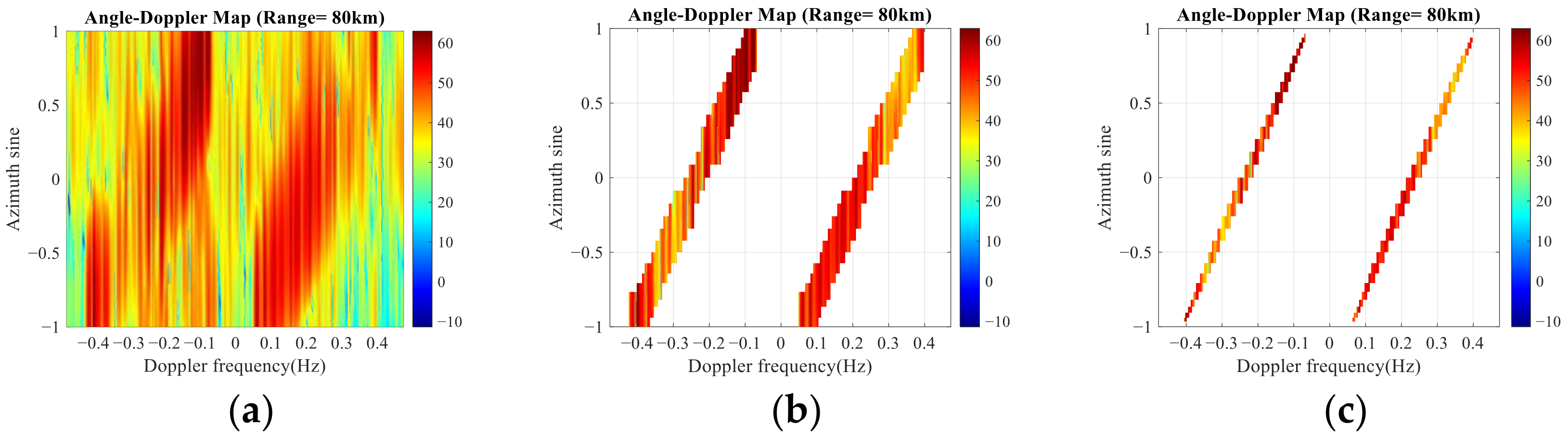
The quantity of auxiliary channels, denoted by D, is discussed as follows. The total number of auxiliary channels available is determined by how the clutter ridge is defined. Figure 5 illustrates the theoretical clutter ridge and two different extracted clutter ridges from the measured data.

Taking the theoretical clutter ridge in Figure 5a as an example, the quantity of auxiliary channels available when only one beam channel is selected for a determined Doppler frequency, can be calculated as

$$D=int\left\{\frac{4v_p}{\lambda d_{res}}\right\},$$

(28)

where $d_{res}$ represents the Doppler resolution. In this situation, the number of auxiliary channels is equal to the number of Doppler channels. According to Equation (9), the spreading range of first-order sea clutter is $\left[-f_B-\frac{2v_p}{\lambda }-f_B+\frac{2v_p}{\lambda }\right]$ in the negative Doppler frequency and $\left[f_B-\frac{2v_p}{\lambda } f_B+\frac{2v_p}{\lambda }\right]$ in the positive Doppler frequency. The number of Doppler channels is $int\left\{\frac{4v_p}{\lambda d_{res}}\right\}$ in the positive part or the negative part. Hence, the quantity of auxiliary channels is $int\left\{\frac{4v_p}{\lambda d_{res}}\right\}$. This usually numbers between tens and hundreds, which means that there are plenty of auxiliary channels for selecting.

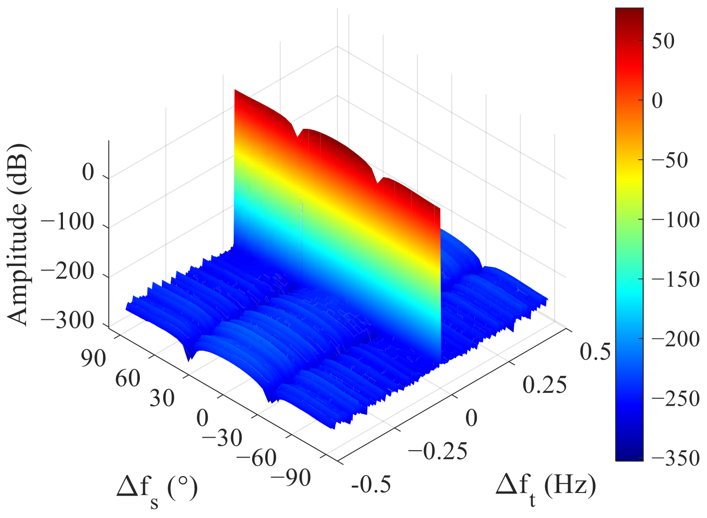
It is worth noting that ${\mathit{T}}_{\mathrm{aux}}$ also works as the blocking matrix and should satisfy ${\mathit{T}}_{\mathrm{aux}}^H{\mathit{T}}_{\mathrm{main}}={\mathit{T}}_{\mathrm{aux}}^H{\mathit{v}}_{\mathrm{tgt}}=0$. Here, we chose one column of ${\mathit{T}}_{\mathrm{aux}}$ to calculate the inner product ${\mathit{v}}_{c_i}^H{\mathit{v}}_{\mathrm{tgt}}$. Figure 6 illustrates the value of ${\mathit{v}}_{c_i}^H{\mathit{v}}_{\mathrm{tgt}}$ when $f_{c_i}$ and ${\theta }_{c_i}$ changes. M is 1024 and N equals 7. The x-axis $\Delta f_t=\frac{f_{\mathrm{tgt}}}{f_R}-\frac{f_{c_i}}{f_R}$ represents the difference of the normalized temporal frequency between the target and clutter; y-axis $\Delta f_s=\left(d/\lambda \right)sin{\theta }_{\mathrm{tgt}}-\left(d/\lambda \right)sin{\theta }_{c_i}$ is the difference of the normalized spatial frequency between the target and clutter. It can be seen from the result that as long as $\Delta f_t$ is not zero, ${\mathit{v}}_{c_i}^H{\mathit{v}}_{\mathrm{tgt}}$ is close to zero. Therefore, if the auxiliary channels and the main channel are not in the same Doppler bin, the transforming matrix used for the auxiliary channels can block the target signal.

Based on the analysis, the principle of auxiliary channel selection is to select auxiliary channels from the clutter ridge and the Doppler frequency of the auxiliary channels should be different from the main channel.

3.3. Training Sample Selection

When the auxiliary channels are determined, the performance of the auxiliary channel STAP is determined by the estimation accuracy of the auto-correlation matrix ${\mathit{R}}_{\mathrm{aux}}$ and the cross-correlation vector ${\mathit{r}}_{\mathrm{aux}-\mathrm{main}}$. Assuming that the noise is not related to the signal and clutter, and the blocking matrix ${\mathit{T}}_{\mathrm{aux}}$ can block the target signal well, the estimation accuracy is discussed below.

For the cross-correlation vector ${\mathit{r}}_{\mathrm{aux}-\mathrm{main}}$, it can be decomposed as follows:

$$\begin{array}{ll}{\widehat{\mathit{r}}}_{\mathrm{aux}-\mathrm{main}}& =\frac{1}{K}{\displaystyle {\displaystyle \sum }_{k=1}^K}{\tilde{\mathit{x}}}_{\mathrm{aux}}\left(k\right){\tilde{x}}_{\mathrm{main}}^{*}\left(k\right)\\ & =\frac{1}{K}{\displaystyle {\displaystyle \sum }_{k=1}^K}\left\{\left[{\tilde{\mathit{c}}}_{\mathrm{aux}}\left(k\right)+{\tilde{\mathit{n}}}_{\mathrm{aux}}\left(k\right)\right]{\left[{\tilde{s}}_{\mathrm{main}}\left(k\right)+{\tilde{c}}_{\mathrm{main}}\left(k\right)+{\tilde{n}}_{\mathrm{main}}\left(k\right)\right]}^{*}\right\}\\ & =\frac{1}{K}{\displaystyle {\displaystyle \sum }_{k=1}^K}{\tilde{\mathit{c}}}_{\mathrm{aux}}\left(k\right){\tilde{s}}_{\mathrm{main}}^{*}\left(k\right)+\frac{1}{K}{\displaystyle {\displaystyle \sum }_{k=1}^K}{\tilde{\mathit{c}}}_{\mathrm{aux}}\left(k\right){\tilde{c}}_{\mathrm{main}}^{*}\left(k\right)\end{array}$$

(29)

The first part $\frac{1}{K}{\displaystyle {{\displaystyle \sum }}_{k=1}^K}{\tilde{\mathit{c}}}_{\mathrm{aux}}\left(k\right){\tilde{s}}_{\mathrm{main}}^{*}\left(k\right)$ may not be equal to a zero-vector due to limited training samples, especially when the target appears in multiple range bins or the target power is relatively strong. Under these circumstances, the target signal of the main channel will leak into the auxiliary channels and lead to target self-cancellation. This phenomenon can be reduced by setting guard range cells around the cell under test (CUT) and selecting training samples without targets.

For the auto-correlation matrix ${\mathit{R}}_{\mathrm{aux}}$, it can be decomposed as

$$\begin{array}{ll}{\widehat{\mathit{R}}}_{\mathrm{aux}}& =\frac{1}{K}{\displaystyle {\displaystyle \sum }_{k=1}^K}{\tilde{\mathit{x}}}_{\mathrm{aux}}\left(k\right){\tilde{\mathit{x}}}_{\mathrm{aux}}^H\left(k\right)\\ & =\frac{1}{K}{\displaystyle {\displaystyle \sum }_{k=1}^K}\left\{\left[{\tilde{\mathit{c}}}_{\mathrm{aux}}\left(k\right)+{\tilde{\mathit{n}}}_{\mathrm{aux}}\left(k\right)\right]{\left[{\tilde{\mathit{c}}}_{\mathrm{aux}}\left(k\right)+{\tilde{\mathit{n}}}_{\mathrm{aux}}\left(k\right)\right]}^H\right\}\\ & =\frac{1}{K}{\displaystyle {\displaystyle \sum }_{k=1}^K}{\tilde{\mathit{c}}}_{\mathrm{aux}}\left(k\right){\tilde{\mathit{c}}}_{\mathrm{aux}}^H\left(k\right).\end{array}$$

(30)

Considering the decomposition results, the estimation accuracy is mainly affected by the training samples used. For shipborne HFSWR, the heterogeneity of clutter in range has been analyzed based on measured data in our previous work [12]. The qualified independent and identically distributed (IID) training samples are limited. How to select the most homogeneous clutter sample in the finite training samples becomes important. The clutter in the training samples should be as similarly distributed as possible to the CUT. To measure the similarity, the Riemannian distance is introduced and a training samples selecting method is proposed here.

First, the explanation of the Riemannian distance is given. Different from the Euclidean distance used in [22,38], the Riemannian distance puts the covariance matrix on the Riemannian manifold, and the length of the shortest curve connecting two matrix ${\mathit{R}}_1$ and ${\mathit{R}}_2$ is defined as the Riemannian distance. The calculation of the Riemannian distance is given in [39], and the expression is as follows,

$$\begin{array}{ll}di{s}_{\mathrm{Riem}}\left({\mathit{R}}_1,{\mathit{R}}_2\right)& =\parallel \log {\left({\mathit{R}}_1^{-1}{\mathit{R}}_2\right)\parallel }_F^2\\ & =\parallel \log {\left({\mathit{R}}_1^{-\frac{1}{2}}{\mathit{R}}_2{\mathit{R}}_1^{-\frac{1}{2}}\right)\parallel }_F^2\\ & =tr\left[\log \left({\mathit{R}}_1^{-\frac{1}{2}}{\mathit{R}}_2{\mathit{R}}_1^{-\frac{1}{2}}\right)\right]\\ & ={\displaystyle {\displaystyle \sum }_{k=1}^n}\log \left({\lambda }_k\right),\end{array}$$

(31)

where $tr\left(\cdot \right)$ is the trace of the matrix; ${\parallel \cdot \parallel }_F^2$ represents the matrix’s Frobenius norm and is calculated as ${\parallel \mathit{R}\parallel }_F^2=<\mathit{R},\mathit{R}>=tr\left(\mathit{R}{\mathit{R}}^T\right)$; and the eigenvalue of ${\mathit{R}}_1^{-\frac{1}{2}}{\mathit{R}}_2{\mathit{R}}_1^{-\frac{1}{2}}$ is denoted by ${\lambda }_k$.

Then, calculate the Riemannian distances between the clutter’s self-correlation matrix of CUT and other range cells using the following equations

$${\eta }_{k,l}=di{s}_{\mathrm{Riem}}({\tilde{\mathit{R}}}_{\mathrm{aux}}\left(k\right),{\tilde{\mathit{R}}}_{\mathrm{aux}}\left(l\right)), l=1,2,\dots ,K,$$

(32)

$${\tilde{\mathit{R}}}_{\mathrm{aux}}\left(l\right)={\tilde{\mathit{x}}}_{\mathrm{aux}}\left(l\right){\tilde{\mathit{x}}}_{\mathrm{aux}}^H\left(l\right).$$

(33)

After that, sort the distances ${\mathit{\eta }}_k=\left[{\eta }_{k,1},{\eta }_{k,2},\cdots ,{\eta }_{k,K}\right]$ in ascending order and choose L range cells with lower geometric distances. For the convenience of explaining the sample selection approach, a selecting matrix $\mathit{\kappa }\left(k\right),$ which satisfies $\mathit{x}\left(k\right) =\mathit{X}\mathit{\kappa }\left(k\right)$, is defined. It has the following expression

$$\mathit{\kappa }\left(k\right)={[\underset{1,\dots ,\left(k-1\right)}{\underbrace{0,\dots ,0}},1,\underset{\left(k+1\right),\dots ,K}{\underbrace{0,\dots 0}}]}^T.$$

(34)

Hence, the training sample selecting matrix $\mathit{\Lambda }\in {\mathbb{C}}^{K\times L}$ can be written as

$$\mathit{\Lambda }=\left[\kappa \left(index\left(1\right)\right)\kappa \left(index\left(2\right)\right) \cdots \kappa \left(index\left(L\right)\right)\right],$$

(35)

$$[{\stackrel{͜}{\mathit{\eta }}}_k,\mathit{i}\mathit{n}\mathit{d}\mathit{e}\mathit{x}]=\mathrm{sort}\left({\mathit{\eta }}_k,\prime ascend\prime \right),$$

(36)

where $\mathit{i}\mathit{n}\mathit{d}\mathit{e}\mathit{x}$ is the same size as ${\mathit{\eta }}_k$ and describes the arrangement of the elements of ${\mathit{\eta }}_k$ into ${\stackrel{͜}{\mathit{\eta }}}_k$ along the sorted dimension and ${\stackrel{͜}{\mathit{\eta }}}_k={\mathit{\eta }}_k\left(\mathit{i}\mathit{n}\mathit{d}\mathit{e}\mathit{x}\right)$.

The selected training samples ${\mathit{X}}_{\mathrm{training}}\in {\mathbb{C}}^{MN\times L}$ can be denoted as

$${\mathit{X}}_{\mathrm{training}}=\mathit{X}\mathit{\Lambda }.$$

(37)

As for the number of the training samples, it has a lower limit. The rank of the self-correlation matrix ${\widehat{\mathit{R}}}_{\mathrm{aux}}$ should satisfy

$$\mathrm{rank}({\widehat{\mathit{R}}}_{\mathrm{aux}})\ge \mathrm{rank}({\tilde{\mathit{R}}}_c),$$

(38)

where ${\tilde{\mathit{R}}}_c$ represents the local covariance matrix of the clutter (after transforming into the angle-Doppler domain). By Equation (12), the local DOF of clutter can be approximated as

$$\mathrm{rank}({\tilde{\mathit{R}}}_c)\approx int\{2\alpha \left[K_b-1+\beta \left(K_d-1\right)\right]+2\},$$

(39)

where $K_b$ and $K_d$ are the beams and Doppler bins in the local processing region (LPR), respectively. In this paper, there was only one beam and one Doppler bin in the LPR. Thus, the local DOF of clutter was approximated to $2$. As stated by the Reed–Mallett–Brennan (RMB) criterion [40], the secondary data used to estimate the self-correlation matrix and cross-correlation vector should be twice the DOF of the clutter, which means that at least $2\mathrm{rank}({\tilde{\mathit{R}}}_c)=4$ IID secondary data are needed.

In conclusion, the procedural of the training sample selection approach can be summarized as follows:

• Calculate the clutter covariance matrix ${\tilde{\mathit{R}}}_{\mathrm{aux}}\left(l\right), l=1,2,\dots ,K$ using Equations (16) and (33);
• Calculate the Riemannian distances ${\mathit{\eta }}_k=\left[{\eta }_{k,1},{\eta }_{k,2},\cdots ,{\eta }_{k,K}\right]$ between the CUT and other range cells using Equation (32);
• Set $\left\{{\eta }_{k,\left(k-1\right)},{\eta }_{k,k},{\eta }_{k,k+1}\right\}$ as guard range cells to avoid target self-cancellation and sort ${\mathit{\eta }}_k$ in ascending order as Equation (36) denotes;
• Select $L (L\ge 2\mathrm{rank}({\tilde{\mathit{R}}}_c))$ range cells, which has the lowest values of ${\eta }_{k,l}$ to formulate the selecting matrix $\mathit{\Lambda }$ using Equation (35), and the training samples are obtained as Equation (37).

4. Experimental Results with Measured Data

To evaluate the performance of the proposed algorithm, both simulated targets and real target were tested using the measured data. Comparisons with existing algorithms are also demonstrated.

4.1. Measured Data with Simulated Target

Four simulated targets with the detailed parameters shown in

Table 2. Injected target parameters.

Parameters	Target 1	Target 2	Target 3	Target 4
Range	80 km	80 km	80 km	80 km
Radial velocity	−7.615 m/s (−0.2682 Hz)	−5.713 m/s (−0.2012 Hz)	5.395 m/s (0.1900 Hz)	7.297 m/s (0.2570 Hz)
Azimuth	${10}^{°}$	${10}^{°}$	${10}^{°}$	${10}^{°}$
SCNR	0 dB	0 dB	0 dB	0 dB

were injected to the measured data. It is worth noting that target 2 was alongside the theoretical position of the negative sea clutter patch where the Doppler frequency was 0.2039 Hz, while target 4 was next to the position of the positive sea clutter patch with the Doppler frequency of 0.2650 Hz, when the azimuth was set to ${10}^{°}$. These two targets were injected to test the performance when the targets and the first-order sea clutter were relatively close.

The expression of signal-to-clutter-plus-noise ratio (SCNR) is as follows,

$$\mathrm{SCNR}=10 {\log }_{10}(\frac{P_s}{P_{c+n}}),$$

(40)

where $P_s$ denotes the power of the signal, and $P_{c+n}$ represents the average power of clutter plus noise. For injected targets, the SCNR is calculated on the target’s range cell data $\mathit{x}\left(k\right)$. The injected target signal is $\mathit{s}\left(k\right)={\sigma }_{\mathrm{tgt}}{\mathit{v}}_{\mathrm{tgt}}$, the target’s power $P_s$ is calculated as $P_s={\sigma }_{\mathrm{tgt}}^2$, and the clutter plus noise power $P_{c+n}$ is calculated as $P_{c+n}=\frac{1}{MN}{{\displaystyle \sum }}_n^N{{\displaystyle \sum }}_m^M{\left|x_{nm}\right|}^2$.

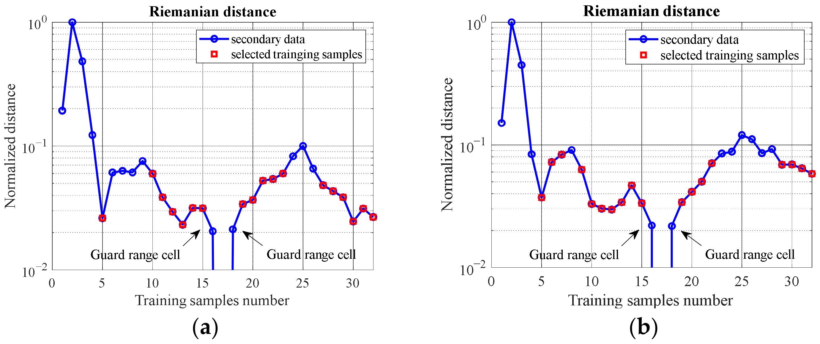
The Riemannian distances between the CUT and other range cells are illustrated in Figure 7. As described in Table 2, the injected targets were distributed in the positive and negative broadened areas separately. For target 1 and target 2, the clutter ridge with the negative Doppler frequency was used as the auxiliary channels, while the clutter ridge with the positive Doppler frequency was used for target 3 and target 4. The targets were in the 17th range cell and this range cell was chosen as the reference. The first three range cells were in the blind zone and could be ignored. The 16th and 18th range cells were set as guard cells. In order to facilitate the comparison with the conventional JDL algorithm, in which the local process region consists of three doppler bins and three beam bins, L was set was 18. Range cells that had a lower Riemannian distance were selected as training samples, as the points marked with square signs denote in Figure 7.

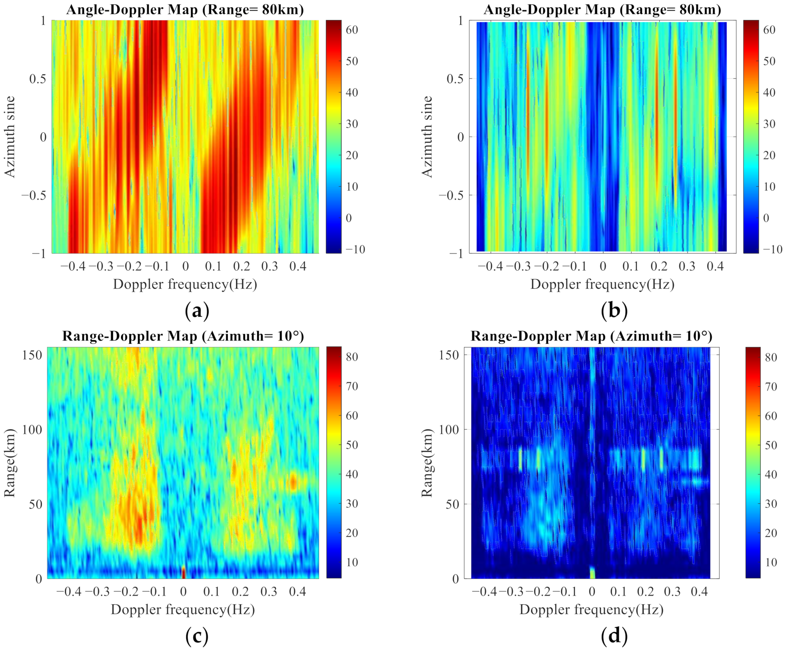
The angle-Doppler and range-Doppler maps are demonstrated in Figure 8. Figure 8b,d denotes the angle-Doppler map and range-Doppler map after clutter suppression, respectively. Compared with Figure 8a,c, processed using 2-dimensional fast Fourier transform and digital beamforming (FFT–DBF) and set as the reference, it is obvious that the broadened first-order sea clutter has been suppressed and targets submerged in the clutter appear.

$${\mathrm{SCNR}}_{\mathrm{Improve}}={\mathrm{SCNR}}_{\mathrm{after}}-{\mathrm{SCNR}}_{\mathrm{before}}\hspace{1em}\left(\mathrm{dB}\right).$$

(41)

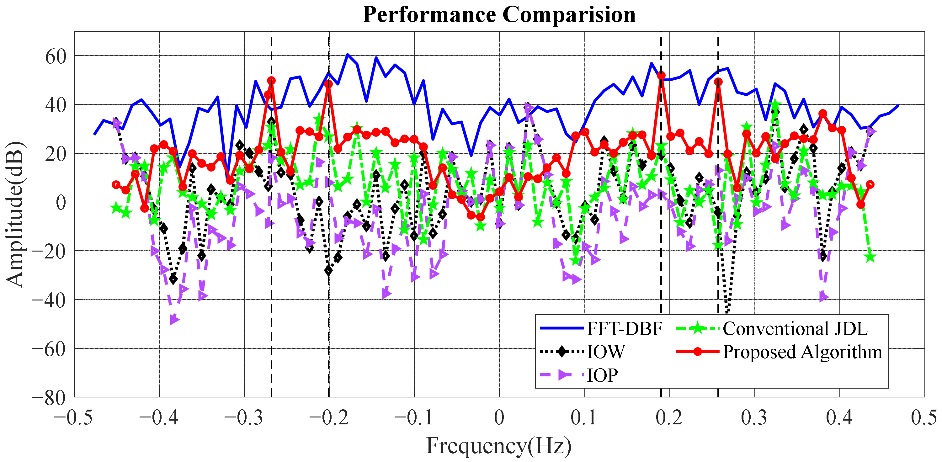
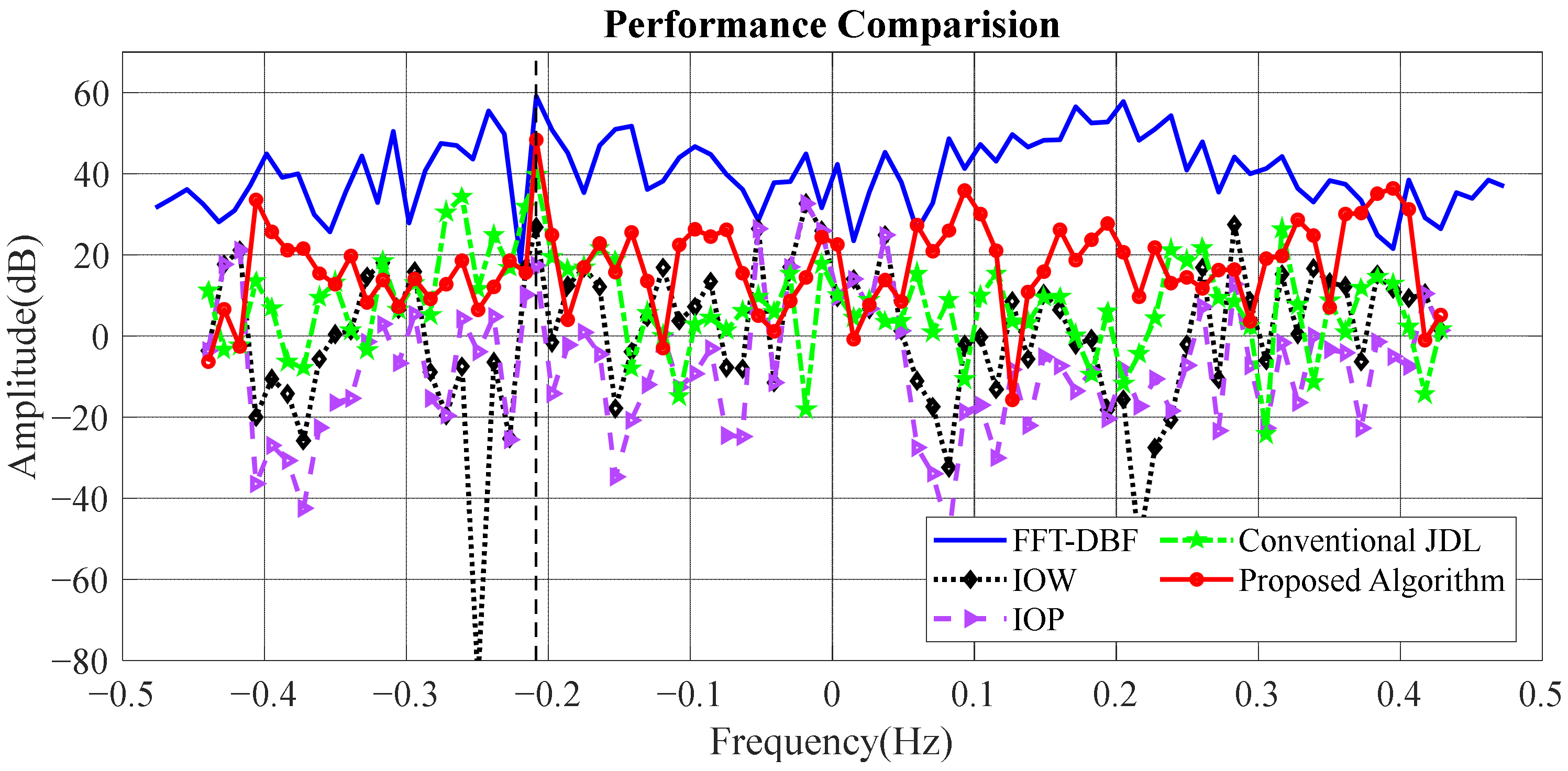
Figure 9 illustrates the comparison of Doppler profiles with simulated targets between the existing clutter-suppression algorithms (conventional JDL [7], IOW [8], IOP [9]) and the proposed algorithm. The FFT-DBF method was set as the reference. The dashed vertical lines represent the Doppler frequency of the injected targets. For all four injected targets, the proposed algorithm worked well. The conventional JDL failed with target 4, the IOW failed with target 2 and target 4, and the IOP algorithm failed with target 3. The average attenuation of the spreading sea clutter was about 25 dB, while the targets almost maintained power for the proposed algorithm. In addition, the proposed algorithm does not introduce frequency estimation deviation, while the other three algorithms will encounter frequency estimation deviation.

The SCNR improvement, which indicates the improvement of the SCNR after clutter suppression, is introduced to quantitatively evaluate the performance of different algorithms. The expression of SCNR improvement is as follows.

For HFSWR, it has a high Doppler frequency resolution and the range resolution is relatively poor, so unlike airborne radar, the Doppler profile is often used to show the performance of clutter suppression. In this paper, the SCNR improvement was calculated based on the Doppler profile. As Equation (40) denotes, $P_s$ is calculated as the power of the target’s Doppler bin. $P_{c+n}$ is calculated as the average power of several Doppler bins around the target.

The results are illustrated in

Table 3. Signal-to-clutter-plus-noise ratio (SCNR) improvement.

Algorithm	SCNR Improvement (dB)
	Simulated Target 1	Simulated Target 2	Simulated Target 3	Simulated Target 4
Conventional JDL	22.03	18.07	16.75	−24.16
IOW	33.09	−27.87	14.00	−9.53
IOP	29.02	18.85	8.64	18.32
Proposed algorithm	27.51	26.07	27.26	24.63

. For the simulated targets, the proposed algorithm had the highest average SCNR improvement. The average SCNR improvement reached about 26 dB. When the target and the first-order sea clutter became close to each other (target 2 and target 4), the IOW algorithm failed due to target gain loss. The IOP algorithm also suffered from performance degradation. The conventional JDL algorithm failed for target 4. Fortunately, the proposed algorithm was robust and had good clutter suppression performance while retaining the target gain.

4.2. Measured Data with Real Target

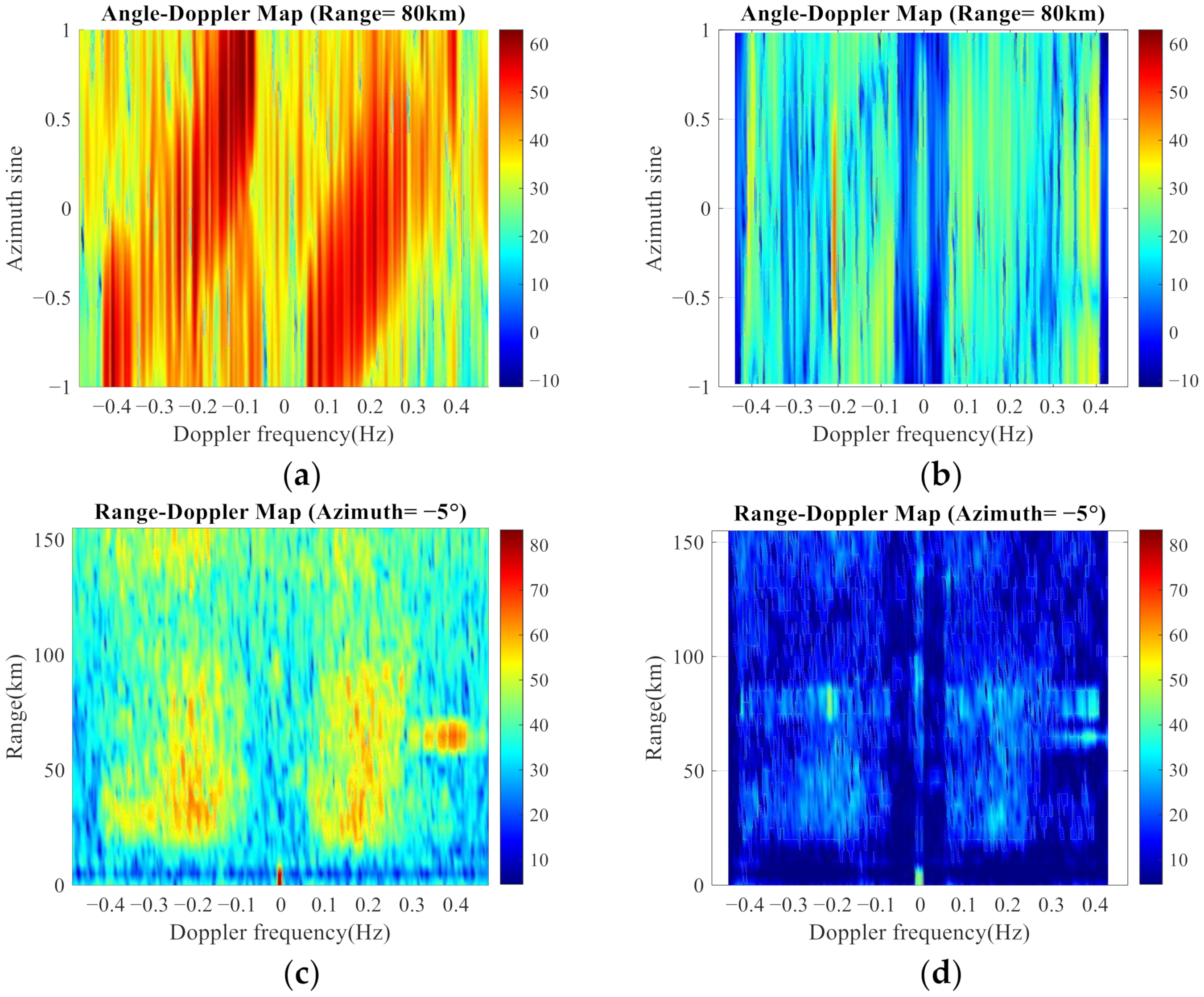
In the recorded measured data, there was a non-cooperative target of a passenger liner. The parameters of this target were: range 78 km, azimuth $-5°$, and radial velocity 5.68 m/s with the corresponding Doppler frequency of −0.2 Hz [3]. The proposed algorithm was used to suppress the clutter and the results are shown in Figure 10. Figure 10b,d illustrates the angle-Doppler map and range-Doppler map after clutter suppression, respectively. Figure 10a shows the initial angle-Doppler map and Figure 10c illustrates the initial range-Doppler map. The training samples used were the same as the selected samples in Figure 7a.

Figure 11 shows the comparison of Doppler profiles between the existing clutter-suppression algorithms. All four algorithms could suppress the broadening first-order sea clutter, but all of them suffered target energy attenuation. The average attenuation of the spreading sea clutter was about 25 dB, while the real target energy attenuation was about 5 dB. The other three algorithms had more obvious attenuation of clutter energy, but at the same time, the energy attenuation of the target became more serious. The target’s SCNR improvement was about 11.54 dB (conventional JDL), 8.51 dB (IOW), 13.91 dB (IOP), and 15.75 dB (proposed algorithm), separately.

5. Discussion

The proposed auxiliary channel STAP algorithm utilizes prior knowledge of the first-order sea clutter and presents an auxiliary channel selection approach. Unlike the conventional JDL algorithm, which has no special requirements for the distribution of clutter in the spatial and frequency domain, the GSC-structure STAP method is suitable for scenario where clutter has a specific spatial or temporal distribution, particularly for mobile platforms where the distribution of ground clutter or sea clutter can be obtained by the system parameters. The proposed training sample selection method can also be extended to other STAP algorithms where the clutter is not homogenous and training samples need to be selected.

6. Conclusions

In this paper, an auxiliary channel STAP algorithm was presented for suppressing the spreading first-order sea clutter in shipborne HFSWR. To obtain better clutter suppression results, this paper improved the STAP algorithm from two aspects. First, a method for selecting auxiliary channels was presented, which employs the knowledge of the space–time distribution of the first-order sea clutter; second, to deal with the heterogeneity of the clutter in range dimension and obtain an accurate estimation of the CCM, a training sample selection method was proposed based on the Riemannian distance between the CUT and other range cells. The range cells that were more similar to the CUT were selected. The performance of the proposed algorithm was evaluated with the measured data. Results showed that for the simulated targets, there was average of 26 dB SCNR improvement after conducting the proposed clutter suppression algorithm, and for the real target, the SCNR improvement reached 16 dB. Compared with FFT–DBF, IOW, IOP, and the conventional JDL algorithm, the proposed algorithm had a better performance when evaluating by the SCNR improvement for both the simulated and real targets, which indicates that the proposed algorithm is effective and superior.

References

- Gao, X.; Zong, C. Ship target detection for HF groundwave shipborne OTH radar. IEE Proc. Radar Sonar Navig. 1999, 146, 305–311. [Google Scholar] [CrossRef]
- Xie, J.; Yuan, Y.; Liu, Y. Experimental analysis of sea clutter in shipborne HFSWR. IEE Proc. Radar Sonar Navig. 2001, 148, 67–71. [Google Scholar] [CrossRef]
- Xie, J.; Yuan, Y.; Liu, Y. Suppression of sea clutter with orthogonal weighting for target detection in shipborne HFSWR. IEE Proc. Radar Sonar Navig. 2002, 149, 39–44. [Google Scholar] [CrossRef]
- Sun, M.; Xie, J.; Hao, Z.; Yi, C. Target detection and estimation for shipborne HFSWR based on oblique projection. In Proceedings of the 2012 IEEE 11th International Conference on Signal Processing, Beijing, China, 21–25 October 2012; pp. 386–389. [Google Scholar]
- Gupta, A.; Fickenscher, T. Sea clutter canceller for shipborne HF surface wave radar. In Proceedings of the 2011 International ITG Workshop on Smart Antennas, Aachen, Germany, 24–25 February 2011; pp. 1–4. [Google Scholar]
- Lesturgie, M. Use of STAP techniques to enhance the detection of slow targets in shipborne HFSWR. In Proceedings of the 2003 International Conference on Radar (IEEE Cat. No.03EX695), Adelaide, Australia, 3–5 September 2003; pp. 504–509. [Google Scholar]
- Ji, Z.; Yi, C.; Xie, J.; Li, Y. The Application of JDL to Suppress Sea Clutter for Shipborne HFSWR. Int. J. Antennas Propag. 2015, 2015, 1–6. [Google Scholar] [CrossRef]
- Yi, C.; Ji, Z.; Xie, J.; Sun, M.; Li, Y. Sea clutter suppression method for shipborne high-frequency surface-wave radar. IET Radar Sonar Navig. 2016, 10, 107–113. [Google Scholar] [CrossRef]
- Yi, C.; Ji, Z.; Kirubarajan, T.; Xie, J.; Hu, B. An Improved Oblique Projection Method for Sea Clutter Suppression in Shipborne HFSWR. IEEE Geosci. Remote Sens. Lett. 2016, 13, 1089–1093. [Google Scholar] [CrossRef]
- Zhu, Y.; Wei, Y.; Zhu, K. Sea clutter suppression for shipborne HFSWR using joint sparse recovery-based STAP. Electron. Lett. 2016, 52, 1067–1069. [Google Scholar] [CrossRef]
- Guo, L.; Yang, Q.; Deng, W. Suppression of sea clutter with modified joint domain localized algorithm in shipborne HFSWR. In Proceedings of the 2016 CIE International Conference on Radar (RADAR), Guangzhou, China, 10–13 October 2016; pp. 1–4. [Google Scholar]
- Guo, L.; Zhang, X.; Yao, D.; Yang, Q.; Bai, Y.; Deng, W. A Single-Dataset-Based Pre-Processing Joint Domain Localized Algorithm for Clutter-Suppression in Shipborne High-Frequency Surface-Wave Radar. Sensors 2020, 20, 3773. [Google Scholar] [CrossRef] [PubMed]
- Fa, R.; De Lamare, R.C. Reduced-rank STAP algorithms using joint iterative optimization of filters. IEEE Trans. Aerosp. Electron. Syst. 2011, 47, 1668–1684. [Google Scholar] [CrossRef]
- Griffiths, L.; Jim, C. An alternative approach to linearly constrained adaptive beamforming. IEEE Trans. Antennas Propag. 1982, 30, 27–34. [Google Scholar] [CrossRef] [Green Version]
- Fabrizio, G.A.; Gershman, A.B.; Turley, M.D. Robust adaptive beamforming for HF surface wave over-the-horizon radar. IEEE Trans. Aerosp. Electron. Syst. 2004, 40, 510–525. [Google Scholar] [CrossRef]
- Xianrong, W.; Feng, C.; Hengyu, K. Sporadic-E ionospheric clutter suppression in HF surface-wave radar. In Proceedings of the IEEE Internatinal Radar Conference, Arlington, VA, USA, 9–12 May 2005; pp. 742–746. [Google Scholar]
- Xianrong, W.; Hengyu, K.; Biyang, W. Adaptive ionospheric clutter suppression based on subarrays in monostatic HF surface wave radar. IEE Proc. Radar Sonar Navig. 2005, 152, 89–96. [Google Scholar] [CrossRef]
- Zhang, X.; Yang, Q.; Yao, D.; Deng, W. Main-lobe cancellation of the space spread clutter for target detection in HFSWR. IEEE J. Sel. Top. Signal Process. 2015, 9, 1632–1638. [Google Scholar] [CrossRef]
- Yao, D.; Zhang, X.; Yang, Q.; Deng, W. An Improved Spread Clutter Estimated Canceller for Main-Lobe Clutter Suppression in Small-Aperture HFSWR. IEICE Trans. Fundam. Electron. Commun. Comput. Sci. 2018, 101, 1575–1579. [Google Scholar] [CrossRef]
- Zhang, J.; Deng, W.; Zhang, X.; Yang, Q. Improved main-lobe cancellation method for space spread clutter suppression in HFSSWR. In Proceedings of the 2018 IEEE Radar Conference (RadarConf18), Oklahoma City, OK, USA, 23–27 April 2018; pp. 0197–0201. [Google Scholar]
- Zhang, X.; Yao, D.; Yang, Q.; Dong, Y.; Deng, W. Knowledge-Based Generalized Side-Lobe Canceller for Ionospheric Clutter Suppression in HFSWR. Remote Sens. 2018, 10, 104. [Google Scholar] [CrossRef] [Green Version]
- Yao, D.; Deng, W.; Zhang, X.; Yang, Q.; Zhang, J.; Li, J. Main-lobe clutter suppression algorithm based on rotating beam method and optimal sample selection for small-aperture HFSWR. IET Radar Sonar Navig. 2019, 13, 1162–1170. [Google Scholar] [CrossRef]
- Zhang, J.; Zhang, X.; Deng, W.; Guo, L.; Yang, Q. A Novel Main-Lobe Cancellation Method Based on a Single Notch Space Filter and Optimized Correlation Analysis Strategy. Int. J. Antennas Propag. 2019, 2019, 1–11. [Google Scholar] [CrossRef]
- Klemm, R. Adaptive airborne MTI: An auxiliary channel approach. IEE Proc. F Commun. Radar Signal Process. 1987, 134, 269–276. [Google Scholar] [CrossRef]
- Zhang, W.; He, Z.; Li, J.; Liu, H. Multiple-input–multiple-output radar multistage multiple-beam beamspace reduced-dimension space-time adaptive processing. IET Radar Sonar Navig. 2013, 7, 295–303. [Google Scholar] [CrossRef]
- Zhang, W.; He, Z.; Li, J.; Liu, H.; Sun, Y. A method for finding best channels in beam-space post-Doppler reduced-dimension STAP. IEEE Trans. Aerosp. Electron. Syst. 2014, 50, 254–264. [Google Scholar] [CrossRef]
- Luo, C.; He, Z.; Li, J.; Zhang, W.; Xia, W. A modified dimension-reduced space-time adaptive processing method. In Proceedings of the 2014 IEEE Radar Conference, Cincinnati, OH, USA, 19–23 May 2014; pp. 0724–0728. [Google Scholar]
- Zhang, W.; He, Z.; Li, J.; Li, C. Beamspace reduced-dimension space–time adaptive processing for multiple-input multiple-output radar based on maximum cross-correlation energy. IET Radar Sonar Navig. 2015, 9, 772–777. [Google Scholar] [CrossRef]
- Li, R.; Li, J.; Zhang, W.; He, Z. Reduced-dimension space-time adaptive processing based on angle-Doppler correlation coefficient. EURASIP J. Adv. Signal Process 2016, 2016, 97. [Google Scholar] [CrossRef] [Green Version]
- Wei, Z.; Zishu, H.; Huiyong, L.; Jun, L.; Xiang, D. Beam-space reduced-dimension space-time adaptive processing for airborne radar in sample starved heterogeneous environments. IET Radar Sonar Navig. 2016, 10, 1627–1634. [Google Scholar] [CrossRef]
- Wen, C.; Tao, M.; Peng, J.; Wu, J.; Wang, T. Clutter suppression for airborne FDA-MIMO radar using multi-waveform adaptive processing and auxiliary channel STAP. Signal Process. 2019, 154, 280–293. [Google Scholar] [CrossRef]
- Zhang, W.; Han, M.; He, Z.; Li, H. Data-dependent reduced-dimension STAP. IET Radar Sonar Navig. 2019, 13, 1287–1294. [Google Scholar] [CrossRef]
- Barrick, D.E.; Headrick, J.M.; Bogle, R.W.; Crombie, D.D. Sea backscatter at HF: Interpretation and utilization of the echo. Proc. IEEE 1974, 62, 673–680. [Google Scholar] [CrossRef]
- Sun, H.; Guo, X.; Lu, Y.; Lesturgie, M. Estimation of the ocean clutter rank for HF/ VHF radar space-time adaptive processing. IET Radar Sonar Navig. 2010, 4, 755–763. [Google Scholar] [CrossRef]
- Junhao, X.; Zhongbao, W.; Zhenyuan, J.; Taifan, Q. High-Resolution Ocean Clutter Spectrum Estimation for Shipborne HFSWR Using Sparse-Representation-Based MUSIC. Ocean. Eng. IEEE J. 2015, 40, 546–557. [Google Scholar] [CrossRef]
- Ishimaru, A. Wave Propagation and Scattering in Random Media; Academic Press: New York, NY, USA, 1978; Volume 2. [Google Scholar]
- Barrick, D.; Snider, J. The statistics of HF sea-echo Doppler spectra. IEEE J. Ocean. Eng. 1977, 2, 19–28. [Google Scholar] [CrossRef]
- Zhang, J.; Zhang, X.; Deng, W.; Ye, L.; Yang, Q.J.R.S. A Geometric Barycenter-Based Clutter Suppression Method for Ship Detection in HF Mixed-Mode Surface Wave Radar. Remote Sens. 2019, 11, 1141. [Google Scholar] [CrossRef] [Green Version]
- Barbaresco, F. Interactions between symmetric cone and information geometries: Bruhat-tits and siegel spaces models for high resolution autoregressive doppler imagery. In Proceedings of the LIX Fall Colloquium on Emerging Trends in Visual Computing, Palaiseau, France, 18–20 November 2008; pp. 124–163. [Google Scholar]
- Reed, I.S.; Mallett, J.D.; Brennan, L.E. Rapid Convergence Rate in Adaptive Arrays. IEEE Trans. Aerosp. Electron. Syst. 1974, AES-10, 853–863. [Google Scholar] [CrossRef]
Figure 1.
Framework of auxiliary channel space–time adaptive processing (STAP).
Figure 3.
Range-Doppler map and angle-Doppler map of measured data. (a) Range-Doppler map, the dashed line represents the spreading region of the first-order sea clutter; (b) Angle-Doppler map, the dashed line denotes the clutter ridge.
Figure 4.
Sketch map of the main channel and auxiliary channels for shipborne high frequency surface wave radar (HFSWR).
Figure 5.
The description of the clutter ridge. (a) Angle-Doppler map, the dashed-line represents the theoretical clutter ridge. (b) The extracted clutter ridge when all beam channels within 3 dB less than the maximum value are selected for a determined Doppler frequency. (c) The extracted clutter ridge when three beam channels are selected for a determined Doppler frequency.
Figure 6.
The correlation coefficients between and .
Figure 7.
Riemannian distance between the cell under test (CUT) and other range cells (the points marked with square sign represent the selected training samples). (a) Negative Doppler frequency region (for targets 1 and targets 2). (b) Positive Doppler frequency region (for target 3 and target 4).
Figure 8.
Angle-Doppler map and range-Doppler map before and after clutter suppression. (a) Angle-Doppler map before clutter suppression. (b) Angle-Doppler map after clutter suppression. (c) Range-Doppler map before clutter suppression. (d) Range-Doppler map after clutter suppression.
Figure 9.
Comparison of Doppler profiles of the simulated targets between different algorithms.
Figure 10.
Figure 11.
Comparison of Doppler profiles of the real target between different algorithms.