
MFANet: A Multi-Level Feature Aggregation Network for Semantic Segmentation of Land Cover


1
Collaborative Innovation Center on Atmospheric Environment and Equipment Technology, Nanjing University of Information Science and Technology, Nanjing 210044, China
2
Jiangsu Key Laboratory of Big Data Analysis Technology, Nanjing University of Information Science and Technology, Nanjing 210044, China
*
Author to whom correspondence should be addressed.
Remote Sens. 2021, 13(4), 731; https://0-doi-org.brum.beds.ac.uk/10.3390/rs13040731
Submission received: 6 January 2021
/
Revised: 8 February 2021
/
Accepted: 11 February 2021
/
Published: 17 February 2021
(This article belongs to the Special Issue Classification and Feature Extraction Based on Remote Sensing Imagery)
Abstract
:Detailed information regarding land utilization/cover is a valuable resource in various fields. In recent years, remote sensing images, especially aerial images, have become higher in resolution and larger span in time and space, and the phenomenon that the objects in an identical category may yield a different spectrum would lead to the fact that relying on spectral features only is often insufficient to accurately segment the target objects. In convolutional neural networks, down-sampling operations are usually used to extract abstract semantic features, which leads to loss of details and fuzzy edges. To solve these problems, the paper proposes a Multi-level Feature Aggregation Network (MFANet), which is improved in two aspects: deep feature extraction and up-sampling feature fusion. Firstly, the proposed Channel Feature Compression module extracts the deep features and filters the redundant channel information from the backbone to optimize the learned context. Secondly, the proposed Multi-level Feature Aggregation Upsample module nestedly uses the idea that high-level features provide guidance information for low-level features, which is of great significance for positioning the restoration of high-resolution remote sensing images. Finally, the proposed Channel Ladder Refinement module is used to refine the restored high-resolution feature maps. Experimental results show that the proposed method achieves state-of-the-art performance 86.45% mean IOU on LandCover dataset.
1. Introduction
Remote sensing images and image processing technology have been widely used in land description and change detection in urban and rural areas. Detailed information about land utilization/cover is a valuable resource in many fields [1]. Semantic segmentation in aerial orthophotos is vitally important for the detection of buildings, forests, water and their variations, such as research on urbanization speed [2], deforestation [3] and other man-made changes [4].
There were still some defects in existing land cover classification models. Among the traditional remote sensing image classification methods, the maximum likelihood (ML) method [5] was widely used. This method obtained the mean value and variance of each category through the statistics and calculation of the region of interest, thereby determining the corresponding classification functions. Then each pixel in the image was substituted into the classification function of each category, and the category with the largest return value was regarded as the attribution category of the scanned pixel. Other similar methods relied on the ability of trainers to perform spectral discrimination on the image feature space. However, with the development of remote sensing technology, image resolution continued to be improved, and spectral features were becoming more abundant, which led to the problems that spectral classes may have small difference and the same classes may present big difference. It was often insufficient to accurately extract target objects by spectral features. The classification algorithms based on machine learning such as support vector machine [6], artificial shallow neural network [7], decision tree [8] and random forest [9] were not suitable for massive data. When they were used for classification, the input features only underwent a few linear or non-linear transformations, and the rich structural information and complex regular information were often not well described by above methods. Especially for the high-resolution remote sensing images with large difference in features and complex spectral texture information, the above classification results were unsatisfactory.
For the land cover analysis [10], aerial orthophotos are used widely. There are various ways of land occupation, among which the size of the land covered by the buildings varies greatly, and the buildings are easily confused with greenhouses in terms of appearance in orthographic projection. Woodland is the land covered with trees standing in close proximity, and the area covered with single trees and orchards is difficult to be distinguished from the woodland. Moreover, there are many types of planted trees, which are different in irrigation methods and soil types. Water is divided into flowing water and stagnant water, and ponds and pools are included and ditches and riverbeds are excluded. These characteristics make it very difficult to extract features from remote sensing images when feature extraction is the basis of classification. Besides, the above traditional methods [5,6,7,8,9] usually required manual participation in parameter selection and feature selection, which further increased the difficulty of feature extraction. In addition, remote sensing images, especially aerial images, are developing in the direction of higher resolution and larger time and space span, and problem that the same objects may have different spectrum whereas different objects may share the same spectrum becomes more often. In summary, traditional remote sensing image classification methods had limited capabilities of feature extraction and poor generalization, and could not achieve accurate pixel-level classification of remote sensing images.
In the field of deep learning, since Long et al. [11] proposed a fully convolutional neural network (FCN) in 2015, many subsequent FCN-based deep convolutional neural networks have achieved end-to-end pixel-level classification. For example, Ronneberger et al. [12] proposed a U-shaped network (U-Net) that could simultaneously obtain context information and location information. The pyramid pooling module proposed by Zhao et al. [13] could aggregate the contextual information of different regions, thereby improving the ability to obtain global information. Chen et al. [14] used cascaded or parallel atrous convolutions to capture multi-scale context by using different atrous rates. Yu et al. [15] proposed a Discriminative Feature Network (DFN) to solve the problems of intra-class inconsistency and inter-class indistinction. In Huan et al.’s work [16], the features of different levels from the main network and the semantic features from the auxiliary network were dimensionally reduced by principal component analysis (PCA), respectively. And then these features were fused to output the classification results. In Yakui et al.’s work [17], the efficiency of information dissemination was improved by adding the nonlinear combination of the same level features, and the fusion of different layer features was used to achieve the goal of accurate target location. Compared with traditional remote sensing image classification methods such as ML and SVM based on the single source data, deep learning methods learn to extract the main features rather than designed by experts, which is more robust in complex and changeable situations. In addition, deep learning methods greatly enhance the capabilities of feature extraction and generalization, and could achieve more accurate pixel-level classification; therefore, they are more suitable for high-resolution remote sensing image classification.
With the use of unmanned aerial vehicles, aerial image datasets become more and more popular, and they are developing in the direction of high resolution, multi-temporal, and wide coverage. Traditional methods based on hand-made feature extractors and rules have low efficiency and poor scalability when the amount and the variance of data are large. In recent years, convolutional neural networks (CNNs) have played a key role in automatic detection of changes in aerial images [18] [19]. However, the low-level features learned by CNNs are biased toward positioning information, and the high-level features are biased toward semantic information. In the land cover classification model, the model needs to know not only the category, but also the location of the category, so as to complete the land cover classification task, which is actually a semantic segmentation task. There are two common neural network architectures used for semantic segmentation. One is the spatial pyramid pooling style networks, such as Pyramid Scene Parsing Network (PSPNet) [13], ParseNet [20] and Deeplabv2 [21], and the other is the encoder-decoder style networks, such as SegNet [22], Multi-Path Refinement Networks (RefineNet) [23], U-Net [12] and Deeplabv3+ [24]. The former networks could detect incoming features at multiple scales and multiple effective receptive fields by using filters or performing pooling operations, thereby encoding multi-scale context information. The latter networks could capture clearer object boundaries by gradually recovering spatial information. In the land cover classification problem, objects of the same classes vary widely in time and space, but the requirement for multi-scale information of each class is not high.
Since down-sampling operations are usually used in convolutional neural networks to extract abstract semantic features, high-resolution details are easily lost, and some problems e.g. inaccurate details and blurred edges emerge in the segmentation results. There are two mainstream solutions to solve the detail loss of high-resolution image. The first solution is that high-resolution feature maps are used and kept throughout the network. This method requires higher hardware performance, which results in low popularity. The representative networks include convolutional neural fabrics [25] and High Resolution Network (HRNet) [26]. The second solution is that high-resolution detail information are learnt and restored from low-resolution feature maps. This method is used by most semantic segmentation networks such as PSPNet [13], Deeplabv3+ [24] and Densely connected Atrous Spatial Pyramid Pooling (DenseASPP) [27]. However, this scheme needs to recover the lost information and the result is unsatisfactory. Therefore, the land cover classification models based on semantic segmentation still need to be improved in both deep feature extraction and up-sampling feature fusion. In order to solve the above problems, a multi-level feature aggregation network (MFANet) is proposed for land cover segmentation in this work. In terms of deep feature extraction, a Channel Feature Compression (CFC) module is proposed. Although the structure of CFC module is similar to Squeeze-and-Excitation (SE) module [28], their functions are different. The SE module is embedded in the building block unit of the original network structure, aiming to improve the network’s presentation ability by enabling it to perform dynamic channel feature recalibration. While the proposed CFC module placed in the middle of the encoder and the decoder, compresses and extracts the deep global features of high-resolution remote sensing images in the channel direction, and provides more accurate global and semantic information for the subsequent up-sampling process. This alleviates the phenomenon of the same thing with different spectrum to a certain extent. In terms of up-sampling feature fusion, we propose another two modules, Multi-level Feature Attention Upsample (MFAU) and Channel Ladder Refinement (CLR). The MFAU module is used to restore high-resolution details. The MFAU module uses multi-level features, rather than only two levels of features are used in traditional up-sampling modules like Global Attention Upsample (GAU) [29] and traditional networks like U-Net [12]. At the same time, each MFAU module also generates a twice-weighted feature combination by performing different convolution and global pooling operations. These two innovations give the MFAU module a powerful ability to recover detailed information for high-resolution remote sensing images. To achieve the purpose of smooth transition to a specific land cover classification task, the proposed Channel Ladder Refinement (CLR) module is placed at the end of the network and gradually refines the restored high-resolution feature maps by decreasing progressively the number of channels.
In general, there are four contributions in our work:
- A channel feature compression module placed at the end of the feature extraction network is proposed to extract the deep global features of high-resolution remote sensing images by compressing or filtering redundant information, and therefore to optimize the learned context.
- A multi-level feature attention upsample module is proposed, and it uses higher-level features to provide guidance information for low-level features, which generates new features. The high-level features further provide guidance information for newly obtained features, and are re-weighted to obtain the latest features. This is of great significance for restoring the positioning of high-resolution remote sensing images.
- This work also proposes a channel ladder refinement module, which is placed before the last up-sampling, with the purpose of gradually refining the restored higher resolution features for any specific land cover classification task.
- A network combines the three modules with the feature extraction network is proposed to achieve the purpose of segmenting high-resolution remote sensing images.
2. Methodology
As the resolution of remote sensing images increases, the detailed information and spatial information of remote sensing images also increases dramatically. As the key to describing land cover, the loss of contextual information means the failure and decline of the models. How to effectively represent contextual information has become an effective means to improve the classification results of the models. At present, the existing models are not very good at recovering the lost spatial details. Therefore, the land cover classification models based on semantic segmentation still need to be improved in deep feature extraction and up-sampling feature fusion.
In this part, the architecture of MFANet is introduced firstly, and then three modules CFC, MFAU, and CLR are described in detail.
2.1. Network Architecture
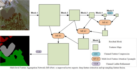
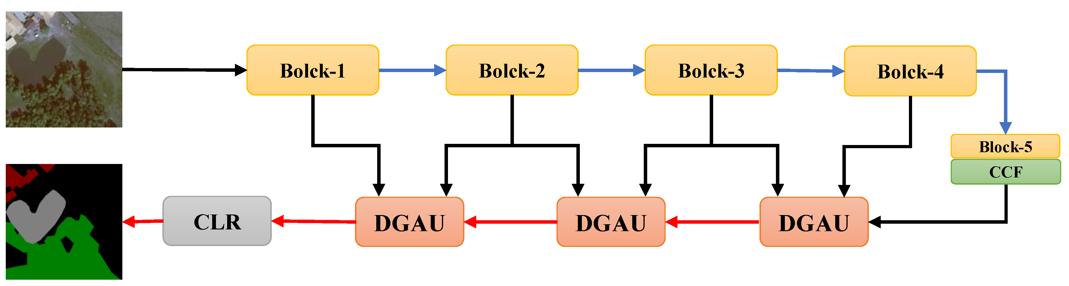
This paper proposes a new semantic segmentation network, and the network structure is shown in Figure 1. Firstly, the proposed CFC is regarded as the central block between the encoder and the decoder. Its function is to extract the deep global features of high-resolution remote sensing images in the channel direction. To a certain extent, it alleviates the phenomena of the same objects with different spectrum and different objects with same spectrum. Secondly, the proposed MFAU module is an improvement of the GAU module proposed in Pyramid Attention Network (PNA) [29]. The GAU module adds a global pooling operator as an accessory to the decoder branch to choose the distinctive multi-resolution feature representations, which is proved to be effective. The features of adjacent stages are not a simple combination, and their different representations and global context information jointly generate a twice-weighted feature combination by performing different operations such as convolution and global pooling. The experimental results show that this operation can better restore the detailed information of the high-resolution remote sensing images. Thirdly, the proposed CLR module is used in the last step of the network to refine the final feature maps.
Combined the proposed CFC, MFAU and CLR, the multi-level feature aggregation network for land cover segmentation is proposed, as shown in Figure 1. ResNet-50 [30] is used as the backbone. Table 1 gives a detailed description of the division of five Blocks from ResNet-50. The Block-1 to Block-4 remain unchanged, and the Block-5 is modified. That is, the last three plain convolutions are replaced with the atrous convolutions with , so the size of final output feature maps of ResNet-50 is 1/16 of the input images. The CFC module is used to collect compressed global context information from the output of the backbone ResNet. In the up-sampling process, combined with the global context, three MFAU modules gradually fuse features from high-level to low-level to recover high-resolution details. The CLR module is utilized to gradually refine the recovered high-resolution feature maps, and generate the final prediction maps after the last up-sampling.
2.2. Channel Feature Compression
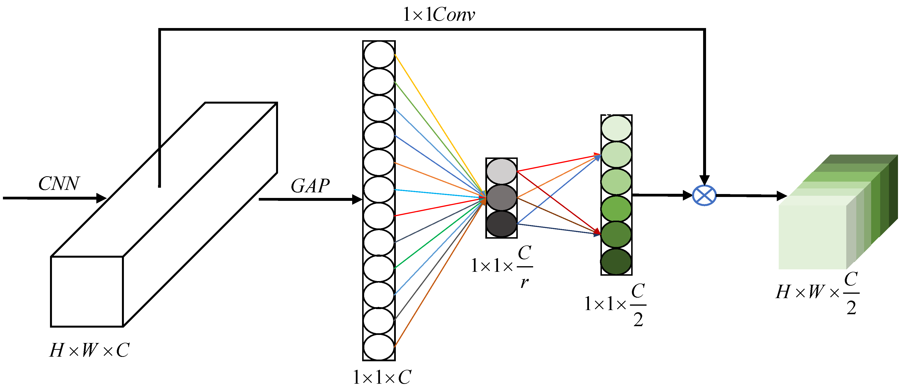
In the land cover classification problem, the objects of the same classes vary widely in different time and space. Therefore, this work mainly considers how to effectively extract deep global features in the channel direction. In this work, the CFC module is regarded as the central block between the encoder and decoder. Its function is to optimize the learned context by compressing or filtering redundant information, and to better extract the deep global features of high-resolution remote sensing images. Hu et al. [28] proposed a SE module, which enhances the learning of convolutional features by explicitly modeling channel interdependence. While the CFC module, as shown in Figure 2, uses a convolutional layer followed by a Batch Normalization (BN) layer to replace a fully connected layer. This operation has two benefits. Firstly, the fully connected layer destroy the spatial structure of images, while the convolutional layer will not. For a semantic segmentation task, we obviously do not want to destroy the spatial structure of the images, so the convolutional layer is first choice. Secondly, the computational process of the convolution is equivalent to the process of the fully connected layer, and the batch normalization layer is followed, so that the update of model parameters during the training is not likely to cause drastic change of the output near the output layer, and the learning of network is more stable.
In this work, ResNet is a feature extraction backbone after removing average the pooling layer, the fully connected layer and the softmax layer. The high-level features learned from the backbone are further processed by a global average pooling to learn global information, so that a weight vector whose length is C is obtained. The vector trains the model to achieve better performance in such a way that the effective feature maps’ weight values become large and the less effective feature maps’ weight values become small, which can be expressed by Equation (1).
where represents the c-th component of the weight vector, which can also be understood as the global average information of the c-th channel of the feature maps.
Through the above operation, the spatial correlation has been decoupled. In order to capture the correlation between channels, the bottleneck formed by two convolutional layers (that is, the dimensionality reduction layer with reduction ratio r) is used to process the entire channel information. This process can be described as the followings:
where the first convolution has convolution kernels, represents the c-th convolution kernel, represents the c-th feature generated after the first convolution, and represents further batch normalization and ReLU nonlinear activation; the second convolution has convolution kernels, represents the c-th convolution kernel, represents the c-th feature generated after the second convolution, and represents the further batch normalization and Sigmoid nonlinear activation. It should also be noted that .
It can be seen from the Equations (2)–(5) that there is another difference from SE module, Double Attention Module [31] and Attention Fusion Block [32] that the CFC module has achieved the goal of the halved number of channels. The reason for this is that as networks become deeper, the number of channels gradually doubles, but there is actually channel redundancy for most tasks. For the land cover classification task, we use ResNet-50 [33,34] as the backbone, but the number of channels in the last convolutional layer has reached 2048. For the semantic segmentation task with four classes, the number of channels is far larger than what is actually needed. The proposed method has two additional benefits. Firstly, the original channel number of the backbone is not changed, so the official pre-trained weights can be easily loaded, which shortens the training time. Secondly, for the subsequent up-sampling feature fusion to restore high-resolution details, it reduces the amounts of calculations and parameters, and reduces hardware requirement.
In order to match the number of channels, the features X followed a convolution are multiplied by the normalized weight channel by channel to complete the recalibration of the original features in the channel dimension. The process can be described by Equations (6) and (7).
where represents the c-th channel component of the final output features of the module.
We can add a CFC module at the end of the backbone. In addition to the common ResNet, we can also use MobileNetv2 [35] as a lightweight backbone. With a little modification to different backbones, we can extract the features of different levels that we need to prepare for the up-sampling process [36].
2.3. Multi-Level Feature Attention Upsample
This work proposes an encoder-decoder style network, which gradually completes the up-sampling feature fusion and restoration through three MFAU modules. The main idea of the MFAU module is to use higher-level features to provide guidance information for low-level features to generate new features, and high-level features further provide guidance information for newly obtained features to obtain the latest features. Compared with the GAU module [29], although the amounts of parameters and calculations of the module have increased, the segmentation effect is significantly improved and the high-resolution details of remote sensing images are better restored.
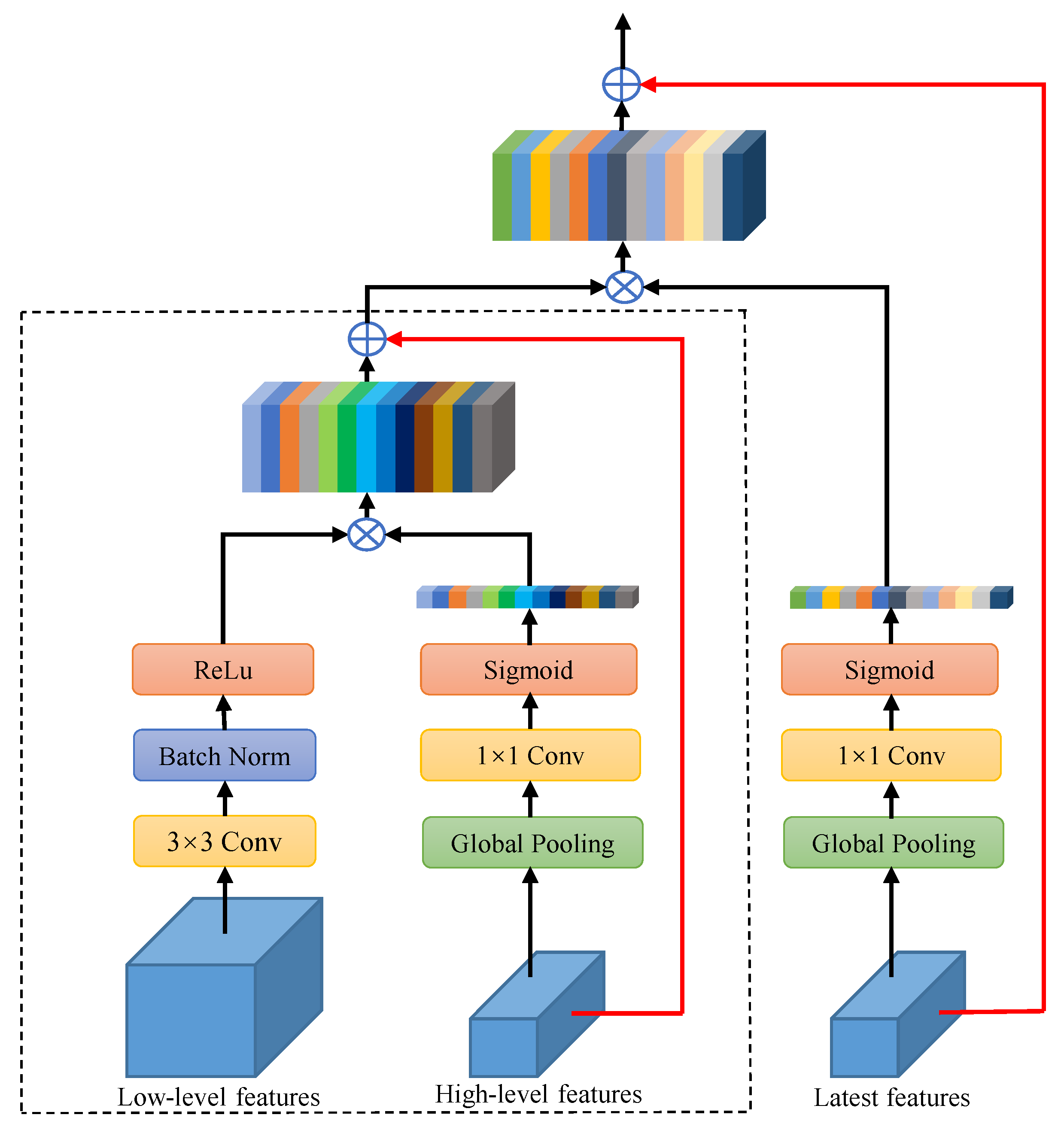
Up-sampling is used to restore the resolution or fix the pixel positioning. This process is very important, and MFAU module is a good implementation for up-sampling. High-level features with rich semantic information can be used to weight low-level features to select precise resolution details, this idea is used twice in the module. The MFAU module is different from general up-sampling modules. It has three inputs (multi-level), two of which are derived from the adjacent levels of the backbone called low-level features and high-level features, respectively. Another is generated by the CFC module or the last MFAU module, and named the latest features. We design that number of channels and the size of the latest features are the same as those of the high-level features. The number of channels of low-level features is 1/2 of that of high-level features, and the length and width are twice the size of high-level features. The module structure is shown in Figure 3.
Most methods try to combine features from adjacent stages to enhance low-level features, regardless of their different representations and global context information. In Li et al.’s work [29], the global pooling operator was added as an accessory module to the decoder branch to select a distinctive multi-resolution feature representation. The idea is adopted and expanded. The features of adjacent stages are not simply combined in this work. Instead, their different representations and global context information are considered by performing different operations such as convolution and global pooling to jointly generate a twice-weighted feature combination. In detail, this operation is divided into two stages. The first stage is shown in the part surrounded by the black dashed line. First, a convolution with batch normalization and ReLU nonlinear activation is performed on the low-level features while keeping the number of channels and the size of the feature maps unchanged. Then, it is then multiplied by a global context vector, which is generated by performing a convolution with Sigmoid nonlinear activation on adjacent high-level features. Finally, the up-sampled high-level features are added to the weighted low-level features. In the second stage, the features generated in the first stage are multiplied by the global context vector generated by the latest features. Finally, the latest features after up sampling are added with the weighted features to get the final output of the module, that is, the next features we want, whose size and channel number are consistent with the low-level features.
If the output of the first stage is regarded as the low-level features, combined with the remaining part, this will become a first stage. In our proposed networks, we use the module three times in the up-sampling process, and the corresponding relationships between input and output in these three modules can be described by Equation (8).
where represents the output of the CFC module. is the output of the i-th MFAU module, that is, the latest features. represents the feature maps generated from the Block-i of the backbone. represents the entire calculation process of the MFAU module.
With this design, the feature maps outputted by Block-3 and the Block-2 are reused. The resolution of the two blocks is respectively 1/8 and 1/4 of the original images, which is a good compromise for both positioning information and semantic information. It is found that this is of great significance for restoring the positioning of high-resolution images.
2.4. Channel Ladder Refinement
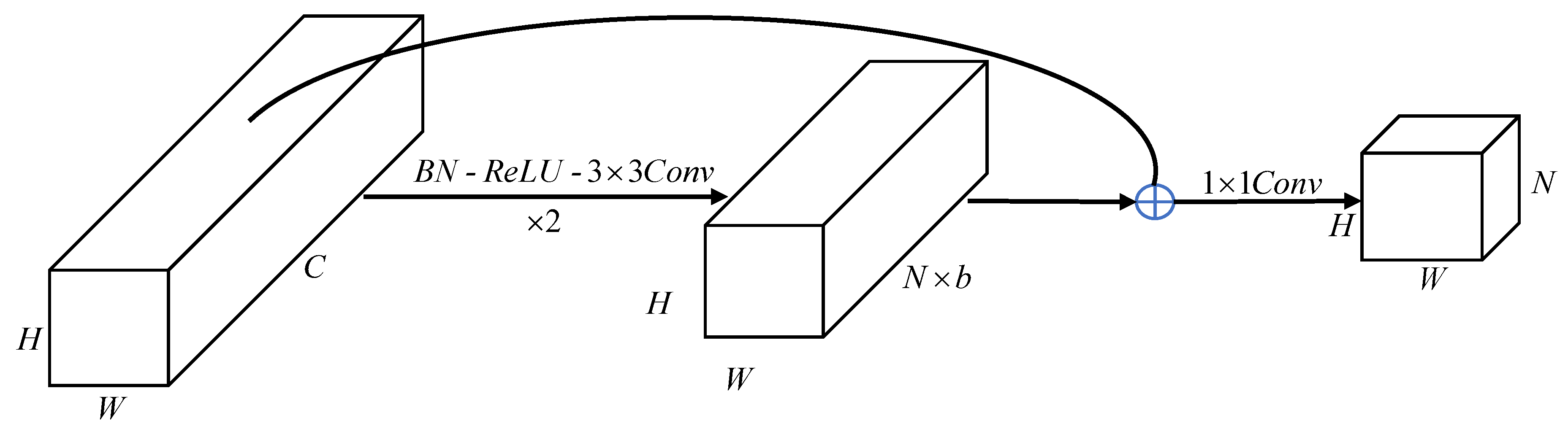
Before the last up-sampling, a Channel Ladder Refinement module is added to gradually refine the restored higher-resolution features. The structure of the module is shown in Figure 4. The first layer of the module is a convolution, we use it to reduce the number of channels to b times as many as the output channels. At the same time, it can also combine information from all channels. Next is a basic residual block from ResNetv2 [37], which can better refine the feature maps. Finally, a convolutional layer is used to further reduce the number of channels. In this way, the number of channels is reduced in two times to achieve the goal of gradually refining the feature map. Compared with the similar Refinement Residual Block (RRB) proposed by DFN [15], the accuracy is improved.
3. Experiment
3.1. Datasets
3.1.1. LandCover Dataset
In order to verify the ability of the proposed model in land cover segmentation task, the LandCover dataset [10] is used. The dataset consists of images selected from aerial photos covering 216.27 square kilometers of land in Poland, a central European country. It is manually labeled with four types of objects: buildings (red), woodland (green), water (grey), and background (black), which are called ground truth, as shown in Figure 5b. The dataset has 33 images with a resolution of 25 cm (about px) and 8 images with a resolution of 50cm (about px).
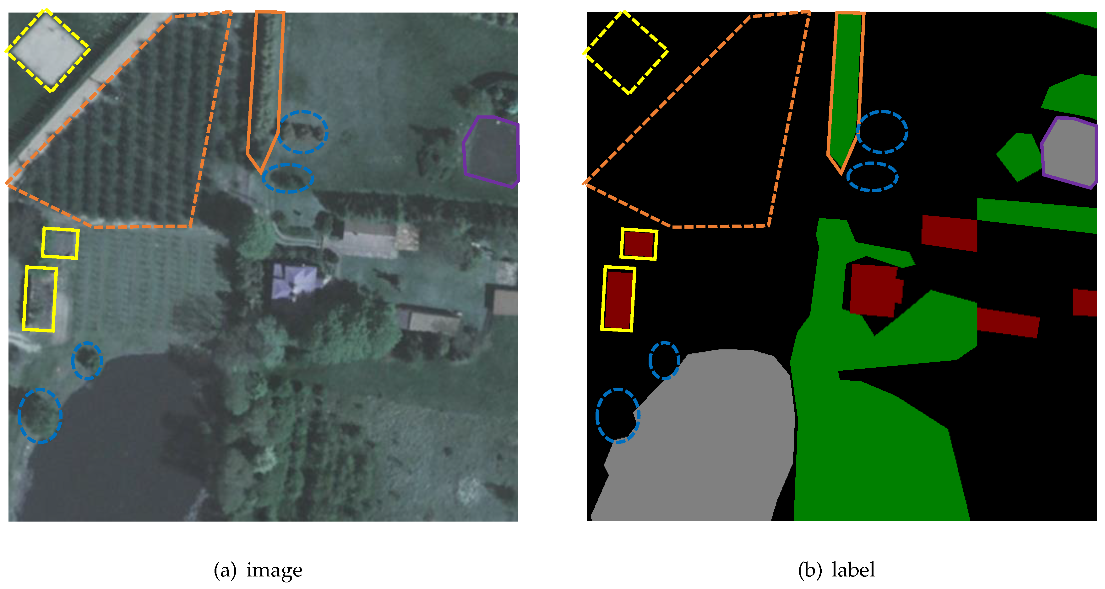
There is difficult in semantic segmentation on this dataset. In addition to the two points of high resolution and multiple time and space mentioned above, there are also strict definitions of four types of objects. Buildings are objects that stand permanently in one place, excluding greenhouses, etc. Wood-land refers to land covered by trees, excluding single trees and orchards. Water include flowing water and stagnant water, but does not include ditches and dry riverbeds. These remote sensing images with orthographic projection are likely to cause indistinguishability in appearance. There is an example is shown in Figure 5. In Figure 5a, the object encircled by a yellow circle is easy to be misclassified as a building in appearance, but it is actually greenhouse and should be classified as the background. The object surrounded by an orange triangle appears to be wood-land, but it is actually a bush and should be classified as the background. The objects encircled by blue ellipses are single trees, and they should be classified as the background. In summary, it is difficult to satisfactorily classify land cover accurately on this dataset.
For the processing of this dataset, all images were cut from left to right and top to bottom without overlapping to the images with px. The images with only one class are eliminated, and then randomly are divided into training set, validation set and test set according to the ratio of 0.7:0.15:0.15.
3.1.2. Aerial Image Segmentation Dataset
The dataset is an aerial image segmentation dataset (AISD) [38] covering six cities, all images are high-resolution RGB orthophotos from Google Maps. The ground truth of Tokyo comes from fine manual annotation, annotated three types of objects: building (red), road (blue), and background (white). The ground truths of Berlin, Chicago, Paris, Potsdam and Zurich are automatically exported from OpenStreetMap (OSM). Affected by factors such as OSM polygons and Google images being independently geo-referenced, the way of annotation is not so detailed compared to manual annotation. For the processing of this dataset, we follow the approach adopted for LandCover.
3.2. Implementation Details
Our implementation is based on the public platform PyTorch. The ‘ploy’ learning rate strategy is used in this work, that is, the current learning rate is equal to the basic learning rate multiplied by . The base learning rate is set to 0.01 and power is set to 0.9. It has been observed that most experiments have almost converged after 200 iterations, so the maximum number of iterations is set to 300. Momentum and weight decay are set to 0.9 and 0.0005, respectively.
Due to limited physical memory on our GPU card, the batch size is set to 4 during training. Considering that the sample imbalance problem may cause some classes to be easily trained, which will dominate the update direction of the gradients, so that the network cannot learn more useful information, and cannot accurately classify each class. Therefore, in this paper we use focal loss [21] to supervise the output of the network, as shown in Equation 9. We adjust the parameters and of focal loss to obtain better performance. That is .
where is the estimated probability of the class k , . K is the maximum value of the class label.
3.3. Ablation Study on LandCover Dataset
In this part, the ablation experiments are organized step by step to reveal the effect of each module on LandCover dataset. For evaluation, we mainly use the mean Pixel Accuracy (mPA) and mean Intersection-over-Union (mIoU) indexes, and show the amounts of parameters and calculations of each network.
3.3.1. Channel Feature Compression
It is suggested that reduction ratio r must be greater than or equal to 2 so as to better filter redundant channel information. Observing the experimental results, as shown in Table 2, it is found that when r=4, the performance is the best, and the amounts of parameters and calculations are also relatively compromised. At the same time, the first row of Table 3 indicates that using the CFC module instead of the SE module increases the mIoU by up to 0.36% but not increases the amounts of parameters and calculations. These results indicate that when the CFC module is regarded as the central block between the encoder and decoder, it can effectively extract the deep global features of high-resolution remote sensing images, optimize the learned context information, and alleviate the phenomenon of different spectra of the same object and the same spectrum of foreign objects to a certain extent. The performance can be attributed to the fact that CFC module enhance the learning of convolution features by explicitly modeling channel interdependence, while compressing redundant features in channel dimension.
3.3.2. Multi-level Feature Attention Upsample
In the up-sampling process, the MFAU modules are used instead of the GAU modules. From the results in the first and third rows of Table 3, the performance is enhanced from 84.59% to 85.66%, an increase of 1.07%. This shows that the MFAU modules can perform up-sampling feature fusion more effectively and better restore high-resolution details than the GAU modules. MFAU takes into account the different representations and global context information of the features of adjacent stages, and generates a twice-weighted feature combination by performing different operations such as convolution and global pooling. This process can be described as two steps. At first, higher-level features provide guidance information for low-level features to generate new features, and then the highest-level features further provide guidance information for the new features. It is of great significance to restore the location of high-resolution remote sensing images.
3.3.3. Channel Ladder Refinement
For the dataset with 4 classes, the output feature maps from the last MFAU module have 64 channels. There are two extreme cases with buffer factors b of 1 and 16. The results are shown in Table 4. It is observed that when b=16, that is, when the number of channels is reduced in the last convolutional layer, the performance is the best. However, considering the amounts of parameters and calculation, a buffer factor of 4 is chosen. At the same time, compared with the first row of Table 3, any of these four results is better than using the RRB module. This is due to a residual block [37] contained in the module, which is used to gradually refine the recovered higher resolution features.
3.3.4. Dilation Ratio of Block-5
Based on reduction ratio r=4 and buffer factor b=16, we conduct further experiments on our networks. In DeepLabv1 [39], the concept of hole convolution was first proposed. The dilated convolution can expand the receptive field without introducing additional parameters. When dilated convolutions at different rates are used continuously, these networks can capture multi-scale context information, which is quite important in many visual tasks [40,41]. However, whether this approach is suitable for feature extraction of remote sensing images is a problem worthy of exploration. Through the experiments, the three convolutions of Block-5 from ResNet-50 use different dilation ratio combinations, and the results are shown in Table 5. When ratios are all 1, that is, without dilated convolutions, the performance is relatively better. This indicates that the dilated convolution is unlikely to be suitable for extracting features from remote sensing images.
Finally, using the configuration obtained from the above experiments, the Mean IoU of our proposed network reaches 86.45%, as shown in Table 3, which is 1.88% higher than the baseline network.
3.4. Comparative Experiment with Other Networks
3.4.1. Comparative Experiment on LandCover
In this part, the proposed method is compared with other semantic segmentation networks. As the experimental results show in Table 6, the performance of the proposed MFANet based on Resnet50 is best. Without pre-training, the performance of MFANet based on MobileNetv2 is better than that of most networks, and the amounts of parameters and calculations are greatly reduced. The performance of MFANet based on ResNet-50 is better than PSPNet and U-Net. In contrast, our network has the least computation and the second largest parameter. In the case of pre-training, MFANet based on ResNet-50 or MobileNetv2 has better performance than other networks such as DeeplabV3, BiSeNet and DenseASPP. Table 7 shows the detailed results for each class of the test set in which all methods’ backbones are loaded with pre-trained weights. By comparison, IoU for each class of our proposed network whether it is based on Resnet50 or MobileNetv2 is better than that of other networks. All of these results show the effectiveness of our proposed network. Moreover, it can be seen from the amounts of parameters and calculation in Table 6 that the performance promotion of our network is not simply at the cost of increasing parameters and computing.
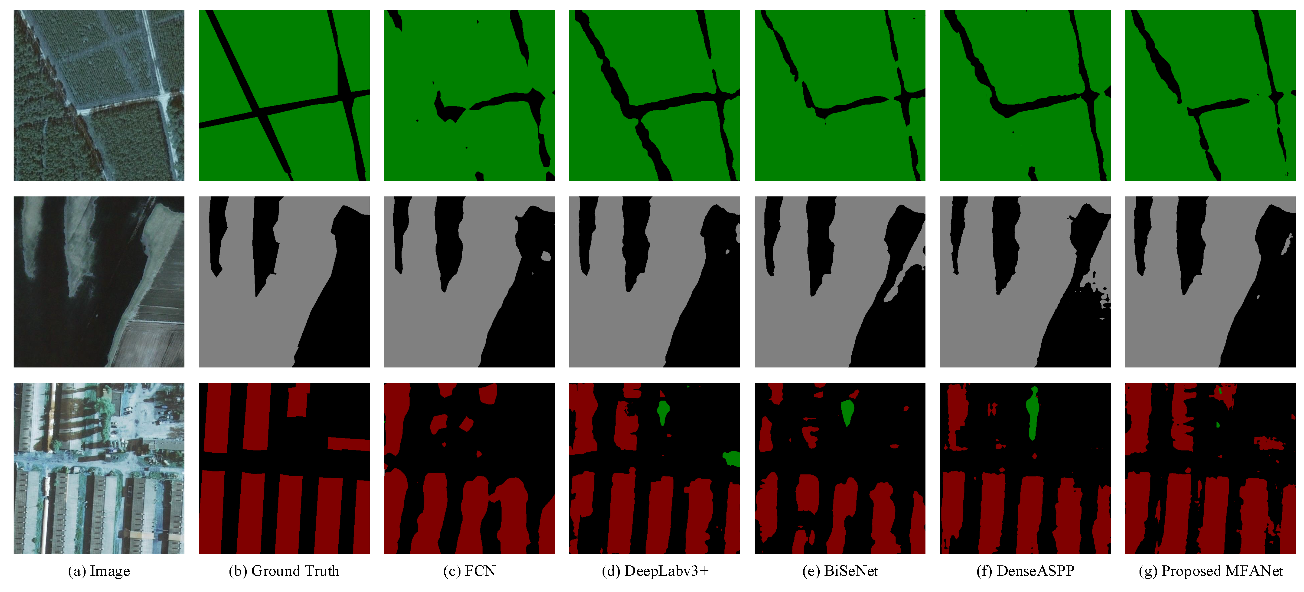
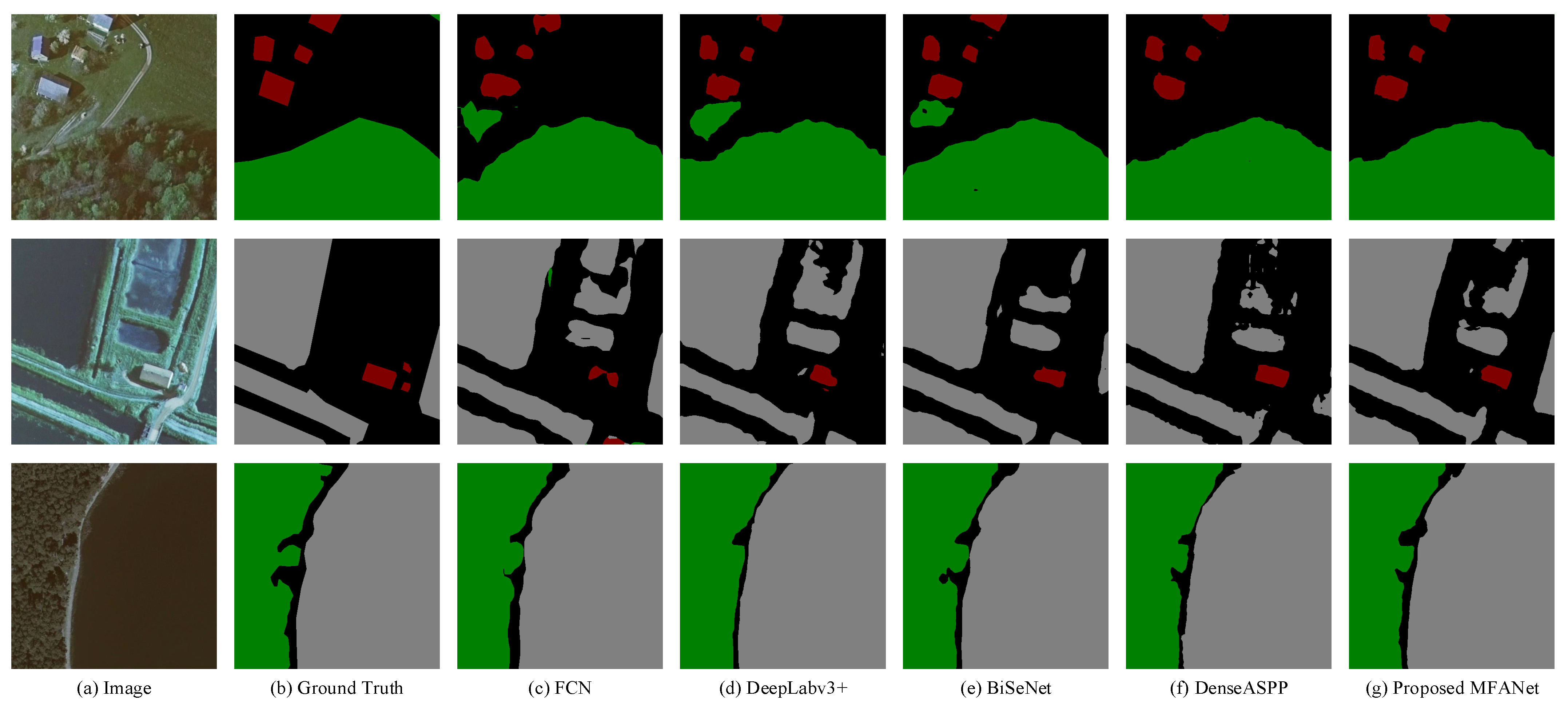
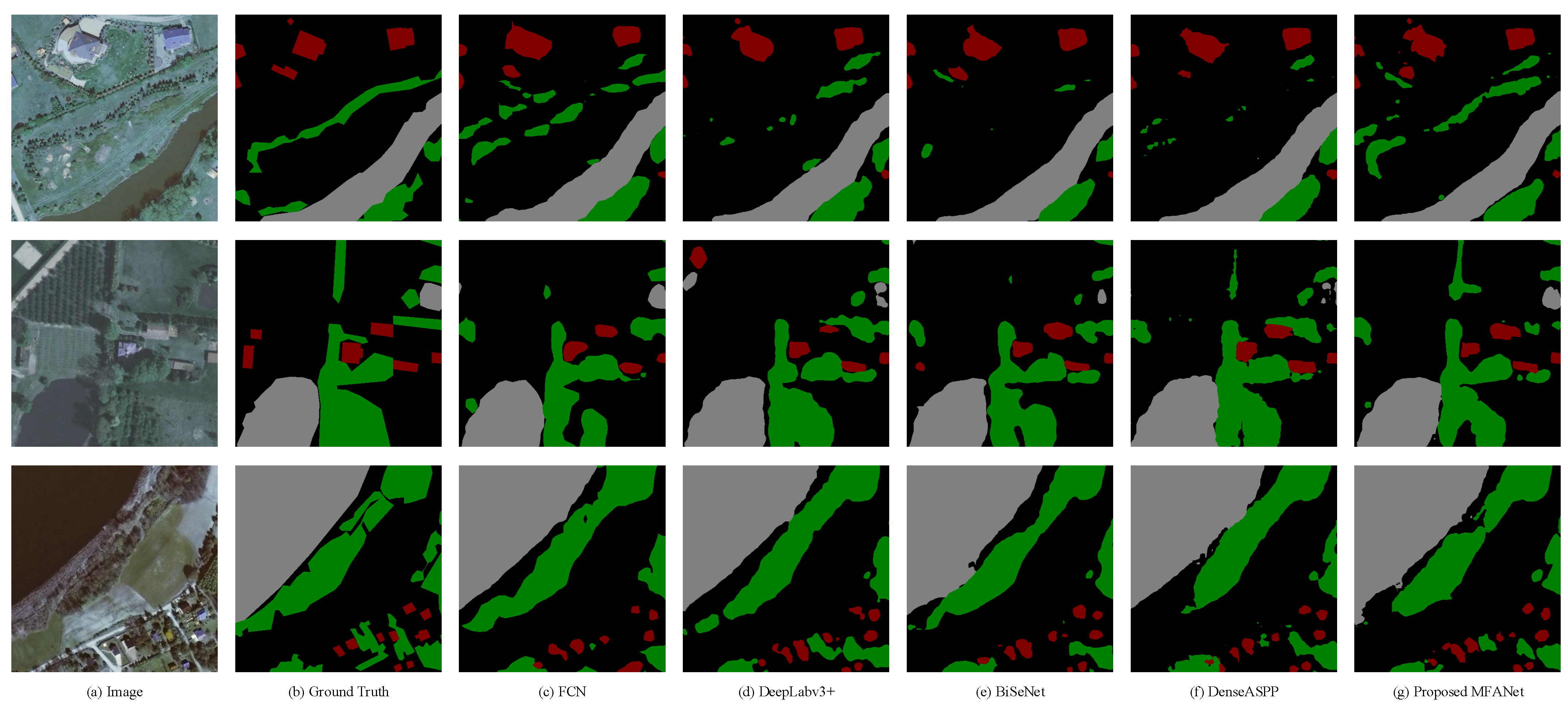
Figure 6, Figure 7 and Figure 8 show several example effects of remote sensing images within different number of classes. Figure 6 shows the prediction results of several images within two classes. It can be seen that whether for woodlands, water or buildings, our result in Figure 6g is closest to ground truth Figure 6b. Figure 7 shows the results of several images within three classes. In the first row, the proposed network removes the distractors. The result shows that our network has an advantage in the identification of distractors. This is due to CCF module enhancing the learning of convolution features by modeling channel interdependence, which alleviates the phenomenon of the same objects with different spectrum and different objects with the same spectrum in remote sensing images to a certain extent. In the second line, our network segments more complete buildings and water at the same time. This MFAU module takes into account the different representations and global context information of the features of adjacent stages to generate a twice-weighted feature combination (a cascade of higher-level features guiding lower-level features), which has important guiding significance for the restoration of high-resolution remote sensing image positioning. In the third line, the edges of our results prediction are the most realistic, because the CLR module added before the last up-sampling gradually reduces the number of channels twice, so as to achieve the purpose of refining the edges. Compared with the results of the other four graphs, our results are better. In particular, the edges of buildings are more refined. The results indicate that our network also has advantages for small object recognition. Figure 8 shows the results of several images within four classes. Compared with other networks, our segmentation results are more complete, which verifies the above conclusion again.
More example results of the proposed MFANet on testing set are shown in Figure 9. The above results prove that our network has a strong feature extraction ability and a high-resolution detail recovery ability for high-resolution remote sensing images. Specifically, this is due to the CFC module’s further deep-level feature extraction, the MFAU module’s positioning guidance for the recovery of high-resolution remote sensing images, and the final CLR module’s refinement of the recovered features.
3.4.2. Comparative Experiment on AISD
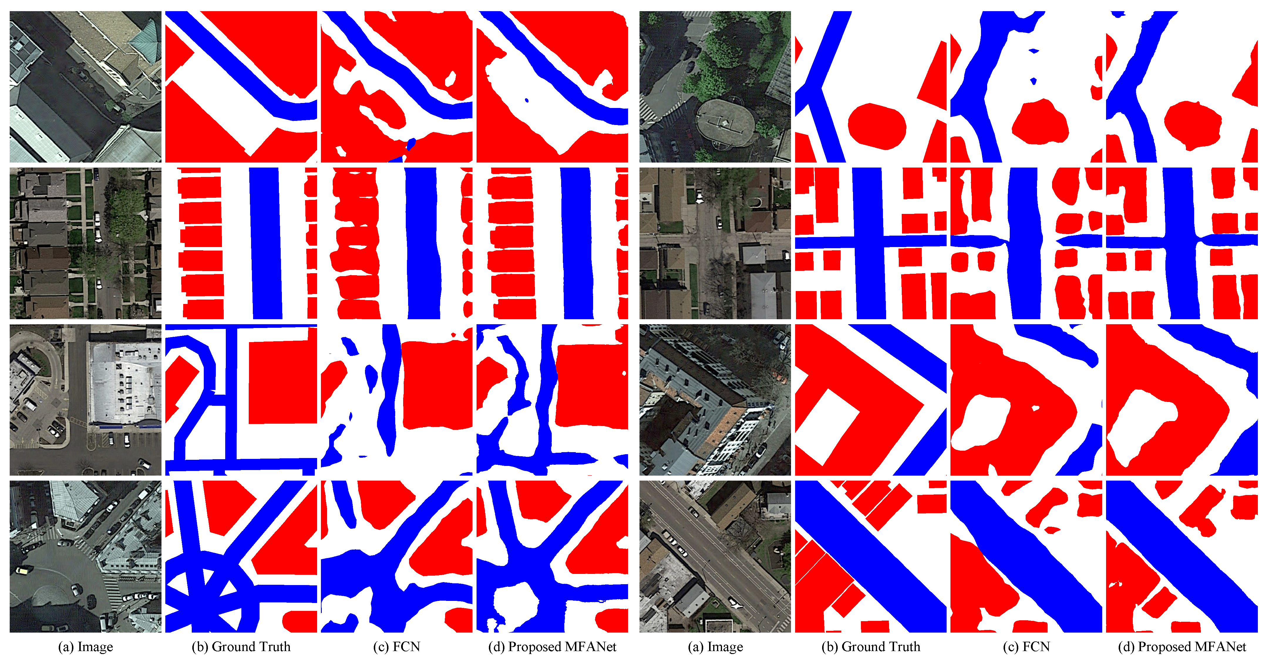
In order to further demonstrate the effectiveness of the proposed MFANet, we also conduct comparative experiments on AISD. The experimental results are shown in Table 8, and MFANet achieves the best performance on the testing set. The visualization results on the testing set are shown in Figure 10. The results in the first row show that MFANet removes distractors, the results in the second row show the fine segmentation for buildings using MFANet, and the results in the third row show the relatively complete prediction for roads compared with baseline network FCN. These results coincide with the prediction results on LandCover dataset. In addition, it is noted that the prediction results shown in the last row are closer to the original images than the ground truths, because the annotation of the dataset is not so fine. These results once again prove the proposed network’s powerful feature extraction capability and high-resolution detail recovery capability for high-resolution remote sensing images.
4. Discussion
Compared with other semantic segmentation methods, our proposed MFANet has three advantages for land cover classification results. First, our network has an advantage in identifying distractors. This is due to the added CFC module enhancing the extraction of deep convolution features by modeling channel interdependence, which alleviates the phenomenon of the same objects with different spectrum and different objects with the same spectrum in remote sensing images to a certain extent. Second, our network may segment more complete targets at the same time, because the used MFAU modules take into account the different representations of features of adjacent stages and global context information to generate a twice-weighted combination of features. This is of great guiding significance for restoring the positioning of high-resolution remote sensing images. Third, the predicted edges of our network are more realistic, because the CLR module added before the last up-sampling gradually reduces the number of channels in two steps to achieve the purpose of refining the restored high-resolution features. In short, the proposed MFANet has a powerful feature extraction capability and a high-resolution detail recovery capability for high-resolution remote sensing images. However, there is still room for further improvement. In the future, we will do further work on recovering high-resolution detailed information.
5. Conclusions
In this work, a new semantic segmentation network MFANet is proposed to solve the land cover classification problem of high-resolution remote sensing images. The MFANet is improved in two aspects: deep feature extraction and up-sampling feature fusion. The proposed CFC module extracts deeper features and filters redundant channel information at the end of a backbone network, which optimizes the learned context. The main idea of the improved MFAU module is to use higher-level features to provide guidance information for low-level features, and high-level features further provide guidance information for newly obtained features, which is of great significance for restoring the positioning of high-resolution remote sensing images. The CLR module is used to gradually refine restored high-resolution feature maps. Experimental results show that the proposed method achieves state-of-the-art performance of 86.45% mean IOU on LandCover dataset.
Author Contributions
Conceptualization, B.C., M.X., and J.H.; methodology, B.C. and M.X.; software, B.C.; validation, B.C. and M.X.; formal analysis, B.C., M.X., and J.H.; investigation, B.C. and M.X.; resources, M.X.; data curation, M.X.; writing–original draft preparation, B.C.; writing–review and editing, M.X.; visualization, B.C.; supervision, M.X.; project administration, M.X.; funding acquisition, M.X. All authors have read and agreed to the published version of the manuscript.
Funding
This research was funded by the National Natural Science Foundation of PR China of grant number 42075130, 61773219.
Data Availability Statement
The data and the code of this study are available from the corresponding author upon request. ([email protected])
Conflicts of Interest
The authors declare no conflict of interest.
References
- Grinias, I.; Panagiotakis, C.; Tziritas, G. MRF-based Segmentation and Unsupervised Classification for Building and Road Detection in Peri-urban Areas of High-resolution. ISPRS J. Photogramm. Remote. Sens. 2016, 122, 145–166. [Google Scholar] [CrossRef]
- Pauleit, S.; Duhme, F. Assessing the environmental performance of land cover types for urban planning. Landsc. Urban Plan. 2000, 52, 1–20. [Google Scholar] [CrossRef]
- Potapov, P.V.; Turubanova, S.; Tyukavina, A.; Krylov, A.; McCarty, J.; Radeloff, V.; Hansen, M. Eastern Europe’s forest cover dynamics from 1985 to 2012 quantified from the full Landsat archive. Remote. Sens. Environ. 2015, 159, 28–43. [Google Scholar] [CrossRef]
- Gerard, F.; Petit, S.; Smith, G.; Thomson, A.; Brown, N.; Manchester, S.; Wadsworth, R.; Bugar, G.; Halada, L.; Bezak, P.; et al. Land cover change in Europe between 1950 and 2000 determined employing aerial photography. Prog. Phys. Geogr. 2010, 34, 183–205. [Google Scholar] [CrossRef] [Green Version]
- Otukei, J.R.; Blaschke, T. Land cover change assessment using decision trees, support vector machines and maximum likelihood classification algorithms. Int. J. Appl. Earth Obs. Geoinf. 2010, 12, S27–S31. [Google Scholar] [CrossRef]
- Foody, G.M.; Mathur, A. A relative evaluation of multiclass image classification by support vector machines. IEEE Trans. Geosci. Remote. Sens. 2004, 42, 1335–1343. [Google Scholar] [CrossRef] [Green Version]
- Mas, J.F.; Flores, J.J. The application of artificial neural networks to the analysis of remotely sensed data. Int. J. Remote. Sens. 2008, 29, 617–663. [Google Scholar] [CrossRef]
- Friedl, M.A.; Brodley, C.E. Decision tree classification of land cover from remotely sensed data. Remote. Sens. Environ. 1997, 61, 399–409. [Google Scholar] [CrossRef]
- Atzberger, C. Advances in remote sensing of agriculture: Context description, existing operational monitoring systems and major information needs. Remote. Sens. 2013, 5, 949–981. [Google Scholar] [CrossRef] [Green Version]
- Boguszewski, A.; Batorski, D.; Ziemba-Jankowska, N.; Zambrzycka, A.; Dziedzic, T. LandCover. ai: Dataset for Automatic Mapping of Buildings, Woodlands and Water from Aerial Imagery. arXiv 2020, arXiv:2005.02264. [Google Scholar]
- Long, J.; Shelhamer, E.; Darrell, T. Fully convolutional networks for semantic segmentation. In Proceedings of the IEEE Conference on Computer Vision and Pattern Recognition, Boston, MA, USA, 7–12 June 2015; pp. 3431–3440. [Google Scholar]
- Ronneberger, O.; Fischer, P.; Brox, T. U-net: Convolutional networks for biomedical image segmentation. In International Conference On Medical Image Computing And Computer-Assisted Intervention; Springer: Berlin/Heidelberg, Germany, 2015; pp. 234–241. [Google Scholar]
- Zhao, H.; Shi, J.; Qi, X.; Wang, X.; Jia, J. Pyramid scene parsing network. In Proceedings of the IEEE Conference on Computer Vision and Pattern Recognition, Honolulu, HI, USA, 21–26 July 2017; pp. 2881–2890. [Google Scholar]
- Chen, L.C.; Papandreou, G.; Schroff, F.; Adam, H. Rethinking atrous convolution for semantic image segmentation. arXiv 2017, arXiv:1706.05587. [Google Scholar]
- Yu, C.; Wang, J.; Peng, C.; Gao, C.; Yu, G.; Sang, N. Learning a discriminative feature network for semantic segmentation. In Proceedings of the IEEE Conference on Computer Vision and Pattern Recognition, Salt Lake City, UT, USA, 18–23 June 2018; pp. 1857–1866. [Google Scholar]
- Huan, E.Y.; Wen, G.H. Multilevel and multiscale feature aggregation in deep networks for facial constitution classification. Comput. Math. Methods Med. 2019, 2019, 1258782. [Google Scholar] [CrossRef] [PubMed]
- Chu, Y.; Yang, X.; Li, H.; Ai, D.; Ding, Y.; Fan, J.; Song, H.; Yang, J. Multi-level feature aggregation network for instrument identification of endoscopic images. Phys. Med. Biol. 2020, 65, 165004. [Google Scholar] [CrossRef]
- Fu, J.; Liu, J.; Wang, Y.; Zhou, J.; Wang, C.; Lu, H. Stacked deconvolutional network for semantic segmentation. IEEE Trans. Image Process. 2019, 1. [Google Scholar] [CrossRef] [PubMed]
- Qian, J.; Xia, M.; Zhang, Y.; Liu, J.; Xu, Y. TCDNet: Trilateral Change Detection Network for Google Earth Image. Remote. Sens. 2020, 12, 2669. [Google Scholar] [CrossRef]
- Liu, W.; Rabinovich, A.; Berg, A.C. Parsenet: Looking wider to see better. arXiv 2015, arXiv:1506.04579. [Google Scholar]
- Chen, L.C.; Papandreou, G.; Kokkinos, I.; Murphy, K.; Yuille, A.L. Deeplab: Semantic image segmentation with deep convolutional nets, atrous convolution, and fully connected crfs. IEEE Trans. Pattern Anal. Mach. Intell. 2017, 40, 834–848. [Google Scholar] [CrossRef] [PubMed]
- Badrinarayanan, V.; Kendall, A.; Cipolla, R. Segnet: A deep convolutional encoder-decoder architecture for image segmentation. IEEE Trans. Pattern Anal. Mach. Intell. 2017, 39, 2481–2495. [Google Scholar] [CrossRef]
- Lin, G.; Milan, A.; Shen, C.; Reid, I. Refinenet: Multi-path refinement networks for high-resolution semantic segmentation. In Proceedings of the IEEE Conference on Computer Vision and Pattern Recognition, Honolulu, HI, USA, 21–26 July 2017; pp. 1925–1934. [Google Scholar]
- Chen, L.C.; Zhu, Y.; Papandreou, G.; Schroff, F.; Adam, H. Encoder-decoder with atrous separable convolution for semantic image segmentation. In Proceedings of the European conference on computer vision (ECCV), Munich, Germany, 8–14 September 2018; pp. 801–818. [Google Scholar]
- Saxena, S.; Verbeek, J. Convolutional neural fabrics. Adv. Neural Inf. Process. Syst. 2016, 29, 4053–4061. [Google Scholar]
- Sun, K.; Xiao, B.; Liu, D.; Wang, J. Deep high-resolution representation learning for human pose estimation. In Proceedings of the IEEE Conference on Computer Vision and Pattern Recognition, Long Beach, CA, USA, 15–20 June 2019; pp. 5693–5703. [Google Scholar]
- Yang, M.; Yu, K.; Zhang, C.; Li, Z.; Yang, K. Denseaspp for semantic segmentation in street scenes. In Proceedings of the IEEE Conference on Computer Vision and Pattern Recognition, Salt Lake City, UT, USA, 18–23 June 2018; pp. 3684–3692. [Google Scholar]
- Hu, J.; Shen, L.; Sun, G.; Albanie, S. Squeeze-and-Excitation Networks. IEEE Trans. Pattern Anal. Mach. Intell. 2017, 99, 7132–7141. [Google Scholar]
- Li, H.; Xiong, P.; An, J.; Wang, L. Pyramid attention network for semantic segmentation. arXiv 2018, arXiv:1805.10180. [Google Scholar]
- He, K.; Zhang, X.; Ren, S.; Sun, J. Deep residual learning for image recognition. In Proceedings of the IEEE Conference on Computer Vision and Pattern Recognition, Las Vegas, Nevada, USA, 26 June – 1 July 2016; pp. 770–778. [Google Scholar]
- Ni, Z.L.; Bian, G.B.; Wang, G.A.; Zhou, X.H.; Hou, Z.G.; Chen, H.B.; Xie, X.L. Pyramid attention aggregation network for semantic segmentation of surgical instruments. In Proceedings of the AAAI Conference on Artificial Intelligence, Hilton Midtown, New York, USA, 7–12 February 2020; Volume 34, pp. 11782–11790. [Google Scholar]
- Ni, Z.L.; Bian, G.B.; Hou, Z.G.; Zhou, X.H.; Xie, X.L.; Li, Z. Attention-guided lightweight network for real-time segmentation of robotic surgical instruments. In Proceedings of the 2020 IEEE International Conference on Robotics and Automation (ICRA), Paris, France, 17–21 May 2020; pp. 9939–9945. [Google Scholar]
- Xia, M.; Wang, K.; Song, W.; Chen, C.; Li, Y. Non-intrusive load disaggregation based on composite deep long short-term memory network. Expert Syst. Appl. 2020, 160, 113669. [Google Scholar] [CrossRef]
- Xia, M.; Wang, T.; Zhang, Y.; Liu, J.; Xu, Y. Cloud/shadow segmentation based on global attention feature fusion residual network for remote sensing imagery. Int. J. Remote. Sens. 2021, 42, 2022–2045. [Google Scholar] [CrossRef]
- Sandler, M.; Howard, A.; Zhu, M.; Zhmoginov, A.; Chen, L.C. Mobilenetv2: Inverted residuals and linear bottlenecks. In Proceedings of the IEEE Conference on Computer Vision and Pattern Recognition, Salt Lake City, UT, USA, 18–23 June 2018; pp. 4510–4520. [Google Scholar]
- Xia, M.; Zhang, X.; Weng, L.; Xu, Y. Multi-Stage Feature Constraints Learning for Age Estimation. IEEE Trans. Inf. Forensics Secur. 2020, 15, 2417–2428. [Google Scholar] [CrossRef]
- He, K.; Zhang, X.; Ren, S.; Sun, J. Identity mappings in deep residual networks. In Proceedings of the European Conference on Computer Vision, Amsterdam, Netherlands, 11–14 October 2016; pp. 630–645. [Google Scholar]
- Kaiser, P.; Wegner, J.D.; Lucchi, A.; Jaggi, M.; Hofmann, T.; Schindler, K. Learning aerial image segmentation from online maps. IEEE Trans. Geosci. Remote. Sens. 2017, 55, 6054–6068. [Google Scholar] [CrossRef]
- Chen, L.C.; Papandreou, G.; Kokkinos, I.; Murphy, K.; Yuille, A.L. Semantic image segmentation with deep convolutional nets and fully connected crfs. arXiv 2014, arXiv:1412.7062. [Google Scholar]
- Xia, M.; Tian, N.; Zhang, Y.; Xu, Y.; Zhang, X. Dilated multi-scale cascade forest for satellite image classification. Int. J. Remote. Sens. 2020, 41, 7779–7800. [Google Scholar] [CrossRef]
- Xia, M.; Cui, Y.; Zhang, Y.; Liu, J.; Xu, Y. DAU-Net: A Novel Water Areas Segmentation Structure for Remote Sensing Image. Int. J. Remote. Sens. 2021, 42, 2594–2621. [Google Scholar] [CrossRef]
- Li, H.; Xiong, P.; Fan, H.; Sun, J. Dfanet: Deep feature aggregation for real-time semantic segmentation. In Proceedings of the IEEE Conference on Computer Vision and Pattern Recognition, Long Beach, CA, USA, 15–20 June 2019; pp. 9522–9531. [Google Scholar]
- Fu, J.; Liu, J.; Tian, H.; Li, Y.; Bao, Y.; Fang, Z.; Lu, H. Dual attention network for scene segmentation. In Proceedings of the IEEE Conference on Computer Vision and Pattern Recognition, Long Beach, California, USA, 15–20 June 2019; pp. 3146–3154. [Google Scholar]
- Mehta, S.; Rastegari, M.; Shapiro, L.; Hajishirzi, H. Espnetv2: A light-weight, power efficient, and general purpose convolutional neural network. In Proceedings of the IEEE Conference on Computer Vision and Pattern Recognition, Long Beach, CA, USA, 15–20 June 2019; pp. 9190–9200. [Google Scholar]
- Zhao, H.; Qi, X.; Shen, X.; Shi, J.; Jia, J. Icnet for real-time semantic segmentation on high-resolution images. In Proceedings of the European Conference on Computer Vision (ECCV), Munich, Germany, 8–14 September 2018; pp. 405–420. [Google Scholar]
- Wu, T.; Tang, S.; Zhang, R.; Zhang, Y. Cgnet: A light-weight context guided network for semantic segmentation. arXiv 2018, arXiv:1811.08201. [Google Scholar]
- Wang, J.; Sun, K.; Cheng, T.; Jiang, B.; Deng, C.; Zhao, Y.; Liu, D.; Mu, Y.; Tan, M.; Wang, X. Deep high-resolution representation learning for visual recognition. IEEE Trans. Pattern Anal. Mach. Intell. 2020, 9, 1. [Google Scholar] [CrossRef] [PubMed] [Green Version]
- Yu, C.; Wang, J.; Peng, C.; Gao, C.; Yu, G.; Sang, N. Bisenet: Bilateral segmentation network for real-time semantic segmentation. In Proceedings of the European Conference on Computer Vision (ECCV), Munich, Germany, 8–14 September 2018; pp. 325–341. [Google Scholar]
Figure 1.
The architecture of Multi-level Feature Aggregation Network (MFANet). The modified ResNet-50 is used to extract features of different levels. Then the deep semantic features are further extracted by Channel Feature Compression (CFC), the feature fusion and location recovery are completed by Multi-level Feature Attention Upsample (MFAU), and the recovered high-resolution details are further refined by Channel Ladder Refinement (CLR). The blue and red lines represent down sampling and up sampling operations respectively.

Figure 2.
The structure of Channel Feature Compression module. ‘GAP’ represents the global average pooling operation. ‘r’ is the reduction ratio. ‘ H×W×C’ represents the shape of the features.
Figure 2.
The structure of Channel Feature Compression module. ‘GAP’ represents the global average pooling operation. ‘r’ is the reduction ratio. ‘ H×W×C’ represents the shape of the features.

Figure 3.
The structure of Multi-level Feature Attention Upsample module.

Figure 4.
The structure of Channel Ladder Refinement module. ‘’ denotes ‘BN - ReLU -Conv’ is repeated twice.
Figure 4.
The structure of Channel Ladder Refinement module. ‘’ denotes ‘BN - ReLU -Conv’ is repeated twice.

Figure 5.
An example for LandCover dataset. (a) The original image; (b) Manually annotated label. The parts shown by the dotted line belong to the background class while they are easy to be misclassified. The objects circled by the solid line are the target classes while they are easy to recognize as background.

Figure 6.
Prediction results of images with two classifications. (a) The original images; (b) Corresponding labels; (c) The predicted maps of FCN, (d) The predicted maps of DeepLabv3+; (e) The predicted maps ofBiSeNet; (f) The predicted maps of DenseASPP; (g) The predicted maps of proposed MFANet.
Figure 6.
Prediction results of images with two classifications. (a) The original images; (b) Corresponding labels; (c) The predicted maps of FCN, (d) The predicted maps of DeepLabv3+; (e) The predicted maps ofBiSeNet; (f) The predicted maps of DenseASPP; (g) The predicted maps of proposed MFANet.

Figure 7.
Prediction results of images with three classifications.(a) The original images; (b) Corresponding labels; (c) The predicted maps of FCN; (d) The predicted maps of DeepLabv3+; (e) The predicted maps of BiSeNet; (f) The predicted maps of DenseASPP; (g) The predicted maps of proposed MFANet.

Figure 8.
Prediction results of images with four classifications. (a) The original images; (b) Corresponding labels; (c) The predicted maps of FCN; (d) The predicted maps of DeepLabv3+; (e) The predicted maps of BiSeNet; (f) The predicted maps of DenseASPP; (g) The predicted maps of proposed MFANet.

Figure 9.
Results of MFANet on LandCover testing set. (a) The original images; (b) Corresponding labels; (c) The predicted maps of proposed MFANet.
Figure 9.
Results of MFANet on LandCover testing set. (a) The original images; (b) Corresponding labels; (c) The predicted maps of proposed MFANet.

Figure 10.
Results of MFANet on AISD testing set. (a) The original images; (b) Corresponding labels; (c) The predicted maps of FCN; (d) The predicted maps of proposed MFANet.
Figure 10.
Results of MFANet on AISD testing set. (a) The original images; (b) Corresponding labels; (c) The predicted maps of FCN; (d) The predicted maps of proposed MFANet.


Table 1.
An explanation of five Blocks from the extraction network ResNet-50 . Note that the stride of Block-5 is reset to 1.
Table 1.
An explanation of five Blocks from the extraction network ResNet-50 . Note that the stride of Block-5 is reset to 1.
| Layer name | Output size | 50-layer |
|---|---|---|
| Block-1 | ||
| Block-2 | ||
| Block-3 | ||
| Block-4 | ||
| Block-5 |
Table 2.
It is important to set the appropriate reduction ratio in the Channel Feature Compression (CFC) (bold represents the best result).
Table 2.
It is important to set the appropriate reduction ratio in the Channel Feature Compression (CFC) (bold represents the best result).
| Reduction Ratio r | mIoU(%) | mPA(%) | Parameter(M) | Parameter(G) |
|---|---|---|---|---|
| 2 | 84.80 | 90.78 | 36.149 | 42.833 |
| 4 | 84.93 | 90.91 | 34.575 | 42.832 |
| 8 | 84.71 | 90.56 | 33.788 | 42.831 |
| 16 | 84.75 | 90.61 | 33.395 | 42.830 |
Table 3.
The performance comparison of the networks using the proposed modules in turn. ‘ResNet50-Baseline’ means the segmentation network with three types of modules: SE, GAU, and RRB, and it uses ResNet50 as the backbone. ‘CFC’ means using CFC module to replace the SE module. ‘MFAU’ means using MFAU module to replace the GAU module. ‘CLR’ means using CLR module to replace the RRB module (bold represents the best result).
| Method | mIoU(%) | mPA(%) | Parameter(M) | Parameter(G) |
|---|---|---|---|---|
| ResNet50-Baseline | 84.57 | 89.82 | 35.090 | 44.478 |
| ResNet50+CFC | 84.93 | 90.91 | 34.575 | 42.832 |
| ResNet50+MFAU | 85.66 | 91.37 | 39.431 | 82.398 |
| ResNet50+CLR | 84.93 | 91.10 | 34.580 | 42.837 |
| ResNet50+CFC+MFAU+CLR(MFANet) | 86.45 | 92.09 | 38.969 | 84.161 |
Table 4.
It is important to set the appropriate buffer factor in Channel Ladder Refinement (CLR) (bold represents the best result).
Table 4.
It is important to set the appropriate buffer factor in Channel Ladder Refinement (CLR) (bold represents the best result).
| Buffer Factor b | mIoU(%) | mPA(%) | Parameter(M) | Parameter(G) |
|---|---|---|---|---|
| 1 | 84.78 | 90.72 | 35.097 | 44.982 |
| 4 | 84.84 | 90.78 | 35.102 | 44.987 |
| 9 | 84.67 | 90.71 | 35.123 | 45.007 |
| 16 | 84.93 | 91.10 | 35.175 | 45.061 |
Table 5.
Influence of using different ratio combinations for the three convolutions of the Conv-5 block from ResNet-50 on algorithm performance (bold represents the best result).
Table 5.
Influence of using different ratio combinations for the three convolutions of the Conv-5 block from ResNet-50 on algorithm performance (bold represents the best result).
| Dilation Ratios | mIoU(%) | PA(%) | mPA(%) |
|---|---|---|---|
| 1-1-1 | 86.44 | 95.00 | 92.39 |
| 1-2-3 | 86.32 | 94.64 | 92.24 |
| 2-2-2 | 86.40 | 94.68 | 91.97 |
| 1-2-5 | 86.32 | 94.64 | 92.09 |
Table 6.
Results on LandCover testing set. Methods pre-trained are marked with ‘†’ (bold represents the best result).
Table 6.
Results on LandCover testing set. Methods pre-trained are marked with ‘†’ (bold represents the best result).
| Method | Parameters(M) | FLOP(G) | MPA(%) | fwIoU(%) | mIoU(%) |
|---|---|---|---|---|---|
| DFANet [42] | 2.024 | 0.913 | 76.96 | 81.27 | 68.52 |
| SegNet [22] | 29.445 | 178.342 | 77.19 | 81.78 | 71.85 |
| DANet [43] | 49.612 | 206.121 | 83.75 | 85.36 | 75.2 |
| ESPNetv2 [44] | 2.159 | 0.754 | 84.72 | 86.28 | 77.67 |
| ICNet [45] | 28.293 | 10.087 | 85.04 | 86.03 | 78.82 |
| CGNet [46] | 0.492 | 3.37 | 88.74 | 87.38 | 80.96 |
| HRNet [47] | 1.537 | 5.074 | 88.03 | 87.03 | 81.27 |
| Ours-MobileNetv2 | 2.156 | 8.601 | 88.97 | 87.55 | 81.53 |
| PSPNet [13] | 48.757 | 184.128 | 87.87 | 88.68 | 82.37 |
| U-Net [12] | 17.268 | 177.805 | 87.96 | 87.66 | 82.52 |
| Ours- ResNet50 | 38.969 | 84.161 | 89.63 | 88.73 | 82.78 |
| FCN-16s [11] | 15.318 | 89.261 | 89.54 | 89.12 | 82.71 |
| DeeplabV3+ [24] | 54.701 | 82.665 | 90.39 | 88.95 | 84.17 |
| BiSeNet [48] | 12.796 | 12.963 | 90.42 | 89.1 | 84.45 |
| DenseASPP [27] | 10.201 | 48.677 | 91.35 | 89.35 | 85.04 |
| Ours- MobileNetv2 | 2.156 | 8.601 | 91.4 | 89.45 | 85.49 |
| Ours-ResNet50 | 38.969 | 84.161 | 92.09 | 89.89 | 86.45 |
Table 7.
Per-class results on LandCover testing set. Methods that are pre-trained are marked with ‘†’ (bold represents the best result).
Table 7.
Per-class results on LandCover testing set. Methods that are pre-trained are marked with ‘†’ (bold represents the best result).
| Class | Buildings | Woodlands | Water | Backgroud | Overall |
|---|---|---|---|---|---|
| FCN-16s | 62.59 | 87.15 | 90.46 | 90.64 | 82.71 |
| DeeplabV3+ | 68.95 | 86.67 | 90.51 | 90.53 | 84.17 |
| BiSeNet | 69.41 | 86.87 | 90.87 | 90.63 | 84.45 |
| DenseASPP | 72.03 | 87.14 | 90.05 | 90.93 | 85.04 |
| Ours-MobileNetv2 | 72.78 | 87.36 | 90.94 | 90.86 | 85.49 |
| Ours-ResNet | 75.09 | 87.78 | 91.66 | 91.25 | 86.45 |
Table 8.
Results on aerial image segmentation dataset (AISD) testing set (bold represents the best result).
Table 8.
Results on aerial image segmentation dataset (AISD) testing set (bold represents the best result).
| Method | MPA(%) | fwIoU(%) | mIoU(%) |
|---|---|---|---|
| FCN-16s | 83.22 | 71.96 | 71.78 |
| U-Net | 84.03 | 73.16 | 72.89 |
| BiSeNet | 84.88 | 74.18 | 74.05 |
| MFANet | 85.89 | 75.67 | 75.61 |
Publisher’s Note: MDPI stays neutral with regard to jurisdictional claims in published maps and institutional affiliations. |
© 2021 by the authors. Licensee MDPI, Basel, Switzerland. This article is an open access article distributed under the terms and conditions of the Creative Commons Attribution (CC BY) license (http://creativecommons.org/licenses/by/4.0/).
Share and Cite
MDPI and ACS Style
Chen, B.; Xia, M.; Huang, J. MFANet: A Multi-Level Feature Aggregation Network for Semantic Segmentation of Land Cover. Remote Sens. 2021, 13, 731. https://0-doi-org.brum.beds.ac.uk/10.3390/rs13040731
AMA Style
Chen B, Xia M, Huang J. MFANet: A Multi-Level Feature Aggregation Network for Semantic Segmentation of Land Cover. Remote Sensing. 2021; 13(4):731. https://0-doi-org.brum.beds.ac.uk/10.3390/rs13040731
Chicago/Turabian StyleChen, Bingyu, Min Xia, and Junqing Huang. 2021. "MFANet: A Multi-Level Feature Aggregation Network for Semantic Segmentation of Land Cover" Remote Sensing 13, no. 4: 731. https://0-doi-org.brum.beds.ac.uk/10.3390/rs13040731
Note that from the first issue of 2016, this journal uses article numbers instead of page numbers. See further details here.