1. Introduction
Autonomous navigation for agricultural robots is essential for promoting the automation of modern agriculture, especially in ways to reduce labor intensity and enhance operation efficiency [
1,
2]. As a branch of autonomous navigation, visual navigation has developed rapidly in recent years, due to the improvements of computer calculation speed and visual sensors [
3]. The most important issue of visual navigation primarily concerns extracting a guidance path according to the environment. When the drainage, light, and field management in the process of rice cultivation taken into account, rice is usually planted in rows, especially when transplanted by machines. Therefore, many researchers have tried extracting the guidance path for unmanned agricultural machinery utilizing this feature.
Typically, most of the methods proposed for crop row detection in recent years share the same architecture consisting of four steps, which are image grayscale transformation, image binarization, feature point extraction, and crop row identification. The excess green
Excess green graying method, which was reported to yield good results by Woebbecke et al. [
4], is the most widely used grayscale transformation method due to its excellent performance in distinguishing green plants and background under a wide range of illumination conditions. Once the grayscale transformation is completed, the Otsu method [
5], a kind of nonparametric and unsupervised method of automatic threshold selection for image binarization, can be applied. The principle of the Otsu method is to select an optimal threshold by the discriminant criterion, thereby maximizing the separability of the resultant classes in gray levels. As for feature point extraction, the horizontal strip method combined with the vertical projection method serves as the most common solution. Søgaard and Olsen [
6] divided a grayscale image into 15 horizontal strips, and then computed the vertical sum of gray values in each strip, with the maximum denoting the center of crop row in each strip. Lastly, crop rows are detected by the center points. On the basis of horizontal strips, Sainz-Costa et al. [
7] developed a strategy for identifying crop rows through the analysis of video sequences. Hough transformation [
8] is one of the most commonly used machine vision methods for identifying crop rows [
9]. Least squares fitting has become another commonly used method to identify crop rows since the separation of weeds and crops has improved. Billingsley and Schoenfisch [
10] used least squares fitting on the basis of information from three row segments to detect crop row guidance information. This image processing architecture attached with these classical methods makes it possible to detect crop rows, especially in some simple and specific circumstances.
Various studies on crop rows detection focused on making improvements in some steps of this general architecture. To further distinguish crops and weeds after the binarization using the typical Otsu method, Montalvo et al. [
11] designed a method called double thresholding. Considering the crop row arrangement is known in the field, as well as the extrinsic and intrinsic camera system parameters, Guerrero et al. [
12] proposed an expert system based on the geometry, and a correction was applied through the well-tested and robust Theil–Sen estimator in order to adjust the detected lines to the real ones. Guoquan Jiang et al. [
13] constructed a multi-region of interest method, which integrates the features of multiple rows according to a geometry constraint. In order to enhance the robustness of crop row detection, García et al. [
14] divided crop row identification into three steps: extraction of candidate points from reference lines, regression analysis for fitting polynomial equations, and final crop row selection. The method could deal with uncontrolled lighting conditions and unexpected gaps in crop rows. Many scholars have applied crop row detection algorithms to visual navigation systems and conducted field experiments. Guerrero et al. [
15] designed a computer vision system involving two modules. The first module aimed to estimate the crop rows as accurately as possible, while the second module used the crop rows to control the tractor guidance and the overlapping. Basso et al. [
16] proposed a crop row detection algorithm featuring Hough transform of an embedded guiding system for unmanned aerial vehicle (UAV). Tenhunen et al. [
17] proposed a method for recognition of plantlet rows by means of pattern recognition. Li et al. [
18] designed a pipeline-friendly crop row detection system using field programmable gate array (FPGA) architecture to reduce the resource utilization and balance the utilization of different onboard resources. Rabab et al. [
19] proposed an efficient crop row detection algorithm which functions without the use of templates and most other prior information. The studies mentioned above mainly focused on crop row detection and visual navigation in dry fields.
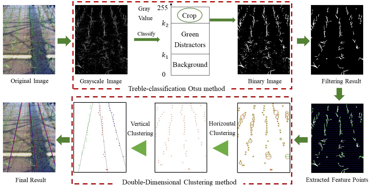
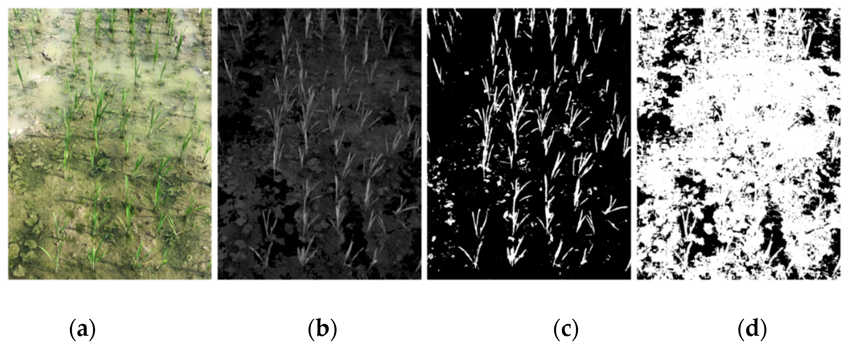
However, it is difficult to achieve satisfying results of image segmentation in some complex agricultural environments, especially in paddy fields. A paddy field is a kind of open and complex environment, often accompanied by weed and duckweed, especially in areas without proper management. Some typical images in paddy fields are shown in
Figure 1. Weed and duckweed are floating on the water, showing a green color similar to the color of the rice seedings. In addition, after fertilizing the paddy field, eutrophication often occurs, which can also cause the water surface to appear with a color similar to the color of the rice seedings. These are the reasons for the significantly increased difficulty in distinguishing crops from background. In this case, the typical Otsu method tends to bring a lot of noise, which totally disturbs the subsequent extraction of the crop row lines. Thus, the traditional architecture of crop row detection does not function well in paddy fields, attributed to the undesirable results of image binarization. Several studies were devoted to identifying crop rows without image segmentation. Aiming at a visual navigation algorithm for a paddy field weeding robot, Zhang et al. [
3] applied the smallest univalue segment assimilating nucleus (SUSAN) corner detection method directly after obtaining the grayscale image without image binarization. This strategy cleverly bypasses the problem of segmentation for paddy field images, but it increases the extent of time-consuming calculation.
In addition to the general architecture, stereo vision and neural networks have also been tested to detect the crop rows when the heights of the weeds and crop plants above ground are highly visible and when the weeds and crop plants differ in height [
20]. Kise and Zhang [
21] developed a stereo-vision-based crop-row tracking navigation system for agricultural machinery. Zhai et al. [
1] developed a multi-crop-row detection algorithm to locate the three-dimensional (3D) position of crop rows according to their spatial distribution. Fue et al. [
22] utilized stereo vision to determine 3D boll location and row detection, and the performance of this method showed promise as a method to assist with the real-time kinematic global navigation satellite system (RTK-GNSS) navigation. Adhikari et al. [
23] trained a deep convolutional encoder decoder network to detect crop lines using semantic graphics. Ponnambalam et al. [
24] designed a convolution neural network to segment input images based on red, green and blue color system (RGB) into crop and non-crop regions. Although these approaches achieved good results, there is still no superiority of stereo vision and deep learning over traditional architecture in terms of time consumption, and this will cause a significant burden for computation devices. Therefore, there is still a long way to go for the industrialization of crop row detection using stereo vision and neural network.
Although the abovementioned algorithms were proposed for crop row detection, the technical issue of image binarization of paddy fields still remains, which leads to the dilemma that traditional crop row detection methods based on image segmentation may fail to work in a paddy field environment. All these factors demonstrate that the crop row detection method of paddy fields should be originally designed in order to minimize the disturbance caused by the paddy field environment. Guijarro et al. [
25] proved that distinguishing objects with different color characteristics by image segmentation is feasible. Thus, in this paper, to reduce the disturbance caused by weed and duckweed, the treble-classification Otsu method and double-dimensional clustering method for paddy fields are proposed, which improve the robustness of separating crop rows from complex paddy fields. The method proposed in this paper is improved on the basis of previous work, such as the typical Otsu method and clustering method. The purpose of this work is to meet the needs of low-price, lightweight computing and real-time performance of the unmanned system in paddy fields. The establishment of a flexible and reliable unmanned system is of great significance for the realization of large-scale paddy field intelligent unmanned management.
2. Materials and Methods
The method proposed in this paper mainly comprises three modules: image segmentation, feature point extraction, and crop row detection, as described below.
2.1. Image Segmentation
2.1.1. Grayscale Transformation
The original chromatic image contains a large amount of information, the effective part of which is only the location of the green plant. This means that directly processing chromatic images will lead to unnecessary calculations due to information redundancy. To emphasize the living plant tissue, which is the basis of the subsequent steps, and weaken the rest of image [
13], existing information needs dimensionality reduction processing. Thus, once the images are captured in the RGB color format, the first step is grayscale transformation.
Color is one of the most common indices used to discriminate plants from background clutter in computer vision [
26]. A pixel where the predominant spectral component is the green is considered vegetation [
12]. Through this strategy, color index-based approaches are resorted to achieve grayscale transformation. Generally, common green indices methods include normalized difference index (NDI) [
27], excess green index (ExG) [
4], color index of vegetation extraction (CIVE) [
28], and vegetative index (VEG) [
29].
The original images are obtained from the paddy field. Because of the water situation, it is necessary to take into account the reflections that frequently appear on the water surface. When only the intensity of the light source changes, the components of the light reflected on the surface of the same material are the same. Hence, the following formula is defined:
where
is the reflection intensity of the water surface under strong light,
is the reflection intensity of the water surface without strong light reflection, and
is a constant greater than 1.
For the same water surface, the reflective components under strong light reflection and the reflective components without strong light reflection are the same, where only the intensity differs. Thus, for each RGB color channel, the following formula is defined:
where
, and
are the changes in the RGB channels due to changes in light intensity, respectively.
,
, and
are the values of RGB channels without strong light reflection, respectively.
This means that if the values of color channels can be expressed in the form of rates, the green index will not be bothered by the intensity of light. Under the same light source conditions, the reflection intensity of the water surface in the paddy field is much greater than that in the upland field. Although the above methods are all equipped with robustness to various lighting conditions,
CIVE and
VEG will fluctuate within a certain range as the reflected light intensity changes because the channel values of RGB cannot be expressed in the form of rates [
13,
30]. Therefore, the two methods of
CIVE and
VEG were eliminated from the candidate list. Additionally, the result of
NDI is a near-binary image [
26] with little capability to cope with the separation of weed and duckweed from rice seedings. Therefore, after comparing the above green indices, the
ExG index was selected to process the images of paddy fields.
2.1.2. Thresholding with Treble-Classification Otsu Method
After the grayscale transformation is completed, large amounts of invalid information still remain in the image, while only the green plant tissues need to be considered. In addition to multi-channel color information, it is also necessary to refine the grayscale information. Therefore, image binarization, which means to reduce a multi-value digital signal into a two-value binary signal [
31], is the second step of image segmentation. The Otsu method [
5] is one of the best thresholding techniques for image binarization. The basic idea of the Otsu method is to dichotomize the pixels into two classes (background and objects) using a selected optimal threshold. This binarization method has been proven to be adaptively effective in different studies related to image segmentation between crop and background [
32,
33]. However, the dichotomy between objects and background is too rough to distinguish the real crops and green distractors, which will be both identified as objects in a binary image, especially in complex conditions such as paddy fields.
For the paddy field environment, the existence of green distractors can be explained as weed, duckweed, and cyanobacteria [
3]. Furthermore, the water in the paddy field undergoes eutrophication after fertilization, resulting in a green paddy field environment. According to the above issues, the typical Otsu method needs to be improved in order to deal with the separation of real rice seedings and green distractors, rather than simply classify them as objects. To further classify the objects which include both rice seedings and green distractors, the typical Otsu method based on dichotomy was improved to be based on the trichotomy.
The pixels of a given greyscale image can be represented in
gray levels
. The number of pixels at level
is denoted by
, and the total number of pixels is denoted by
. To simplify the discussion, the gray-level histogram is normalized and regarded as a probability distribution [
5].
Now, suppose that two thresholds
are selected, which divides the pixels into three classes
,
, and
(background, green distractor, and crop).
denotes pixels with levels
,
denotes pixels with levels
, and
denotes pixels with levels
. Then, the probabilities of class occurrence and the class mean levels, respectively, are given by
According to the Bayes theorem, the mean levels of the pixels assigned to classes are given by
where the total mean level of the grayscale image is
The following relationships can be easily verified for any combination of
:
where
is the total mean level of the greyscale image, defined as
Referring to the evaluation of “goodness” of the threshold at a selected level in the Otsu method, the discriminant criterion is introduced.
where
is the total variance, defined as
and
is the between-class variance, defined as
Considering that the total variance
is a constant once the image is defined, the only way to maximize
is to maximize
. Equation (18) can be converted into the following form using Equations (14) and (15):
Thus, the issue of maximizing discriminant criterion
is reduced to an optimization problem to search for a combination of
and
that maximizes between-class variance
. The optimal threshold combination of
and
is
The processing steps of the treble-classification Otsu method are as follows:
Calculate the normalized histogram of the input greyscale image, and record the minimum gray value and the maximum gray value as and .
Traverse from to , and calculate and .
Traverse from to , and calculate and .
Traverse from to , then traverse from to , and calculate , , and .
Record , which maximize . If the combination of is not unique, calculate the mean value of .
2.1.3. Filtering Operations
Generally, the initial binary image obtained using the thresholding method does not clearly represent the original information of the crop row. Some noise pixels are distributed among the crop rows in the form of islands, leading to interference with crop row detection. Although subsequent algorithms are not sensitive to the noise pixels of small island shapes, it is a wise choice to remove as much noise as possible that may cause interference. According to the theory in this research, all of the white pixels should represent the position of the crops, rather than the islands of noise. Therefore, to remove the small, discrete, and insignificant white patches, an extra filtering process is applied after image binarization. In this paper, isolated connected domains are traversed, and those with an area less than 30 pixels should be eliminated.
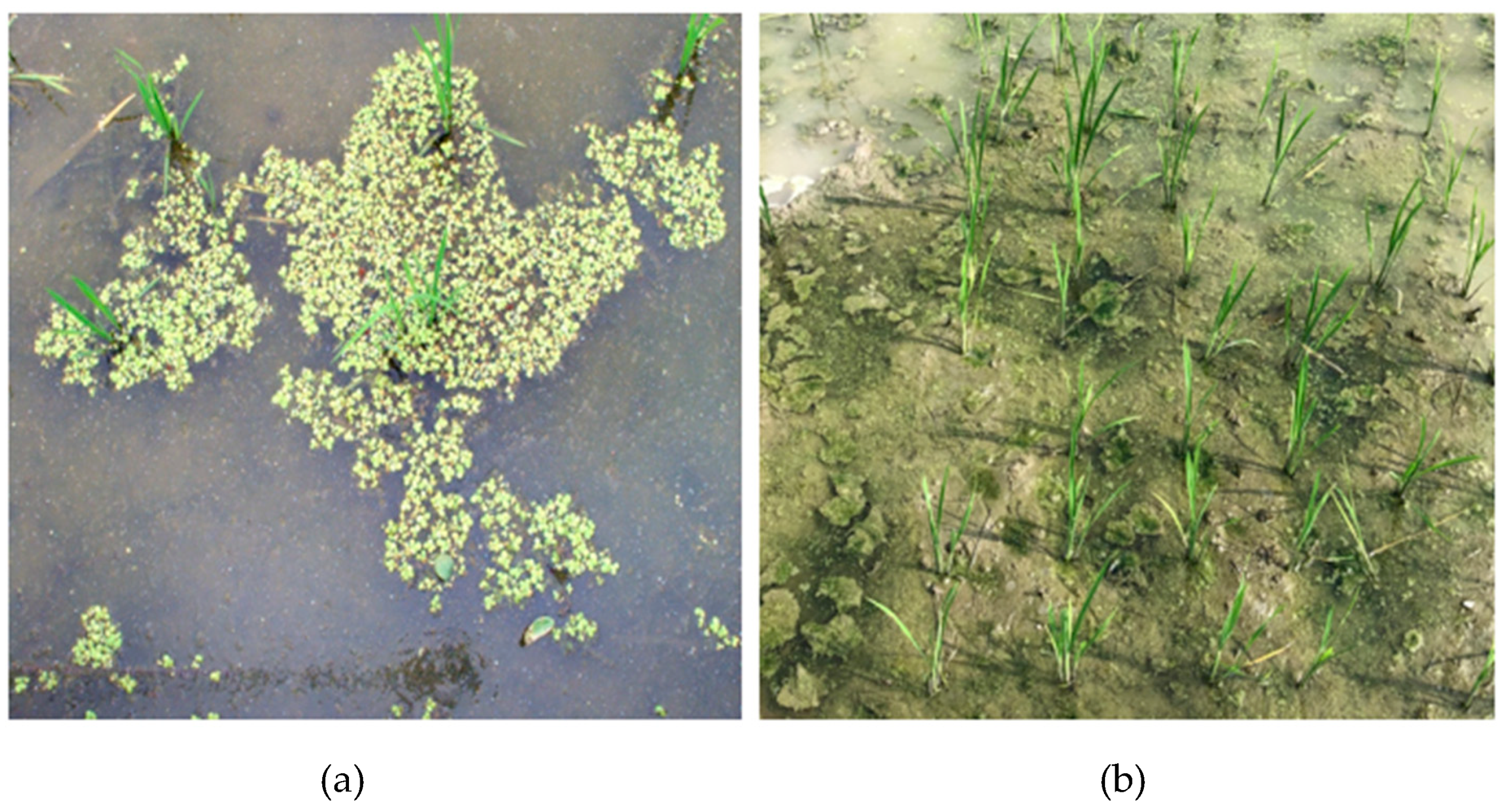
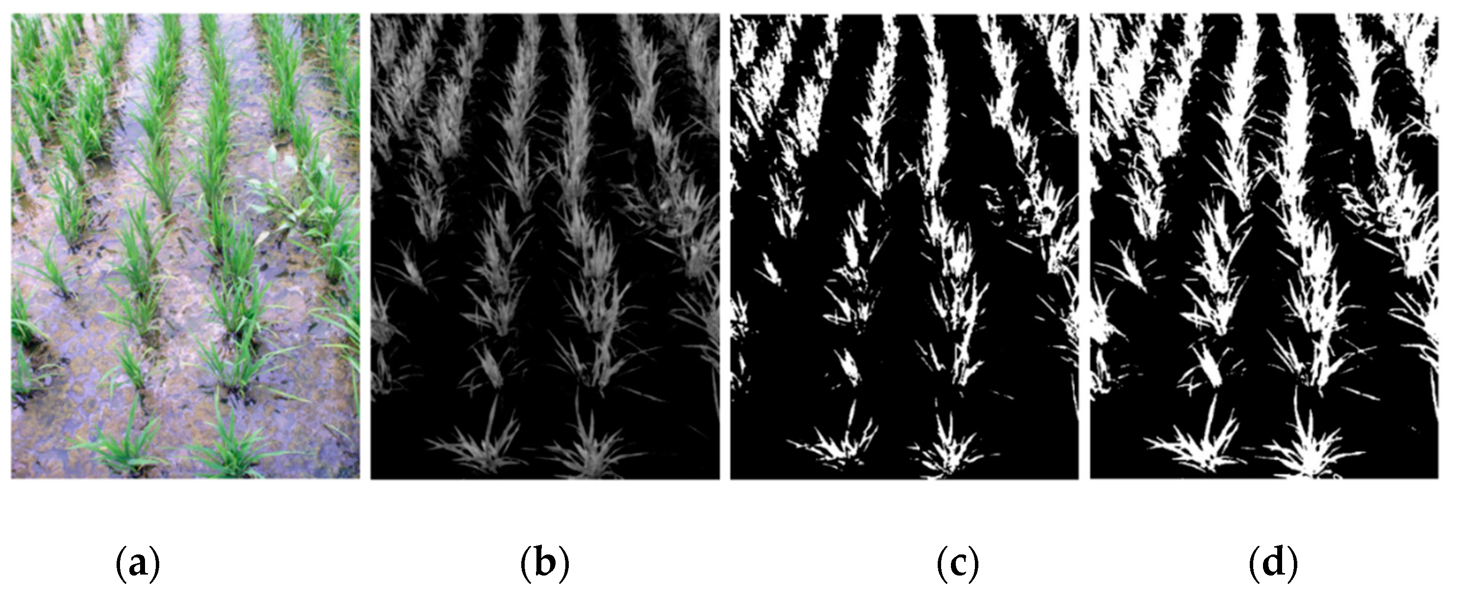
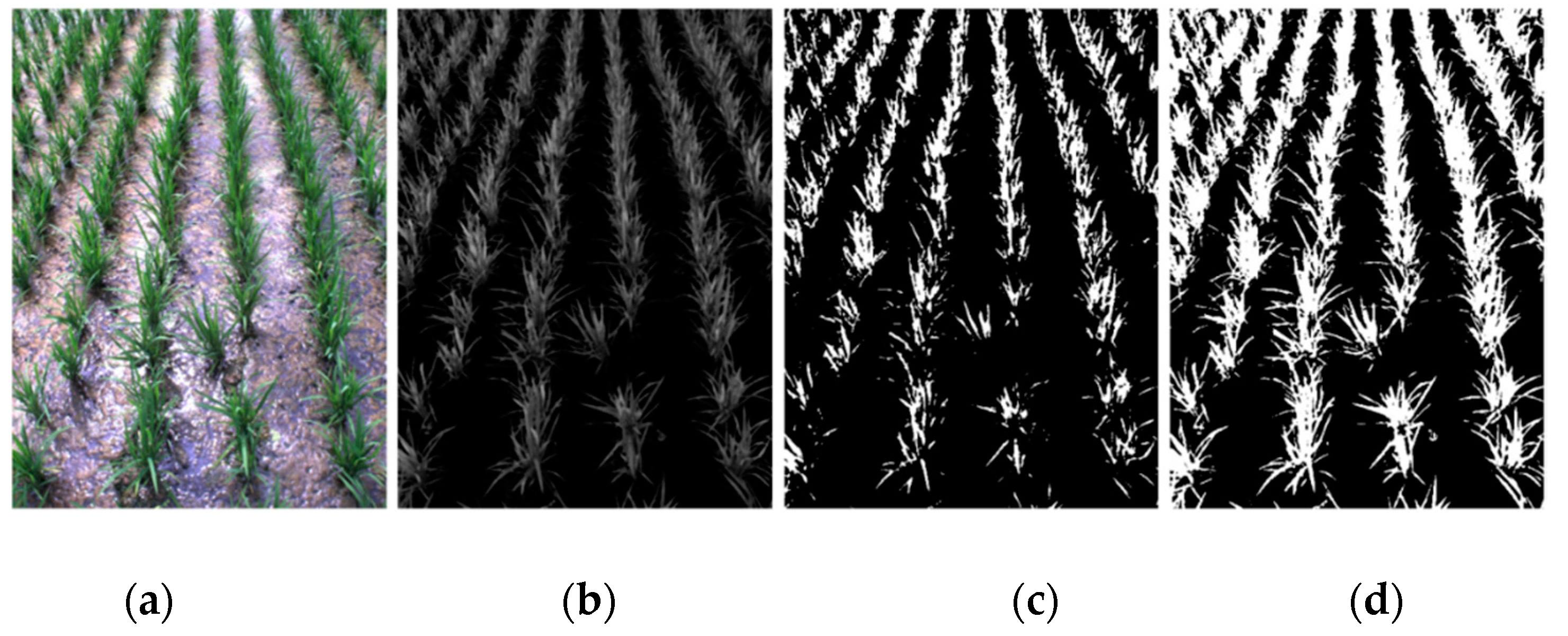
Figure 2a displays a typical image of a paddy field with duckweed.
Figure 2b displays the result of grayscale transformation by applying the
ExG index in
Figure 1a. After image binarization through a treble-classification Otsu method, green crops are identified as white pixels and green distractors are significantly removed, as shown in
Figure 2c. Lastly, the filtering operation is performed, and the result is as shown in
Figure 2e. In contrast, the result of image binarization through the typical Otsu method is shown in
Figure 2d, and the result of the filtering operation after the typical Otsu method is shown in
Figure 2f.
2.2. Feature Point Extraction
In the process of image processing, every step is applied to refine the information attached to the image. The essence of refinement is to ensure that the remaining information is effective and the useless information is eliminated. Until now, the binary image obtained after morphological operation, in which the white connected domain represents green crops, has already roughly displayed the position of the crop rows. To further determine the location of the crop rows through quantitative assessment, the white connected domain should be identified as a serial of feature points with exact coordinates, which is called feature point extraction.
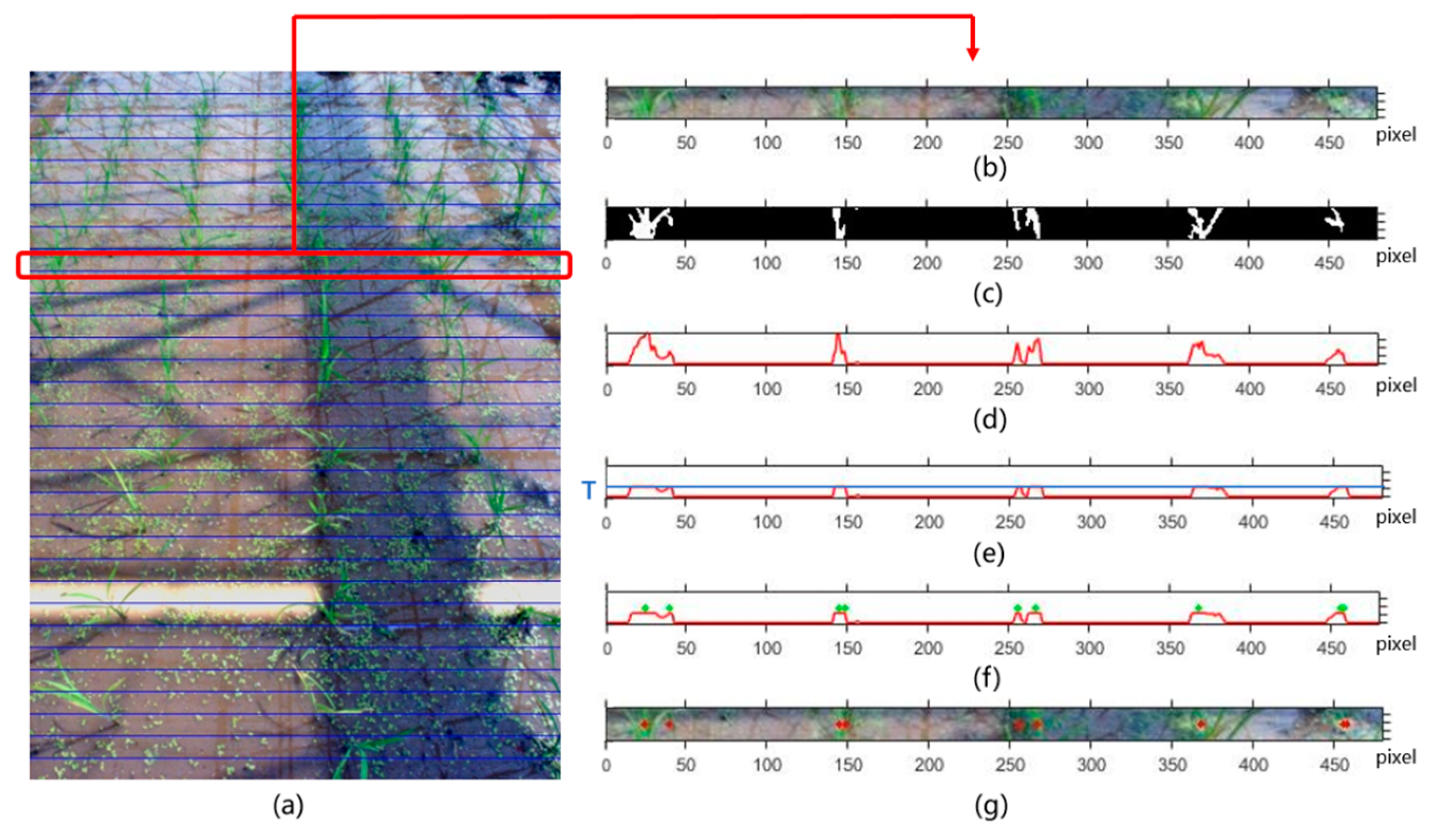
Considering that the noise attached to the obtained binary image is not significant, the horizontal strip method [
6], which determines the feature points by investigating the number of white pixels on each horizontal strip, is applied. The size of the binary image is assumed as
, where
denotes the height of the image while
denotes the width of the image, and the binary image is divided into
N strips. In order to appropriately reduce subsequent calculations, the size of each horizontal strip can be expressed as
, where
denotes the height of the strip and
. According to Zhang et al. [
34], 30 horizontal strips can provide a good result for a wide variety of conditions. In this paper, to match 30 horizontal strips,
h was adopted as 20. For each point of the binary image,
) denotes the gray value of point
For the points on the medial horizontal line in each horizontal strip, the number of white pixels at each column
is denoted as
[
34], as shown in Equation (21).
where
k denotes the index of horizontal strips.
Theoretically, if
, it means that the set of pixels in the
-th column on the
-th horizontal strip shows implicit crop information, but the feature point cannot be determined accordingly. The small patches of white pixels actually representing noise may be mistaken for feature points, since the area of the horizontal strip where only noise exists would also provide a positive
. Thus, some restrictions should be imposed on the judgement of feature points. To prove that it is reliable to recognize a certain area as a feature point, the information of green crops attached to the area should be relatively bigger; thus, the
of the area should be higher than a given threshold
, as shown in Equation (22).
where
is the thresholding coefficient with value
, and
is the natural logarithm.
Due to the clairvoyant principle of three-dimensional space, the densities of crop rows above and below the image are slightly different. To make the threshold
adaptive to every horizontal strip,
is constructed as a monotone increasing function, for the crop row in the upper part of the image is narrower while the lower part is wider. Through the threshold
, each column of pixels in the
-th horizontal strip is traversed, but the result is a series of intervals, not points. The next step is to find the starting and ending points of these intervals, and the midpoints between the starting and ending points are the feature points. A judge function
is defined to search the boundary points of these intervals, as shown in Equation (23).
If
, the abscissa of the starting point of a certain interval in the
-th horizontal strip is
. If
, the abscissa of the ending point of a certain interval in the
-th horizontal strip is
. Each start point and the next adjacent end point form an interval, and the midpoint of them can be identified as a feature point. In
Figure 3, all steps mentioned to extract feature points are illustrated.
2.3. Crop Row Detection
The feature points extracted from the binary image are scattered; hence, the next step is their classification based on coordinate information. In order to sort out these scattered feature points and dig out information of crop row position as accurately as possible, the proposed double-dimensional adaptive clustering algorithm is applied.
According to the principle and results of feature point extraction, it can be found that, in each horizontal strip, a single crop row may be identified with more than one feature point. That is, the feature points belonging to the same crop row have both horizontal and vertical extensions. Therefore, it is difficult to take the information of all these feature points into account at the same time if only the horizontal or vertical traversal is applied for clustering analysis. Additionally, there may be gaps in the distribution of feature points from the same crop row or pseudo feature points caused by green information distractors between two adjacent crop rows. In this case, the adoption of traditional clustering analysis will easily lead to over-clustering which means the feature points on the same crop row are divided into multiple clusters, or under-clustering which means the feature points that do not belong to any crop row are classified into a cluster of crop row. In the proposed double-dimensional adaptive clustering algorithm, firstly, a horizontal clustering analysis is performed, through which feature points in each horizontal strip are clustered according to their abscissa, and then a vertical clustering is performed to assign the horizontal clustering results to each corresponding crop row. This clustering method is proposed according to the relative positions between the feature points and the approximate direction of the crop rows in the image; therefore, prior knowledge about the number of crop rows is not required.
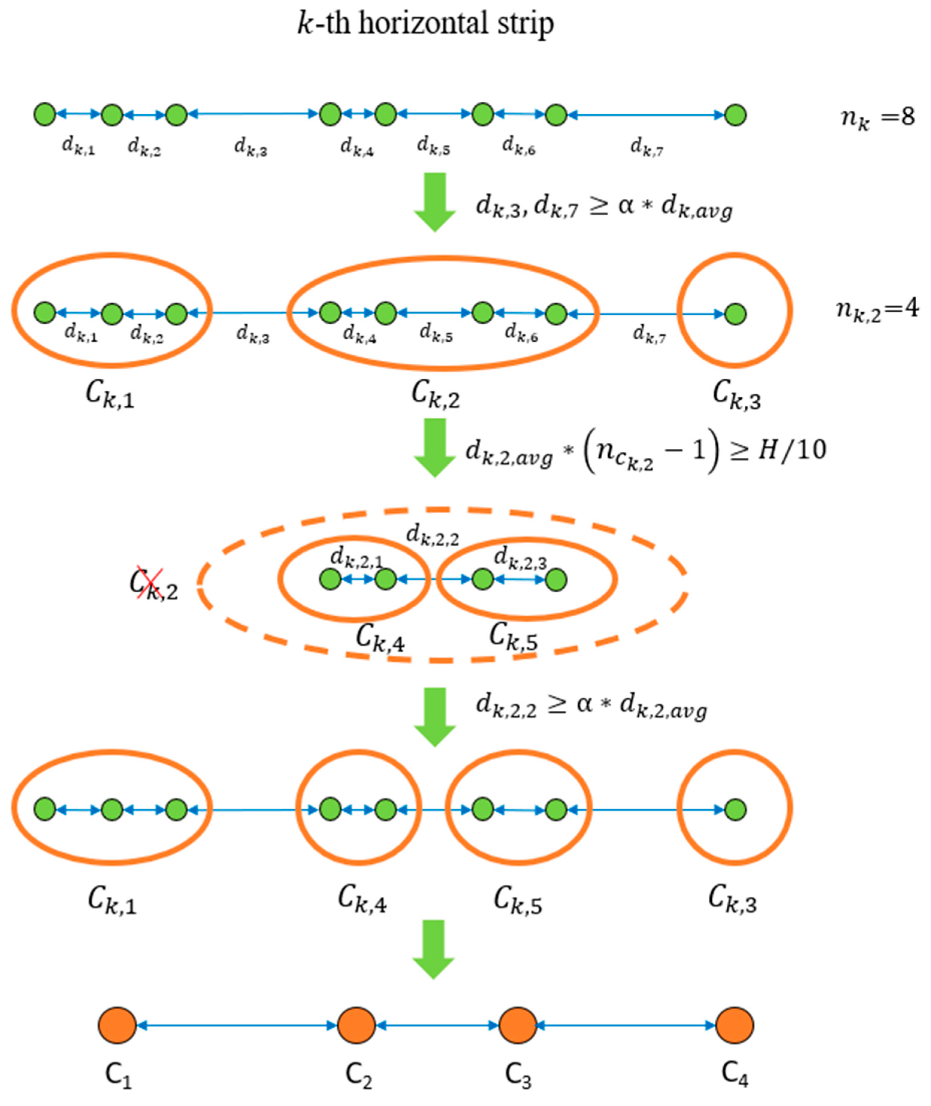
In horizontal clustering, a horizontal strip formed in the feature point extraction step is used as a unit to traverse. Initially, each feature point in a horizontal strip represents a single cluster. Now that the number of feature points in the
-th horizontal strip is assumed to be
(
), and
(
) denotes the
-th feature point of the
-th horizontal strip, then the distance between adjacent feature points in the same horizontal strip can be expressed as
(
), and the average distance between all these adjacent feature points is expressed as
, as shown in Equation (24).
The number of clusters in the
-th horizontal strip is assumed as
(
).
(
,
) denotes the
-th cluster of the
-th horizontal strip.
denotes the number of feature points in
, and
(
) denotes the
-th feature point in
. The distance between adjacent feature points in
can be expressed as
(
) and the average distance between all these adjacent feature points is expressed as
, as shown in Equation (25).
All the feature points are scanned from left to right in each horizontal strip, and the horizontal strips are scanned from top to bottom. In each horizontal strip, all feature points are traversed and, according to the relative position, feature points that meet the clustering conditions are merged. The above process is repeated until there is no incomplete clustering. The procedures of the horizontal clustering method are shown in
Figure 4. The specific steps of the horizontal clustering method are as follows:
Initialize .
For the -th horizontal strip, determine the value of . If , skip to step 9. If , calculate .
For the first feature point in each horizontal strip, initialize , make , and push into it. Make . Make , .
Define as the current feature point. Define as the current cluster. Calculate the distance between and the next adjacent feature point If , push into and make . If , make , initialize , push into and make . Practical experience has shown that 0.8 is suitable for .
Make . If , return to step 4. If , the first round of the -th horizontal clustering is completed. Record at this time as . Make .
If , skip to step 9. Define as the current cluster, and then calculate . If , make and repeat step 6. If , make and define as the current feature point. Initialize .
Calculate the distance between and the next adjacent feature point If , push into and make . If , make , initialize , make , push into , and make . Practical experience has shown that 0.8 is suitable for .
Make . If , return to step 7. If , make . Return to step 6.
Make . If , return to step 2. If , the horizontal clustering method ends.
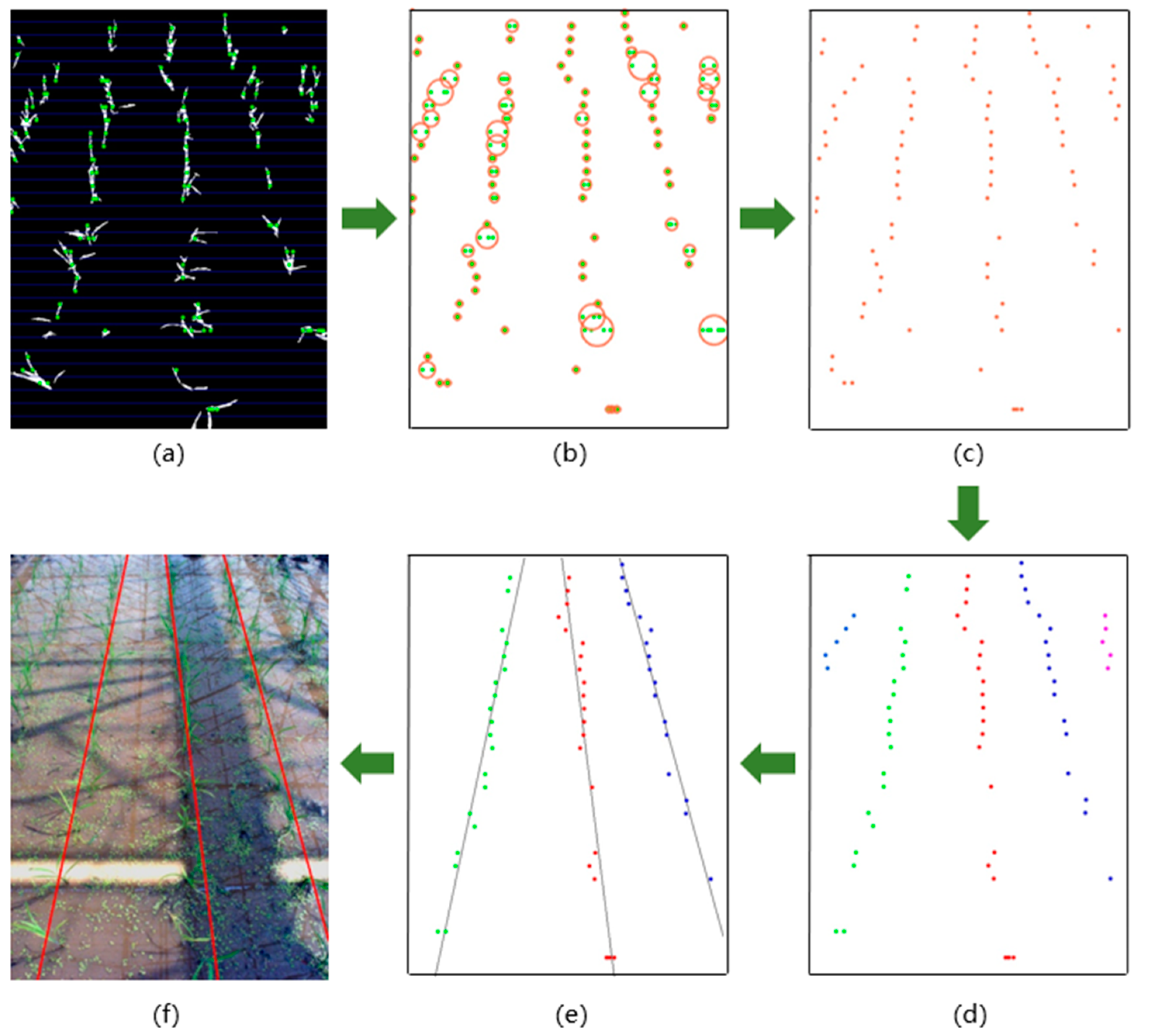
In this manner, the feature points on each horizontal strip are clustered on the basis of their relative position of the abscissa, and the mean value
of the abscissa of feature points in
is regarded as the abscissa of a new feature point, as shown in
Figure 5. After the horizontal clustering, feature points belonging to the same crop row are merged into new feature points horizontally. For each crop row, there is nearly only one new feature point remaining in each horizontal strip, and the current distribution of new feature points makes the crop rows appear clearer.
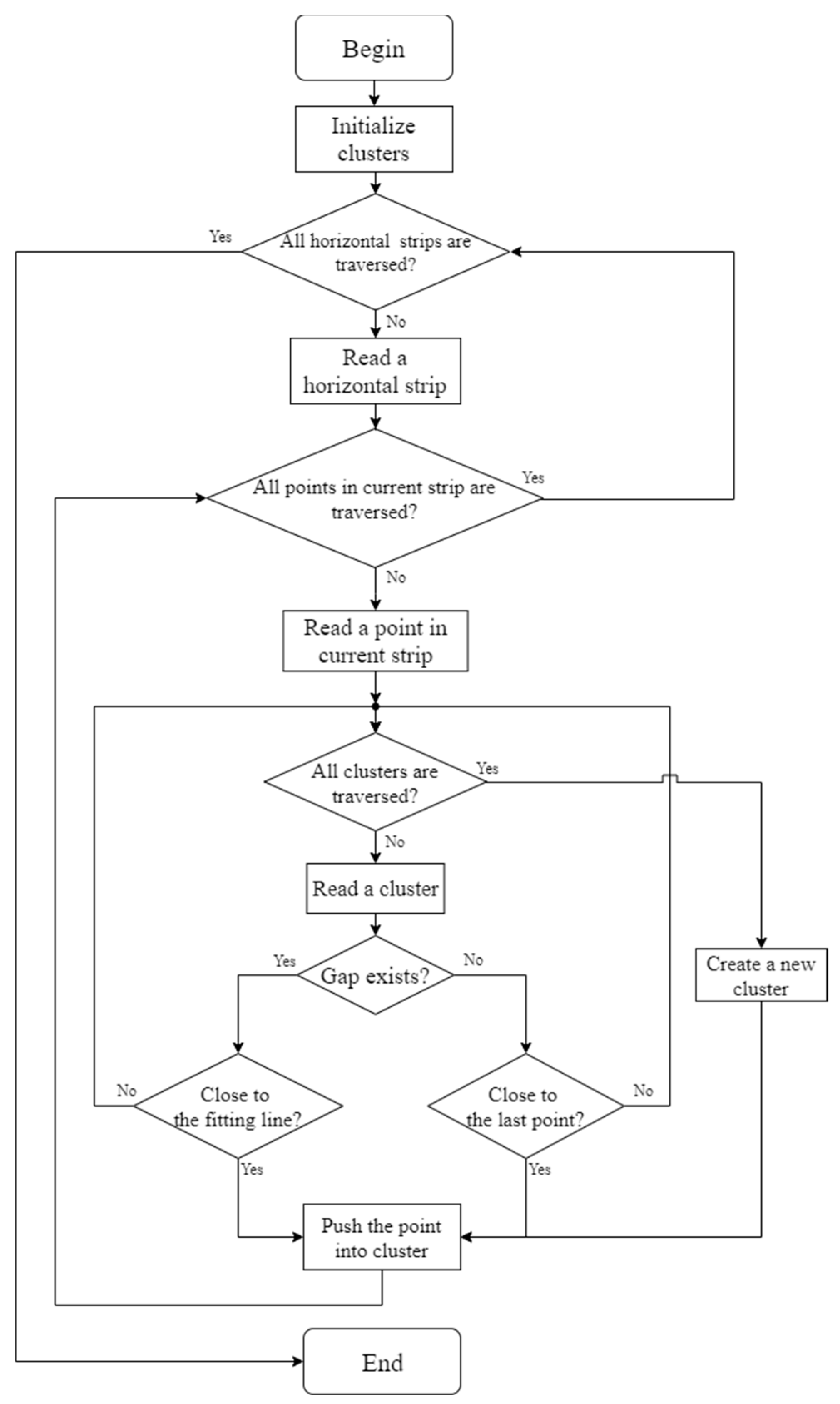
Vertical clustering is applied to new feature points, i.e., the results of horizontal clustering. Since the pitch angle of the camera is 60°, the closer to the top of the image, the closer the distance between crop rows, and the closer to the bottom of the image, the farther the distance between crop rows. For each cluster, the selection of an initial feature point is pivotal. To achieve better results at the initial stage, the vertical clustering is performed from bottom to top.
Make
denote the number of clusters, and make
(
) denote the
-th cluster of crop row. In vertical clustering, once a new feature point is pushed into
, the fitting line parameters of the feature points in
need to be calculated using the least square method. Make
denote the number of feature points of the
-th horizontal strip, and make
(
) denote the
-th feature point of the
-th horizontal strip. Make
denote distance between
and the last point in
, and make
denote distance between
and the fitting line of
. The thresholds of
and
are represented as
and
. If the ordinate distance between the current feature point and the last point in
is greater than
, this situation is defined as a gap. The basic judgment of vertical clustering is divided into two cases according to whether or not a gap is encountered. If a gap is encountered,
is the judging criterion. If there is no gap,
is the judging criterion. If
or
, the current feature point is pushed into the current cluster
. For a feature point, after traversing all the existing clusters and finding that none meets the judgment criterion, initialize a new cluster and push this feature point into it. Lastly, filter out those clusters with fewer than six feature points. The process of the vertical clustering method is shown in Algorithm 1, and the flow chart is shown in
Figure 6.
| Algorithm 1. The process of the vertical clustering method. |
Input: which denotes the number of horizontal strips.
which denotes the number of feature points of the k-th horizontal strip.
) which denotes the collection of feature points.
Outputs: Horizontal clusters ). |
1: initialize l = 1, =
2: for k = n: 1 |
| 3: for m = 1: |
| 4: for l = 1: |
| 5: if gap |
| 6: |
| 7:
|
| 8: continue |
| 9: else |
| 10: |
| 11: |
| 12: continue |
| 13: , |
| 14: |
4. Discussion
From the results of accuracy validation tests of the treble-classification Otsu method, it is clear that crop information is better distinguished and preserved in the binary image using treble-classification Otsu method. Under paddy field environments with strong interference, the grayscale image actually comprises three kinds of objects: background (non-green parts such as clear water), green distractors (duckweed, light-green weeds, and the water surface during eutrophication), and real rice seedings. Due to their different degrees of green color, these three kinds of objects obtain different degrees of gray values. Thus, the treble-classification Otsu method divides the pixels in the greyscale image into three clusters according to their gray value, in order to distinguish the green distractors and real crops. The typical Otsu method only divides the pixels into two clusters: foreground and background; therefore, the green distractors will mix into the real crops, together in the foreground. The experimental results and analyses mentioned above verified that, under various interference environments, the treble-classification Otsu method has superior performance to the typical Otsu method.
During the efficiency validation tests of the treble-classification Otsu method, the average value of time consumed in calculating the threshold through the treble-classification Otsu method was slightly larger. By analyzing the theories of the two methods, it can be found that treble-classification Otsu requires more nested loops compared to typical Otsu; hence, the amount of calculation is larger, which will inevitably lead to lower efficiency. From the results in
Table 1, it can be concluded that, when the size of images matches the industrial requirements for visual navigation [
34], although the efficiency of the treble-classification Otsu method is inevitably lower, the deviation of time consumed through the two methods is small enough and can definitely meet the efficiency requirement of visual navigation.
Under the perspective of qualitative analysis, the crop row detection method achieved good visual results, as shown in
Figure 10. However, the quantitative measurement of the detection accuracy is not quite straightforward because it is difficult to get true position and direction for the center lines of crop rows due to natural variations in the crop growth stage [
13]. To establish a quantitative evaluation standard, a simple evaluation method is proposed.
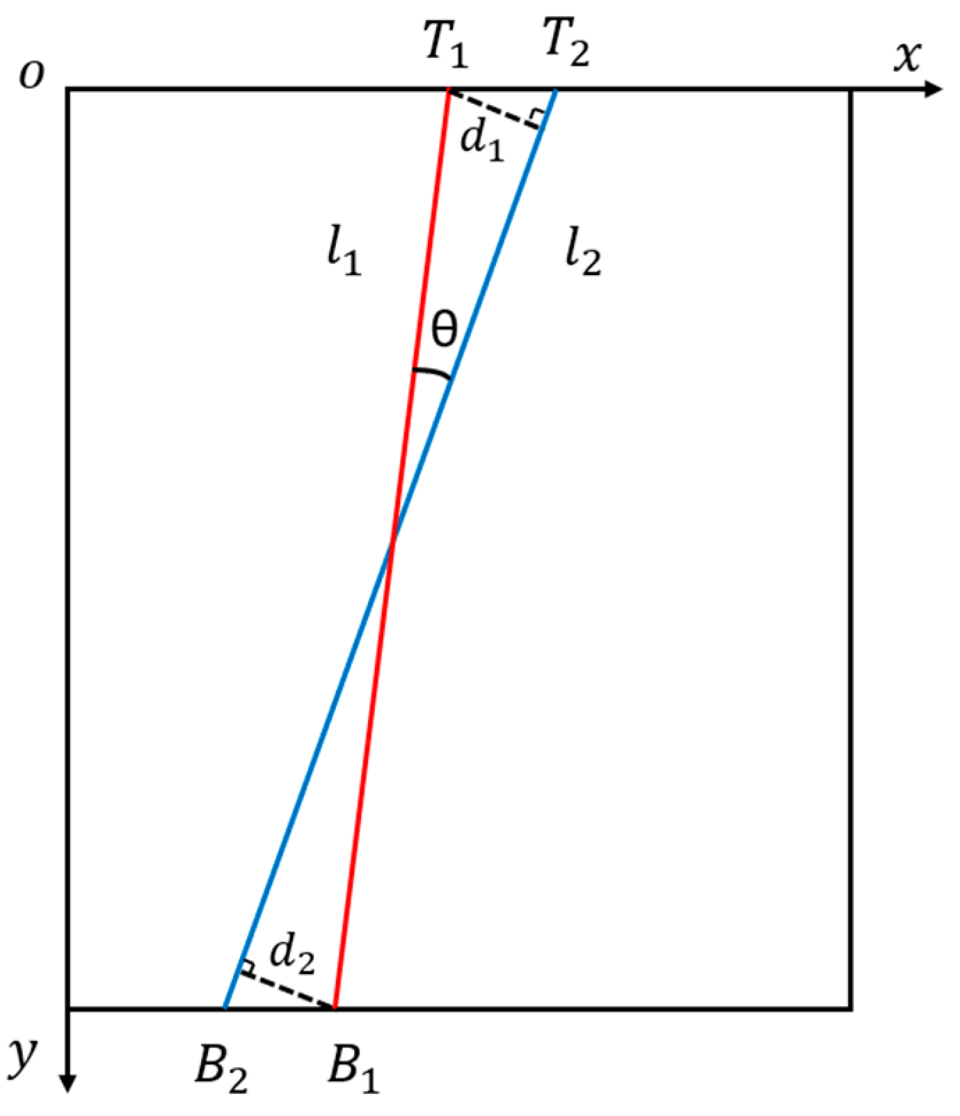
A schematic diagram of the mechanism is given in
Figure 11. In an image, assume that line
is a straight line which has been detected and line
is a known correct line of the same crop row. The straight line
intersects the upper and lower boundaries of the image at two points
and
, while
intersects the upper and lower boundaries of the image at
and
. In order to rigorously evaluate the similarity between these two line segments, the evaluation of both angle and distance should be considered. Make
denote the angle between
and
. Make
denote the distance between
and
. Make
denote the distance between
and
. The linear equations of
and
are assumed as follows:
where
and
are the slopes of
and
respectively, and
and
are the
y-intercepts of
and
, respectively. Then, the calculation formula of
can be expressed as
is used to evaluate the similarity of postures of
and
. A smaller value of
denotes more similar postures of
and
. The calculation formulas of
and
can be expressed as
where
and
are the horizontal and vertical coordinates of respectively, and
and
are the horizontal and vertical coordinates of
, respectively. In order to combine the results of
and
, make
denote the average of
and
. A smaller
denotes that
and
are closer in the distance scale. The calculation formula of
can be expressed as
Due to the complexity of a paddy field, traditional methods do not work well for crop row detection. Thus, the known correct crop lines can be drawn by experts to establish accuracy criterion. The quantitative evaluation method can be used to compare the results of the proposed crop row detection method and the results of an expert. As a comparison, experiments of crop row detection using the method based on typical Otsu were also conducted. The method based on typical Otsu used an image processing flow similar to the proposed method. The only difference between the two methods was the binarization process, whereby the proposed method used treble-classification Otsu and the traditional method used typical Otsu.
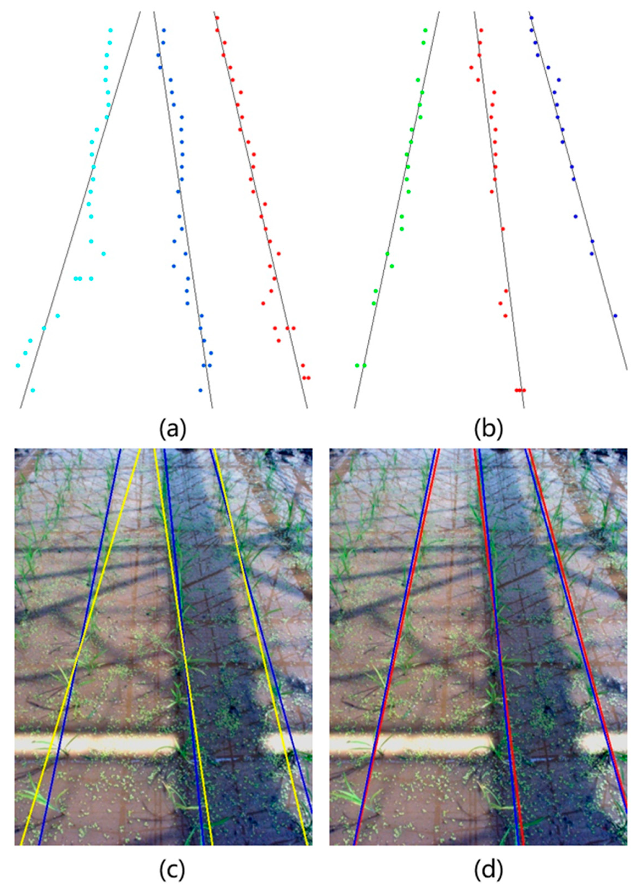
The comparison results and accuracy of the proposed method and detection method based on typical Otsu in eutrophication condition are presented in
Figure 12 and
Table 2. The average value of
and the average value of
of each crop row detected under eutrophication conditions are presented. Obviously, the proposed method was better than the traditional method in terms of the quantitative accuracy index. From the images of crop row detection based on valid clusters, it can be found that the proposed method finished the clustering process by fewer valid points than the method based on typical Otsu. The method based on typical Otsu retained more valid feature points, but these valid points were not enough to represent the position information of the crop rows. Thus, the final results of traditional method were relatively poor. However, since the proposed method has higher screening requirements, when the image quality is not high enough and the number of feature points that can be screened out is small, the detection accuracy is likely to be greatly reduced. In contrast, the method based on typical Otsu can retain more feature points; therefore, the detection accuracy is relatively stable.
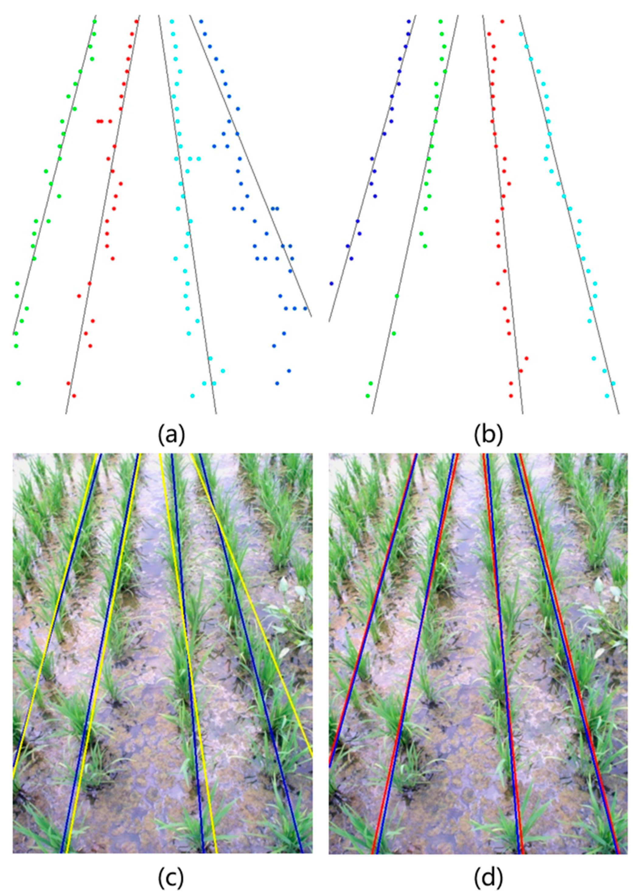
The comparison results and accuracy of the proposed method and detection method based on typical Otsu with disturbed weed are presented in
Figure 13 and
Table 3. The average value of
and the average value of
of each crop row detected with disturbed weed are presented, and the proposed method is shown to be better than traditional method in terms of the quantitative accuracy index. From the images of crop row detection based on valid clusters, it can be found that feature points of the traditional method were more susceptible to interference by disturbed weed. The area where the disturbed weed was located was mixed with the crop row area, which affected the accuracy of crop row detection.
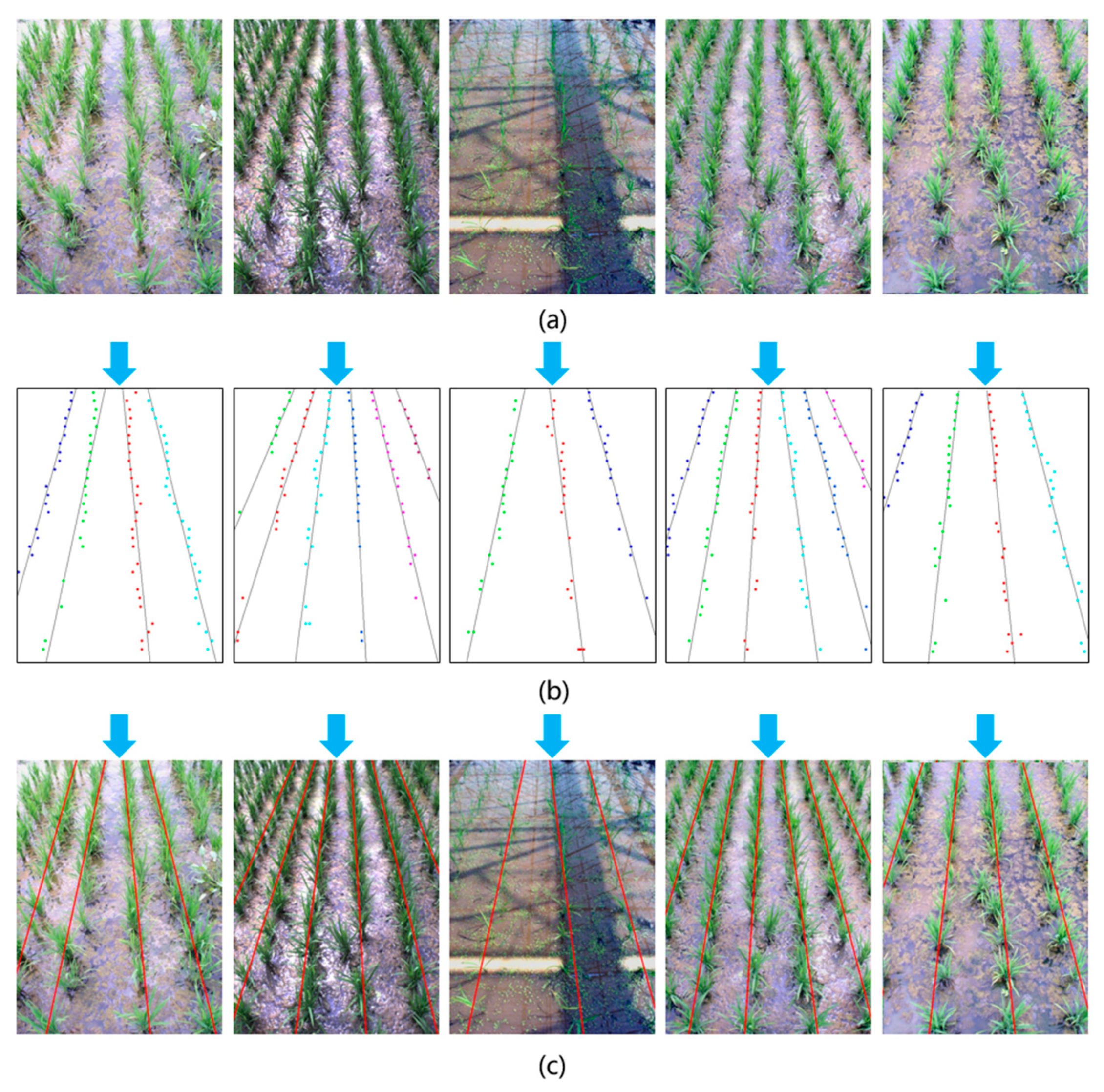
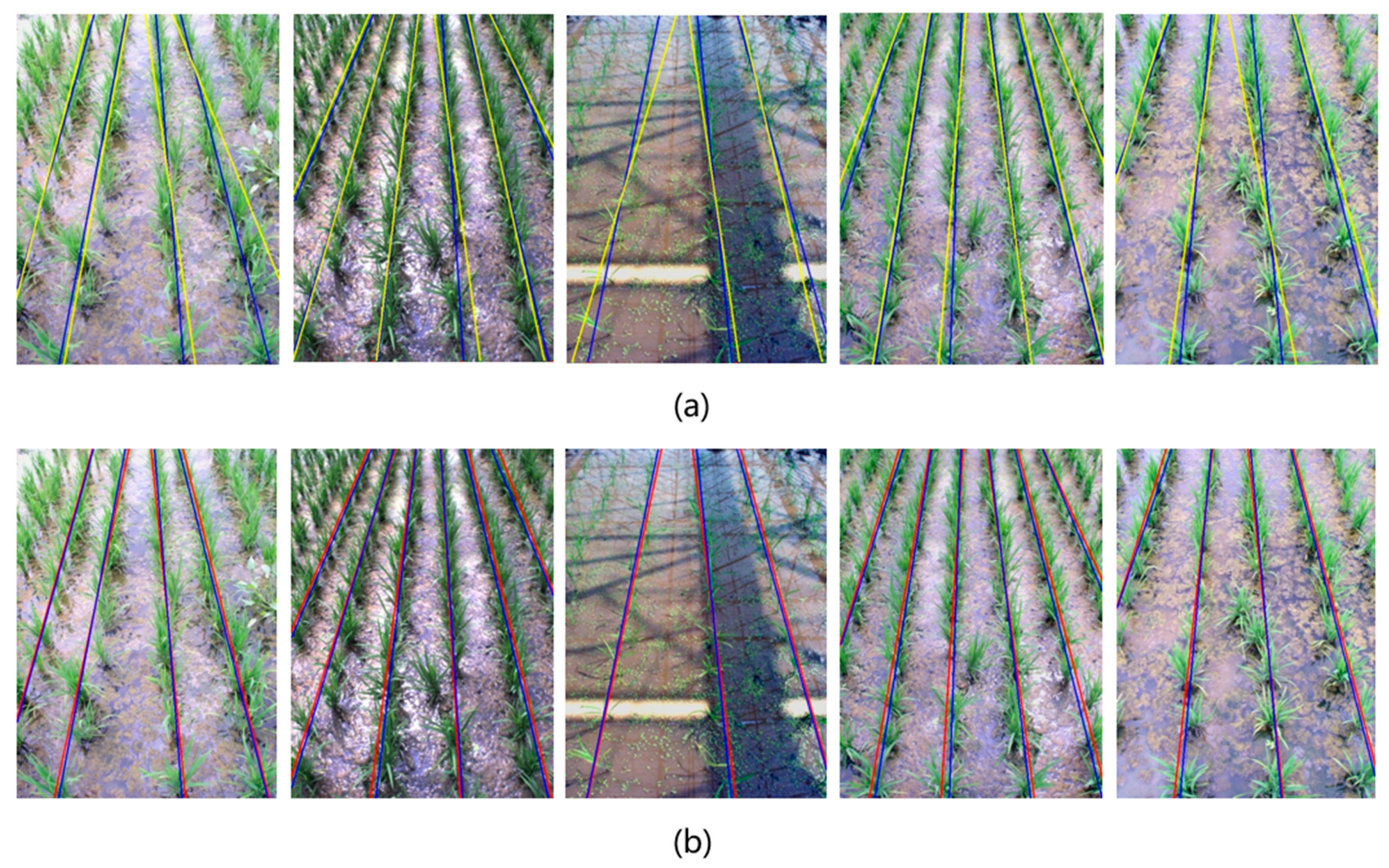
The comparison results of five illustrative images under various conditions are shown in
Figure 14. In this research, to get more convincing results, 60 images of three different conditions were tested, and the results are shown in
Table 4.
In
Table 4, the average value of
and the average value of
of each crop row detected under three different conditions are presented. Through quantitative analysis, it can be seen that the detection accuracy under weak interference was the highest among all three conditions, and this is consistent with our expectation. For a total of 60 images, the average values of
and
were within 0.02° and 10 pixels, respectively. The results of the detection method based on the typical Otsu method are also shown in
Table 4. For the traditional method, although good results could be achieved under weak interference, the accuracy increasingly declined when interference increased. The proposed method performed better than traditional method especially under strong interference.
Compared with previous studies [
3,
34], the proposed method does not require prior knowledge about the number of crop rows and does not occupy a lot of computing resources. As a result of the proposed method, the screening criteria for feature points are indirectly improved. Therefore, the field of view of the image to which this method is applicable should not be too narrow; otherwise, it would be more susceptible to interference from local extreme values than traditional methods. In short, it can be inferred from the quantitative results that, after applying the treble-classification Otsu method, the proposed feature point extraction method and the clustering algorithm could achieve better performance than the method based on typical Otsu under various interferences.


 and
and 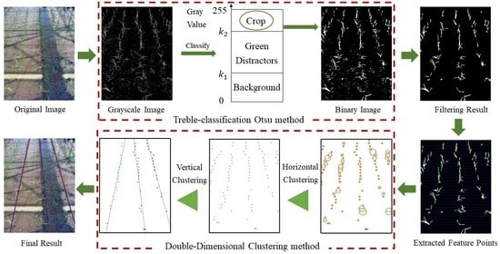


