Article

Simplified Priestley–Taylor Model to Estimate Land-Surface Latent Heat of Evapotranspiration from Incident Shortwave Radiation, Satellite Vegetation Index, and Air Relative Humidity

1
Faculty of Geographical Science, Beijing Normal University, Beijing 100875, China
2
State Key Laboratory of Remote Sensing Science, Jointly Sponsored by Beijing Normal University and Institute of Remote Sensing and Digital Earth of Chinese Academy of Sciences, Beijing 100875, China
*
Author to whom correspondence should be addressed.
Submission received: 11 January 2021 / Revised: 13 February 2021 / Accepted: 24 February 2021 / Published: 27 February 2021
(This article belongs to the Special Issue Disruptive Trends of Earth Observation in Precision Farming)

Abstract

:
An operational and accurate model for estimating global or regional terrestrial latent heat of evapotranspiration (ET) across different land-cover types from satellite data is crucial. Here, a simplified Priestley–Taylor (SPT) model was developed without surface net radiation (Rn) by combining incident shortwave radiation (Rs), satellite vegetation index, and air relative humidity (RH). Ground-measured ET for 2000–2009 collected by 100 global FLUXNET eddy covariance (EC) sites was used to calibrate and evaluate the SPT model. A series of cross-validations demonstrated the reasonable performance of the SPT model to estimate seasonal and spatial ET variability. The coefficients of determination (R2) of the estimated versus observed daily (monthly) ET ranged from 0.42 (0.58) (p < 0.01) at shrubland (SHR) flux sites to 0.81 (0.86) (p < 0.01) at evergreen broadleaf forest (EBF) flux sites. The SPT model was applied to estimate agricultural ET at high spatial resolution (16 m) from Chinese Gaofen (GF)-1 data and monitor long-term (1982–2018) ET variations in the Three-River Headwaters Region (TRHR) of mainland China using the Global LAnd-Surface Satellite (GLASS) normalized difference vegetation index (NDVI) product. The proposed SPT model without Rn provides an alternative model for estimating regional terrestrial ET across different land-cover types.

Graphical Abstract

1. Introduction

Latent heat of evapotranspiration (ET) observations and simulations are crucial in monitoring the energy and water cycle among different land-surface ecosystems [1,2,3,4]. Especially in typical eco-environmentally vulnerable areas, ET is affected by serious surface dry status resulting in a food and water resources crisis as well as eco-environment deterioration [5,6,7,8]. It is tough to accurately simulate regional ET because of the heterogeneous surface and complicated biophysical properties [9]. Moreover, at large scale, sparse ground observations (e.g., eddy covariance flux towers) limit accurate estimation of spatiotemporal ET distribution.
Satellite remote sensing is the most important approach for acquiring regional water fluxes because it has improved regional-scale estimates of land-surface parameters linked to ET (e.g., surface net radiation, Rn; leaf area index, LAI; normalized difference vegetation index, NDVI; soil moisture, SM; land-cover types and albedo) [10,11,12]. Over the past 40 years, many satellite-derived ET approaches have been developed to simulate regional water fluxes [13,14,15,16,17,18,19]. Generally, these ET approaches include: (1) statistical models developed by building the relationship between ground-measured ET and satellite-derived biophysical variables using calibration datasets that are considered to be the behaviors of ET process [2,20,21,22]; (2) physical models that involve the energy balance models using thermal land-surface temperature (LST) data [19,23,24,25], Penman–Monteith (PM) as well as its simplified version—Priestley–Taylor (PT) models—using optical satellite vegetation parameters [10,16,17,26,27]; and (3) data assimilation models that assimilate satellite-derived biophysical variables into distributed hydrologic models for improving ET estimation [28,29]. Although these models have been successfully applied to monitor regional terrestrial ET, their estimation results might differ greatly because of differences in model structures and input parameters [30,31,32].
As an appealing model, the hybrid PT model (a joint physical and empirical model) with ideal coefficients calibrated using satellite and ground-measured variables yields reliable water flux estimates over different large-scale regions. [1,27,30,33,34]. In general, hybrid PT models use the potential ET (PET) to multiply the combination of ecophysiological constraints (e.g., LAI and NDVI) and meteorological variables for estimating ET. For instance, Wang et al. [21] incorporated vegetation influence on ET and developed a simple ET model using ground-observed Rn, air temperature and satellite-derived NDVI data over Southern Great Plains (SGP) of the US. However, this model cannot include the effects of SM on ET during drought conditions. Wang and Liang [12] introduced the diurnal air temperature range (DaTR) for characterizing the impacts of SM on ET to estimate ET. Recently, Yao et al. [22] proposed a hybrid ET model by replacing SM with air relative humidity (RH) in the Heihe River (HR) basin over Northwest China.
Although the above hybrid PT models from different parameterization schemes have higher performance than PM models because of their good universal physical theory, the fixed parameters of these ET models could lead to large errors when they are applied uniformly to globally different biomes. In addition, the accuracy of all these models is highly relied on the results of the estimated Rn. Previous studies highlighted that Rn could be reliably estimated from incident shortwave radiation (Rs), minimum air temperature (Tmin), RH and NDVI [35,36]. Therefore, ET may be directly derived from Rs, Ta, Tmin, RH and NDVI by avoiding Rn estimation while hybrid PT models require further parameter calibration in different ecosystem types. Yet, there is no similar studies to develop a simplified PT model with ecophysiological constraints calibrated to measurements from global EC, satellite-derived NDVI, Rs, and other meteorological observations across different land-cover types.
In this study, a simplified Priestley–Taylor (SPT) model was developed to estimate global terrestrial evapotranspiration across different land-cover types by combining Rs, satellite vegetation index, and air RH. The objectives here were to (1) design the SPT model to optimize the coefficient using ground-measured ET, satellite-derived NDVI, Rs and other meteorological observations; (2) validate the SPT model based on a ten-fold cross-validation method across different land-cover types from global FLUXNET measurements at 100 flux tower EC sites; and (3) apply the SPT model for estimating agricultural ET at high spatial resolution from Chinese Gaofen (GF) -1 data and for monitoring long-term (1982–2018) ET variations in the Three-River Headwaters Region (TRHR) of China.

2. Data and Case Study

2.1. Data for Model Development

EC measurements and corresponding meteorological observations were used to develop and evaluate the ET model. The data were obtained from LathuileFlux, AsiaFlux, AmeriFlux, ChinaFlux, and Chinese Ecosystem Research Network (CERN) from FLUXNET network at 100 sites situated in Europe, Asia, and North America, two sites located in Africa, three sites located in South America and three sites located in Australia (Figure 1). The climate types of the sites range from arctic to tropical and from dry to humid. The plant function types for the sites included cropland (CRO, 11 sites), grassland (GRA, 11 sites), deciduous broadleaf forest (DBF, 11 sites), evergreen broadleaf forest (EBF, 11 sites), deciduous needleleaf forest (DNF, 4 sites), evergreen needleleaf forest (ENF, 11 sites), mixed forest (MIF, 11 sites), shrubland (SHR, 11 sites), savanna (SAW, 9 sites), and wetland (WET, 10 sites).
The observed data contain half-hourly ET, sensible heat flux (H), Rs, Rn, air temperature (Ta), Tmin, RH and wind speed (WS). The daily and monthly variables were also linearly aggregated from the half-hour means. When the amount of missing daily data was more than 25% of the observations, the daily values were set as missing. The fixed Bowen ratio (BR) method designed by Twine et al. [37] was used to revise ET due to the unclosed energy budget.
ET = ET ori R BR
R BR = E T ori + H ori R n G
where ET is the revised evapotranspiration; ETori and Hori are the original ET and the H derived from EC observations, respectively; and RBR refers to the energy closure ratio.
To develop the ET model, the MODerate resolution Imaging Spectroradiometer (MODIS) NDVI products were used and they have a spatial resolution of 1-km and temporal resolution of 8-day. The eight-day NDVI averages were interpolated to daily values based on the linear interpolation method.

2.2. Case Study for Model Application

2.2.1. Case Study I

To illustrate the performance of the SPT model for estimating agricultural ET at a high spatial resolution from Chinese GF-1 data, the Huailai agricultural region of China was selected as a study area (Figure 2). The Huailai agricultural region (~7.8 km2) is situated between 40.3425°N–40.3621°N and 115.7774°E–115.8188°E and located in the HR Basin in northern China. The land cover is dominated by agriculture and presents small portions of other land-cover types (e.g., forest, grass, water, and barren land). Among the crops grown, the summer crop is mainly dominated by maize. Two flux tower sites, namely EC1 site (40.3491°N, 115.7880°E) and EC2 site (40.3574°N, 115.7923°E), were in the northwestern parts of this study area. The main plant function type for the two sites is continuous maize land. EC data measured between 2013 and 2017 also include half-hourly ET, H, Rs, G, Rn, Ta, Tmin, RH, VPD (vapor pressure deficit) and WS. The same procedure as for the EC data for model development was used to process these data.
Fifty-five Chinese GF-1 wide field view (WFV) images for 2013 to 2017 were used to calculate NDVI for ET estimation. The Chinese GF-1 satellite, launched on 26th April 2013, has produced 16 m images per 4 days with a continuous swath of approximately 800 km [38]. The GF-1 data have four bands. Band 1 is a blue band with a spectral range of 0.45–0.52 µm. Band 2 is a green band with a spectral range of 0.52–0.59 µm. Band 3 is a red band with a spectral range of 0.63–0.69 µm. Band 4 is a near-infrared band with a spectral range of 0.77–0.89 µm. The raw DN (digital number) values were released by the Chinese GF-1 data and ENVI software was used to conduct radiance calibration, atmospheric correction, and geometric correction.

2.2.2. Case Study II

The TRHR of China was also selected as another study area to assess the performance of the SPT model for monitoring long-term (1982–2018) ET variations using the Global LAnd-Surface Satellite (GLASS) NDVI product from Advanced Very High-Resolution Radiometer (AVHRR) data [39]. The TRHR (31.63°N–36.33°N, 89.52°E–102.23°E) is situated in southern parts of Qinghai Province (QH) of China and belongs to the hinterland of the Tibetan Plateau (TP) (Figure 2). TRHR is a famous region of the Lantsang, Yellow, and Yangtze rivers. Grassland (mainly alpine meadow) is the dominant ecosystem type of the TRHR. One grass flux tower site (Three-River Headwaters, TRH) (34.35°N, 100.55°E) was situated in the eastern parts of this study area. EC data measured between 2016 and 2017 also included half-hourly ET, H, Rs, G, Rn, Ta, Tmin, RH, VPD, and WS. The same procedure as for the EC data for model development was also used to process these variables.
To simulate the long-term evapotranspiration, the 8-day GLASS NDVI product with a spatial resolution of 0.05 degrees from 1982–2018 were used [39]. The 8-day NDVI data were linearly interpolated into daily values. The China Meteorological Forcing Dataset (CMFD) for daily Ta, Tmin, Rs, and RH for the period 1982–2018 were also used [40,41,42]. These meteorological variables (Ta, Tmin, Rs, and RH) were resampled into 0.05° from a 0.1° spatial resolution using linear interpolation.

3. Methodology

3.1. Simplified Priestley–Taylor Model

The ET model was developed based on the simplified PT (SPT) model in which Rs was chosen to substitute available energy (Rn-G) since Rn can be reliably derived from Rs and other environmental variables [36] and G (soil heat flux) can be calculated using Rn [8,12,27]. In the SPT model, the ET is calculated as:
ET = f ( c ) Δ Δ + γ R s
where refers to PT parameter under wet surface conditions (1.26); ∆ refers to the slope for saturated vapor pressure (SVP) curve; γ stands for psychrometric constant. f(c) is the environmental constraint that is determined by meteorological and satellite variables [10,22]. It is tough to accurately calculate f(c) because of the large uncertainties in the characterization of the dynamics of the ET process using limited satellite and meteorological variables [4,43]. Because temperature and water are the key environmental constraints for controlling the evaporation fraction (EF), i.e., the ratio of ET to available energy, a linear combination of Tmin, NDVI, and RH was introduced to estimate f(c).
f ( c ) = α 0 + α 1 T m i n + α 2 NDVI + α 3 R H
where αi (i = 0, 1, 2, 3) refers to the calibrated empirical coefficient (dimensionless) and varies among different land-cover types. In this model, Tmin represents the effects of temperature on EF, NDVI characterizes the vegetation transpiration influenced by temperature and water, and RH takes into account the contribution of SM on EF for a short period.
The merits of the SPT model over many other physical evapotranspiration approaches are that it (1) improves operability for estimating long-term ET since it only depends on Rs, Tmin, NDVI and RH; (2) uses a linear combination of Tmin, NDVI and RH to avoid aerodynamic and surface resistance and to reduce biases of the required forcing datasets [1,27]; and (3) improves the accuracy of estimating ET by taking into account the differences in the calibrated coefficients of Equation (4) for a variety of land-cover types.

3.2. Cross-Validation

The empirical coefficients of Equation (4) were calibrated using a linear regression based on the measured data (EC observations and NDVI data) for 100 flux towers. To evaluate the estimated ET accuracy, the performance of the SPT model was assessed based on a ten-fold cross-validation approach that randomly divided the data into ten groups with about equal numbers for samples [44]. The simulated ET was independently evaluated for every of the ten groups using the calibrated empirical coefficients of Equation (4) based on the data of the remaining nine groups. The bias, root-mean-square error (RMSE), coefficients of determination (R2), and p values of the simulated and observed ET were also used to illustrate the performance of the SPT model [45].
B i a s = 1 N i = 1 N ( S i M i )
R M S E = 1 N i = 1 N ( S i M i ) 2
R 2 = [ 1 N i = 1 N ( S i S ¯ ) ( M i M ¯ ) ] 2 1 N i = 1 N ( S i S ¯ ) 2 1 N i = 1 N ( M i M ¯ ) 2
where N is the number of samples, Si is the simulated ET for sample i, Mi is the ground-observed ET for sample i, S ¯ is the averaged S and M ¯ is the averaged M.
To assess the performance of the SPT model to simulate the spatial and temporal variations in ET, the ET variability was validated, including (1) seasonal variation and, (2) spatial (among-site) variation, and (3) annual anomalies, using estimated and ground-measured data. The seasonal (daily and monthly) estimated and ground-measured ET was first validated. The spatial (among-site) variation was then validated by comparing the average ET of the estimated and ground-measured ET at every site for the whole period. Finally, the annual ET anomaly for each site was calculated by removing the multiyear average from the annual ET values.
To facilitate comparisons with other ET models, the dataset was randomly stratified into two different groups for about equal numbers for samples, and entire sites were assigned to each group [44]. Daily ET was validated using datasets from one group using the calibrated parameters of Equation (4) based on data from another group.

3.3. Comparison to the PT-JPL Model

The revised Priestley–Taylor (PT) model from the Jet Propulsion Laboratory (PT-JPL) was developed based on the original PT equation by introducing ecophysiological constraints (NDVI and LAI) and atmospheric constraints (RH and VPD) to estimate terrestrial ET [1,10]. The validation for 16 global EC sites illustrates that the PT-JPL model accounts for 90% of ET variations, and comparisons with multiple models indicate that this model is the most promising ET method model [30,46]. An obvious difference between the SPT model and PT-JPL is that the SPT model uses ground measurements to calibrate the coefficients of the ecophysiological constraints to develop f(c) for different land-cover types.

4. Results

4.1. Model Parameterization

Long-term (2000–2009) ground measurements and the corresponding NDVI datasets for different land-cover types were analyzed at 100 flux tower sites to detect the driving variables for determining terrestrial ET. Table 1 illustrates the correlation coefficients (r) between ET and Rs, Tmin, RH, and MODIS NDVI for different land-cover types. For all land-cover types, Rs presented the highest R2 with ET (0.20 ≤ R2 ≤ 0.56) and Tmin presented the second highest (0.17 ≤ R2 ≤ 0.53), demonstrating that both Rs and Tmin are the dominant variables driving terrestrial ET. The NDVI was also highly correlated with ET, with R2 varying from 0.16 to 0.50 for most land-cover types (except for WET), which illustrates that the NDVI is an important variable controlling the variation of terrestrial ET. The NDVI characterizes vegetation amounts and reflects vegetation transpiration by coupling CO2 assimilation with vegetation photosynthesis [47]. The R2 values between RH and ET were relatively low (less than 0.11) for all land-cover types due to the seasonal variability of RH.
To parameterize f(c) of the SPT model, correlation coefficients (r) between ground-measured f(c) and the corresponding Tmin, RH, and MODIS NDVI from all EC sites covering different terrestrial biomes were analyzed. Table 2 summarizes the f(c) correlation coefficients with Tmin, RH, and MODIS NDVI for different land-cover types. For most land-cover types, ground-measured f(c) illustrated the highest correlations with the NDVI (0.12 ≤ R2 ≤ 0.46), Tmin (0.11 ≤ R2 ≤ 0.32), and RH (0.10 ≤ R2 ≤ 0.30). However, for the WET sites, f(c) had no correlation with the NDVI because the surface water supply was saturated and water evaporation mainly occurred in wetlands. Similarly, there were no obvious correlations between f(c) and Tmin for the SHR, CRO, and GRA sites, which might partially be attributed to the lower sensitivity of surface conductivity to Tmin in crops, grasses and shrubs [4,48].

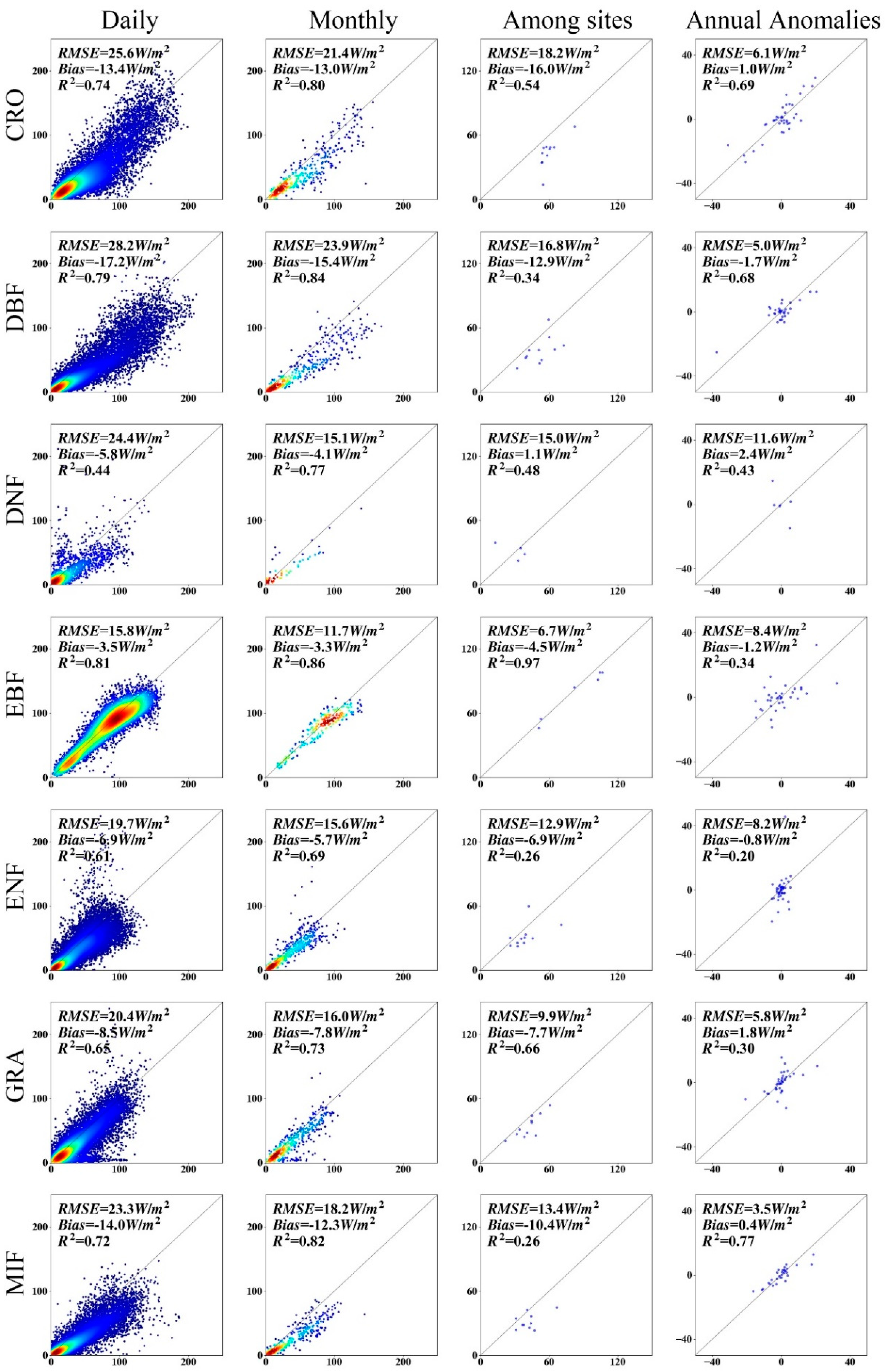
4.2. Model Validation and Comparison

The SPT model was validated using ten-fold cross-validation. Validations of the simulated and observed daily (monthly) ET at all sites illustrated the good performance of the SPT model for estimating seasonal ET variability (Figure 3). For different land-cover types, the performance of the SPT model differs greatly. The R2 of the estimated versus observed daily (monthly) ET ranged from 0.42 (0.58) (p < 0.01) at all SHR tower sites to 0.81 (0.86) (p < 0.01) at all EBF tower sites. The RMSE varied from 15.8 (11.7) W/m2 at all EBF tower sites to 28.2 (23.9) W/m2 at all DBF tower sites. Figure 3 also demonstrates the good ability of the SPT model for estimating the spatial variation. The RMSE of the site-averaged estimated ET varied from 6.7 W/m2 at all EBF tower sites to 18.2 W/m2 at all CRO tower sites, and R2 (99% confidence) varied from 0.22 at all SHR tower sites to 0.97 at all EBF tower sites. Overall, the SPT model accurately captured seasonal and spatial variations in ET. The SPT model also accurately yielded long-term variations in ET at all sites. The R2 (99% confidence) of the estimated and observed annual ET anomalies varied from 0.20 at all SHR tower sites and 0.77 at all MIF tower sites, and the largest RMSE was less than 12 W/m2 at all DNF tower sites, which was partially because of missing observed ET datasets caused by worse climatological conditions [18,46].
The estimated daily ET using the SPT model was also compared with those for the PT-JPL model. Table 3 shows the statistics (R2, RMSE and bias) of the comparison between the estimated and ground-observed daily ET from the first group of data using the second group of samples to calibrate the SPT model. For the forest EC sites, the RMSE for the estimated daily ET using the SPT model and PT-JPL model was 22.3 W/m2 and 31.2 W/m2, respectively. R2 of the estimated daily ET using the SPT model was higher than that for the PT-JPL model. For the crop, grass, and wetland sites, the SPT model had better performance than the PT-JPL model, with RMSEs less than 30 W/m2 and R2 values more than 0.85 (p < 0.01). For the SAW and SHR sites, the R2 of the estimated ET using the SPT model was much higher and the RMSE was less than 25 W/m2 compared with the PT-JPL model. Overall, the R2 for the SPT model increased by about 0.05 (p < 0.01) and the RMSE decreased by about 9 W/m2 at most forest flux tower sites. Similarly, the R2 for the SPT model increased by about 0.10 (p < 0.01) and the RMSE decreased by about 3 W/m2 at the CRO, GRA, WET, SAW, and SHR sites. This improvement over PT-JPL and other PT models is to calibrate the SPT model using ET ground measurements, with which the ground-measured ET was also used for validation. It is clear that the SPT model has better performance for estimating ET than that of the PT-JPL model. Therefore, compared with other PT models, the proposed SPT model has provided a better fit to EC observations.
The ET validation for each land-cover types agreed, in general, with results documented in the literature [30,34,49]. Ershadi et al. [30] evaluated four ET models using ground-measured ET from 20 FLUXNET tower sites and found that the best model is PT-JPL model with the RMSE of 66 W/m2. Vinukollu et al. [34] assessed three process-based ET models from 12 flux tower sites across the US and reported that these models yielded monthly ET with mean correlation of 0.54–0.57. Yebra et al. [49] compared estimates of ET produced with six different vegetation indices from the MODIS and three contrasting estimation approaches using ground-measured ET at 16 FLUXNET sites and documented that the PM-Gs (surface conductance) approach provided the lowest RMSE (average RMSE = 38 W/m2), and highest R2 (average R2 = 0.72). The validation accuracy of the estimated ET using the SPT model is higher than the above reported results.
To estimate the regional terrestrial ET, the parameters of Equation (4) were recalibrated based on ground-observed meteorological datasets and the MODIS NDVI datasets from all 100 EC flux tower sites. Table 4 demonstrates the Equation (4) coefficients for different land-cover types using a linear regression from MODIS NDVI, ground-observed Ta, Tmin, and RH. The SPT model is sufficiently representative to estimate regional ET due to the different terrestrial biomes and their locations of 100 EC sites.

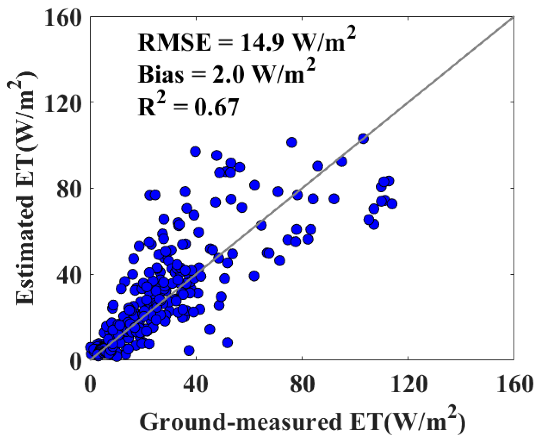
4.3. Model Application

4.3.1. Case I: Estimating Agricultural ET at High Spatial Resolution from Chinese GF-1 Data

The calibrated SPT model was applied to estimate agricultural ET of the Huailai region of China at high spatial resolution derived from GF-1 data during 2013–2017. Figure 4 illustrates the good correspondence between the estimated and ground-observed daily ET at the EC1 and EC2 sites. RMSE of estimated versus observed ET was 23.6 W/m2 and 24.4 W/m2, while that for the bias was −11.6 W/m2 and −1.2 W/m2. In addition, the R2 (99% confidence) was 0.84 and 0.81 at the EC1 and EC2 sites, respectively. These good results indicate that the ET estimation of the SPT model is reliable in the Huailai agricultural region of China.
Figure 5 shows the spatial distribution of the estimated daily ET of the Huailai agricultural region of China using the SPT model for three days in 2017. For DOY 133 (spring), the simulated ET using the SPT model was relatively lower than that for summer, with ET values from 0 to 50 W/m2. For DOY 190 (summer), the estimated ET achieved the maximum range of 0–130 W/m2, with the relatively highest ET values in crop and forest regions and the smallest values in urban regions in the middle part of the domain. For DOY 255 (fall), the estimated ET ranged from 0 to 80 W/m2, and the highest values occurred in the wetland regions of the top left part of the study area, which was consistent with the spatial patterns in the spring. Overall, the estimated ET tended towards high values during the period of summer because high vegetation coverage occurred in this region, while low ET values occurred in late fall after crops were harvested and other grass and forest declined. Few previous studies have focused on regional LE estimation at relatively high spatial resolutions using GF-1 data [46]. The SPT model successfully acquires finer spatial resolution ET using GF-1 NDVI data.

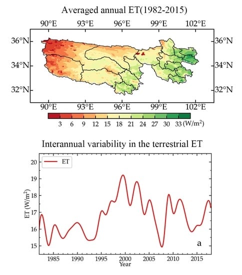
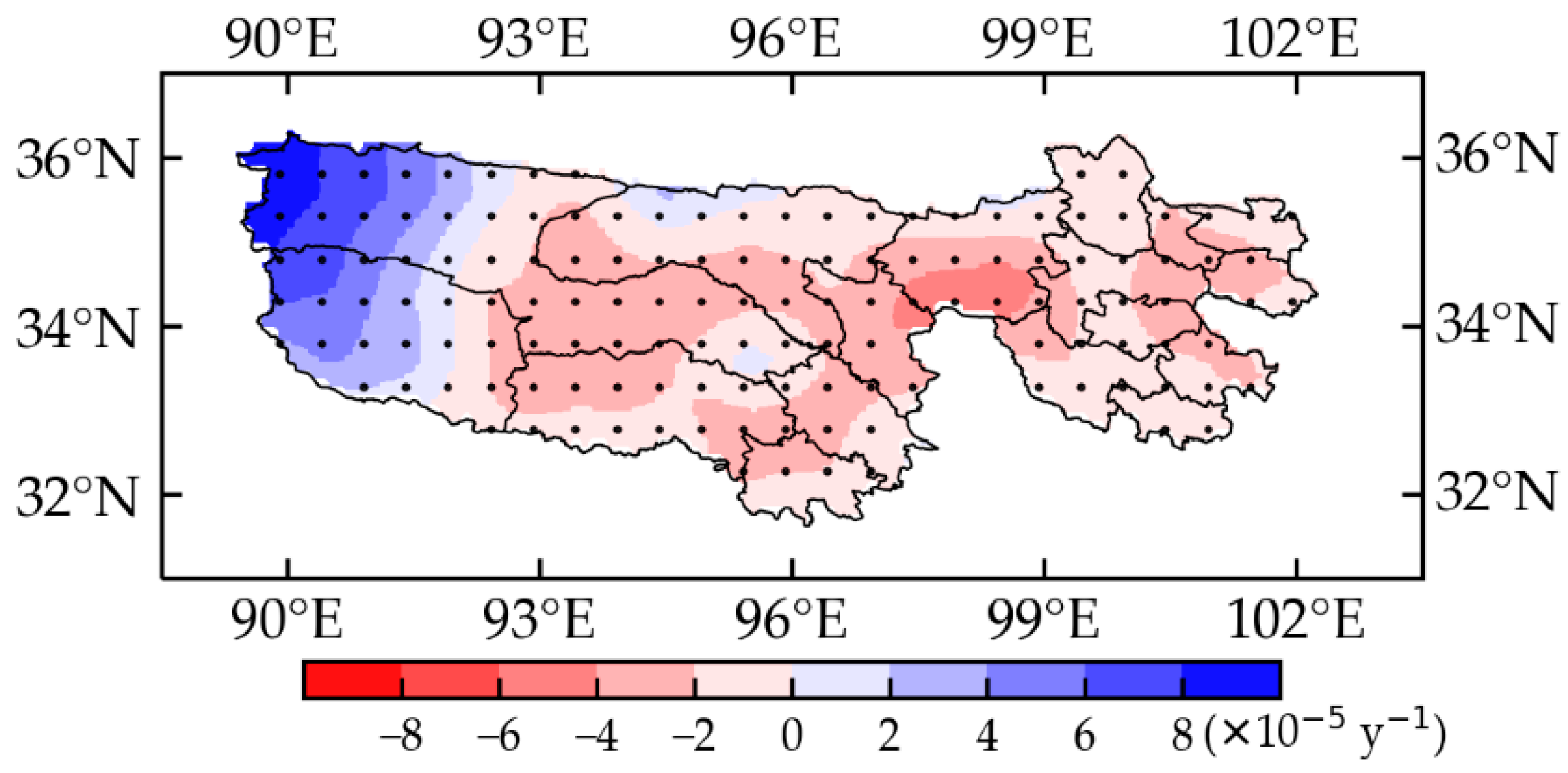
4.3.2. Case II: Monitoring Long-Term ET Variations in the Three-River Headwaters Region of China

The SPT model driven by CMFD meteorological data and GLASS NDVI products was also applied to generate the daily terrestrial ET of TRHR of China at a 0.05° spatial resolution between 1982 and 2018. This daily ET product was also validated based on ground-observed EC data collected from one TRH grass site. Figure 6 demonstrates the statistical comparison between the estimated and ground-observed ET at the TRH site. The R2 for the TRH site was approximately 0.67 at the 99% level of confidence, the bias was 2.0 W/m2 and the RMSE was 14.9 W/m2. The slightly positive bias may be caused by the limitations of the SPT model and the unclosed energy balance problem in EC data. However, Seguin et al. [50] pointed out that the ET estimation accuracy for application can be accepted as less than 50 W/m2. The accuracy of the results meets this basic requirement.
Figure 7 presents the spatial pattern of the multiyear (between 1982 and 2018) averaged annual ET in the TRHR. A large ET occurred in the eastern areas of the TRHR, while a small ET occurred across the western regions in the TRHR. The average annual ET of TRHR was 200 mm/year. Overall, the estimated annual ET anomalies of TRHR showed a significantly increasing trend of 0.3 W/m2 per decade (p < 0.05) from 1982–2018, and they coincided with widespread regional grass greening [51] (Figure 8). Regionally, the ET in the western areas of the TRHR accounted for more than 75% of the variation in the whole regional ET, and the positive annual ET in this region was mainly attributed to the regional vegetation (mainly grass) greening caused by global warning (0.065 °C/decade). The pattern of rising ET matched by an increasing NDVI indicated that increases in the NDVI (vegetation greening) represented the main contributor to the increasing ET trend over the western areas of the TRHR between 1982 and 2018. In contrast, the large-scale droughts characterized by the decreasing RH led to the regional ET decline in the eastern areas of the TRHR (Figure 9). More than 70% of the eastern region of the TRHR had positive correlations between annual ET and RH. The strong consistency of the patterns in terrestrial ET and RH trends illustrated that large-scale droughts were the main mechanism leading to the decreasing ET trend in the eastern areas of the TRHR from 1982–2018.

5. Discussion

5.1. Model Performance

Model validation at 100 global EC sites demonstrated that the proposed SPT model for estimating terrestrial ET was reliable across different terrestrial biomes. However, the SPT model had large differences in estimating ET across different land-cover types under the same environmental conditions. For example, the SPT model accounted for more than 75% of the ET variability for DBF, which may be associated with the strong seasonal variations in vegetation LAI in these biomes and the sensitivity of the NDVI to red reflectance and LAI changes [27,49,52]. In contrast, the SPT model only explained 50% of the ET variability for SHR and ENF because vegetation seasonal changes were weak and the NDVI yielded a poor performance for modeling vegetation transpiration [22,52,53]. This finding is consistent with previous studies documenting that the vegetation conductance of both ENF is half that of DBF [4,53]. In the SPT model, environmental factors, including Tmin, NDVI and RH, are considered to be the important regulators for downscaling the potential ET to actual ET. However, at the CRO, GRA, and SHR sites, Table 1 shows that the contribution of Tmin to f(c) is limited because the short vegetation is mainly controlled by water availability rather than Tmin [4,26]. Similarly, NDVI has no influence on f(c) at WET sites because the wetland is saturated with water [4,19]. The SPT model explains their differences using the same environmental factors with different calibration coefficients.
Although the SPT model only uses a simple linear formulation to parameterize f(c), it has lower errors in the inputs and has a better performance than that of the PT-JPL model. Importantly, the SPT model avoids Rn estimation directly using the Rs product as an important input and considers the differences in the f(c) calculation at different land-cover types, while the PT-JPL model ignores the classifications among land-cover types [10,27].
The simulation accuracy of the proposed model is affected by the errors in EC observations, the biases of forcing data, the scaling effects of different data and the structure of the model. Generally, EC observations have a bias of approximately 10–25% [54]; however, the EC technique is considered a good method to measure ET. Furthermore, EC suffers from energy imbalance problems because it does not capture large eddies, and the annual RBR for approximately 200 global FLUXNET sites is only 0.8 [55]. Although the fixed BR method was used to correct the ET, the uncertainty from EC observations remains indistinct [37,54]. Additionally, errors in meteorological variables (Tmin, Ta and RH) will also lead to errors in ET estimation. Recent studies have presented errors for CMFD datasets compared to ground observations [40,41,42]. Thus, the biases of meteorological data will reduce the accuracy of ET estimations.
Generally, the footprints of EC observations are less than 300 m [9]. However, the spatial resolutions of the MODIS (~1 km), GLASS (~5 km) and GF-1 (~16 m) NDVI products do not match the footprints of the EC observations. The mismatch among these datasets will cause large errors in the ET estimates. The structure of the SPT model also affects the ET simulation errors because the SPT model does not include SM and only uses RH to characterize moisture constraints, which may cause large uncertainties in ET estimation in semiarid and arid regions [16,22].

5.2. Implication for Regional Water Resources Assessment

Accurately quantifying the regional terrestrial ET is important for agricultural water resource management. Especially for agricultural regions, satellites with high spatial resolution (e.g., GF-1) have provided spatially and temporally frequent terrestrial observations for estimating field ET. Compared with LST, the NDVI changes slowly under a relatively short period to characterize SM conditions. However, the NDVI cannot reflect soil evaporation for bare soil [56]. Here, RH was used as a substitute for SM to estimate soil evaporation. Bouchet [57] reported a complementary theory that surface SM is associated with the atmospheric evaporation demand. Subsequently, Fisher et al. [10] developed a SM metric (RHVPD) to calculate soil evaporation. Similarly, Yan and Shugart [58] also found that RH is a better indicator than SM to estimate terrestrial ET, especially for late crop harvest periods. This good theoretical hypothesis illustrates the ability of the proposed SPT model to accurately estimate agricultural ET and has provided a usefully diagnostic assessment for field water consumption.
Monitoring long-term ET variations in ecologically fragile regions is critical for understanding regional hydrological dynamics and performing water resource assessments. In this study, the proposed SPT model has provided evidence for vegetation greening caused by global warming, which is important for controlling long-term ET variations in the TRHR of China. Previous studies have reported that climatic change (Ta and RH variations) has increased vegetation greening in northern high latitudes [59,60]. Similarly, the increase in ET is caused by the greening of vegetation, which is consistent with previous studies [2,61]. The results in this study also support this conclusion (Figure 8 and Figure 9). Other mechanisms that account for increasing ET seem to be less important due to the weak correlations between ET changes and other meteorological variables [62,63]. Further studies should highlight the combinations of satellite ET and ground measurements to investigate the impacts of human activities on hydrological processes.

6. Conclusions

A simplified Priestley–Taylor (SPT) ET model was developed to estimate global terrestrial ET across multiple biomes by combining incident shortwave radiation, a satellite vegetation index, and air relative humidity. The model coefficients of the environmental parameters are calibrated using the satellite-derived NDVI and ground-observed Ta, Tmin, RH, and ET. The proposed model was also validated based on a ten-fold cross-validation method across different plant function types using global FLUXNET observations from 100 global EC sites.
The validation results showed that the SPT model accurately captures seasonal and spatial variations in ET. For multiple biomes, the performance of the simplified PT model differed greatly. The R2 of the estimated versus observed daily (monthly) ET ranged from 0.42 (0.58) (p < 0.01) at all shrubland (SHR) flux tower sites to 0.81 (0.86) (p < 0.01) at all EBF flux tower sites. The RMSE of the site-averaged estimated ET varied from 6.7 W/m2 at all EBF flux tower sites to 18.2 W/m2 at all cropland (CRO) flux tower sites. The performance of the SPT model was good for simulating interannual ET variation, with an R2 of approximately 0.48 (p < 0.01). When compared with the PT-JPL model, the SPT model performed better at different regional scales. The SPT model was also applied to estimate agricultural ET at high spatial resolution from Chinese GF-1 data and to monitor long-term (1982–2018) ET variations in the TRHR of China. The SPT model presented here provides a bridge between EC flux data and regional applications.

Author Contributions

Conceptualization, Y.Y.; methodology, Z.D.; validation, X.Z.; formal analysis, R.Y. and Z.X. (Zhiqiang Xiao); investigation, X.G.; resources, K.J.; data curation, K.S., J.Y., and X.B.; writing—original draft preparation, Y.Y.; writing—review and editing, Y.Y., Z.D. and Z.X. (Zijing Xie) All authors have read and agreed to the published version of the manuscript.

Funding

This research was funded by the National Key Research Development Program of China (Grant No. 2016YFA0600103, Grant No. 2016YFB0501404 and Grant No. 2016YFA0600102), the Natural Science Fund of China (Grant No. 41671331 and Grant No. 41701483).

Institutional Review Board Statement

Not applicable.

Informed Consent Statement

Not applicable.

Data Availability Statement

Data available on request.

Acknowledgments

Authors would like to thank Ziwei Xu and Zhongli Zhu from Beijing Normal University, China, and Guirui Yu and Zhi Chen from Synthesis Research Center of Chinese Ecosystem Research Network, Key Laboratory of Ecosystem Network Observation and Modeling, Institute of Geographic Sciences and Natural Resources Research, Chinese Academy of Sciences, China, for providing ground-measured data. Acknowledgement for the data support from “National Earth System Science Data Center, National Science & Technology Infrastructure of China (http://www.geodata.cn accessed on 7 January 2021)”. MODIS LAI/FPAR, NDVI, albedo, and land-cover satellite products were obtained online (http://reverb.echo.nasa.gov/reverb accessed on 7 January 2021). The Chinese GF-1 WFV data was obtained from the Ministry of Ecology and Environmental Center for Satellite Application on Ecology and Environment (http://www.secmep.cn/ accessed on 7 January 2021). The authors thank Jie He and Kun Yang from the Institute of Tibetan Plateau Research, Chinese Academy of Sciences (http://westdc.westgis.ac.cn/ accessed on 7 January 2021) for providing the China Meteorological Forcing Dataset. This work used eddy covariance data acquired by the FLUXNET community and in particular by the following networks: AmeriFlux (US Department of Energy, Biological and Environmental Research, Terrestrial Carbon Program (DE-FG02-04ER63917 and DE-FG02-04ER63911)), AfriFlux, AsiaFlux, CarboAfrica, CarboEuropeIP, CarboItaly, CarboMont, ChinaFlux, Fluxnet-Canada (supported by CFCAS, NSERC, BIOCAP, Environment Canada, and NRCan), GreenGrass, KoFlux, LBA, NECC, OzFlux, TCOS-Siberia, USCCC. Authors acknowledge the financial support to the eddy covariance data harmonization provided by CarboEuropeIP, FAO-GTOS-TCO, iLEAPS, Max Planck Institute for Biogeochemistry, National Science Foundation, University of Tuscia, Université Laval, Environment Canada and US Department of Energy and the database development and technical support from Berkeley Water Center, Lawrence Berkeley National Laboratory, Microsoft Research eScience, Oak Ridge National Laboratory, University of California-Berkeley and the University of Virginia.

Conflicts of Interest

The authors declare no conflict of interest.

References

  1. Fisher, J.; Lee, B.; Purdy, A.; Halverson, G.; Dohlen, M.; Cawse-Nicholson, K.; Wang, A.; Anderson, R.; Aragon, B.; Arain, M.; et al. ECOSTRESS: NASA’s next generation mission to measure evapotranspiration from the International Space Station. Water Resour. Res. 2020, 56, e2019WR026058. [Google Scholar] [CrossRef]
  2. Jung, M.; Reichstein, M.; Ciais, P.; Seneviratne, S.I.; Sheffield, J.; Goulden, M.L.; Bonan, G.; Cescatti, A.; Chen, J.Q.; de Jeu, R.; et al. Recent decline in the global land evapotranspiration trend due to limited moisture supply. Nature 2010, 467, 951–954. [Google Scholar] [CrossRef] [PubMed]
  3. Song, L.S.; Liu, S.M.; Kustas, W.P.; Nieto, H.; Sun, L.; Xu, Z.W.; Skaggs, T.H.; Yang, Y.; Ma, M.G.; Xu, T.R.; et al. Monitoring and validating spatially and temporally continuous daily evaporation and transpiration at river basin scale. Remote Sens. Environ. 2018, 219, 72–88. [Google Scholar] [CrossRef]
  4. Wang, K.C.; Dickinson, R.E. A review of global terrestrial evapotranspiration: Observation, modeling, climatology, and climatic variability. Rev. Geophys. 2012, 50, RG2005. [Google Scholar] [CrossRef]
  5. Fisher, J.B.; Melton, F.; Middleton, E.; Hain, C.; Anderson, M.; Allen, R.; McCabe, M.F.; Hook, S.; Baldocchi, D.; Townsend, P.A.; et al. The future of evapotranspiration: Global requirements for ecosystem functioning, carbon and climate feedbacks, agricultural management, and water resources. Water Resour. Res. 2017, 53, 2618–2626. [Google Scholar] [CrossRef]
  6. Yao, Y.J.; Liang, S.L.; Li, X.L.; Chen, J.Q.; Liu, S.M.; Jia, K.; Zhang, X.T.; Xiao, Z.Q.; Fisher, J.B.; Mu, Q.Z.; et al. Improving global terrestrial evapotranspiration estimation using support vector machine by integrating three process-based algorithms. Agr. For. Meteorol. 2017, 242, 55–74. [Google Scholar] [CrossRef]
  7. Yao, Y.J.; Liang, S.L.; Cheng, J.; Liu, S.M.; Fisher, J.B.; Zhang, X.D.; Jia, K.; Zhao, X.; Qing, Q.M.; Zhao, B.; et al. MODIS-driven estimation of terrestrial latent heat flux in China based on a modified Priestley-Taylor algorithm. Agr. For. Meteorol. 2013, 171–172, 187–202. [Google Scholar] [CrossRef]
  8. Priestley, C.H.B.; Taylor, R.J. On the assessment of surface heat flux and evaporation using large scale parameters. Mon. Weather Rev. 1972, 100, 81–92. [Google Scholar] [CrossRef]
  9. Baldocchi, D.; Falge, E.; Gu, L.H.; Olson, R.; Hollinger, D.; Running, S.; Anthoni, P.; Bernhofer, C.; Davis, K.; Evans, R.; et al. FLUXNET: A new tool to study the temporal and spatial variability of ecosystem-scale carbon dioxide, water vapor, and energy flux densities. Bull. Am. Meteorol. Soc. 2001, 82, 2415–2434. [Google Scholar] [CrossRef]
  10. Fisher, J.B.; Tu, K.P.; Baldocchi, D.D. Global estimates of the land-atmosphere water flux based on monthly AVHRR and ISLSCP-II data, validated at 16 FLUXNET sites. Remote Sens. Environ. 2008, 112, 901–919. [Google Scholar] [CrossRef]
  11. Mu, Q.; Heinsch, F.A.; Zhao, M.; Running, S.W. Development of a global evapotranspiration algorithm based on MODIS and global meteorology data. Remote Sens. Environ. 2007, 111, 519–536. [Google Scholar] [CrossRef]
  12. Wang, K.C.; Liang, S.L. An improved method for estimating global evapotranspiration based on satellite determination of surface net radiation, vegetation index, temperature, and soil moisture. J. Hydrometeorol. 2008, 9, 712–727. [Google Scholar] [CrossRef]
  13. Allen, R.G.; Tasumi, M.; Morse, A.; Trezza, R.; Wright, J.L.; Bastiaanssen, W.; Kramber, W.; Lorite, I.; Robison, C.W. Satellite-based energy balance for mapping evapotranspiration with internalized calibration (METRIC)—Applications. J. Irrig. Drain. Eng. 2007, 133, 395–406. [Google Scholar] [CrossRef]
  14. Kalma, J.D.; McVicar, T.R.; McCabe, M.F. Estimating land surface evaporation: A review of methods using remotely sensed surface temperature data. Surv. Geophys. 2008, 29, 421–469. [Google Scholar] [CrossRef]
  15. Yao, Y.J.; Liang, S.L.; Li, X.L.; Zhang, Y.H.; Chen, J.Q.; Jia, K.; Zhang, X.T.; Fisher, J.B.; Wang, X.Y.; Zhang, L.L.; et al. Estimation of high-resolution terrestrial evapotranspiration from Landsat data using a simple Taylor skill fusion method. J. Hydrol. 2017, 553, 508–526. [Google Scholar] [CrossRef]
  16. Mu, Q.Z.; Zhao, M.S.; Running, S.W. Improvements to a MODIS global terrestrial evapotranspiration algorithm. Remote Sens. Environ. 2011, 115, 1781–1800. [Google Scholar] [CrossRef]
  17. Shan, N.; Zhang, Y.G.; Chen, J.M.; Ju, W.M.; Migliavacca, M.; Peñuelas, J.; Yang, X.; Zhang, Z.Y.; Nelson, J.A.; Goulas, Y. A model for estimating transpiration from remotely sensed solar-induced chlorophyll fluorescence. Remote Sens. Environ. 2021, 252, 112134. [Google Scholar] [CrossRef]
  18. Wang, K.C.; Dickinson, R.E.; Wild, M.; Liang, S.L. Evidence for decadal variation in global terrestrial evapotranspiration between 1982 and 2002: 1. Model development. J. Geophys. Res. Atmos. 2010, 115, D20112. [Google Scholar] [CrossRef] [Green Version]
  19. Yao, Y.J.; Liang, S.L.; Yu, J.; Chen, J.Q.; Liu, S.M.; Lin, Y.; Fisher, J.B.; McVicar, T.R.; Cheng, J.; Jia, K.; et al. A simple temperature domain two-source model for estimating agricultural field surface energy fluxes from Landsat images. J. Geophys. Res. Atmos. 2017, 122, 5211–5236. [Google Scholar] [CrossRef]
  20. Jackson, R.D.; Reginato, R.J.; Idso, S.B. Wheat canopy temperature: A practical tool for evaluating water requirements. Water Resour. Res. 1977, 13, 651–656. [Google Scholar] [CrossRef]
  21. Wang, K.C.; Wang, P.; Li, Z.Q.; Cribb, M.; Sparrow, M. A simple method to estimate actual evapotranspiration from a combination of net radiation, vegetation index, and temperature. J. Geophys. Res. Atmos. 2007, 112, D15107. [Google Scholar] [CrossRef]
  22. Yao, Y.J.; Zhang, Y.H.; Liu, Q.; Liu, S.M.; Jia, K.; Zhang, X.T.; Xu, Z.W.; Xu, T.R.; Chen, J.Q.; Fisher, J.B. Evaluation of a satellite-derived model parameterized by three soil moisture constraints to estimate terrestrial latent heat flux in the Heihe River basin of Northwest China. Sci. Total Environ. 2019, 695, 133787. [Google Scholar] [CrossRef] [PubMed]
  23. Anderson, M.C.; Norman, J.M.; Kustas, W.P.; Houborg, R.; Starks, P.J.; Agam, N. A thermal-based remote sensing technique for routine mapping of land-surface carbon, water and energy fluxes from field to regional scales. Remote Sens. Environ. 2008, 112, 4227–4241. [Google Scholar] [CrossRef]
  24. Kustas, W.P.; Norman, J.M. Evaluation of soil and vegetation heat flux predictions using a simple two-source model with radiometric temperatures for partial canopy cover. Agr. For. Meteorol. 1999, 94, 13–29. [Google Scholar] [CrossRef]
  25. Pablos, M.; Martínez-Fernández, J.; Piles, M.; Sánchez, N.; Vall-llossera, M.; Camps, A. multi-temporal evaluation of soil moisture and land surface temperature dynamics using in situ and satellite observations. Remote Sens. 2016, 8, 587. [Google Scholar] [CrossRef] [Green Version]
  26. Purdy, A.J.; Fisher, J.B.; Goulden, M.L.; Colliander, A.; Halverson, G.; Tu, K.; Famiglietti, J.S. SMAP soil moisture improves global evapotranspiration. Remote Sens. Environ. 2018, 219, 1–14. [Google Scholar] [CrossRef]
  27. Yao, Y.J.; Liang, S.L.; Li, X.L.; Chen, J.Q.; Wang, K.C.; Jia, K.; Cheng, J.; Jiang, B.; Fisher, J.B.; Mu, Q.Z.; et al. A satellite-based hybrid algorithm to determine the Priestley-Taylor parameter for global terrestrial latent heat flux estimation across multiple biomes. Remote Sens. Environ. 2015, 165, 216–233. [Google Scholar] [CrossRef] [Green Version]
  28. Pipunic, R.C.; Walker, J.P.; Western, A. Assimilation of remotely sensed data for improved latent and sensible heat flux prediction: A comparative synthetic study. Remote Sens. Environ. 2008, 112, 1295–1305. [Google Scholar] [CrossRef]
  29. Xu, T.R.; Liu, S.M.; Liang, S.L.; Qin, J. Improving predictions of water and heat fluxes by assimilating MODIS land surface temperature products into the Common Land Model. J. Hydrometeorol. 2011, 12, 227–244. [Google Scholar] [CrossRef]
  30. Ershadi, A.; McCabe, M.F.; Evans, J.P.; Chaney, N.W.; Wood, E.F. Multi-site evaluation of terrestrial evaporation models using FLUXNET data. Agr. For. Meteorol. 2014, 187, 46–61. [Google Scholar] [CrossRef]
  31. Jimenez, C.; Prigent, C.; Mueller, B.; Seneviratne, S.I.; McCabe, M.F.; Wood, E.F.; Rossow, W.B.; Balsamo, G.; Betts, A.K.; Dirmeyer, P.A.; et al. Global intercomparison of 12 land surface heat flux estimates. J. Geophys. Res. Atmos. 2011, 116, D02102. [Google Scholar] [CrossRef]
  32. Mueller, B.; Seneviratne, S.I.; Jimenez, C.; Corti, T.; Hirschi, M.; Balsamo, G.; Ciais, P.; Dirmeyer, P.; Fisher, J.B.; Guo, Z.; et al. Evaluation of global observations-based evapotranspiration datasets and IPCC AR4 simulations. Geophys. Res. Lett. 2011, 38, L06402. [Google Scholar] [CrossRef] [Green Version]
  33. Jin, Y.F.; Randerson, J.T.; Goulden, M.L. Continental-scale net radiation and evapotranspiration estimated using MODIS satellite observations. Remote Sens. Environ. 2011, 115, 2302–2319. [Google Scholar] [CrossRef] [Green Version]
  34. Vinukollu, R.K.; Wood, E.F.; Ferguson, C.R.; Fisher, J.B. Global estimates of evapotranspiration for climate studies using multi-sensor remote sensing data: Evaluation of three process-based approaches. Remote Sens. Environ. 2011, 115, 801–823. [Google Scholar] [CrossRef]
  35. Jiang, B.; Zhang, Y.; Liang, S.L.; Wohlfahrt, G.; Arain, A.; Cescatti, A.; Georgiadis, T.; Jia, K.; Kiely, G.; Lund, M.; et al. Empirical estimation of daytime net radiation from shortwave radiation and ancillary information. Agr. For. Meteorol. 2015, 211, 23–36. [Google Scholar] [CrossRef] [Green Version]
  36. Wang, K.C.; Liang, S.L. Estimation of daytime net radiation from shortwave radiation measurements and meteorological observations. J. Appl. Meteorol. Clim. 2009, 48, 634–643. [Google Scholar] [CrossRef]
  37. Twine, T.E.; Kustas, W.P.; Norman, J.M.; Cook, D.R.; Houser, P.R.; Meyers, T.P.; Prueger, J.H.; Starks, P.J.; Wesely, M.L. Correcting eddy-covariance flux underestimates over a grassland. Agr. For. Meteorol. 2000, 103, 279–300. [Google Scholar] [CrossRef] [Green Version]
  38. Jia, K.; Liang, S.L.; Gu, X.F.; Baret, F.; Wei, X.Q.; Wang, X.X.; Yao, Y.J.; Yang, L.Q.; Li, Y.W. Fractional vegetation cover estimation algorithm for Chinese GF-1 wide field view data. Remote Sens. Environ. 2016, 177, 184–191. [Google Scholar] [CrossRef]
  39. Xiao, Z.Q.; Liang, S.L.; Tian, X.D.; Jia, K.; Yao, Y.J.; Jiang, B. Reconstruction of long-term temporally continuous NDVI and surface reflectance from AVHRR data. IEEE J. Sel. Top. Appl. Earth Obs. Remote Sens. 2017, 10, 5551–5568. [Google Scholar] [CrossRef]
  40. Chen, Y.Y.; Yang, K.; He, J.; Qin, J.; Shi, J.C.; Du, J.Y.; He, Q. Improving land surface temperature modeling for dry land of China. J. Geophys. Res. Atmos. 2011, 116, D20104. [Google Scholar] [CrossRef]
  41. He, J.; Yang, K. China meteorological forcing dataset (1979–2015). Natl. Tibet. Plateau Data Cent. 2016. [Google Scholar] [CrossRef]
  42. Yang, K.; He, J.; Tang, W.J.; Qin, J.; Cheng, C.C.K. On downward shortwave and longwave radiations over high altitude regions: Observation and modeling in the Tibetan Plateau. Agr. For. Meteorol. 2010, 150, 38–46. [Google Scholar] [CrossRef]
  43. Zhang, K.; Kimball, J.S.; Nemani, R.R.; Running, S.W. A continuous satellite-derived global record of land surface evapotranspiration from 1983 to 2006. Water Resour. Res. 2010, 46, W09522. [Google Scholar] [CrossRef] [Green Version]
  44. Jung, M.; Reichstein, M.; Margolis, H.A.; Cescatti, A.; Richardson, A.D.; Arain, M.A.; Arneth, A.; Bernhofer, C.; Bonal, D.; Chen, J.; et al. Global patterns of land-atmosphere fluxes of carbon dioxide, latent heat, and sensible heat derived from eddy covariance, satellite, and meteorological observations. J. Geophys. Res. Atmos. 2011, 117, G00J07. [Google Scholar] [CrossRef] [Green Version]
  45. Petropoulos, G.; Sandric, I.; Hristopulos, D.; Carlson, T. Evaporative fluxes and surface soil moisture retrievals in a Mediterranean setting from Sentinel-3 and the “Simplified Triangle”. Remote Sens. 2020, 12, 3192. [Google Scholar] [CrossRef]
  46. Yao, Y.J.; Liang, S.L.; Fisher, J.B.; Zhang, Y.H.; Cheng, J.; Chen, J.Q.; Jia, K.; Zhang, X.T.; Bei, X.Y.; Shang, K.; et al. A novel NIR-Red spectral domain evapotranspiration model from the Chinese GF-1 satellite: Application to the Huailai agricultural region of China. IEEE Trans. Geosci. Remote Sens. 2021. [Google Scholar] [CrossRef]
  47. Arora, V. Modeling vegetation as a dynamic component in soil-vegetation-atmosphere transfer schemes and hydrological models. Rev. Geophys. 2002, 40, 1006. [Google Scholar] [CrossRef] [Green Version]
  48. Jarvis, P.G. The interpretation of the variations in leaf water potential and stomatal conductance found in canopies in the field. Philos. Trans. R. Soc. Lond. 1976, 273, 593–610. [Google Scholar]
  49. Yebra, M.; Van Dijk, A.; Leuning, R.; Huete, A.; Guerschman, J.P. Evaluation of optical remote sensing to estimate actual evapotranspiration and canopy conductance. Remote Sens. Environ. 2013, 129, 250–261. [Google Scholar] [CrossRef]
  50. Seguin, B.; Becker, F.; Phulpin, T.; Gu, X.F.; Guyot, G.; Kerr, Y.; King, C.; Lagouarde, J.P.; Ottlé, C.; Stoll, M.P.; et al. IRSUTE: A minisatellite project for land surface heat flux estimation from field to regional scale. Remote Sens. Environ. 1999, 68, 357–369. [Google Scholar] [CrossRef]
  51. Xu, G.; Zhang, H.; Chen, B.; Zhang, H.; Innes, J.; Wang, G.; Yan, J.; Zheng, Y.; Zhu, Z.; Myneni, R. Changes in vegetation growth dynamics and relations with climate over China’s landmass from 1982 to 2011. Remote Sens. 2014, 6, 3263–3283. [Google Scholar] [CrossRef] [Green Version]
  52. Huete, A.; Didan, K.; Miura, T.; Rodriguez, E.P.; Gao, X.; Ferreira, L.G. Overview of the radiometric and biophysical performance of the MODIS vegetation indices. Remote Sens. Environ. 2002, 83, 195–213. [Google Scholar] [CrossRef]
  53. Eugster, W.; Rouse, W.R.; Pielke, R.A.; McFadden, J.P.; Baldocchi, D.D.; Kittel, T.G.F.; Chapin, F.S.; Liston, G.E.; Vidale, P.L.; Vaganov, E.; et al. Land-atmosphere energy exchange in Arctic tundra and boreal forest: Available data and feedbacks to climate. Global Chang. Biol. 2000, 6, 84–115. [Google Scholar] [CrossRef]
  54. Foken, T. The energy balance closure problem: An overview. Ecol. Appl. 2008, 18, 1351–1367. [Google Scholar] [CrossRef]
  55. Wilson, K.; Goldstein, A.; Falge, E.; Aubinet, M.; Baldocchi, D.; Berbigier, P.; Bernhofer, C.; Ceulemans, R.; Dolman, H.; Field, C.; et al. Energy balance closure at FLUXNET sites. Agr. For. Meteorol. 2002, 113, 223–243. [Google Scholar] [CrossRef] [Green Version]
  56. Anderson, M.C.; Allen, R.G.; Morse, A.; Kustas, W.P. Use of Landsat thermal imagery in monitoring evapotranspiration and managing water resources. Remote Sens. Environ. 2012, 122, 50–65. [Google Scholar] [CrossRef]
  57. Bouchet, R. Evapotranspiration Reelle at Potentielle, Signification Climatique. Int. Assoc. Sci. Hydrol. Pub. 1963, 62, 134–142. [Google Scholar]
  58. Yan, H.; Shugart, H.H. An air relative-humidity-based evapotranspiration model from eddy covariance data. J. Geophys. Res. Atmos. 2010, 115, D16106. [Google Scholar] [CrossRef] [Green Version]
  59. Nemani, R.R.; Keeling, C.D.; Hashimoto, H.; Jolly, W.M.; Piper, S.C.; Tucker, C.J.; Myneni, R.B.; Running, S.W. Climate-driven increases in global terrestrial net primary production from 1982 to 1999. Science 2003, 300, 1560–1563. [Google Scholar] [CrossRef] [Green Version]
  60. Zhu, Z.C.; Piao, S.L.; Myneni, R.B.; Huang, M.T.; Zeng, Z.Z.; Canadell, J.G.; Ciais, P.; Sitch, S.; Friedlingstein, P.; Arneth, A.; et al. Greening of the Earth and its drivers. Nat. Clim. Chang. 2016, 6, 791–795. [Google Scholar] [CrossRef]
  61. Zeng, Z.Z.; Piao, S.L.; Li, L.Z.X.; Wang, T.; Ciais, P.; Lian, X.; Yang, Y.T.; Mao, J.F.; Shi, X.Y.; Myneni, R.B. Impact of earth greening on the terrestrial water cycle. J. Clim. 2018, 31, 2633–2650. [Google Scholar] [CrossRef]
  62. Yao, Y.J.; Liang, S.L.; Li, X.L.; Hong, Y.; Fisher, J.B.; Zhang, N.N.; Chen, J.Q.; Cheng, J.; Zhao, S.H.; Zhang, X.T.; et al. Bayesian multimodel estimation of global terrestrial latent heat flux from eddy covariance, meteorological, and satellite observations. J. Geophys. Res. Atmos. 2014, 119, 4521–4545. [Google Scholar] [CrossRef]
  63. Yao, Y.J.; Liang, S.L.; Cao, B.; Liu, S.M.; Yu, G.R.; Jia, K.; Zhang, X.T.; Zhang, Y.H.; Chen, J.Q.; Fisher, J.B. Satellite detection of water stress effects on terrestrial latent heat flux with MODIS shortwave infrared reflectance data. J. Geophys. Res. Atmos. 2018, 123, 11410–11430. [Google Scholar] [CrossRef] [Green Version]
Figure 1. Map of the 100 FLUXNET sites. CRO: cropland; GRA: grassland; DBF: deciduous broadleaf forest; MIF: mixed forest; DNF: deciduous needleleaf forest; SAW: savanna; EBF: evergreen broadleaf forest; SHR: shrubland; ENF: evergreen needleleaf forest; WET: wetland.
Remotesensing 13 00902 g001
Figure 2. Examples of case study areas and locations of the three flux towers. Huailai agricultural region and the Three-River Headwaters Region (TRHR) of China.
Remotesensing 13 00902 g002
Figure 3. Estimated terrestrial ET (y axis, W/m2) from the SPT model versus ground-observed ET (x axis, W/m2) for a series of cross-validation. CRO: cropland; GRA: grassland; DBF: deciduous broadleaf forest; MIF: mixed forest; DNF: deciduous needleleaf forest; SAW: savanna; EBF: evergreen broadleaf forest; SHR: shrubland; ENF: evergreen needleleaf forest; WET: wetland.
Remotesensing 13 00902 g003aRemotesensing 13 00902 g003b
Figure 4. Comparison of the observed and estimated daily ET based on the SPT model at the EC1 and EC2 sites.
Remotesensing 13 00902 g004
Figure 5. Spatial pattern of the estimated ET for different dates.
Remotesensing 13 00902 g005
Figure 6. Comparison of the observed and estimated daily ET based on the SPT model at the TRH site.
Remotesensing 13 00902 g006
Figure 7. Spatial pattern of multiyear (1982–2018) averaged annual ET of TRHR.
Remotesensing 13 00902 g007
Figure 8. (a) Interannual variability in the terrestrial ET and GLASS NDVI anomaly of the TRHR from 1982–2018. Spatial pattern of terrestrial (b) ET and (c) GLASS NDVI trends for 1982–2018 over the TRHR. The black solid dots stand for grids with 95% confidence.
Remotesensing 13 00902 g008
Figure 9. Spatial pattern of the RH trends for 1982–2018 over the TRHR. The black solid dots refer to grids with 95% confidence.
Remotesensing 13 00902 g009
Table 1. Correlation coefficients between the daily ET and daily Rs (rET, Rs), Tmin (rET, Tmin), NDVI (rET, NDVI), and RH (rET, RH). CRO: cropland; GRA: grassland; DBF: deciduous broadleaf forest; MIF: mixed forest; DNF: deciduous needleleaf forest; SAW: savanna; EBF: evergreen broadleaf forest; SHR: shrubland; ENF: evergreen needleleaf forest; WET: wetland.
Land-Cover TypesRET, RsRET, TminRET, NDVIRET, RH
CRO0.660.610.600.03
GRA0.490.510.500.04
WET0.730.530.480.01
SAW0.450.560.550.33
SHR0.540.410.400.09
DNF0.510.720.710.15
DBF0.750.730.670.05
ENF0.730.650.480.02
EBF0.570.620.450.07
MIF0.710.610.570.02
Table 2. Correlation coefficients (r) between the daily f(c) and daily Tmin (rfc, Tmin), NDVI (rfc, NDVI), and RH (rfc, RH). CRO: cropland; GRA: grassland; DBF: deciduous broadleaf forest; MIF: mixed forest; DNF: deciduous needleleaf forest; SAW: savanna; EBF: evergreen broadleaf forest; SHR: shrubland; ENF: evergreen needleleaf forest; WET: wetland.
Land-Cover TypesRfc, TminRfc, NDVIRfc, RH
CRO0.090.490.39
GRA0.060.520.51
WET0.340.040.41
SAW0.550.680.55
SHR0.090.450.44
DNF0.510.610.52
DBF0.570.540.33
ENF0.340.420.41
EBF0.410.350.33
MIF0.350.430.34
Table 3. Summary of a series of statistics (bias, RMSE, and R2) of the comparison between the ground-measured and estimated average daily ET using the two ET models of the first group. The second group samples were considered to be training datasets to calibrate coefficients of the proposed ET model. CRO: cropland; GRA: grassland; DBF: deciduous broadleaf forest; MIF: mixed forest; DNF: deciduous needleleaf forest; SAW: savanna; EBF: evergreen broadleaf forest; SHR: shrubland; ENF: evergreen needleleaf forest; WET: wetland.
Land-Cover TypesBias (W/m2)RMSE (W/m2)R2
PT-JPLSPTPT-JPLSPTPT-JPLSPT
CRO9.38.926.222.90.670.77
GRA6.35.616.413.80.710.77
WET8.878.517.214.10.690.80
SAW5.111.322.619.50.700.74
SHR12..111.120.618.80.670.68
DNF20.19.531.022.70.570.62
DBF22.120.133.725.60.720.77
ENF16.45.134.319.70.510.58
EBF20.47.838.824.70.510.61
MIF20.614.132.123.40.690.74
All15.613.833.323.80.600.71
Table 4. Coefficients (dimensionless) from global land-cover type-derived optimization of Equation (4) based on the MODIS NDVI data and ground-measured meteorology. CRO: cropland; GRA: grassland; DBF: deciduous broadleaf forest; MIF: mixed forest; DNF: deciduous needleleaf forest; SAW: savanna; EBF: evergreen broadleaf forest; SHR: shrubland; ENF: evergreen needleleaf forest; WET: wetland.
Land-Cover Typesα0α1α2α3
CRO−0.17360.00010.45320.5653
GRA−0.14930.00010.50260.4329
WET0.35030.00330.00010.1486
SAW−0.22120.00360.64730.3040
SHR−0.09920.00010.47250.3478
DNF−0.23580.00810.22570.7298
DBF−0.06040.00960.30060.3407
ENF−0.15660.00300.24460.5524
EBF−0.06050.00720.24120.3516
MIF−0.09170.00660.36700.3013
All−0.17600.00630.42190.4471
Publisher’s Note: MDPI stays neutral with regard to jurisdictional claims in published maps and institutional affiliations.

