
Risk Factor Detection and Landslide Susceptibility Mapping Using Geo-Detector and Random Forest Models: The 2018 Hokkaido Eastern Iburi Earthquake


Abstract
:
1. Introduction
2. Materials and Methods
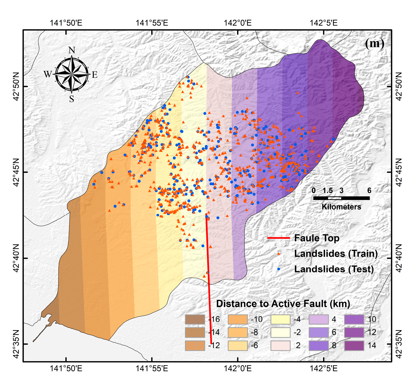
2.1. Study Area
2.2. Spatial Database
2.2.1. Landslide Inventory Map
2.2.2. Landslide Conditioning Factors
2.3. Methodology
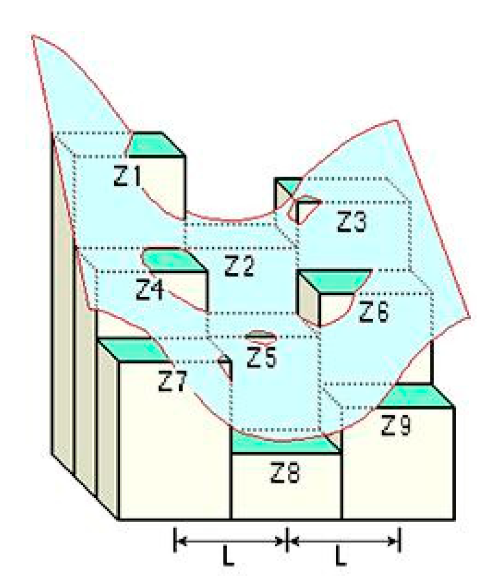
2.3.1. Geo-Detector
2.3.2. Dataset Generation Based on Geo-Detector
2.3.3. Random Forest Model
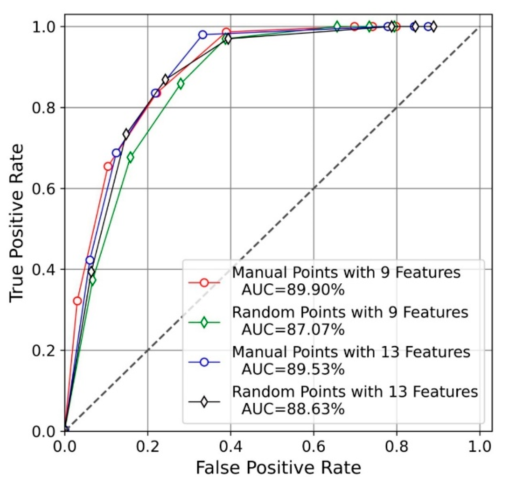
2.3.4. The Receiver Operating Characteristic Curve
3. Results
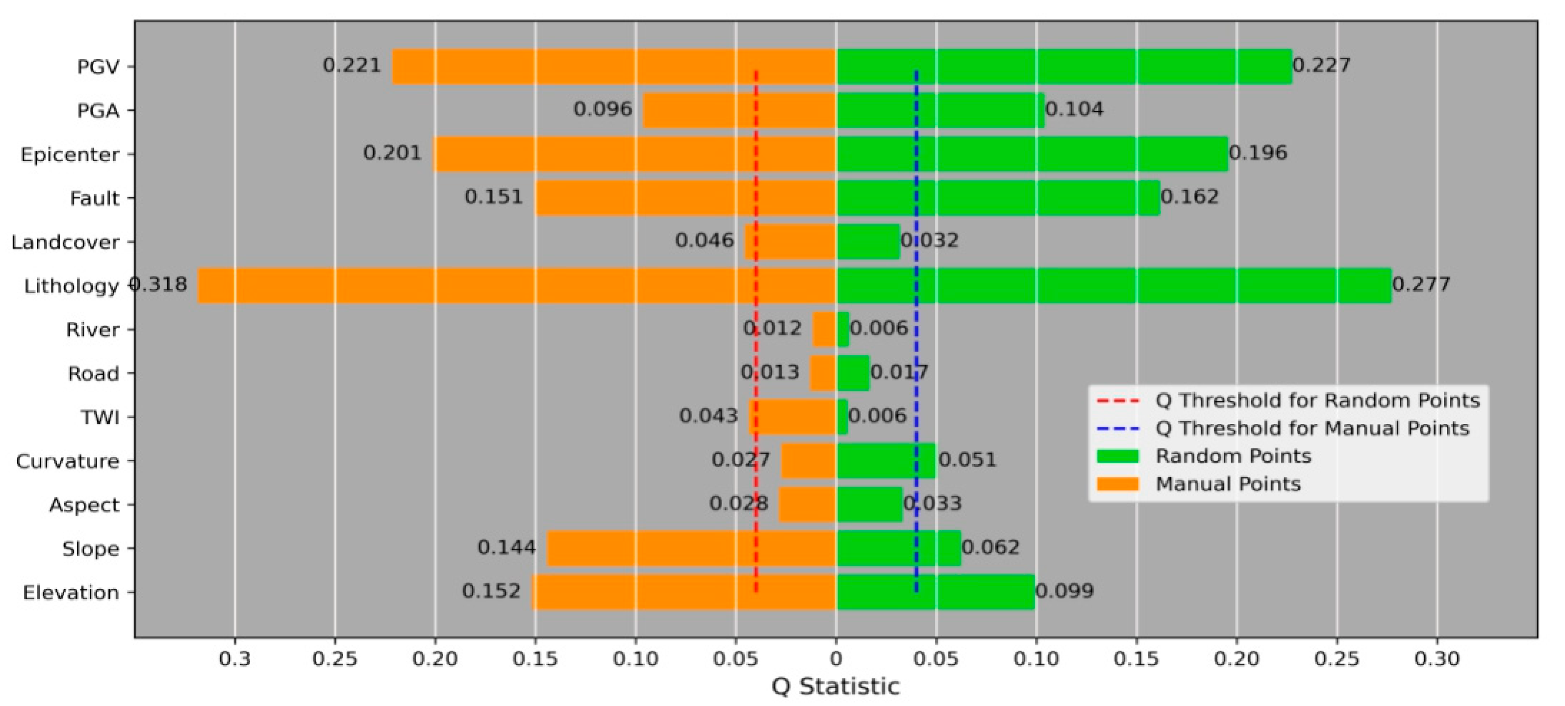
3.1. Geo-Detector and Dataset Generation
3.2. Model Accuracy Assessment and Comparison
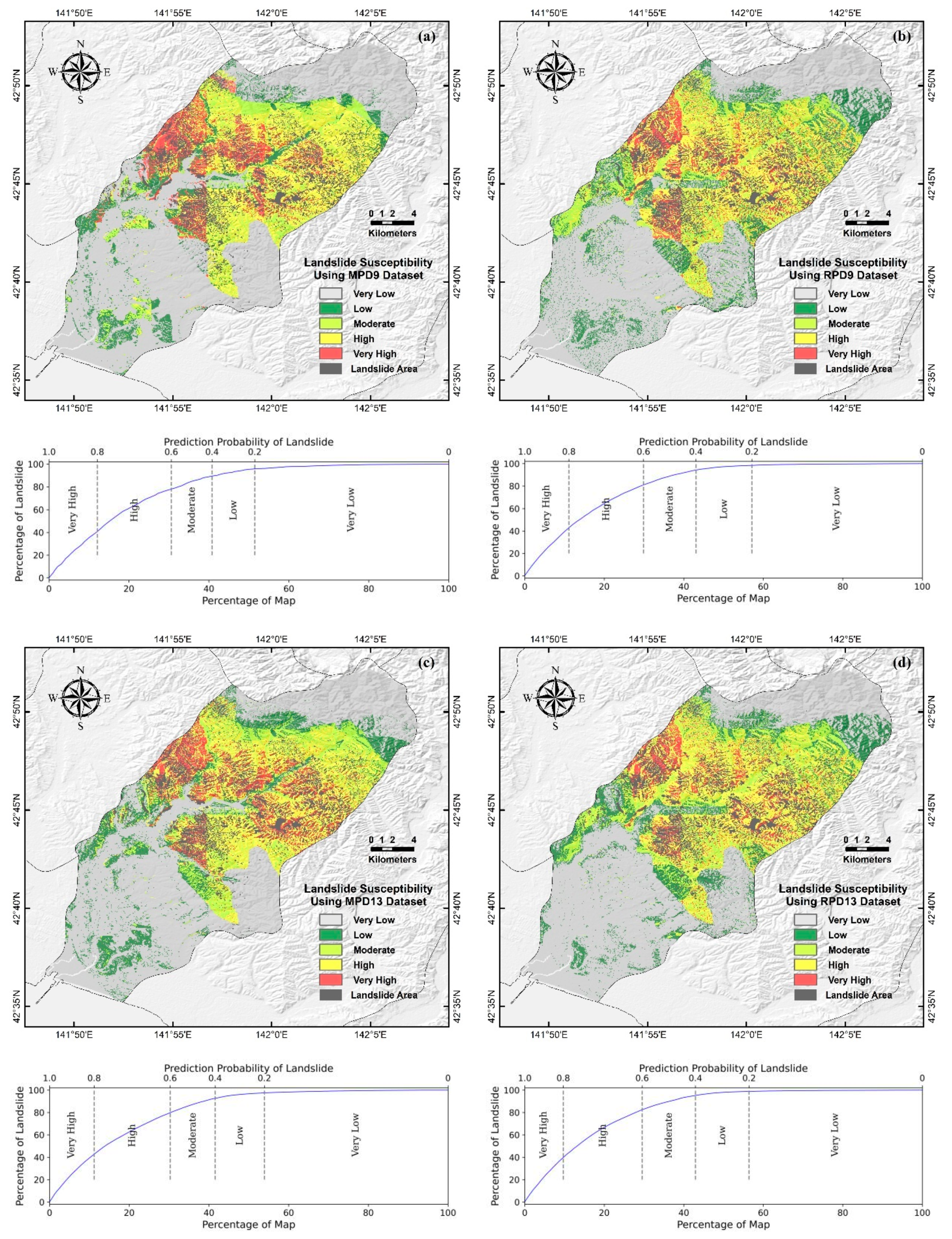
3.3. Landslide Susceptibility Mapping
4. Discussion
5. Conclusions
Author Contributions
Funding
Data Availability Statement
Acknowledgments
Conflicts of Interest
References
- Tien Bui, D.; Tuan, T.A.; Klempe, H.; Pradhan, B.; Revhaug, I. Spatial prediction models for shallow landslide hazards: A comparative assessment of the efficacy of support vector machines, artificial neural networks, kernel logistic regression, and logistic model tree. Landslides 2015, 13, 361–378. [Google Scholar] [CrossRef]
- Bălteanu, D.; Micu, M.; Jurchescu, M.; Malet, J.-P.; Sima, M.; Kucsicsa, G.; Dumitrică, C.; Petrea, D.; Mărgărint, M.C.; Bilaşco, Ş.; et al. National-scale landslide susceptibility map of Romania in a European methodological framework. Geomorphology 2020, 371. [Google Scholar] [CrossRef]
- Guzzetti, F.; Carrara, A.; Cardinali, M.; Reichenbach, P. Landslide hazard evaluation: A review of current techniques and their application in a multi-scale study, Central Italy. Geomorphology 1999, 31, 216. [Google Scholar] [CrossRef]
- Mărgărint, M.C.; Niculiţă, M. Landslide Type and Pattern in Moldavian Plateau, NE Romania. In Landform Dynamics and Evolution in Romania; Springer Geography; Springer: Cham, Switzerland, 2017; pp. 271–304. [Google Scholar] [CrossRef]
- Mărgărint, M.C.; Grozavu, A.; Patriche, C.V. Assessing the spatial variability of weights of landslide causal factors in different regions from Romania using logistic regression. Nat. Hazards Earth Syst. Sci. Discuss. 2013, 1, 1774. [Google Scholar] [CrossRef] [Green Version]
- Jebur, M.N.; Pradhan, B.; Tehrany, M.S. Optimization of landslide conditioning factors using very high-resolution airborne laser scanning (LiDAR) data at catchment scale. Remote Sens. Environ. 2014, 152, 150–165. [Google Scholar] [CrossRef]
- Reichenbach, P.; Rossi, M.; Malamud, B.D.; Mihir, M.; Guzzetti, F. A review of statistically-based landslide susceptibility models. Earth-Sci. Rev. 2018, 180, 60–91. [Google Scholar] [CrossRef]
- Luo, W.; Liu, C.-C. Innovative landslide susceptibility mapping supported by geomorphon and geographical detector methods. Landslides 2017, 15, 465–474. [Google Scholar] [CrossRef]
- van Westen, C.J.; Castellanos, E.; Kuriakose, S.L. Spatial data for landslide susceptibility, hazard, and vulnerability assessment: An overview. Eng. Geol. 2008, 102, 112–131. [Google Scholar] [CrossRef]
- Canli, E.; Thiebes, B.; Petschko, H.; Glade, T. Comparing physically-based and statistical landslide susceptibility model outputs—A case study from Lower Austria. In Proceedings of the EGU General Assembly 2015, Vienna, Austria, 12–17 April 2015. [Google Scholar]
- Pradhan, B.; Lee, S. Landslide susceptibility assessment and factor effect analysis: Backpropagation artificial neural networks and their comparison with frequency ratio and bivariate logistic regression modelling. Environ. Model. Softw. 2010, 25, 747–759. [Google Scholar] [CrossRef]
- Yang, J.; Song, C.; Yang, Y.; Xu, C.; Guo, F.; Xie, L. New method for landslide susceptibility mapping supported by spatial logistic regression and GeoDetector: A case study of Duwen Highway Basin, Sichuan Province, China. Geomorphology 2019, 324, 62–71. [Google Scholar] [CrossRef]
- Kavzoglu, T.; Sahin, E.K.; Colkesen, I. Landslide susceptibility mapping using GIS-based multi-criteria decision analysis, support vector machines, and logistic regression. Landslides 2013, 11, 425–439. [Google Scholar] [CrossRef]
- Yi, Y.; Zhang, Z.; Zhang, W.; Xu, Q.; Deng, C.; Li, Q. GIS-based earthquake-triggered-landslide susceptibility mapping with an integrated weighted index model in Jiuzhaigou region of Sichuan Province, China. Nat. Hazards Earth Syst. Sci. 2019, 19, 1973–1988. [Google Scholar] [CrossRef] [Green Version]
- Lee, S.; Pradhan, B. Landslide hazard mapping at Selangor, Malaysia using frequency ratio and logistic regression models. Landslides 2006, 4, 33–41. [Google Scholar] [CrossRef]
- Nefeslioglu, H.A.; Sezer, E.; Gokceoglu, C.; Bozkir, A.S.; Duman, T.Y. Assessment of Landslide Susceptibility by Decision Trees in the Metropolitan Area of Istanbul, Turkey. Math. Probl. Eng. 2010, 2010, 1–15. [Google Scholar] [CrossRef] [Green Version]
- Pradhan, B. A comparative study on the predictive ability of the decision tree, support vector machine and neuro-fuzzy models in landslide susceptibility mapping using GIS. Comput. Geosci. 2013, 51, 350–365. [Google Scholar] [CrossRef]
- Capecchi, V.; Perna, M.; Crisci, A. Statistical modelling of rainfall-induced shallow landsliding using static predictors and numerical weather predictions: Preliminary results. Nat. Hazards Earth Syst. Sci. 2015, 15, 75–95. [Google Scholar] [CrossRef]
- Fell, R.; Corominas, J.; Bonnard, C.; Leroi, E.; Cascini, L. Guidelines for landslide susceptibility, hazard and risk zoning for land use planning. Eng. Geol. 2008, 102, 83–84. [Google Scholar] [CrossRef] [Green Version]
- Guzzetti, F.; Ardizzone, F.; Cardinali, M.; Galli, M.; Reichenbach, P.; Rossi, M. Distribution of landslides in the Upper Tiber River basin, central Italy. Geomorphology 2008, 96, 105–122. [Google Scholar] [CrossRef]
- Donati, L.; Turrini, M.C. An objective method to rank the importance of the factors predisposing to landslides with the GIS methodology: Application to an area of the Apennines (Valnerina; Perugia, Italy). Eng. Geol. 2002, 63, 289. [Google Scholar] [CrossRef]
- Martínez-Álvarez, F.; Reyes, J.; Morales-Esteban, A.; Rubio-Escudero, C. Determining the best set of seismicity indicators to predict earthquakes. Two case studies: Chile and the Iberian Peninsula. Knowl.-Based Syst. 2013, 50, 198–210. [Google Scholar] [CrossRef]
- Fang, Z.; Wang, Y.; Peng, L.; Hong, H. Integration of convolutional neural network and conventional machine learning classifiers for landslide susceptibility mapping. Comput. Geosci. 2020, 139. [Google Scholar] [CrossRef]
- Jiménez-Perálvarez, J.D.; Irigaray, C.; El Hamdouni, R.; Chacón, J. Landslide-susceptibility mapping in a semi-arid mountain environment: An example from the southern slopes of Sierra Nevada (Granada, Spain). Bull. Eng. Geol. Environ. 2010, 70, 265–277. [Google Scholar] [CrossRef]
- Yamagishi, H.; Yamazaki, F. Landslides by the 2018 Hokkaido Iburi-Tobu Earthquake on September 6. Landslides 2018, 15, 2521–2524. [Google Scholar] [CrossRef] [Green Version]
- Shao, X.; Ma, S.; Xu, C.; Zhang, P.; Wen, B.; Tian, Y.; Zhou, Q.; Cui, Y. Planet Image-Based Inventorying and Machine Learning-Based Susceptibility Mapping for the Landslides Triggered by the 2018 Mw6.6 Tomakomai, Japan Earthquake. Remote Sens. 2019, 11, 978. [Google Scholar] [CrossRef] [Green Version]
- Moore, I.D.; Grayson, R.B.; Ladson, A.R. Digital terrain modelin—A review of hydrological, geomorphological, and biological applications. Hydrol. Process. 1991, 7, 18. [Google Scholar] [CrossRef]
- Zevenbergen, L.W.; Thorne, C.R. Quantitative Analysis of Land Surface Topography. Earth Surf. Process. Landf. 1987, 12, 56. [Google Scholar] [CrossRef]
- Quinn, P.F.; Beven, K.J.; Lamb, R. The in(a/tan/β) index: How to calculate it and how to use it within the topmodel framework. Hydrol. Process. 2010, 9, 22. [Google Scholar] [CrossRef]
- Falaschi, F.; Giacomelli, F.; Federici, P.R.; Puccinelli, A.; D’Amato Avanzi, G.; Pochini, A.; Ribolini, A. Logistic regression versus artificial neural networks: Landslide susceptibility evaluation in a sample area of the Serchio River valley, Italy. Nat. Hazards 2009, 50, 551–569. [Google Scholar] [CrossRef]
- Seamless Digital Geological Map of Japan. Available online: https://gbank.gsj.jp/seamless/index_en.html?p=download (accessed on 1 February 2021).
- Gong, P.; Liu, H.; Zhang, M.; Li, C.; Wang, J.; Huang, H.; Clinton, N.; Ji, L.; Li, W.; Bai, Y.; et al. Stable classification with limited sample: Transferring a 30-m resolution sample set collected in 2015 to mapping 10-m resolution global land cover in 2017. Sci. Bull. 2019, 64, 370–373. [Google Scholar] [CrossRef] [Green Version]
- Wang Jinfeng, X.C. Geo-detector: Principle and prospective. Acta Geogr. Sin. 2017, 72, 116–134. [Google Scholar] [CrossRef]
- Breiman, L.F.; Jerome, H.; Olshen, R.A.; Charles, J.C. Classification and Regression Trees; Wadsworth International Group: Wadsworth, OH, USA, 1984. [Google Scholar]
- Pedregosa, F.; Varoquaux, G.; Gramfort, A.; Michel, V.; Thirion, B.; Grisel, O.; Blondel, M.; Prettenhofer, P.; Weiss, R.; Dubourg, V.; et al. Scikit-learn: Machine Learning in Python. J. Mach. Learn. Res. 2011, 12, 2830. [Google Scholar]
- Breiman, L. Random forests. Mach. Learn. 2001, 45, 5–32. [Google Scholar] [CrossRef] [Green Version]
- Leo, B. Arcing Classifiers. Ann. Stat. 1999, 26, 801–849. [Google Scholar]
- Fawcett, T. An introduction to ROC analysis. Pattern Recognit. Lett. 2006, 27, 861–874. [Google Scholar] [CrossRef]
- Walter, S.D. Properties of the summary receiver operating characteristic (SROC) curve for diagnostic test data. Stat. Med. 2002, 21, 1237–1256. [Google Scholar] [CrossRef] [PubMed]
- Pradhan, B.; Lee, S. Regional landslide susceptibility analysis using back-propagation neural network model at Cameron Highland, Malaysia. Landslides 2009, 7, 13–30. [Google Scholar] [CrossRef]


| A | B | C | D | E | F | G | H | I |
|---|---|---|---|---|---|---|---|---|
| Datasets | Susceptibility | Pixels | Landslide Pixels | Density | Map Pixels | Percentage of Map | Map Landslide Pixels | Percentage of Landslide |
| (A) | (B) | (C) | (D) | (D/C) | (F) | (C/F) | (H) | (100D/H) |
| MPD9 | Very High | 54066 | 17339 | 0.32 | 574471 | 9.41 | 52190 | 33.22 |
| High | 132482 | 24693 | 0.19 | 574471 | 23.06 | 52190 | 47.31 | |
| Moderate | 55040 | 5476 | 0.10 | 574471 | 9.58 | 52190 | 10.49 | |
| Low | 52676 | 2599 | 0.05 | 574471 | 9.17 | 52190 | 4.98 | |
| Very Low | 280207 | 2083 | 0.01 | 574471 | 48.78 | 52190 | 3.99 | |
| RPD9 | Very High | 53832 | 19429 | 0.36 | 574471 | 9.37 | 52190 | 37.23 |
| High | 127100 | 24195 | 0.19 | 574471 | 22.12 | 52190 | 46.36 | |
| Moderate | 74226 | 6114 | 0.08 | 574471 | 12.92 | 52190 | 11.71 | |
| Low | 75861 | 1787 | 0.02 | 574471 | 13.21 | 52190 | 3.42 | |
| Very Low | 243452 | 665 | 0.00 | 574471 | 42.38 | 52190 | 1.27 | |
| MPD13 | Very High | 56965 | 20252 | 0.36 | 574471 | 9.92 | 52190 | 38.80 |
| High | 121146 | 22143 | 0.18 | 574471 | 21.09 | 52190 | 42.43 | |
| Moderate | 65411 | 6331 | 0.10 | 574471 | 11.39 | 52190 | 12.13 | |
| Low | 66750 | 2272 | 0.03 | 574471 | 11.62 | 52190 | 4.35 | |
| Very Low | 264199 | 1192 | 0.00 | 574471 | 45.99 | 52190 | 2.28 | |
| RPD13 | Very High | 47632 | 18392 | 0.39 | 574471 | 8.29 | 52190 | 35.24 |
| High | 131947 | 25964 | 0.20 | 574471 | 22.97 | 52190 | 49.75 | |
| Moderate | 73086 | 5671 | 0.08 | 574471 | 12.72 | 52190 | 10.87 | |
| Low | 71690 | 1608 | 0.02 | 574471 | 12.48 | 52190 | 3.08 | |
| Very Low | 250116 | 555 | 0.00 | 574471 | 43.54 | 52190 | 1.06 |
Publisher’s Note: MDPI stays neutral with regard to jurisdictional claims in published maps and institutional affiliations. |
© 2021 by the authors. Licensee MDPI, Basel, Switzerland. This article is an open access article distributed under the terms and conditions of the Creative Commons Attribution (CC BY) license (http://creativecommons.org/licenses/by/4.0/).
Share and Cite
Liu, Y.; Zhang, W.; Zhang, Z.; Xu, Q.; Li, W. Risk Factor Detection and Landslide Susceptibility Mapping Using Geo-Detector and Random Forest Models: The 2018 Hokkaido Eastern Iburi Earthquake. Remote Sens. 2021, 13, 1157. https://0-doi-org.brum.beds.ac.uk/10.3390/rs13061157
Liu Y, Zhang W, Zhang Z, Xu Q, Li W. Risk Factor Detection and Landslide Susceptibility Mapping Using Geo-Detector and Random Forest Models: The 2018 Hokkaido Eastern Iburi Earthquake. Remote Sensing. 2021; 13(6):1157. https://0-doi-org.brum.beds.ac.uk/10.3390/rs13061157
Chicago/Turabian StyleLiu, Yimo, Wanchang Zhang, Zhijie Zhang, Qiang Xu, and Weile Li. 2021. "Risk Factor Detection and Landslide Susceptibility Mapping Using Geo-Detector and Random Forest Models: The 2018 Hokkaido Eastern Iburi Earthquake" Remote Sensing 13, no. 6: 1157. https://0-doi-org.brum.beds.ac.uk/10.3390/rs13061157