1. Introduction
Cassava (
Manihot esculenta) is a South American crop that was first cultivated between 4000 and 2000 B.C. However, only recently has it become an important food source for the global population [
1]. It is estimated that over 278 million tons of cassava [
2] are cultivated annually, with its yield primarily serving as a source of carbohydrates for humans and secondarily as animal feed [
3]. The crop is grown in such high quantities due to its ability to thrive in marginally fertile soils and under various rainfall conditions [
4]. In addition to its hardy nature, cassava also tends to outperform many other tropical staple crops on a per hectare energy yield basis, leading to its widespread use across much of the tropics [
5,
6].
Considering the worldwide importance of cassava, especially within developing countries, yield improvements would help strengthen economic growth in these areas by shifting its cultivation from that of subsistence to a cash crop [
7]. Two areas in which cassava improvement is needed are early bulking (EB) of roots [
8,
9] and higher biomass of aboveground material [
10,
11]. Early bulking genotypes would have two significant advantages: a shortening of crop duration and increased yield [
12]. While cassava leaves are not the most widely consumed part of the plant, they nevertheless serve as an important vegetable in the Congo [
13], as well as an important animal feed for cattle and sheep, due to their high crude protein (~25%) content [
14].
Thus far, selection for both traits has only been achieved through costly destructive methods. Phenotyping of cassava is generally conducted by hand, which is a laborious and time-consuming task considering the size and long production cycle of the crop. As such, there is a need for a non-destructive method to quantify cassava root development and high-quality aboveground biomass. High-throughput phenotyping is one method that could speed up this process while also reducing costs [
15].
While it varies somewhat based upon genotype, the cassava physical structure essentially consists of broad leaves and open canopies, making for easy LiDAR returns [
16]. Additionally, the height of some genotypes can make it difficult to capture a full plant image with certain sensors [
17]; thus, a long-range, ground-based LiDAR unit would provide a reasonable capture of the full plant. Thankfully, there are a variety of scanners available on the market that can allow fast capture of 3D data. However, little, if any, literature exists on the use of this type of technique on cassava.
Terrestrial laser scanners (TLS) have the ability to record fine details of an object in 3D and often capture additional data such as intensity or RGB images. This is accomplished by emitting pulses of laser light (often at a single wavelength) at an object and using the time of flight and speed of light to determine the distance [
18]. The distance measure, along with the horizontal (azimuth) and vertical (zenith) angles between the instrument and the object, is recorded for each laser pulse. This information is used to perform simple trigonometric calculations to create a single point in 3D space which, when combined with other points, forms a point cloud. The point clouds from multiple scans captured around the object can be registered together and information related to the reflectance and pseudo-color [
19] images can be applied to form a data-dense 3D representation.
While no literature exists on its use for cassava, TLS has been used to assess phenotypic characteristics of many other crops, such as crop growth [
20], early stage plant detection [
21] and prediction of plant area [
22]. Aboveground biomass determination has been conducted in many species including oilseed rape (
Brassica napus), winter rye (
Secale cereale), winter wheat (
Triticum aestivum) and grasslands [
23,
24,
25]. Vineyard studies have also been conducted with significant results [
26].
In this study, we attempted to use a FARO Focus 120 TLS (FARO Technologies Inc., Lake Mary, FL, USA) to predict several categories of aboveground biomass in three genotypes of cassava, each of which differed in their aboveground structure. Our goal was to use TLS data to predict the biomass of the entire plant, as well as the biomass within specific height bins. Specifically, we tested several LiDAR data processing approaches to identify the best practices for using LiDAR data as a predictor of several measures of biomass (one of these approaches being the use of single scans versus two registered scans of each plant to correlate to the various biomass measures). Our results show that while binned height estimations did not provide good correlations, registered point clouds of the plants resulted in fair to excellent results based on genotype. Perhaps the most significant finding was that single, unregistered scans have comparable results to those of registered point clouds, drastically reducing the time needed to process data for this type of phenotyping.
2. Materials and Methods
2.1. Materials and Data Collection
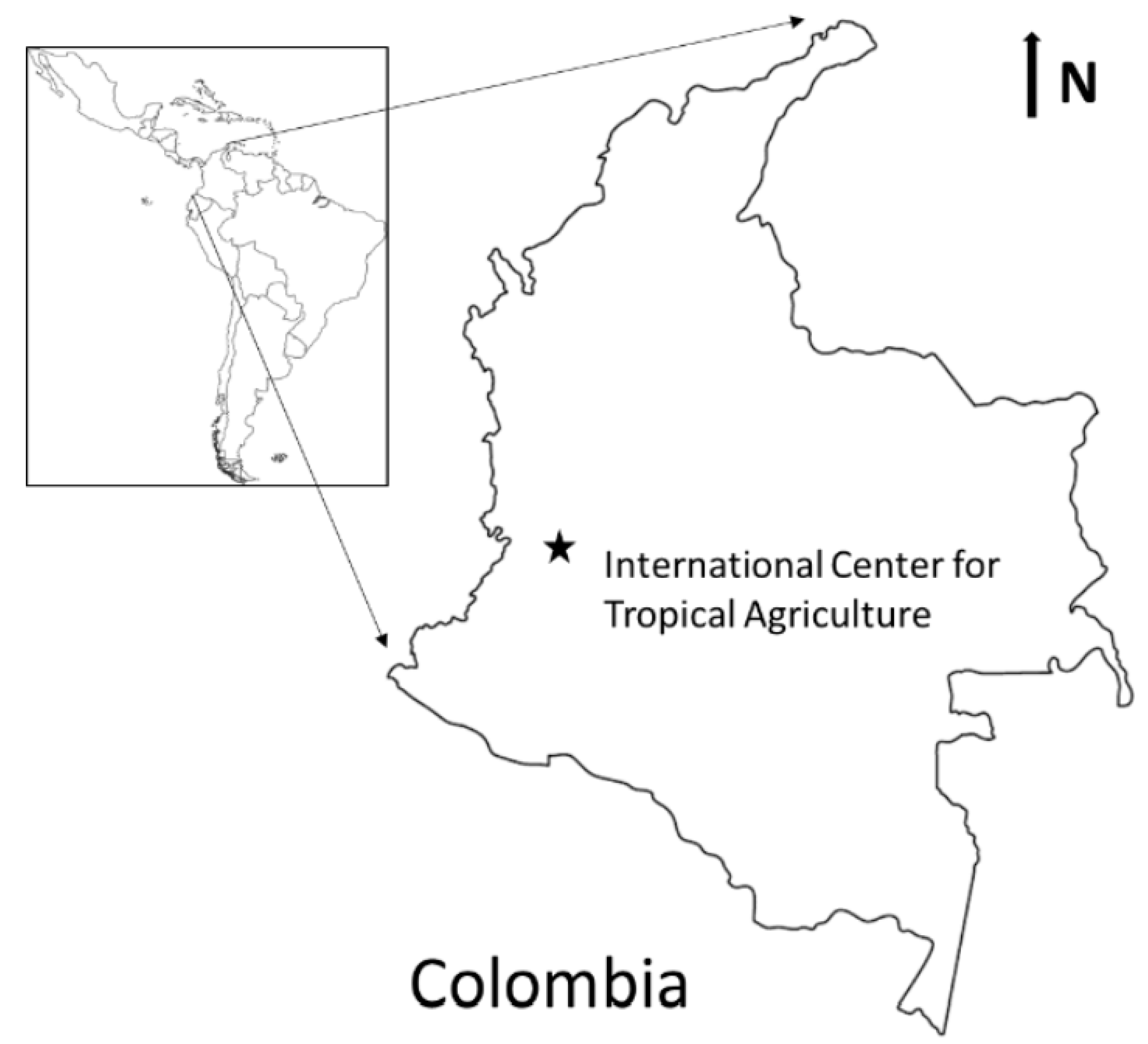
The experiment was conducted at the International Center for Tropical Agriculture (CIAT) in Palmira, Colombia (
Figure 1). Planting began in December of 2016, with subsequent plantings taking place approximately each month through August of 2017. The planting was carried out in a staggered fashion to allow data on all 9 age groups to be collected at one time (
Figure 2). This resulted in 9 age groups, from 3 to 11 months, during the data collection period in November of 2017.
Three genotypes of cassava were chosen based on their contrast in aboveground structure (
Figure 3). Genotype 1 (CM523-7) is a typical erect shrub-type cassava with few erect branches initiating above the ground surface. Genotype 2 (GM3893-65) is known as an asparagus type with its characteristic lack of branches and its leaves, which grow directly from the main stalk, allowing a higher planting density due to its very erect growth structure. Genotype 3 (HMC-1) is another shrub type, but it has a lower branching structure with branches often running near to the ground surface. Of both shrub types, Genotype 3 has a much lower growth pattern as compared to that of Genotype 1.
The age groups were created to produce variability in the biomass of each genotype. For each planting, 15 plants of each genotype were planted from cuttings into a 3 plant by 5 plant plot. The spacing between plants, as well as between rows, was 1 m. This exaggerated spacing was used to reduce the overlap between the plants. A double border was planted around the entire experiment, but no border was used between plots. The experiment received irrigation, fertilizer and any necessary pest treatments required to maintain normal growth. Data were captured on a subset of the plants in each plot. Within each plot, 3 to 5 plants were randomly selected, while the remaining were cut down and removed. This thinning was conducted to minimize the overlap between canopies in order to create space to get the FARO scanner in position.
Terrestrial laser scanning took place in mid-January 2017, using a FARO Focus 3D 120 terrestrial laser scanner. The Focus has a range of 0.6 to 120 m, with a ranging error of ±2 mm at 10 and 25 m, and operates at 905 nm. It is also equipped with a 70-megapixel color camera. The scanning was conducted at night to minimize the effect of wind on the point cloud quality as even a slight breeze can move the foliage, causing noise in the data. The scanning was conducted over a 3-night period and the winds during each night were recorded as negligible and caused only momentary movement of individual leaves.
Scanning took several nights due to the large number of scans needed for the study. The FARO scanner settings were set according to
Table 1. These settings were chosen as a tradeoff between scan quality and time required to capture data across the entire study. The scanner was mounted on an industrial tripod and was set to a height of approximately 1.25 m. The height varied between scans due to the exact placement of the legs in relation to the local topography. For each plant, a total of 2 scans were taken, one from the north and the other from the south side of the plant. The tripod-mounted scanner was placed in the adjacent row (approximately 1.5 m from the center of the target plant) and was aligned so the plant would fall roughly in the middle of the scanning window. No targets were placed in the scene to register the scans, as stumps of the removed plants and other objects provided sufficient references for registration. Only the points derived from the laser were used in the analysis, with no accompanying photographs.
Field data were harvested starting on the day after the first scan. These data included biomass, which was binned in 20-cm increments from the soil surface to the top of the plant. The binned data included two separate categories, one for the stalk and stem weights, and a second for the weight of the leaves. The bins were physically marked on each plant, using a large ruler and a number of small pieces of flagging tape to create a set of horizontal planes separating the bins. Prior to harvest, a large tarp was placed around the base of the plant to capture any dropped pieces. Harvesting was conducted manually by a team of CIAT employees. The harvest was carried out by first removing all the leaves from a plant and placing them in labeled paper bags for drying. Once all the leaves were removed, the stalks and stems were cut into manageable pieces and again placed in marked bags. The entire harvest took approximately 1 week to complete and another 3 weeks to dry the samples. To limit molding, a large walk-in cold storage was used to store the samples prior to their time in the dryer. All bags were dried in commercial drying ovens at 70 °C and were weighed to capture dry weight.
2.2. Data Processing
Plants used for the analysis were randomly selected from the pool by genotype, which resulted in 18 plants per genotype for a grand total of 54 across the 3 genotypes. For each plant, the two scans were registered together in FARO SCENE software using common points available in the environment (
Figure 4). The target points used were mainly the stalks of the previously removed plants along with some field markers and other objects in the scene. Once registration was complete, each plant’s point cloud was roughly clipped to remove unnecessary background points and was then exported as a .xyz file. The .xyz format was chosen to facilitate analysis in CloudCompare 2.10 beta (CC) [
27], an open source point cloud editing and analysis program.
In addition, the unregistered scans (2 per plant) were also roughly clipped and exported as .xyz files to allow single-scan analysis. The single scans were used to assess the potential to correlate to the field biomass measures without the need for the registration step. While targets can be used to automate the registration process, this is not always feasible nor reliable, and therefore manual adjustments may still be needed. Thus, manual registration, through point picking of common points via various software packages, is often the method used. Our group wanted to assess the potential of bypassing the registration step by using a single scan per plant for the analysis.
The following processing steps were applied to the registered scans as well as the single scans: Each point cloud was opened in CC where it was further clipped to remove all points which were not plant points or ground points which fell below the plant. All the ground points below the plant were kept in order to facilitate the segmentation of the ground from the plant points. In addition, the Statistical Outlier Removal (SOR) filter was run to help remove outliers in each point cloud. The SOR values used were determined through trial and error using visual assessment (
Table 2). Each file was then exported in the .las format to allow analysis in R-3.6.1 (GNU Project), a statistical computing and graphics programming language.
2.3. Ground Classification
R-Studio Desktop, an integrated development environment for the programming language, was used to visualize the code utilized for the analysis. In R, the lidR package was used to run lasground_pmf (Progressive Morphological Filter, or PMF). The lidR package is a collection of code and functions that allow users to analyze data in .las and .laz formats, which are commonly used for storing LiDAR data. The lasground_pmf function uses a filter to segment ground points for each point cloud so that vegetation can be separated from ground points for analysis.
The two variables for the filter are: (1) the sequence of window size(s) to be used in filtering the ground returns and (2) the sequence of threshold height(s) above the ground surface to be considered as a ground return [
28]. For this analysis, trial and error was used to determine PMF settings (
Table 3).
2.4. Binning
The point cloud had to be binned by height to match the field data. All ground points except for those directly below the main stalk were clipped manually in CC. These point clouds were then loaded back into R and the average height of the few remaining ground points was determined. The point cloud data were binned using the average ground height as a reference and then simply segmenting the data by height to match the field data.
2.5. Subsampling
We tested the effect of point cloud density on the ability of the point count to predict total plant dry weight. To do this, the additional preprocessing step of subsampling the point cloud using the subsampling tool in CC was completed. The minimum space between points was set to 0.002 m (2 mm), as it closely resembles the theoretical maximum ranging accuracy of the FARO Focus 120 (±0.02 mm @ 10 m) and would not degrade the data.
2.6. Data Analysis
All regressions were completed in R using the base function lm (linear model) and all outputs were generated using the package ggplot2. In addition, all bootstrap analyses were conducted using the boot package in R. Bootstrapping is a resampling technique which allows estimation of the population response and associated uncertainty to a variable through sampling with replacement. For details on bootstrapping, see Efron and Tibshirani, 1994 [
29]. We used the bias-corrected and accelerated bootstrap (BCa) method as it has the ability to correct for bias and skewness in the distribution of the output estimates. The number of iterations used was 5000 with a confidence level of 0.95. All bootstrap analyses used in this study were conducted using the same method. To test the ability of the FARO to predict cassava biomass within different height bins, we regressed the binned point cloud data against the binned field data for all 54 plants. The number of points in each point cloud height bin was regressed against the total dry plant weight (stalk and stem + leaf wts.) and the leaf-only dry weight. A bootstrap analysis was also conducted for both.
Our group examined the relationship between the LiDAR data and the entire plant dry weight. This was conducted for the registered-only, the registered and subsampled and the single-scan subsampled LiDAR datasets. For the single-scan analysis, the selection of which scan (north or south) to use was conducted through random selection on a plant-by-plant basis. For each of the three analyses, the point count of each plant’s entire point cloud was regressed against the total plant dry weight (e.g., a dry weight of 1333 g to a point count of 332,249). In addition, a bootstrap analysis was also conducted.
Our group also tested the relationship between the LiDAR data and the leaf-only dry weight. This was conducted for the registered and subsampled and the single-scan subset LiDAR datasets. For each of these analyses, the point count of each plant’s entire point cloud was regressed against the plant’s leaf dry weight. A bootstrap analysis was conducted for each. A by-genotype analysis using the leaf dry weight was conducted for both the registered and subsampled and the single-scan subsampled datasets. This was conducted by subsetting the dataset by genotype and then running the same analysis as mentioned above.
The average ratio of leaf to stalk and stem weight for each genotype was determined. This was conducted by taking the leaf weight for each plant and dividing it by the stalk and stem weight. These ratio values for each plant were then averaged across the genotype. In addition, a shape analysis was conducted to assess the variation in the squareness of the horizontal growth in the X and Y directions for Genotypes 1 and 3. This analysis was conducted by using the dimensions of the bounding box for each plant in CC. These two dimensions were captured for each plant in the two genotypes and were then turned into a ratio by dividing the two dimensions. The closer the value was to 1.00, the squarer the plant’s horizontal growth. A test of equal variance was conducted in R, which found the variances were not equal. A t-test using unequal variances was conducted in R to test if the squareness ratios derived from Genotypes 1 and 3 were equal data.
3. Results
3.1. Binned Height
Binned aboveground biomass data were correlated to the binned LiDAR data. Both the total plant dry weight and the leaf-only dry weights were tested. Using the total plant dry weight, we achieved an R
2 of 0.01 with a
p-value of 0.02 (data not shown). A slight improvement was seen using only the leaf dry weights, where we found an R
2 of 0.19 at a
p-value of 6.62 × 10
−9 (
Figure 5). The bootstrap analysis suggested an R
2 of 0.19, with a bias of 4.03 × 10
−3 and an STDEV of 0.06. The 95% R
2 confidence intervals for the bootstrap analysis were 0.08 to 0.31.
3.2. All Genotypes Combined
For the registered point clouds, the total LiDAR point count for each plant was regressed against the entire plant dry weight. The linear regression resulted in an R2 value of 0.45 and a p-Value of 1.73 × 10⁻⁸ (data not shown). The bootstrapping resulted in a mean R2 value of 0.46, a bias of 0.02 and standard error of 0.13. The 95% confidence ranged from 0.21 to 0.7.
To improve the correlation, we took the additional step to subsample each registered point cloud in an attempt to standardize its spatial density. The subsampling improved the correlation, with an R
2 value of 0.73 and a
p-value of 1.26 × 10
−16 (
Figure 6). The bootstrap analysis resulted in a mean R
2 of 0.74, a bias of 5.79 × 10
−4 and a standard error of 0.07 with a 95% confidence between 0.55 and 0.84.
A major limitation to the use of TLS data, and LiDAR data in general, is the time-consuming process of registration. We tested the potential of the point count from a single scan, which was subsampled, to correlate to the entire plant dry weight. The correlation was similar to that obtained via the registered and subsampled clouds. The R
2 value of the regression was 0.73 with a
p-value of 2.2 × 10
−16 (
Figure 7). The bootstrap analysis had a mean R
2 of 0.74, a bias of 8.23 × 10
−4 and an STDEV of 0.07. The 95% confidence interval was 0.57 to 0.84.
3.3. By Genotype
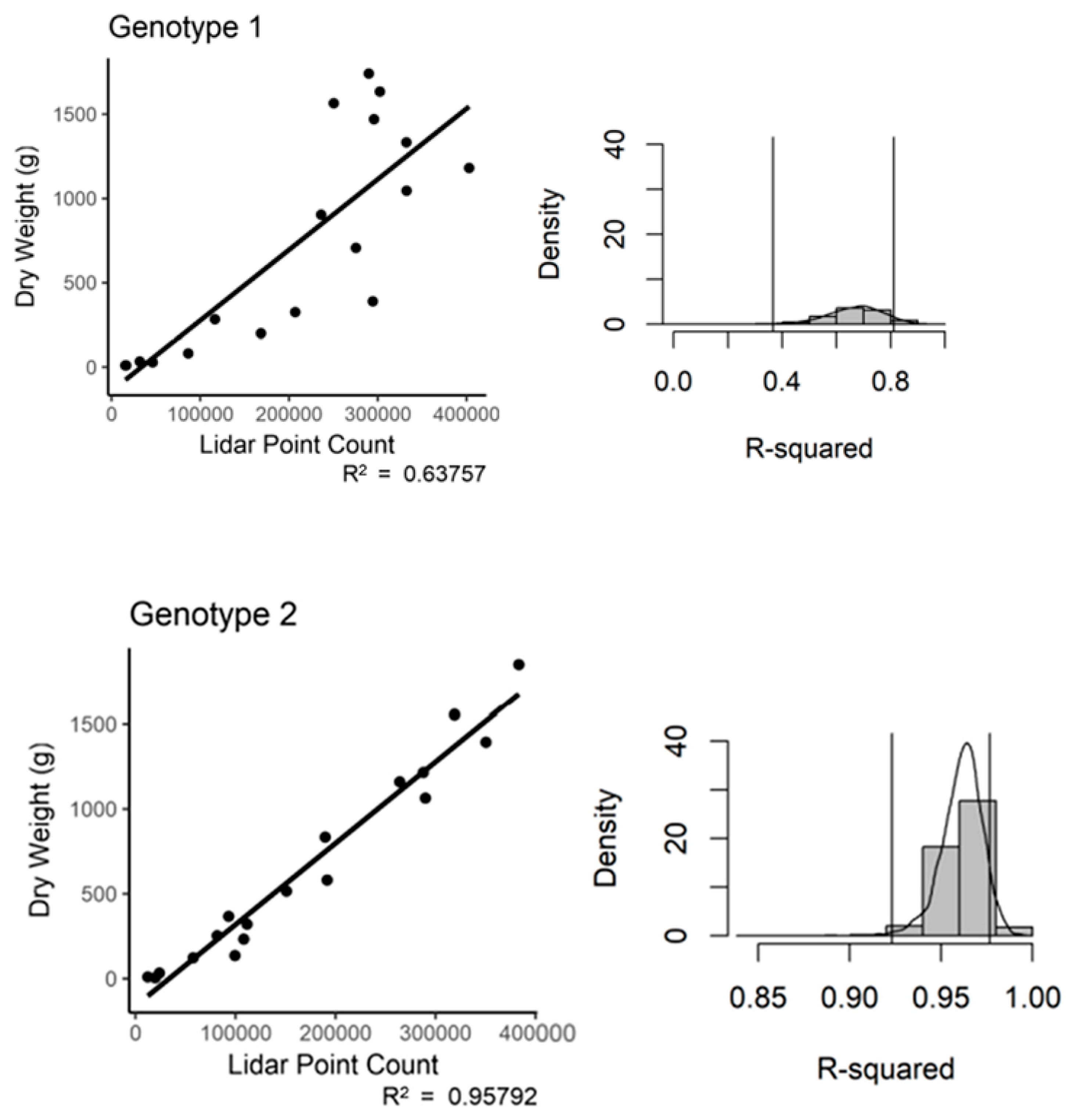
The study included three different genotypes of cassava, which contrasted in their aboveground structure. We tested the ability of the TLS technology to predict plant biomass between the various structural types of cassava. When we assessed the registered and subsampled data on a genotype basis, we found variation in the predictive power of the LiDAR technology (
Figure 8). Note that the bootstrap density scale was adjusted to allow full representation of the trend line. Genotype 1 had an R
2 of 0.64 and a
p-value of 4.32 × 10
−5. Genotype 2 performed well with an R
2 of 0.95 and a
p-value of 1.12 × 10
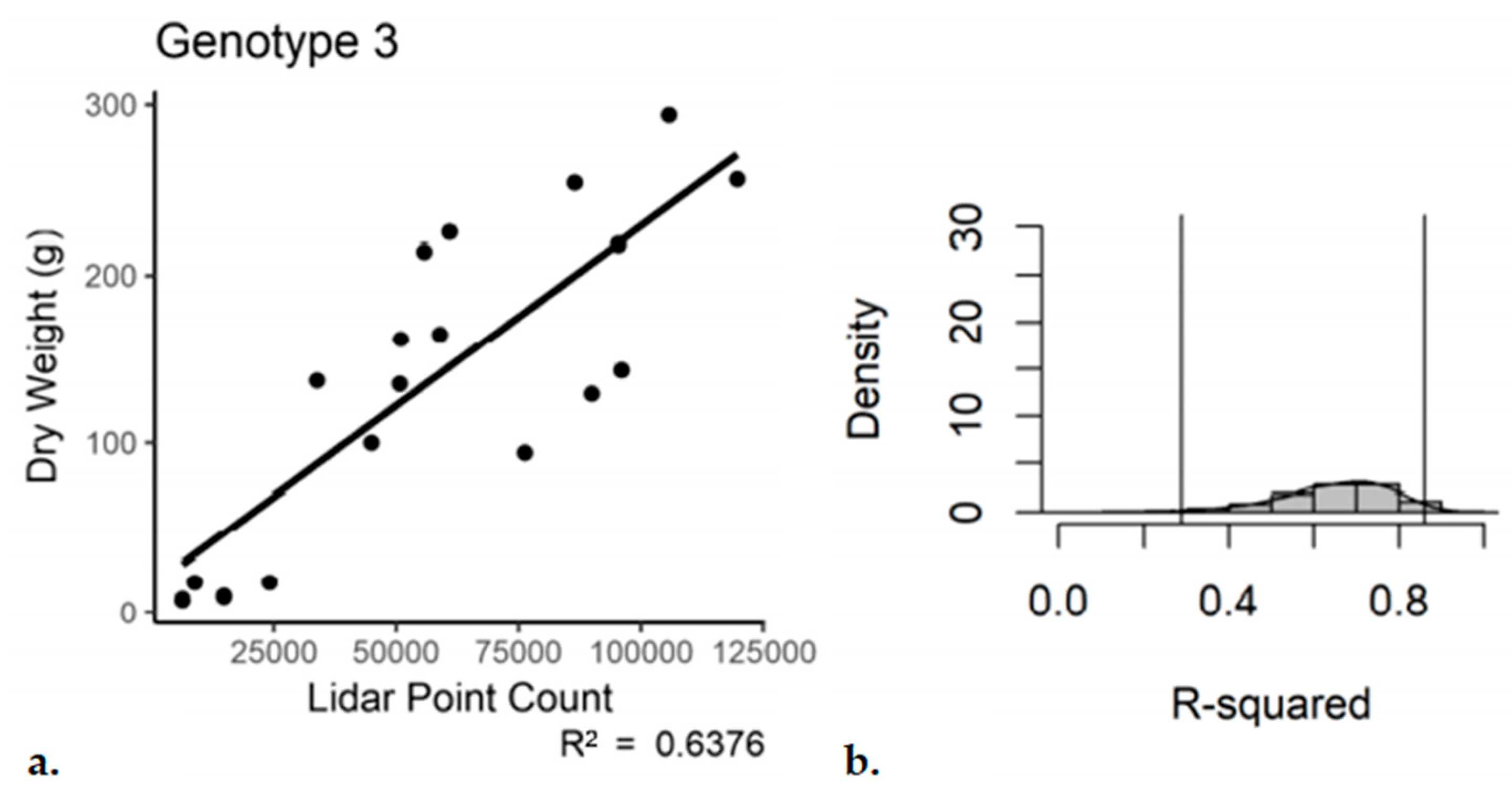
−12. Genotype 3 fell in the middle with an R
2 of 0.71 and a
p-value of 6.45 × 10
−6. The bootstrap results suggest a large amount of variation in the predictive power for both Genotypes 1 and 3 (
Table 4).
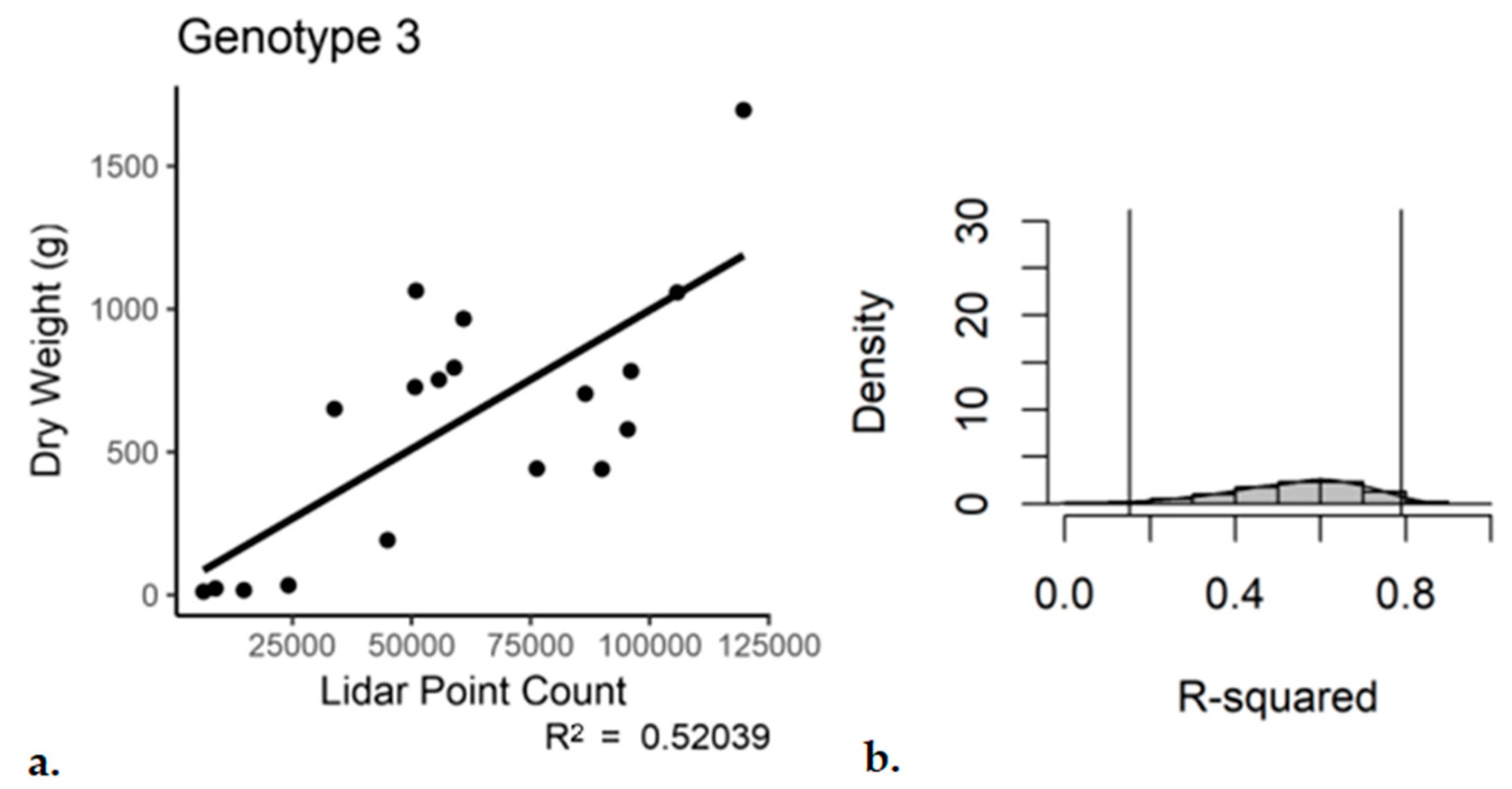
The same by-genotype analysis was conducted for the single scan with subsampling dataset. Genotypes 1 and 2 performed similar to the registered and subsampled dataset (
Table 5 and
Table 6). However, for Genotype 3, the outcome was not as good. For the third genotype, the use of a single scan with subsampling resulted in an R
2 of 0.52 with a
p-value of 4.38 × 10
−4 (
Figure 9). The bootstrap analysis told a similar story, with a notable increase in the range of the 95% confidence interval for Genotype 3 (0.15–0.79).
3.4. Leaf Dry Weight
Our group questioned if variations in the stem weights were causing the change in predictive power of the technology between genotypes. In order to test this, we regressed against only the leaf dry weights for both the registered and subsampled and single-scan subsampled datasets.
The first analysis looked at the effect across all genotypes. The registered and subsampled dataset resulted in the best R
2 value of 0.8 with a
p-value of 2 × 10
−16 (
Figure 10). The bootstrap results suggested a 95% confidence interval for the R
2 between 0.63 and 0.88, which again were the best across the study. The single-scan subsampled dataset did not perform quite as well with an R
2 of 0.78 (
Table 5).
Using the leaf dry weight on a by-genotype basis for the registered and subsampled dataset resulted in a similar response for Genotypes 1 and 2, as with using the entire plant dry weight (
Table 5 and
Table 6). However, Genotype 3 had an improved R
2 of 0.83 with a
p-value of 1.13 × 10
−7 (
Figure 11).
We analyzed the single-scan subsampled dataset against the leaf dry weights on a by-genotype basis. Interestingly, we found a similar pattern as with the same dataset regressed against the entire plant dry weight. Genotypes 1 and 2 performed about the same (
Table 5 and
Table 6), while Genotype 3 again performed poorly, albeit with a slight improvement over the entire plant dry weight analysis, with an R
2 of 0.64 and a
p-value of 4.31 × 10
−5 (
Figure 12).
3.5. Plant Shape
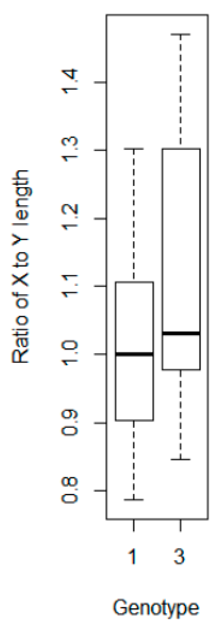
We compared the ratio of the leaf to stem weights for all three genotypes and found a similar ratio, suggesting variations in the stalk and stem weights may not be a factor in the variation in response between the single-scan subsampled methodology and the three genotypes (data not shown). However, when we compared the dimensions of the bounding boxes in CC for each of the plants in Genotypes 1 and 3, we found a significant difference (T = −1.77,
p-value 0.09) in the ratio of the X to Y axis lengths (
Figure 13). This suggests there is a statistical difference in the shape of the two genotypes, albeit one with only 90% confidence. Therefore, the bounding box method of determining the difference between single and multiple scans should be viewed with caution.
4. Discussion
The binned height biomass analysis did not work well (R2 0.01). Using the leaf weight did improve the correlation, though an R2 of 0.19 is not sufficient to suggest LiDAR as a phenotyping tool for binned height biomass determination. However, several factors could be the cause and might be addressed in the future. First, the bins may not have overlapped well in respect to the start and end positions in the LiDAR data versus the field data. Second, errors related to the placement of the bin start and end locations may have caused noise in the field data. One solution might be to mark the bins on the plant prior to scanning. This would allow more precise overlap to occur between the LiDAR and field data, which might improve the correlation. In addition, this would overcome some of the noise in the field data caused by the imprecise bin locations, further improving the result.
Depending on the processing workflow chosen for the LiDAR data, the strength of the correlation to the entire plant biomass changed. Two key differences existed between the processing workflows: (1) the use of a single scan per plant versus both scans registered together, and (2) if registered scans were used, whether or not the point cloud was further subsampled. It should be noted that all single-scan analyses included the further subsampling step. The use of the registered-only processing methodology resulted in marginal predictability of the entire plant biomass. However, when the same registered dataset was subsampled to produce a uniform point density, the correlation improved (R2 0.45 to 0.73). Skipping the time-consuming and labor-intensive step of registration, yet still applying the subsampling, resulted in the same R2 of 0.73. This result alone suggests there is no need to capture two scans of each cassava plant in order to correlate to the entire plant’s biomass, and the registration step can be skipped. This is a major finding, as much of the processing time is spent in the manual registration of scans.
The three genotypes used varied in their aboveground structure. Depending on the processing workflow used (registered and subsampled versus single-scan subsampled), we found the strength of the correlation to the entire plant weight changed, both between genotypes and within. For Genotypes 1 and 2, the use of the single-scan subsampled methodology is the best option. However, for Genotype 3, the use of the registered and subsampled method achieved superior results over the single-scan subsampled method.
The variation in the response of Genotype 3 between the two analysis methods mentioned previously sparked a comparison between the field-derived leaf weight and the LiDAR data. Initial speculation was that structural differences between the genotypes might cause variation in the amount of the stalk and stem weight. The stalks, and especially the stems, are hard to capture in the LiDAR data as these parts of the plant are often obscured from view by the leaves. By removing the weight of the stalks and stems, we thought we might improve the overall correlation, as well as improving the response of Genotype 3 to the single-scan subsampled analysis method. For Genotypes 1 and 3, using the leaf weight improved the correlation, as compared to regressing against the entire plant weight when the same processing methodology was considered (
Table 5 and
Table 6). For Genotype 2, the results were good irrespective of the method used, as can be seen in the minimal variation in the statistics between the entire plant and leaf analysis, as well as between the processing methods. However, using the leaf weight with the single-scan subsampled method resulted in an improved correlation for Genotype 1, but a lowered one for Genotype 3.
It is unclear why using the single-scan subsampled analysis workflow resulted in a similar, or even superior, correlation in all cases except that of Genotype 3. In seeking to understand this, we looked at the differences in the horizontal growth shape between Genotypes 1 and 3. We found that Genotype 1 had a more squared growth pattern with less variation between the plants, while Genotype 3 had a more rectangular growth pattern with more variation between plants. An example of this variation can be seen in
Figure 14, where an example plant from Genotype 1 has a nearly square bounding box, while the example plant from Genotype 3 has a more rectangular box. The combination of the more rectangular growth pattern with the greater variation in shape within Genotype 3 may be one cause of the poor performance of the single-scan subsampled analysis method for the genotype.
Genotype 3 may also provide the best example of what a campaign would look like in a field featuring a higher planting density. As this genotype contained low-hanging branches, it was more likely that there would be overlapping and indistinguishable points between the vegetation and the ground. However, there appeared to be no complications with the Progressive Morphological Filter’s classification of ground points, based on inspections by eye. However, while the filter proved effective for segmenting and eliminating ground points, eliminating points from overlapping leaves and branches would certainly prove more challenging. It is likely that any such overlap would have to be removed manually and thus would depend heavily on the skill of the user. While a TLS like the FARO Focus series provides a high-quality image, significant overlap in plants would make it very difficult to properly classify biomass based on point clouds. In this case, a cassava variety bred specifically for high-density planting (such as the asparagus type in this experiment) would be ideal for ground-based LiDAR phenotyping, as the erect structure would make overlap far less likely. It is also feasible that advances in machine learning could help to mitigate some of the challenges associated with differentiating between overlapping plants, especially if algorithms are designed specifically for this purpose. Scharr et al. have already had success using these methods with leaf segmentation in Arabidopsis and tobacco [
30], while Kartal et al. have had success segmenting overlapping bean plants using a k-means algorithm [
31]. For fields which feature dense planting, breeders may also receive better results by pursing large biomass assessments made through UAVs [
32].
5. Conclusions
This study was designed to determine several different ways of assessing cassava biomass in the field with an industry-standard TLS: binned height, full plant with registration and single scan. Results varied across these three methods, but ultimately the use of terrestrial laser scanners for biomass estimation of cassava appears to be suitable in most cases.
Binned height was the least successful method, providing poor correlations that would be unsuitable in every circumstance given the effectiveness of this technology in crop [
33,
34] and environmental [
35] biomass assessments. However, we believe that this was largely due to the experimental setup, which can be remedied for additional studies. In future work, binned field data will be collected using a marker system to allow the alignment of the field bins to those generated in the LiDAR data, assuring that more direct comparisons are made between the point clouds and dry material.
Estimating biomass using registered point clouds of the entire plant yielded far better results, especially when using a subsample of points from the clouds. However, this is also very much dependent upon the genotype and processing method. The erect shrub and low-branching genotypes improved when being compared to the leaf-only weight, while the asparagus type had only minor changes when being subjected to the same method. Likewise, the asparagus types had the best correlations across all processing methods. Thus, those breeders selecting for the asparagus genotype are likely to have the most reliable data.
Additionally, it is likely that the painstaking registration process previously assumed essential for these types of biomass estimations may not be necessary in the case of shrub crops, saving a substantial amount of time in the data collection and processing stages of LiDAR acquisition. Experiments using other crops and cassava genotypes, as well as those using other sensors where a point cloud is formed, will need to re-test the use of the single-scan subsampled processing workflow and provide a better assessment of the full potential of bypassing the registration step for biomass estimation and phenotyping in general. In addition, there is a significant need to determine what set of factors led to the poor performance of the single-scan subsampled processing methodology for Genotype 3.
In conclusion, our findings, while positive, suggest that there is not a single LiDAR processing workflow which can be applied to all cassava genotypes for the prediction of aboveground biomass. Therefore, additional preliminary testing is recommended before committing to a processing methodology.
Author Contributions
Conceptualization, T.A. and R.B.; methodology, T.A., R.B. and M.G.S.; software, H.R.; validation, T.A., R.B. and I.B.-P.; formal analysis, T.A., R.B. and I.B.-P.; investigation, R.B., H.R. and M.G.S.; resources, D.B.H. and M.G.S.; data curation, T.A., R.B. and I.B.-P.; writing—original draft preparation, R.B. and T.A.; writing—review and editing, R.B., T.A. and D.B.H.; visualization, R.B. and H.R.; supervision, D.B.H. and M.G.S.; project administration, D.B.H. and M.G.S.; funding acquisition, D.B.H. All authors have read and agreed to the published version of the manuscript.
Funding
This research was funded by The National Science Foundation, grant number 1543957 to Dirk B. Hays.
Institutional Review Board Statement
Not applicable.
Informed Consent Statement
Not applicable.
Data Availability Statement
Data available on request due to restrictions e.g., privacy or ethical. The data presented in this study are available on request from the corresponding author. The data are not publicly available due to sharing between academic and private institutions.
Acknowledgments
We wish to thank the reviewers for their time and insight provided in improving this paper, as well as the employees of the International Center for Tropical Agriculture (CIAT) in Palmira, Colombia, for the use of their facilities in completing this research.
Conflicts of Interest
The authors declare no conflict of interest. The funders had no role in the design of the study; in the collection, analyses, or interpretation of data; in the writing of the manuscript, or in the decision to publish the results.
References
- Fauquet, C.; Fargette, D. African cassava mosaic virus: Etiology, epidemiology and control. Plant Dis. 1990, 74, 404–411. [Google Scholar] [CrossRef]
- Nonchana, T.; Pianthong, K. Bio-oil Synthesis from Cassava Pulp via Hydrothermal Liquefaction: Effects of Catalysts and Operating Conditions. Int. J. Renew. Energy Dev. 2020, 9, 329–337. [Google Scholar] [CrossRef]
- Ojediran, T.K.; Durojaiye, V.; Adeola, R.G.; Ojediran, J.T. Awareness of Cassava Peel Utilization as a Feedstuff among Livestock Farmers in Ogbomoso Zone of Nigeria. Sci. Pap. Manag. Econ. Eng. Agric. Rural Dev. 2020, 20, 395–403. [Google Scholar]
- El-Sharkawy, M.A. Cassava biology and physiology. Plant Mol. Biol. 2003, 53, 621–641. [Google Scholar] [CrossRef]
- Montagnac, J.A.; Davis, C.R.; Tanumihardjo, S.A. Nutritional value of cassava for use as a staple food and recent advances for improvement. Compr. Rev. Food Sci. Food Saf. 2009, 8, 181–194. [Google Scholar] [CrossRef] [PubMed]
- Agbaeze, E.K.; Ohunyeye, F.O.; Obamen, J.; Ibe, G.I. Management of Food Crop for National Development: Problems and Challenges of Cassava Processing in Nigeria. SAGE Open 2020, 10, 1–13. [Google Scholar] [CrossRef]
- Nassar, N.M.A.; Ortiz, R. Cassava improvement: Challenges and impacts. J. Agric. Sci. 2007, 145, 163–171. [Google Scholar] [CrossRef] [Green Version]
- Busener, N.; Kengkanna, J.; Saengwilai, P.J.; Bucksch, A. Image-based root phenotyping links root architecture to micronutrient concentration in cassava. Plants People Planet 2020, 2, 678–687. [Google Scholar] [CrossRef]
- Olasanmi, B.; Akoroda, M.O.; Okogbenin, E.; Egesi, C.; Nwaogu, A.S.; Tokula, M.H.; Ukaa, G.T.; Agba, A.J.; Ogbuekiri, H.; Nwakor, W.; et al. Identification of cassava (Manihot esculenta Crantz) genotypes with early storage root bulking. J. Crop Improv. 2017, 31, 173–182. [Google Scholar]
- Latif, S.; Romuli, S.; Barati, Z.; Muller, J. CFD assisted investigation of mechanical juice extraction from cassava leaves and characterization of the products. Food Sci. Nutr. 2020, 8, 3089–3098. [Google Scholar] [CrossRef] [Green Version]
- Malik, F.; Suryani, S.; Ihsan, S.; Meilany, E.; Hamsidi, R. Formulation of Cream Body Scrub from Ethanol Extract of Cassava Leaves (Manihot esculenta) as Antioxidant. J. Vocat. Health Stud. 2020, 4, 21–28. [Google Scholar] [CrossRef]
- Okogbenin, E.; Fregene, M. Genetic analysis and QTL mapping of early root bulking in an F 1 population of non-inbred parents in cassava (Manihot esculenta Crantz). Theor. Appl. Genet. 2002, 106, 58–66. [Google Scholar] [CrossRef]
- Nweke, F.; Spencer, D.S.; Lynam, J.K. The Cassava Transformation: Africa’s Best Kept Secret; East Lansing, Michigan State University Press: Lansing, MI, USA, 2002; pp. 1–273. [Google Scholar]
- Nguyen, T.H.L.; Ngoan, L.D.; Bosch, G.; Verstegen, M.W.A.; Hendriks, W.H. Ileal and total tract apparent crude protein and amino acid digestibility of ensiled and dried cassava leaves and sweet potato vines in growing pigs. Anim. Feed Sci. Technol. 2012, 172, 171–179. [Google Scholar] [CrossRef]
- Alamu, E.O.; Nuwamanya, E.; Cornet, D.; Meghar, K.; Adesokan, M.; Tran, T.; Belalcazar, J.; Desfontaines, L.; Davrieux, F. Near-infrared spectroscopy applications for high-throughput phenotyping for cassava and yam: A review. Int. J. Food Sci. Technol. 2020, 56, 1491–1501. [Google Scholar] [CrossRef]
- Grotti, M.; Alivernini, A.; Calders, K.; Chianucci, F.; Ferrara, C.; Origo, N.; Puletti, N. An intensity, image-based method to estimate gap fraction, canopy openness and effective leaf area index from phase-shift terrestrial laser scanning. Agric. For. Meteorol. 2020, 280, 107766. [Google Scholar] [CrossRef]
- Jairo, S.M.; Bernardo, C.A.; Jhonys, P.B. Canopy architecture in cassava (Manihot esculenta Crantz) in tropical dry forest in Colombia. Colomb. J. Anim. Sci. 2017, 9, 271–280. [Google Scholar]
- Vosselman, G.; Maas, H.G. Airborne and Terrestrial Laser Scanning; Whittles Publishing: Dunbeath Mill, UK, 2010; pp. 1–318. [Google Scholar]
- Julin, A.; Kurkela, M.; Rantanen, T.; Virtanen, J.P.; Maksimainen, M.; Kukko, A.; Kaartinen, H.; Vaaja, M.T.; Hyyppä, J.; Hyyppä, H. Evaluating the Quality of TLS Point Cloud Colorization. Remote Sens. 2020, 12, 2748. [Google Scholar] [CrossRef]
- Hoffmeister, D.; Waldhoff, G.; Korres, W.; Curdt, C.; Bareth, G. Crop height variability detection in a single field by multi-temporal terrestrial laser scanning. Precis. Agric. 2016, 17, 296–312. [Google Scholar] [CrossRef]
- Höfle, B. Radiometric correction of terrestrial LiDAR point cloud data for individual maize plant detection. IEEE Geosci. Remote Sens. Lett. 2013, 11, 94–98. [Google Scholar] [CrossRef]
- Hosoi, F.; Omasa, K. Estimating vertical plant area density profile and growth parameters of a wheat canopy at different growth stages using three-dimensional portable LiDAR imaging. ISPRS J. Photogram Remote Sens. 2009, 64, 151–158. [Google Scholar] [CrossRef]
- Ehlert, D.; Horn, H.J.; Adamek, R. Measuring crop biomass density by laser triangulation. Comput. Electron. Agric. 2008, 61, 117–125. [Google Scholar] [CrossRef]
- Ehlert, D.; Adamek, R.; Horn, H.J. Laser rangefinder-based measuring of crop biomass under field conditions. Precis. Agric. 2009, 10, 395–408. [Google Scholar] [CrossRef]
- Ehlert, D.; Heisig, M.; Adamek, R. Suitability of a laser rangefinder to characterize winter wheat. Precis. Agric. 2010, 11, 650–663. [Google Scholar] [CrossRef]
- Keightley, K.E.; Bawden, G.W. 3D volumetric modeling of grapevine biomass using Tripod LiDAR. Comput. Electron. Agric. 2010, 74, 305–312. [Google Scholar] [CrossRef]
- Girardeau-Montaut, D. CloudCompare (Version 2.10 Beta) [Software]. 2017. Available online: https://www.danielgm.net/cc/ (accessed on 20 January 2018).
- Zhang, K.; Chen, S.C.; Whitman, D.; Shyu, M.L.; Yan, J.; Zhang, C. A progressive morphological filter for removing nonground measurements from airborne LiDAR data. IEEE Trans. Geosci. Remote Sens. 2003, 41, 872–882. [Google Scholar] [CrossRef] [Green Version]
- Efron, B.; Tibshirani, R.J. An Introduction to the Bootstrap; Chapman & Hall: New York, NY, USA, 1994; pp. 1–436. [Google Scholar]
- Scharr, H.; Minervini, M.; French, A.; Klukas, C.; Kramer, D.M.; Liu, X.; Luengo, I.; Pape, J.M.; Polder, G.; Vukadinovic, D.; et al. Leaf segmentation in plant phenotyping: A collation study. Mach. Vis. Appl. 2016, 27, 585–606. [Google Scholar] [CrossRef] [Green Version]
- Kartal, S.; Choudhary, S.; Stočes, M.; Šimek, P.; Vokoun, T.; Novák, V. Segmentation of Bean-Plants Using Clustering Algorithms. AGRIS OnLine Pap. Econ. Inf. 2020, 3, 36–43. [Google Scholar] [CrossRef]
- Cummings, A.R.; Karale, Y.; Cummings, G.R.; Hamer, E.; Moses, P.; Norman, Z.; Captain, V. UAV-derived data for mapping change on a swidden agriculture plot: Preliminary results from a pilot study. Int. J. Remote Sens. 2017, 38, 2066–2082. [Google Scholar] [CrossRef]
- Li, P.; Zhang, X.; Wang, W.; Zheng, H.; Yao, X.; Tian, Y.; Zhu, Y.; Cao, W.; Chen, Q.; Cheng, T. Estimating aboveground and organ biomass of plant canopies across the entire season of rice growth with terrestrial laser scanning. Int. J. Appl. Earth Observ. Geoinf. 2020, 91, 102132. [Google Scholar] [CrossRef]
- Fernández-Sarría, A.; López-Cortés, I.; Estornell, J.; Velázquez-Martí, B.; Salazar, D. Estimating residual biomass of olive tree crops using terrestrial laser scanning. Int. J. Appl. Earth Observ. Geoinf. 2019, 75, 163–170. [Google Scholar] [CrossRef]
- Guangpeng, F.; Liangliang, N.; Dong, Y.; Su, X.; Chen, F. AdQSM: A New Method for Estimating Above-Ground Biomass from TLS Point Clouds. Remote Sens. 2020, 12, 3089. [Google Scholar]
Figure 1.
Location of the International Center for Tropical Agriculture. Approximately 16 km east, northeast of Cali, Colombia. Location of the research center is represented by a star.
Figure 1.
Location of the International Center for Tropical Agriculture. Approximately 16 km east, northeast of Cali, Colombia. Location of the research center is represented by a star.
Figure 2.
Planting map, with 9 age groups, 3 genotypes (27 plots) and 15 plants per plot. Stars represent the planting location within a given plot.
Figure 2.
Planting map, with 9 age groups, 3 genotypes (27 plots) and 15 plants per plot. Stars represent the planting location within a given plot.
Figure 3.
Examples of the 3 cassava genotypes used in the study. (a) Erect shrub type (523-7), (b) asparagus type (Esparrago) and (c) low-branching type (HMC-1).
Figure 3.
Examples of the 3 cassava genotypes used in the study. (a) Erect shrub type (523-7), (b) asparagus type (Esparrago) and (c) low-branching type (HMC-1).
Figure 4.
LiDAR data processing and analysis protocol.
Figure 4.
LiDAR data processing and analysis protocol.
Figure 5.
Binned (20 cm) registered and subsampled point cloud data regressed against the leaf dry weight for all genotypes. (a) Regression, (b) bootstrap (n = 349).
Figure 5.
Binned (20 cm) registered and subsampled point cloud data regressed against the leaf dry weight for all genotypes. (a) Regression, (b) bootstrap (n = 349).
Figure 6.
Registered and subsampled point cloud data regressed against the entire plant dry weight for all genotypes. (a) Regression, (b) bootstrap (n = 54).
Figure 6.
Registered and subsampled point cloud data regressed against the entire plant dry weight for all genotypes. (a) Regression, (b) bootstrap (n = 54).
Figure 7.
Single-scan subsampled point cloud data regressed against the entire plant dry weight for all genotypes. (a) Regression, (b) bootstrap (n = 54).
Figure 7.
Single-scan subsampled point cloud data regressed against the entire plant dry weight for all genotypes. (a) Regression, (b) bootstrap (n = 54).
Figure 8.
Registered and subsampled point cloud data regressed against the entire plant dry weight, by genotype. (a) Regression, (b) bootstrap (n = 18).
Figure 8.
Registered and subsampled point cloud data regressed against the entire plant dry weight, by genotype. (a) Regression, (b) bootstrap (n = 18).
Figure 9.
Single-scan subsampled point cloud data regressed against the entire plant dry weight, Genotype 3. (a) Regression, (b) bootstrap (n = 18).
Figure 9.
Single-scan subsampled point cloud data regressed against the entire plant dry weight, Genotype 3. (a) Regression, (b) bootstrap (n = 18).
Figure 10.
Registered and subsampled point cloud data regressed against the leaf dry weight for all genotypes. (a) Regression, (b) bootstrap (n = 54).
Figure 10.
Registered and subsampled point cloud data regressed against the leaf dry weight for all genotypes. (a) Regression, (b) bootstrap (n = 54).
Figure 11.
Registered and subsampled point cloud data regressed against the leaf dry weight, Genotype 3. (a) Regression, (b) bootstrap (n = 18).
Figure 11.
Registered and subsampled point cloud data regressed against the leaf dry weight, Genotype 3. (a) Regression, (b) bootstrap (n = 18).
Figure 12.
Single-scan subsampled point cloud data regressed against the leaf dry weight, Genotype 3. (a) Regression, (b) bootstrap (n = 18).
Figure 12.
Single-scan subsampled point cloud data regressed against the leaf dry weight, Genotype 3. (a) Regression, (b) bootstrap (n = 18).
Figure 13.
Ratio of the X to Y dimension lengths by plant for Genotypes 1 and 3 (n = 18 per genotype).
Figure 13.
Ratio of the X to Y dimension lengths by plant for Genotypes 1 and 3 (n = 18 per genotype).
Figure 14.
Top-down view exported from CloudCompare showing the variation in the shape between Genotype 1 and Genotype 3. Bounding box in yellow.
Figure 14.
Top-down view exported from CloudCompare showing the variation in the shape between Genotype 1 and Genotype 3. Bounding box in yellow.
Table 1.
FARO Focus 120 scan settings.
Table 1.
FARO Focus 120 scan settings.
| Setting | Value |
|---|
| Resolution | 1/5 |
| Quality | 3X |
| Vertical Scan Area | −60° to 90° |
| Horizontal Scan Area | 0° to 180° |
| Scan Duration | 2 m 39 s |
| Point Distance | 7.67 nm at 10 m |
Table 2.
Statistical Outlier Removal (SOR) settings in CloudCompare.
Table 2.
Statistical Outlier Removal (SOR) settings in CloudCompare.
| SOR Function | Setting |
|---|
| Mean distance estimation | 6 points |
| SD multiplier threshold | 1.00 |
Table 3.
Progressive Morphological Filter (PMF) settings in R.
Table 3.
Progressive Morphological Filter (PMF) settings in R.
| PMF Function | Setting |
|---|
| Window Size | 0.2 m |
| Threshold Height | 0.05 m |
Table 4.
Registered and subsampled point cloud data regressed against the entire plant dry weight, by genotype. Bootstrap output (n = 18).
Table 4.
Registered and subsampled point cloud data regressed against the entire plant dry weight, by genotype. Bootstrap output (n = 18).
| Genotype | Mean R2 | Bias | STDEV | 95% Confidence Interval |
|---|
| 1 | 0.66 | 4.84 × 10⁻³ | 0.10 | 0.36–0.81 |
| 2 | 0.96 | 1.37 × 10⁻³ | 0.01 | 0.92–0.98 |
| 3 | 0.73 | −7.65 × 10⁻³ | 0.12 | 0.40–0.88 |
Table 5.
Regression and bootstrap results by analysis method using both the dry plant weight and leaf weight for all genotypes (n = 54) and by genotype (n = 18). R = registered; R & S = registered and subsampled; SS & S = single-scan subsampled. Gray color denotes R2 below 0.7.
Table 5.
Regression and bootstrap results by analysis method using both the dry plant weight and leaf weight for all genotypes (n = 54) and by genotype (n = 18). R = registered; R & S = registered and subsampled; SS & S = single-scan subsampled. Gray color denotes R2 below 0.7.
| Comparing | All Genotypes
Regression Bootstrap |
|---|
| Analysis Method | Plant Weight | Leaf Weight | R2 | p-Value | 95% CI |
|---|
| R | X | | 0.45 | 1.73 × 10⁻⁸ | 0.21–0.70 |
| R & S | X | | 0.73 | 1.26 × 10⁻¹⁶ | 0.55–0.84 |
| SS & S | X | | 0.73 | 2.20 × 10⁻¹⁶ | 0.57–0.84 |
| R & S | | X | 0.80 | 2.00 × 10⁻¹⁶ | 0.63–0.88 |
| SS & S | | X | 0.78 | 2.00 × 10⁻¹⁶ | 0.64–0.86 |
Table 6.
Regression and bootstrap results by analysis method using both the dry plant weight and leaf weight for by genotype (n = 18). R = registered; R & S = registered and subsampled; SS & S = single-scan subsampled. Gray color denotes R2 below 0.7.
Table 6.
Regression and bootstrap results by analysis method using both the dry plant weight and leaf weight for by genotype (n = 18). R = registered; R & S = registered and subsampled; SS & S = single-scan subsampled. Gray color denotes R2 below 0.7.
| Comparing | Genotype 1
Regression Bootstrap | Genotype 2
Regression Bootstrap | Genotype 3
Regression Bootstrap |
|---|
| Analysis Method | Plant Weight | Leaf Weight | R2 | p-Value | 95% CI | R2 | p-Value | 95% CI | R2 | p-Value | 95% CI |
|---|
| R & S | X | | 0.64 | 4.32 × 10⁻⁵ | 0.36–0.81 | 0.95 | 1.12 × 10⁻¹² | 0.92–0.98 | 0.71 | 6.45 × 10⁻⁶ | 0.40–0.88 |
| SS & S | X | | 0.73 | 3.55 × 10⁻⁶ | 0.45–0.88 | 0.96 | 9.29 × 10⁻¹³ | 0.92–0.98 | 0.52 | 4.38 × 10⁻⁴ | 0.15–0.79 |
| R & S | | X | 0.70 | 8.66 × 10⁻⁶ | 0.33–0.88 | 0.95 | 3.35 × 10⁻¹² | 0.91–0.98 | 0.83 | 1.13 × 10⁻⁷ | 0.58–0.94 |
| SS & S | | X | 0.76 | 1.64 × 10⁻⁶ | 0.45–0.91 | 0.94 | 3.82 × 10⁻¹¹ | 0.89–0.97 | 0.64 | 4.31 × 10⁻⁵ | 0.30–0.86 |
| Publisher’s Note: MDPI stays neutral with regard to jurisdictional claims in published maps and institutional affiliations. |
© 2021 by the authors. Licensee MDPI, Basel, Switzerland. This article is an open access article distributed under the terms and conditions of the Creative Commons Attribution (CC BY) license (http://creativecommons.org/licenses/by/4.0/).


 and
and 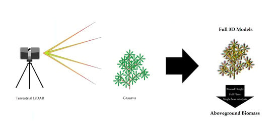


