Article

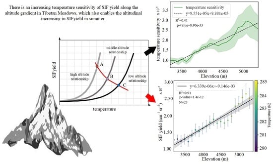
Satellite-Based Observations Reveal the Altitude-Dependent Patterns of SIFyield and Its Sensitivity to Ambient Temperature in Tibetan Meadows

1
Key Laboratory of Digital Earth Science, Aerospace Information Research Institute, Chinese Academy of Sciences, Beijing 100094, China
2
College of Resources and Environment, University of Chinese Academy of Sciences, Beijing 100049, China
*
Author to whom correspondence should be addressed.
Submission received: 16 February 2021 / Revised: 25 March 2021 / Accepted: 1 April 2021 / Published: 5 April 2021
(This article belongs to the Special Issue Remote Sensing of Fluorescence, Photosynthesis and Vegetation Status)

Abstract

:
Photosynthesis and its sensitivity to the changing environment in alpine regions are of great significance to the understanding of vegetation–environment interactions and other global ecological processes in the context of global change, while their variations along the elevation gradient remain unclear. Using solar-induced chlorophyll fluorescence (SIF) derived from satellite observations, we discovered an increase in solar-induced fluorescence yield ( S I F y i e l d ) with rising elevation in Tibetan meadows in the summer, related to the altitudinal variation in temperature sensitivity at both seasonal and interannual scales. Results of the altitudinal patterns of S I F y i e l d demonstrated higher temperature sensitivity at high altitudes, and the sensitivity at the interannual scale even exceeds that at seasonal scale when the elevation reaches above 4700 m. This high-temperature sensitivity of S I F y i e l d at high altitudes implies potential adaptation of alpine plants and also indicates that changes in photosynthesis-related physiological functions at high altitudes should receive more attention in climate change research. The altitudinal S I F y i e l d patterns revealed in this study also highlight that variations in temperature sensitivity should be considered in models, otherwise the increasing trend of S I F y i e l d observations can never be discovered in empirical simulations.

Graphical Abstract

1. Introduction

The photosynthesis activity of alpine vegetation and its response to the changing environment has been an attractive topic for centuries [1,2] due to its unparalleled scientific and social significance. In alpine regions, plants along the altitudinal gradient usually habituate themselves well to local environmental conditions, thus their physiological traits vary over relatively short horizontal distances [1,3]. Due to the unique combination of extreme environmental stresses along the altitude gradient, such as low temperature and high light intensity, large amounts of special materials for evolutionary studies on adaptation strategies can be found in alpine regions, which appeals to numerous ecologists and evolutionists [1,3,4,5,6]. The special combination of environmental stresses also makes the alpine area a natural laboratory for vegetation–climate interaction research. Environmental variables that often appear with collinearity decouple along the elevation gradient, which can be of benefit in clarifying the response of photosynthesis to the environment under wild conditions [1]. Considering the specificity of this habitat, the findings and mechanisms of adaptation in high-altitude regions can be different from those in other regions, such as high-latitude regions [7], therefore, research on the alpine vegetation–climate interaction is invaluable. Understanding the altitudinal variations in unique traits of alpine plants and their environmental sensitivity will help in revealing their adaptation mechanism in mountain areas, describing the impact of climate change on vegetation, and predicting the degree of biological negative feedback to the changing climate. However, the altitudinal patterns of vegetation changes are still under discussion.
Altitudinal factors can affect vegetation in diverse aspects. Studies have demonstrated that the phenological behavior of vegetation in alpine regions varies significantly with altitude. Liu et al. discovered higher phenological sensitivity to temperature in spring in regions with higher altitudes, which highlights the vulnerability of alpine vegetation in the context of global warming [8]. This study also found a reduced number of accumulated growing degree days before the growing season at high altitudes, which was consistent with the growth efficiency hypothesis suggesting that less heat is required for the green-up date in colder habitats. Apart from phenological properties, studies have also demonstrated that vegetation structure and some physiological traits change along with altitude [9,10]. Alpine plants were found to adjust their individual plant biomass allocation in the Tibetan Plateau [11,12]. According to that research, as altitude increases, plants increase their biomass proportion to below-ground storage organs in order to resist environmental stress. Ground research on variations in 13 traits of grassland and forest in the European Alps also demonstrated variations of plants along the elevation gradient, showing that stress factors such as cold and a short growing season can impact the growth and reproduction of alpine plants and constrain them to a limited number of strategies [13]. Based on published data on 210 species at 25 sites, a re-analysis study successfully modeled increasing photosynthetic capacity and decreasing primary production along the Amazon–Andes, and managed to test the emerging theory that photosynthetic traits and primary production depend on optimal acclimation and adaptation to the environment [14]. These results suggest that plants’ adaptation to their unique local circumstances can play an important role in the formation of altitudinal trait differences. Variations in phenotypes across altitudes generally reflects the long-term effects of harsh environmental conditions and short growing seasons on vegetation in higher regions [15].
However, it is still unclear whether and how these altitudinal factors influence photosynthesis-related traits and the sensitivity of these traits to environmental changes, and different results may be obtained in different regions [2]. While previous studies based on field investigations discovered altitudinal variations in the photoprotection strategies, photosynthetic parameters, and biochemical composition of the photosynthetic apparatus [13,16,17], the insufficient representativeness of field investigation limits the applicable range of these conclusions. Models do contribute to explaining photosynthetic changes along the altitude [2,14], but their oversimplified process and the complexity of the real world make it hard for them to show the diverse altitudinal patterns in the real world. Therefore, further studies are required to give an overall view of photosynthesis and its sensitivity to environmental changes at the ecosystem scale. Gross primary production (GPP) estimation products provide an opportunity to study photosynthesis productivity directly, but they are still insufficient to capture the spatial distribution of photosynthesis in some places. For instance, the data-driven FLUXCOM GPP products, derived from observations of the global micrometeorological flux site network (FLUXNET), is considered to be biased when applied to alpine regions, because the network’s EC towers are generally located in the temperate zone of the northern hemisphere below 1000 m [18].
As a special photosynthesis-related physiological trait detectable from remote distances, solar-induced chlorophyll fluorescence (SIF) has paved the way for research on altitudinal variations in the physiological status of alpine vegetation at large scale. Linked with light reaction in the photosynthetic process, SIF is emitted by light-inspired chlorophyll molecules and contains photosynthesis-related physiological information in addition to absorbed light information. Thus, it is able to reflect photosynthetic-related physiological responses of alpine vegetation to the environment. Numerous satellite-based SIF products have been developed [19,20,21,22,23,24] since the first satellite-based SIF retrieval in 2007 [25], which is valuable in places that lack ground observations, such as alpine regions. SIF contains information on both incident light intensity and plant properties, whereas SIFyield, derived from SIF normalized by absorbed photosynthetically active radiation (APAR), can be used to reflect photosynthetic traits of plants [26] as well as their responses to environmental stress [27,28]
Previous studies have observed the effect of altitude on photosynthesis in various regions by various methods, and their results involved different latent factors and revealed different mechanisms [1]. Here, based on the Global Ozone Monitoring Experiment 2 (GOME-2) satellite-based SIF dataset on the Tibetan Plateau meadow, we aim to (1) investigate and compare the relationship between altitude and SIFyield from different perspectives, which may involve the influence of vegetation adaptation, seasonal changing factors, and interannual environmental changes; (2) find whether there is variation in the temperature sensitivity of SIFyield along the altitude gradient; and (3) find the spatial distribution of temperature sensitivity in the study area and compare the temperature sensitivity of SIFyield to seasonal changes and to interannual changes, which may help us find areas that need extra attention in the context of global change.

2. Materials and Methods
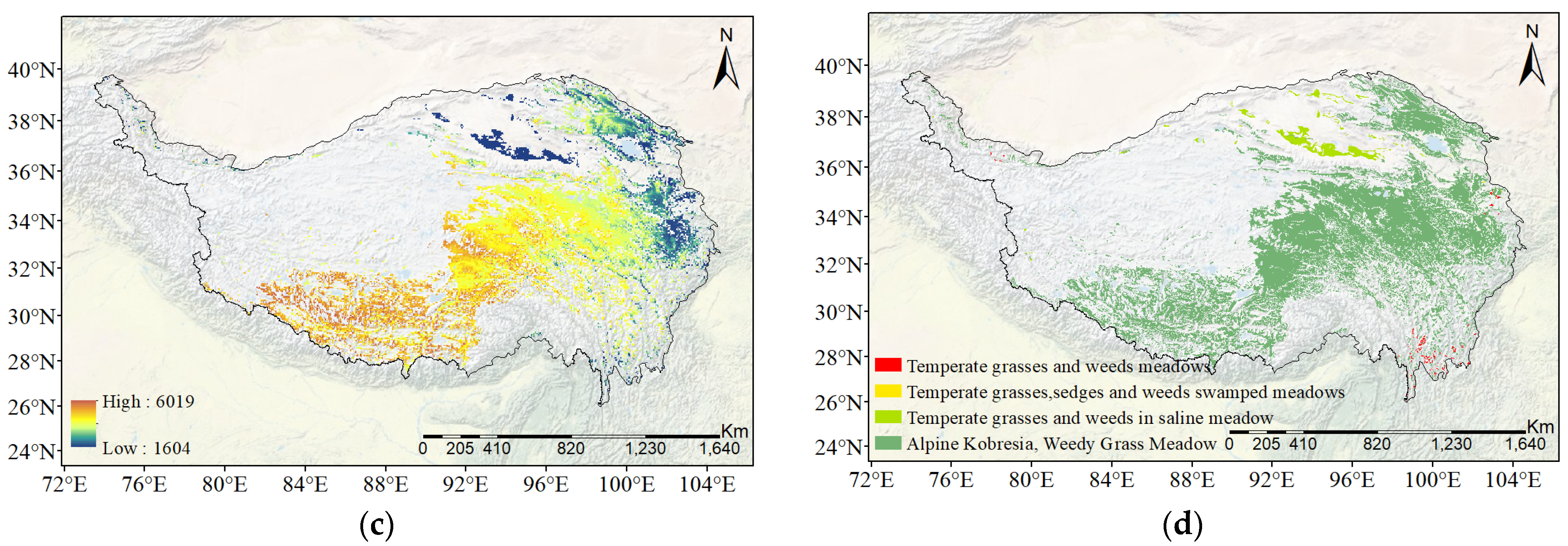
2.1. Study Region

The Tibetan Plateau is a particularly special alpine area and has aroused much interest. As a result of the unique unstable environmental conditions caused by the thin atmosphere and the extreme stress combination of low air pressure, strong winds, high ultraviolet light, high rates of warming, and large daily temperature amplitude, plants in such high-altitude regions face even tougher living conditions than those in boreal areas [29,30,31]. For example, alpine plants have to cope with stress imposed by low temperature and high light intensity, otherwise they would suffer from oxidative damage triggered by an imbalance between energy absorption and energy use [32,33,34,35]. In a subtropical high-altitude region, this imbalance problem is reinforced, therefore, the vegetation may exhibit more interesting traits, as well as unusual photosynthesis behaviors [31].
The Tibetan Plateau has attracted much attention, not only because of its extremely high altitude and unique environment, but also for its high sensitivity to climate change [30,36,37] and its great significance to human lives. Recognized as one of the most sensitive areas to climate warming, this region has aroused much attention, and studies have shown an accelerated, higher rate of warming in the Tibetan Plateau than the global average [38,39]. As the “third pole” of the earth, the Tibetan Plateau influences the atmospheric circulation and participates in the formation and modulation of the Asian monsoon climate [40,41,42,43]. In addition, it can also regulate the quantity and quality of water in many important rivers in the world [44], which shows the essential role it plays in human life. The ecosystem of the plateau plays an important environmental role throughout Asia [45]. If the ecosystem collapses due to drastic environmental change, it may even cause air pollution in the lowland area, because it has all the factors and conditions to generate dust storms in the Tibetan Plateau [46]. Since photosynthesis makes a significant contribution to ecosystem development, the study of alpine photosynthesis traits and response to changing environmental conditions may help us foresee the fate of alpine ecosystems.

2.2. Satellite-Based SIF Dataset

SIF retrievals during 2007–2018 were utilized in this study. The SIF data came from an 8-day spatially downscaled gridded GOME-2 SIF dataset with resolution of 0.05° [47]. It is based on robust and cloud-insensitive GOME-2 SIF retrieval at 740 nm wavelength proposed by Köhler et al. (2015) and shows high agreement with the observations of TROPOMI after bias correction. As the original retrieved SIF represents the instantaneous value at its observation time, daily correction was performed to convert the instantaneous SIF to the daily average SIF. The SIF values in Duveiller’s dataset were converted to daily average via the method proposed by Köhler et al. [23], and are therefore comparable with daily gross primary production (GPP). In addition, rigorous quality control was performed on this dataset, and the impacts of bidirectional reflectance and weather conditions were minimized. However, it should be noted that since day correction was performed using the cosine of the solar zenith angle (SZA), variations in weather during the day are not taken into account in this dataset. Therefore, the so-called daily correction is actually a correction for the difference in solar zenith angle and day length caused by latitudes, and all of the SIF data used in this research can be seen as clear sky observations. In this study, instantaneous SIF at 09:30 was obtained by conducting the inverse operation of previous steps for the calculation of instantaneous S I F y i e l d .
Although GOME-2 provides global satellite-based SIF data covering a long period of time, the radiometric degradation of the instrument is problematic and may lead to inconsistency in interannual analysis [48,49]. In order to address that, a pseudo-invariant method was employed to correct for this degradation in a dataset shared in ZENODO repository [50].

2.3. Datasets of Environment Variables

The variables used to represent ambient thermal conditions in this study were acquired from the China Meteorological Forcing Dataset (1979–2018) [51,52] and ERA5-Land hourly data from 1981 to the present [53]. The China Meteorological Forcing Dataset (CMFD) was developed specifically for studies in China and combines remote sensing products, reanalysis datasets, and in situ observations with a temporal resolution of 3 h [51]. Here we selected the daily 2 m air temperature CMFD product from 2007–2018 with a spatial resolution of 0.1° as the temperature variable.
We also applied the temperature variables from the ERA5-Land dataset to examine the robustness of the results in this research [52]. ERA5-Land is a reanalysis dataset with inputs used to control the uncertainty of simulations, and its hourly data provide estimations of numerous environmental variables with a spatial resolution of 0.1°. The 2 m temperature (unit: K) and skin temperature (unit: K) were selected to describe the overall thermal condition in the study area.
Photosynthetically active radiation (PAR) was obtained from the surface solar radiation downward product in the ERA5-Land hourly dataset by multiplying by a coefficient of 0.46. As the raw data provided by ERA5-Land represent accumulated values and the unit is J m−2, a conversion process was conducted and the unit was converted to W m−2. PAR at 09:30 (approximately the overpass time of GOME-2) was calculated in this research. Since the reanalyzed dataset gives the data at a certain universal time, data values in different pixels actually represent PAR values at different local times, which is different from satellite data. Therefore, time zone conversion was required here. The study area spans three time zones, so it was necessary to calculate the difference of accumulated PAR between the local 09:00 and 10:00 to obtain values at 09:00–10:00 for each time zone. The result can be approximately considered as instantaneous PAR at 09:30. Since directly mosaicked images have more obvious seams, corrections based on the sun zenith angle were performed within the time zone according to the central meridian and latitude differences.

2.4. DEM Data

For elevation data, we employed processed Shuttle Radar Topography Mission (STRM) data version 4.1 downloaded from International Center for Tropical Agriculture Consortium for Spatial Information SRTM (CIAT-CSI SRTM) [53]. The original dataset was derived from the United States Geological Survey (USGS)/NASA SRTM, and its no-data regions have been filled using interpolation methods described by Reuter et al. [54]. CIAT provides seamless, continuous topography surfaces at 250 m spatial resolution, and we resampled it to 0.05° to match the spatial resolution of SIF datasets. Considering the natural distribution of meadows in the Tibetan Plateau and possible misclassified regions in the vegetation map, regions above 5500 m and below 3200 m were discarded in the subsequent analysis. DEM values were binned at 100 m intervals.

2.5. Other Auxiliary Datasets

Besides the most important SIF data, environmental variables, and elevation data, some other datasets were also used as auxiliaries. The shapefile of the study region was acquired from the Datasets of the Boundary and Area of the Tibetan Plateau by Zhang [55,56]. It was employed as a mask layer and applied to every raster file in this study. According to this shapefile, the study area ranges from 25°59′37″N to 39°49′33″N, 73°29′56″E to 104°40′20″E, and spans three time zones, which indicates a need for time zone correction during the instantaneous PAR calculation process mentioned in Section 2.3.
The absorbed photosynthetically active radiation (APAR) represents the amount of photosynthetically active radiation absorbed by plants. In order to eliminate the impact of this total energy on SIF, APAR is required in this study. APAR can be calculated by multiplying the fraction of absorbed photosynthetic active radiation (fPAR) and PAR. Here in this study, we employed GLASS fraction of absorbed photosynthetic active radiation (fPAR) data [56,57]. The files in this dataset are organized in Geotiff format with 0.05° resolution, and the APAR data can be easily obtained by multiplying fPAR and spatially downscaled 0.05° PAR. Instantaneous APAR at 09:30 (approximately the overpass time of GOME-2) are generated in this research.
To extract the meadow region in the study area, we employed a vegetation map provided by the Institute of Botany, Chinese Academy of Sciences [58]. This thematic map is based on field investigations and shows the distribution and geographical patterns of vegetation in China, including horizontal and vertical distribution, in detail.

2.6. Statistical Analysis

According to previous studies, SIF can be expressed as the product of APAR and S I F y i e l d [26,59]. Therefore, S I F y i e l d is represented by the following formulation:
S I F y i e l d =   S I F A P A R =   S I F P A R × f P A R
S I F y i e l d can be treated as normalized SIF, getting rid of the impact of incident light intensity. Thus, it can indicate the SIF emission capacity of plants. Instantaneous S I F y i e l d (at about 09:30) was analyzed in this study to discuss the uncertainty caused by varying light conditions. Calculating instantaneous S I F y i e l d requires converting daily SIF data, provided by Duveiller, to instantaneous SIF at about 09:30. The conversion method is based on the cosine of SZA and is similar to the instantaneous PAR conversion inside the time zone, as mentioned above.
In our analysis, S I F y i e l d observations from 2007–2018 were aggregated to a temporal interval of 8 days or 1 month, in order to support the investigation of S I F y i e l d changes along the elevation gradient. According to the time resolution of the SIF observations, a total of 46 altitudinal S I F y i e l d variations for 8-day SIF and 12 for monthly SIF were obtained. Altitudinal variations in S I F y i e l d were observed first, then the seasonal and interannual changes of the variation patterns were analyzed. Seasonal changes of S I F y i e l d were investigated based on the multi-year average, and the relationship between S I F y i e l d and ambient temperature was explored. Considering the possible altitude-specific patterns, we also employed the observations at different altitudes to find out whether there were differences in the S I F y i e l d –temperature relationships. For analysis at the interannual scale, relationships between SIFyield and ambient temperature or PAR were investigated at different days of the year (DOYs), and the results obtained during the peak growth period are discussed.
We also analyzed the altitudinal variations in S I F y i e l d temperature sensitivity at seasonal and interannual scales. Sensitivity of S I F y i e l d to ambient temperature changes is defined as the slope of the linear model between S I F y i e l d and temperature in this study (the relationship can be expressed as a linear function only when the temperature reaches 275 K, a relatively mild temperature condition for alpine vegetation), thus it is also the indicator of the relationship between S I F y i e l d and temperature. Linear regressions on the relationship between S I F y i e l d and temperature were employed for the calculation of temperature sensitivity at both seasonal and interannual scales; in addition, the relationship between the altitudes and temperature sensitivity (the slopes of these linear regressions above) is also investigated by regression analysis. To identify areas sensitive to climate change, we took the seasonal temperature sensitivity at each altitude as the reference and then compared the interannual results with it. In order to visualize the spatial distribution of temperature sensitivity, linear regression analysis was conducted pixel by pixel, and the statistical significance of regression was also investigated here.
As a nonparametric test without requiring normal distribution [60], the Mann–Kendall trend test was employed to judge the monotonic trend of S I F y i e l d and temperature sensitivity series and indicate whether they were significant by inspecting the value of tau statistics. In addition, the Mann–Kendall test can also tell us whether there is an abrupt change in data series [61]. By observing the intersection point of the UF and UB statistics, we can locate the abruption. If there is only one intersection point and it falls into the confidence interval (usually defined as between +1.96 and −1.96), it indicates that there is an abrupt change in the series and it is significant at the given level. In this study, this method was employed to find the turning temperature threshold in seasonal S I F y i e l d changes along the elevation gradient. Additionally, the Wilcoxon rank sum test, another nonparametric test, was employed to determine whether there was a significant difference in temperature sensitivity of S I F y i e l d between low and high altitude.

3. Results

3.1. Altitudinal Patterns of SIFyield Changes

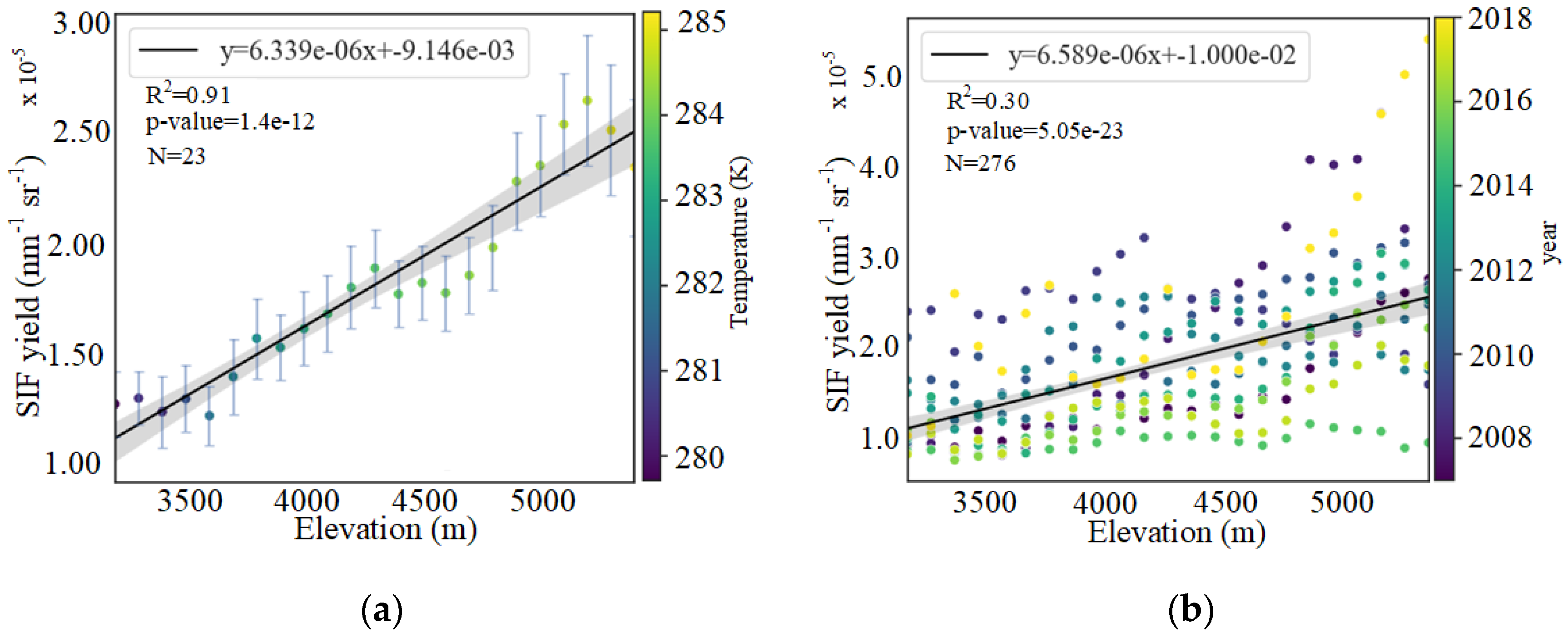
3.1.1. Altitudinal Variation in SIFyield

The S I F y i e l d changes along the elevation gradient shows an increase in values at higher elevation on summer days in the Tibetan Plateau. From DOY 173 (21 or 22 June) to DOY 245 (1 or 2 September), 8 out of 10 records (with 8-day intervals) support the increase in S I F y i e l d at high altitudes in summer, and the increase trend is particularly apparent on DOYs 197, 205, 213, and 221. On DOY 197 (14 or 15 July, in summer), S I F y i e l d increases along the altitude gradient, while the ambient temperature decreases simultaneously, as shown in Figure 1a. The coefficient of determination of the linear regression between S I F y i e l d and altitude is fairly high (R2 = 0.91) on DOY 197 for the 12-year averaged observations (Figure 1a). This high R2 value demonstrates that the elevation itself can explain nearly 91% of variations in S I F y i e l d in general, while the much weaker correlation (Figure 1b) shows that the discrepancy of S I F y i e l d in different years still exists, probably due to the impacts of other factors. The increased S I F y i e l d (Figure 1a) passed the Mann–Kendall trend test with p < 0.05, which confirms the significance of the trend. The trends of S I F y i e l d generally increase in high-altitude regions each year, as shown in Figure 1b. Both results displayed in Figure 1a,b confirm an increasing trend of S I F y i e l d along the elevation gradient, but the coefficient of determination of the linear regression in Figure 1b is much lower than that in Figure 1a. This might be explained by the stochastic field theory. If the distribution of SIF yield is considered as a stochastic field, the values of SIF yield taken at different elevations will be stochastic variables taken with a certain probability, thus the averaging process can bring down the uncertainties as listed in Figure 1a. Although S I F y i e l d varies in different years, there are apparent increasing trends of S I F y i e l d along the elevation gradient for most of the years (9 out of 12 in Figure 1b). This phenomenon suggests that the average pattern of higher S I F y i e l d along the altitude in summer (Figure 1a) is not the result of high-value anomalies in particular years (such as relatively high S I F y i e l d at high altitudes in 2018, Figure 1b).
Figure 2 shows observations from 12 years and compares the altitudinal S I F y i e l d changes in each year on DOY 197 and 149, and the results confirm that there are indeed occasions when S I F y i e l d increases as the elevation goes up, but it is not always correct. In Figure 2a, 10 out of 12 years (except 2009, 2012) follow the rule demonstrated in Figure 1a (DOY 197, in summer), while only 2 year (2010, 2015) in Figure 2b (DOY 149) obey the rule. Despite large interannual variations in S I F y i e l d (and there also seems to be atypical values associated with 2018 compared to other years), an increasing trend of S I F y i e l d along the altitude gradient can still be found for each year in summer (Figure 2a). Therefore, it seems that the interannual variation in S I F y i e l d mainly causes the systematic differences in absolute S I F y i e l d values among years, but it does not change the relative relationship among S I F y i e l d at different altitudes in each year. Interestingly, although the S I F y i e l d is usually larger at higher elevation in summer, there are still exceptional cases (for example, 2009 in Figure 2a, when S I F y i e l d at high altitudes is lower than in low altitudes). This phenomenon may be caused by phenological changes in different years, but other possibilities cannot be excluded based on the limited knowledge in this research.
Figure 3 illustrates seasonal changes of SIF and S I F y i e l d , as well as potentially related ambient environment variables (PAR and air temperature). As shown in Figure 3a, altitudinal variation in SIF seasonal changes is especially apparent. However, getting rid of the influence of APAR (which contains the impact of structure and incident light), S I F y i e l d still exhibits altitudinal differences, particularly in summer (although not as significant as SIF). This result may indicate the existence of altitudinal variation in physiological properties. SIF is lower at higher altitudes according to Figure 3a, whereas the altitudinal trend of S I F y i e l d is the inverse in the middle of the growing season (from approximately DOY 181 to 245), as shown in Figure 3b.
Different positions of peaks among these four variables are also found in Figure 3. The peak time of PAR is the earliest, and the others are far behind. Whereas the SIF peak time is slightly earlier and closer to the PAR peak, the peaks of S I F y i e l d and temperature are extremely close and become the latest ones. The synchronicity of S I F y i e l d and temperature dynamics indicates that S I F y i e l d may be relevant to ambient temperature on the seasonal scale. However, from about DOY 120–200, PAR starts to decrease, but the value of S I F y i e l d continues to increase at this time, indicating that the change of S I F y i e l d cannot be explained well by PAR. In contrast, due to the temperature lapse along the altitude gradient, the thermal condition in alpine regions is not ideal, thus when it gets warmer, physiological activities (reflected by S I F y i e l d ) are prone to increase sharply.
The SIF and S I F y i e l d peaks are both delayed at high elevations (Figure 3), but the altitudinal effects on their seasonal changes are not always the same. For SIF, it starts to increase earlier and grow faster at lower altitudes in spring; however, for S I F y i e l d , the growth rate shows no significant differences at different altitudes. In addition, SIF in low altitude regions also declines later than in higher places, as shown in Figure 3a, but S I F y i e l d declines earlier in low land regions.
As temperature can influence SIF and S I F y i e l d significantly, their responses to the temperature along the altitude gradient were also investigated (Figure 4). Contrary to the result in Figure 3b showing similar S I F y i e l d increasing rates with DOY at different altitudes in spring, the increasing rates of S I F y i e l d with temperature vary along the altitude (Figure 4b). Although both SIF and S I F y i e l d in Figure 4 show a positive correlation with temperature in the range of 260–280 K, the altitudinal differences in temperature response of S I F y i e l d are much larger than those of SIF. This indicates that the response of S I F y i e l d to temperature at the seasonal scale should not be expressed as a single linear function, but a set of functions that account for the differences in altitude. For SIF, however, the S I F y i e l d variations may be covered by APAR variations along the altitudinal gradient, and a linear regression can be applied to generalize the response of SIF at different altitudes, as shown in Figure 4a.
Despite the lower SIF at higher altitudes (Figure 4a), the vegetation there appears to have relatively high S I F y i e l d for a given temperature. For S I F y i e l d changes at the seasonal scale, there is also altitudinal variation in the slopes of the S I F y i e l d –temperature relationship (Figure 4b). As the temperature goes higher, S I F y i e l d increases faster, especially in high-altitude regions. However, when the temperature reaches about 275 K, the increase rate becomes stable and the relationship between S I F y i e l d and temperature can finally be described by linear regression. In general, the increasing trend of S I F y i e l d is reinforced significantly when the temperature is higher than 275 K.

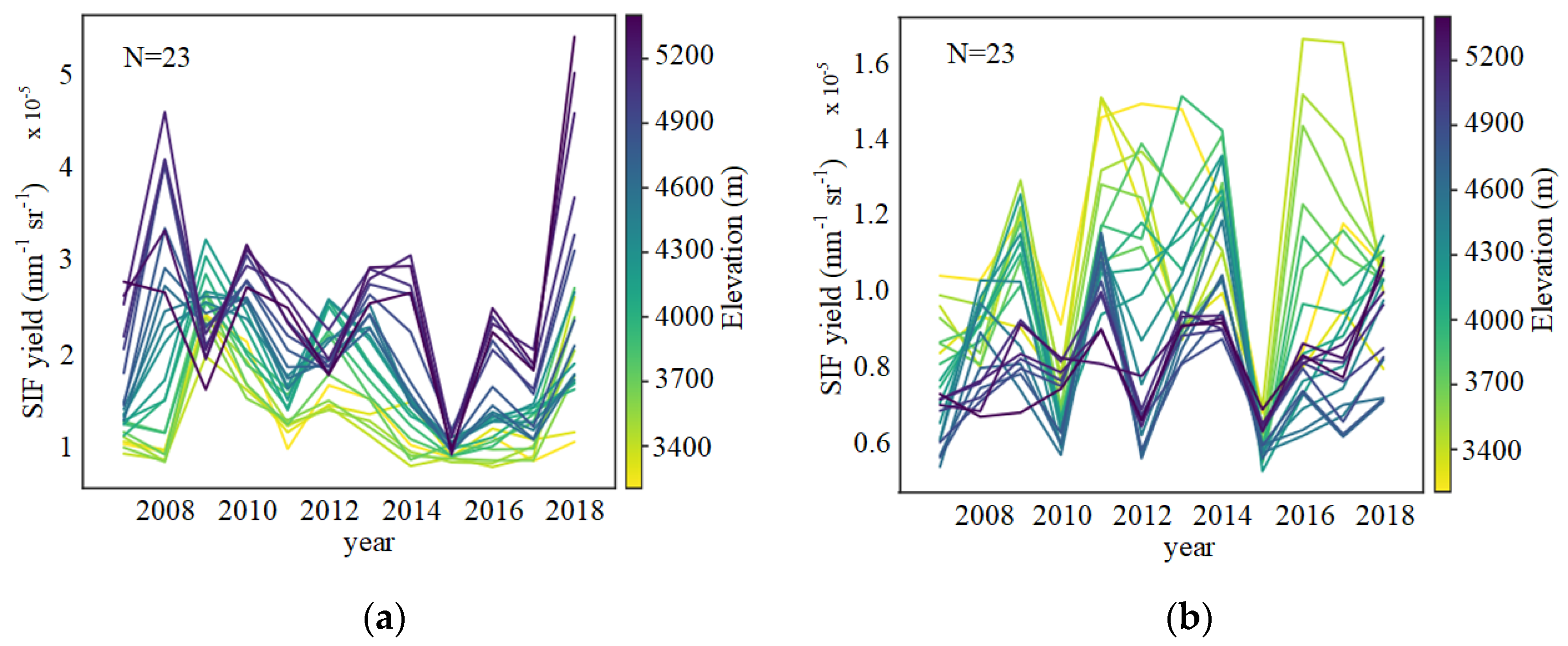
3.1.2. Altitude-Dependent SIFyield Changes at Interannual Scale

Since the growing stage of plants, the latitude of the subsolar point, and other climatic conditions at a specific site are usually similar on the same DOY in different years, the analysis of S I F y i e l d variation at interannual scale is less disturbed by these latent variables. Whereas seasonal changes in environmental conditions, differences in the vegetation growth stage, and altitudinal variations in the species composition of the ecosystem usually confound the altitudinal variation results derived from other perspectives, they are no longer the dominant factors for altitudinal S I F y i e l d variation at the interannual scale. Therefore, the variation pattern investigated from this aspect can be quite different from the patterns described above.
Figure 5a shows the changing relationships between S I F y i e l d and environment variables (PAR and air temperature) from DOY 133–277. As the figure depicts, the R2 of the S I F y i e l d –PAR relationship is high and stable throughout the period, while the R2 of the S I F y i e l d –temperature relationship is small and changeable, especially during the middle of the growing season. Since R2 shows the ability of independent variables to explain the variation in S I F y i e l d , the smaller R2 of temperature in summer indicates that the thermal condition can no longer explain the S I F y i e l d variation well, probably because it is good enough at that time. However, for PAR, R2 stays relatively high. It explains the S I F y i e l d well, which is not surprising, as excessive light is a common stress in alpine regions. In addition to the changing R2, the direction of the S I F y i e l d –temperature correlation is also unstable (Figure 5a), whereas the correlation between S I F y i e l d and PAR remains negative during the study period.
Based on the 12-year observations, Figure 5b shows the relationship between S I F y i e l d and PAR at different altitudes on DOY 205. As shown in Figure 5b, the responses of S I F y i e l d to the same environmental variable, PAR, are different in different habitats. Generally, it seems that S I F y i e l d at high altitude is still higher and is more sensitive to changes in PAR. Results obtained this way may be comparable to some experimental results obtained in the laboratory, as they are concentrated on the temporal changes of the same vegetation, and the change of vegetation itself is almost negligible. Nevertheless, differences may still exist, as the former results are more “authentic”. Because the observations come from complicated natural conditions, these results are difficult to simulate in the laboratory.

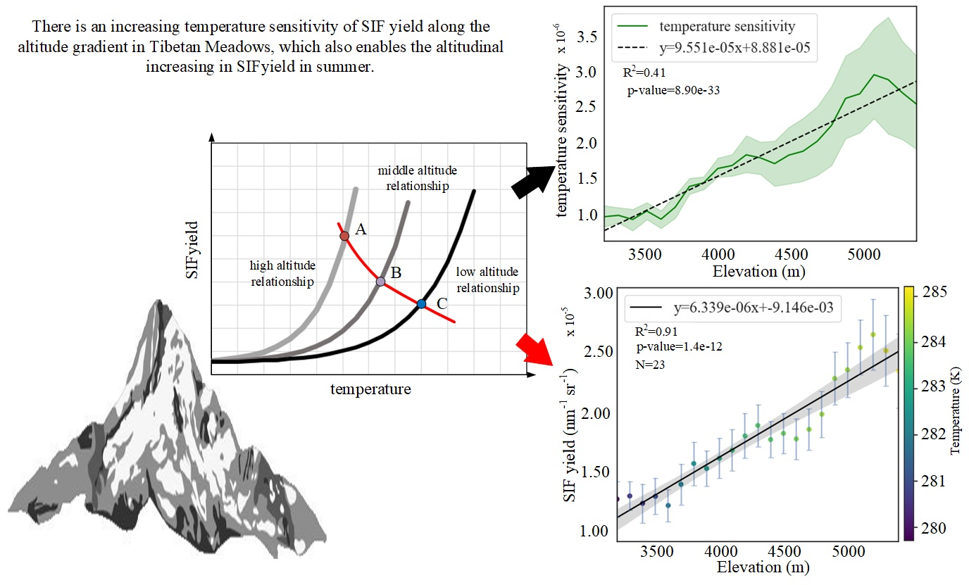
3.2. Altitudinal Patterns of Changes in SIFyield Temperature Sensitivity

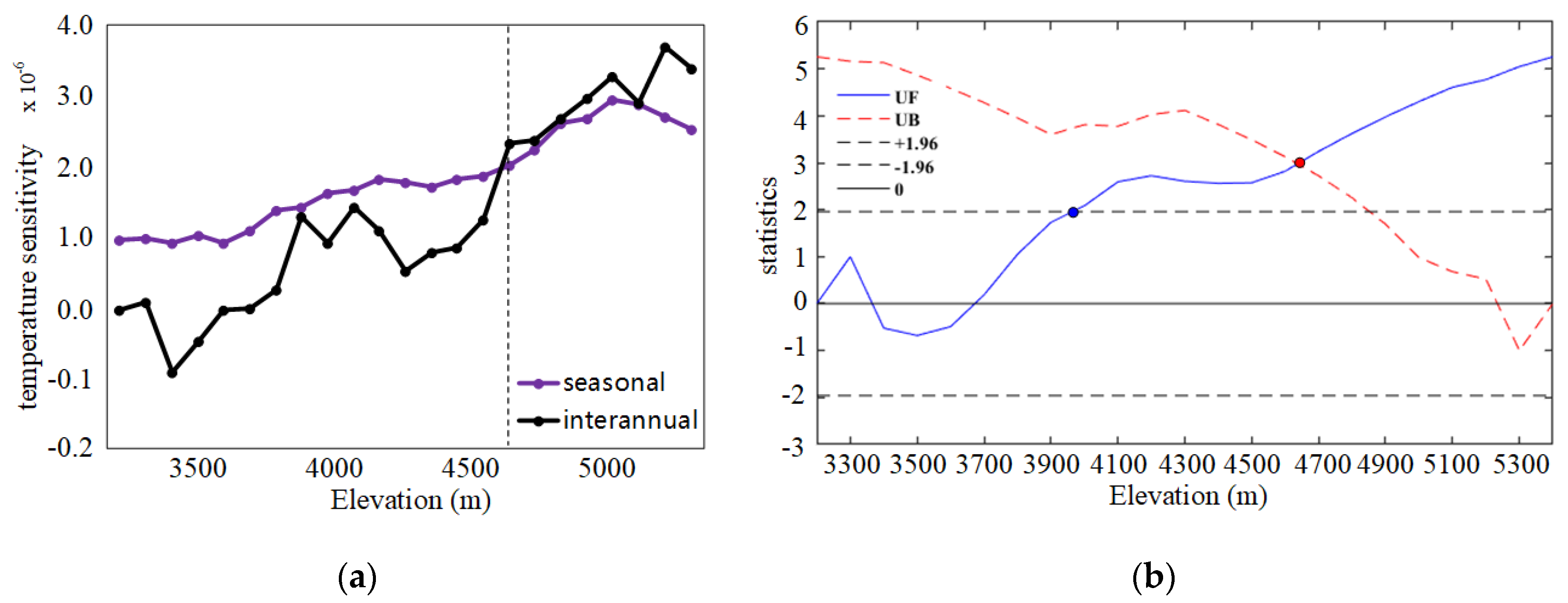
3.2.1. Seasonal and Interannual Temperature Sensitivity of SIFyield

In addition to the altitudinal variation in S I F y i e l d itself, its temperature sensitivity also varies along the altitudinal gradient. The altitudinal variation in seasonal temperature sensitivity is shown in Figure 6a. In spite of increased uncertainty, the temperature sensitivity rises along the altitudinal gradient. When the altitude rises above 5000 m, temperature sensitivity begins to decrease, probably because the plants there are already subnival plants, and the extreme environment there make them different from other alpine plants. Taking the difference between temperature sensitivity at 4900–5000 m and 3200–3300 m as an example, the Wilcoxon rank sum test was conducted to examine the altitudinal differences. According to Figure 6b, there is indeed a significant difference between the averages of temperature sensitivity at high and low altitudes (p < 0.001). The figure also shows a flatter shape of the temperature sensitivity distribution at 4900–5000 m than that at 3200–3300 m, which results from a larger standard deviation (for 3200–3300 m, stdev = 0.001028; for 4900–5000 m, stdev = 0.000278) at higher altitudes.
With regard to interannual variance, the coefficient of determination between temperature sensitivity and altitude is not so large (R2 = 0.41) (Figure 6a), but that of the relationship between multi-year average temperature sensitivity and elevation is fairly high (R2 = 0.93). These results show that elevation itself is enough to explain the altitudinal variation in temperature sensitivity, although there are still latent variables driving the multi-year changes of variation.
When we look into the altitudinal variation in temperature sensitivity in different years (Figure 6d), it can be discovered easily that the interannual differences are significantly enhanced for places above 4200 m. Except for 2018, it seems that years with large seasonal temperature sensitivity in high altitude regions, for example 2008, 2011, and 2013, usually had relatively high S I F y i e l d , and years with small seasonal temperature sensitivity, such as 2015, had low S I F y i e l d .
Besides the seasonal scale, temperature sensitivity calculated at the interannual scale also increases as the elevation rises (Figure 6c). Although the coefficient of determination of interannual temperature sensitivity is smaller than that of seasonal temperature sensitivity, its slope is much greater (seasonal: slope = 0.000188 nm−1 sr−1 K−1 m−1; interannual: slope = 0.000096 nm−1 sr−1 K−1 m−1).
Temperature sensitivity at seasonal and interannual scales was further compared, as shown in Figure 7a. In low-altitude regions, interannual temperature sensitivity is lower than seasonal, and when the altitude reaches 4700–4800 m, interannual temperature sensitivity surpasses seasonal. Both seasonal and interannual temperature sensitivity pass the Mann–Kendall test and show a significant increasing trend along the altitude gradient, but an abrupt point is not detected in either of them.

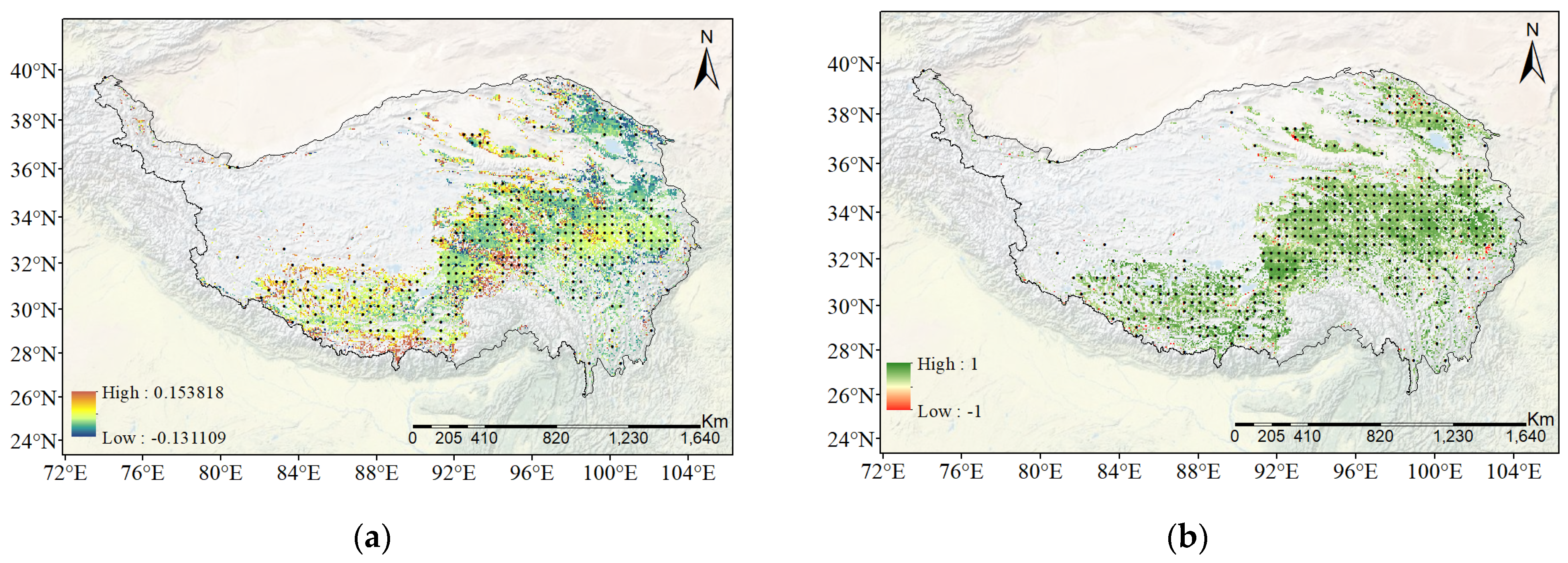
3.2.2. Spatial Distribution of Temperature Sensitivity of SIFyield

The spatial distribution of temperature sensitivity of S I F y i e l d is displayed in Figure 8a, and the spatial distribution of the tau statistic in the Mann–Kendall test is shown in Figure 8b. Figure 8c shows the elevation map of study region, and Figure 8d shows that the alpine kobresia weedy grass meadow is generally the main type of vegetation in Tibetan meadows. The results in Figure 8a,c and d show that regions with high temperature sensitivity are generally at high altitude, even if the vegetations there belong to the same vegetation subtype, which is consistent with the results in Section 3.2.1. Most of the regions have positive tau and small p-value (p-value < 0.1) (Figure 8b), which demonstrates the significant increasing trend of SIFyield as the temperature rises above 275 K.

4. Discussion

4.1. Possible Altitudinal Increase in SIFyield Observed in Summer

The increasing trend of S I F y i e l d along the elevation on summer days can be explained by the altitude-dependent relationship between   S I F y i e l d and environmental variables such as temperature. In addition to the different relationships between S I F y i e l d and air temperature at different altitudes, Figure 4b also shows the altitudinal variation in S I F y i e l d on DOY 205 and 213. From the seasonal results, we can infer that the higher temperature sensitivity at high altitudes makes the altitudinal increase in S I F y i e l d possible on DOY 205 and 213. If the temperature sensitivity at different altitudes stays the same, only the result that S I F y i e l d decreases with altitude (increases with ambient temperature) can be obtained.
The schematic diagrams in Figure 9 show that the difference in sensitivity at different altitudes makes the high S I F y i e l d phenomenon possible at high altitudes. If the altitudinal variation in temperature sensitivity of S I F y i e l d (or its sensitivity to other environmental elements) is not taken into account, as shown in Figure 9a, then it is only possible to conclude that S I F y i e l d is lower at high altitudes, and we cannot obtain results consistent with satellite observations. Therefore, even if S I F y i e l d is found to be higher at higher elevation, it does not necessarily mean that the correlation between temperature and S I F y i e l d is negative for given site observations (Figure 9b).
The varied vegetation along the altitude gradient may also play an important role in the formation of altitudinal S I F y i e l d patterns. Numerous studies report special physiological responses and photosynthetic behaviors of alpine plants, especially in tropical and subtropical regions [17,62]. Previous studies also reported relatively high activity of photosynthesis and its related traits at high altitudes. Ground observation in the eastern Qinghai-Tibetan Plateau found an increase in the maximum carboxylation rate (Vcmax) and maximal electron transport rate (Jmax) along the elevation gradient, indicating higher levels of carbon assimilation and function to cope with the harsh conditions and a shorter growing season for plants at higher elevations [15]. Actually, the increase in Vcmax and drawdown of carbon dioxide (CO2) with increased altitude have been consistently observed for many years and proved by numerous studies [2,4,5,14,63,64,65,66,67]. In addition, equal or even higher photosynthetic rates were also measured [68], and various hypotheses have been proposed to explain this puzzling phenomenon, mainly including theories focusing on low temperatures [5,66,69] and low pressure [70,71]. Optimality principles such as the least-cost hypothesis and coordination hypothesis were also employed in a theoretical model in 2017 [2]. This model successfully simulated increasing Vcmax and decreasing ambient CO2 partial pressure with rising altitude from 0–3000 m. Although a consensus on the mechanism of this phenomenon has not been reached, all of the above findings confirm that there are changes in the properties of the plants themselves along the altitude. These results also demonstrate that there are occasions when photosynthetic capacity increases at higher altitudes, implying there may also be enhancement of other photosynthesis-related traits, such as S I F y i e l d , along the altitude gradient.
In addition, plants in high-altitude places usually suffer from severe excess light stress [16,31], as the light reaction and carbon reaction are prone to be out of sync under conditions of low temperature and high light intensity. As a pathway of energy dissipation [72], fluorescence emission may also be enhanced to dissipate excess light energy. According to studies mentioned above, the differences in the characteristics of vegetation along the altitude gradient, especially traits related to photosynthesis, have shown relatively obvious responses to the environmental conditions in their habitats along the altitude. Therefore, it is possible that SIFyield will rise along the altitude gradient as a strategy to adapt to the environment.

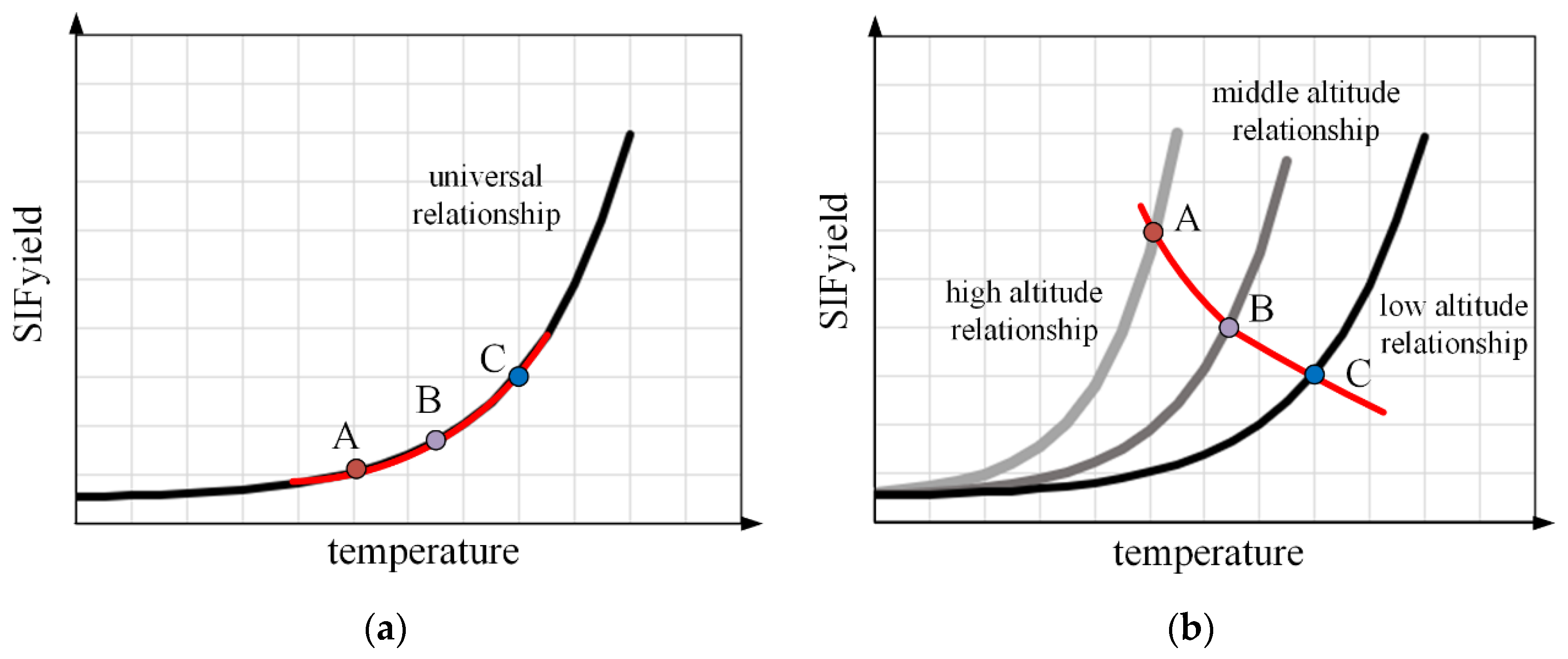
4.2. Interpretation of Patterns Observed at Different Scales

As highlighted by Körner [1], although they are under the umbrella of altitude gradient, vertical variation patterns of vegetation described from different perspectives and in different regions are usually controlled by diverse drivers. Altitude-dependent S I F y i e l d patterns observed at different scales in this study also reflect different issues and involve various latent factors. Therefore, discrepancies in these S I F y i e l d variation patterns do not necessarily represent a contradiction.
S I F y i e l d patterns discovered on the interannual scale are probably close to analysis results based on controlled experiments. Due to the similarity of seasonal cycle phases on the same DOY across years, the influence of growth stages, incident solar energy, and other corresponding environmental variables driven by seasonal cycles is diminished on the interannual scale. In this case, the contribution of environmental changes (temperature and PAR) to S I F y i e l d variation is enhanced and accentuated, and the results obtained from this perspective are relatively independent of some common factors in seasonal cycles. Therefore, interannual patterns of S I F y i e l d might reflect the response of photosynthesis-related physiological activity of plants in a given place. The stable negative correlation between S I F y i e l d and PAR on different DOYs discovered on the interannual scale (Figure 5a) is consistent with previous ground observations showing a negative impact of PAR on S I F y i e l d [73].
In comparison with the pattern above, S I F y i e l d variation on the seasonal scale reflects the mixed effects of seasonal variables on photosynthesis-related vegetation activity. The formation of this phenomenon involves entangled covariations of different variables. Thus, it is reasonable that they would be different from interannual results. Peaks of S I F y i e l d at different altitudes occur in summer, which is also the peak time of vegetation activity. The S I F y i e l d at all altitudes increases with rising temperature at this scale, which is consistent with the increased fluorescence yield and non-photosynthetic quenching (NPQ) discovered at a high-elevation evergreen forest in summer [74].
To summarize, patterns in this study actually indicate the different responses of vegetation to environmental changes along the altitude at seasonal and interannual scales. The altitudinal variation in S I F y i e l d may result from natural selection at the ecosystem scale. It involves the adaptation of plants to long-lasting environmental stresses in their habitats and actually reflects the long-term response of plants to environmental changes [1]. Actually, photosynthetic capacity is considered to be one of the ways the adaptation mechanism and survival strategies work for alpine plants on the Tibetan Plateau [75]. Change on the seasonal scale may be the result of long-term cyclically changing environmental conditions involving the influence of seasonal cycles. The variation in seasonal patterns at different altitudes may be related to phenological issues, indicating the adaptation of plants to the harsh environmental condition and the short growing season at high altitudes [15]. In contrast, the patterns on the interannual scale reflect the shortest-term response of S I F y i e l d to environmental changes in the absence of plant adaptation, which is similar to the condition of global changes when there is not enough time for plants to develop and adjust to the changing climate. In other words, the interannual pattern is the response of plants to the environment without considering their adaptation, while their adaptation possibly interferes with seasonal patterns and altitudinal variations. Therefore, all of the patterns are, in a broad sense, the response of vegetation to environmental changes, but the mechanisms behind them are actually different.

5. Conclusions

Based on GOME-2 SIF observations, we inspected variations in SIFyield and its temperature sensitivity along the altitude gradient in Tibetan meadows. First, accompanied by lower air temperature and higher light intensity, SIFyield was found to increase with altitude on summer days, and increased SIFyield during seasonal cycles usually coincides with higher air temperatures. Second, no significant altitudinal differences were found in seasonal SIFyield variations with DOY, whereas the increasing trend of its temperature sensitivity along the elevation gradient was fairly noticeable. Third, a relatively stable and highly negative correlation between SIFyield and PAR was found at the interannual scale, which is consistent with intensified light stress reported in previous studies. Finally, both interannual and seasonal temperature sensitivity increased at high altitudes, the former faster than the latter along the altitude gradient, which even exceeded the seasonal temperature sensitivity above 4700 m. The sensitive response to the changing environment in high-altitude regions implies an urgent need to pay greater attention to alpine vegetation–climate interactions, and the patterns shown in this study may help to advance the understanding of photosynthesis-related physiological activities there.

Author Contributions

Conceptualization, L.L. and R.C.; methodology, L.L. and R.C.; software, R.C.; writing—original draft preparation, R.C.; writing—review and editing, L.L. and X.L.; visualization, R.C.; project administration, L.L. All authors have read and agreed to the published version of the manuscript.

Funding

This research was supported by the National Key Research and Development Program of China (2017YFA0603001), the National Natural Science Foundation of China (41825002), and the Key Research Program of the Chinese Academy of Sciences (ZDRW-ZS-2019-1)

Institutional Review Board Statement

Not applicable.

Informed Consent Statement

Not applicable.

Data Availability Statement

The SIF dataset used in this study comes from the Global degradation corrected 0.05 degree GOME-2 SIF datasets (derived from PK datasets) [50] shared in Zenodo. http://0-doi-org.brum.beds.ac.uk/10.5281/zenodo.4050960 (accessed on 26 September 2020) 8-day instrument degradation corrected 0.05 degree GOME-2 SIF datasets on a global scale from 2010 to 2018. PK dataset from the spatially downscaled sun-induced fluorescence global product proposed by Gregory Duveiller in 2020 is corrected based on a pseudo-invariant method and then masked. Mean value composite method is used to produce monthly data.

Conflicts of Interest

The authors declare no conflict of interest.

References

  1. Körner, C. The use of “altitude” in ecological research. Trends Ecol. Evol. 2007, 22, 569–574. [Google Scholar] [CrossRef] [PubMed]
  2. Wang, H.; Prentice, I.C.; Davis, T.W.; Keenan, T.F.; Wright, I.J.; Peng, C. Photosynthetic responses to altitude: An explanation based on optimality principles. New Phytol. 2017, 213, 976–982. [Google Scholar] [CrossRef] [PubMed] [Green Version]
  3. Wang, S.W.; He, X.F.; Chen, J.G.; Sun, H.; Körner, C.; Yang, Y. Elevation-specific responses of phenology in evergreen oaks from their low-dry to their extreme high-cold range limits in the SE Himalaya. Alp. Bot. 2021. [Google Scholar] [CrossRef]
  4. Gale, J. Availability of carbon dioxide for photosynthesis at high altitudes: Theoretical considerations. Ecology 1972, 53, 494–497. [Google Scholar] [CrossRef]
  5. Friend, A.D.; Woodward, F.I.; Switsur, V.R. Field measurements of photosynthesis, stomatal conductance, leaf nitrogen and δ 13 C along altitudinal gradients in Scotland. Funct. Ecol. 1989, 117–122. [Google Scholar] [CrossRef]
  6. Friend, A.D.; Woodward, F.I. Evolutionary and ecophysiological responses of mountain plants to the growing season environment. In Advances in Ecological Research; Elsevier: Amsterdam, The Netherlands, 1990; Volume 20, pp. 59–124. [Google Scholar]
  7. Machino, S.; Nagano, S.; Hikosaka, K. The latitudinal and altitudinal variations in the biochemical mechanisms of temperature dependence of photosynthesis within Fallopia japonica. Environ. Exp. Bot. 2021, 181, 104248. [Google Scholar] [CrossRef]
  8. Liu, L.; Liu, L.; Liang, L.; Donnelly, A.; Park, I.; Schwartz, M.D. Effects of elevation on spring phenological sensitivity to temperature in Tibetan Plateau grasslands. Chin. Sci. Bull. 2014, 59, 4856–4863. [Google Scholar] [CrossRef]
  9. Luo, T.; Luo, J.; Pan, Y. Leaf traits and associated ecosystem characteristics across subtropical and timberline forests in the Gongga Mountains, Eastern Tibetan Plateau. Oecologia 2005, 142, 261–273. [Google Scholar] [CrossRef]
  10. Buchner, O.; Neuner, G. Variability of heat tolerance in alpine plant species measured at different altitudes. Arctic Antarct. Alp. Res. 2003, 35, 411–420. [Google Scholar] [CrossRef] [Green Version]
  11. Ma, W.; Shi, P.; Li, W.; He, Y.; Zhang, X.; Shen, Z.; Chai, S. Changes in individual plant traits and biomass allocation in alpine meadow with elevation variation on the Qinghai-Tibetan Plateau. Sci. China Life Sci. 2010. [Google Scholar] [CrossRef]
  12. Luo, T.; Brown, S.; Pan, Y.; Shi, P.; Ouyang, H.; Yu, Z.; Zhu, H. Root biomass along subtropical to alpine gradients: Global implication from Tibetan transect studies. For. Ecol. Manag. 2005, 206, 349–363. [Google Scholar] [CrossRef]
  13. Pellissier, L.; Fournier, B.; Guisan, A.; Vittoz, P. Plant traits co-vary with altitude in grasslands and forests in the European Alps. Plant Ecol. 2010. [Google Scholar] [CrossRef] [Green Version]
  14. Peng, Y.; Bloomfield, K.J.; Prentice, I.C. A theory of plant function helps to explain leaf-trait and productivity responses to elevation. New Phytol. 2020. [Google Scholar] [CrossRef]
  15. Wu, J.M.; Shi, Z.; Liu, S.; Centritto, M.; Cao, X.; Zhang, M.; Zhao, G. Photosynthetic capacity of male and female Hippophae rhamnoides plants along an elevation gradient in eastern Qinghai-Tibetan Plateau, China. Tree Physiol. 2020. [Google Scholar] [CrossRef] [PubMed]
  16. García-Plazaola, J.I.; Rojas, R.; Christie, D.A.; Coopman, R.E. Photosynthetic responses of trees in high-elevation forests: Comparing evergreen species along an elevation gradient in the Central Andes. AoB Plants 2015, 7, 1–13. [Google Scholar] [CrossRef] [PubMed] [Green Version]
  17. Streb, P.; Shang, W.; Feierabend, J.; Bligny, R. Divergent strategies of photoprotection in high-mountain plants. Planta 1998, 207, 313–324. [Google Scholar] [CrossRef]
  18. Schimel, D.; Pavlick, R.; Fisher, J.B.; Asner, G.P.; Saatchi, S.; Townsend, P.; Miller, C.; Frankenberg, C.; Hibbard, K.; Cox, P. Observing terrestrial ecosystems and the carbon cycle from space. Glob. Chang. Biol. 2015, 21, 1762–1776. [Google Scholar] [CrossRef]
  19. Frankenberg, C.; Fisher, J.B.; Worden, J.; Badgley, G.; Saatchi, S.S.; Lee, J.E.; Toon, G.C.; Butz, A.; Jung, M.; Kuze, A.; et al. New global observations of the terrestrial carbon cycle from GOSAT: Patterns of plant fluorescence with gross primary productivity. Geophys. Res. Lett. 2011. [Google Scholar] [CrossRef] [Green Version]
  20. Joiner, J.; Guanter, L.; Lindstrot, R.; Voigt, M.; Vasilkov, A.P.; Middleton, E.M.; Huemmrich, K.F.; Yoshida, Y.; Frankenberg, C. Global monitoring of terrestrial chlorophyll fluorescence from moderate-spectral-resolution near-infrared satellite measurements: Methodology, simulations, and application to GOME-2. Atmos. Meas. Tech. 2013, 6, 2803–2823. [Google Scholar] [CrossRef] [Green Version]
  21. Guanter, L.; Frankenberg, C.; Dudhia, A.; Lewis, P.E.; Gómez-Dans, J.; Kuze, A.; Suto, H.; Grainger, R.G. Retrieval and global assessment of terrestrial chlorophyll fluorescence from GOSAT space measurements. Remote Sens Environ. 2012. [Google Scholar] [CrossRef]
  22. Joiner, J.; Yoshida, Y.; Vasilkov, A.P.; Yoshida, Y.; Corp, L.A.; Middleton, E.M. First observations of global and seasonal terrestrial chlorophyll fluorescence from space. Biogeosciences 2011. [Google Scholar] [CrossRef] [Green Version]
  23. Köhler, P.; Guanter, L.; Joiner, J. A linear method for the retrieval of sun-induced chlorophyll fluorescence from GOME-2 and SCIAMACHY data. Atmos. Meas. Tech. 2015, 8, 2589–2608. [Google Scholar] [CrossRef] [Green Version]
  24. Köhler, P.; Frankenberg, C.; Magney, T.S.; Guanter, L.; Joiner, J.; Landgraf, J. Global retrievals of solar-induced chlorophyll fluorescence with TROPOMI: First results and intersensor comparison to OCO-2. Geophys. Res. Lett. 2018, 45, 10456–10463. [Google Scholar] [CrossRef] [Green Version]
  25. Guanter, L.; Alonso, L.; Gómez-Chova, L.; Amorós-López, J.; Vila, J.; Moreno, J. Estimation of solar-induced vegetation fluorescence from space measurements. Geophys. Res. Lett. 2007. [Google Scholar] [CrossRef]
  26. Wang, C.; Guan, K.; Peng, B.; Chen, M.; Jiang, C.; Zeng, Y.; Wu, G.; Wang, S.; Wu, J.; Yang, X.; et al. Satellite footprint data from OCO-2 and TROPOMI reveal significant spatio-temporal and inter-vegetation type variabilities of solar-induced fluorescence yield in the US Midwest. Remote Sens. Environ. 2020, 241, 111728. [Google Scholar] [CrossRef]
  27. Wang, X.; Qiu, B.; Li, W.; Zhang, Q. Impacts of drought and heatwave on the terrestrial ecosystem in China as revealed by satellite solar-induced chlorophyll fluorescence. Sci. Total Environ. 2019, 693, 133627. [Google Scholar] [CrossRef] [PubMed]
  28. Song, L.; Guanter, L.; Guan, K.; You, L.; Huete, A.; Ju, W.; Zhang, Y. Satellite sun-induced chlorophyll fluorescence detects early response of winter wheat to heat stress in the Indian Indo-Gangetic Plains. Glob. Chang. Biol. 2018, 24, 4023–4037. [Google Scholar] [CrossRef] [Green Version]
  29. Pepin, N.C.; Lundquist, J.D. Temperature trends at high elevations: Patterns across the globe. Geophys. Res. Lett. 2008, 35. [Google Scholar] [CrossRef] [Green Version]
  30. Rangwala, I.; Miller, J.R. Climate change in mountains: A review of elevation-dependent warming and its possible causes. Clim. Chang. 2012, 114, 527–547. [Google Scholar] [CrossRef]
  31. Flexas, J.; Loreto, F.; Medrano, H. Terrestrial Photosynthesis in a Changing Environment: A Molecular, Physiological, and Ecological Approach; Cambridge University Press: Cambridge, UK, 2012. [Google Scholar]
  32. Barber, J.; Andersson, B. Too much of a good thing: Light can be bad for photosynthesis. Trends Biochem. Sci. 1992, 17, 61–66. [Google Scholar] [CrossRef]
  33. Ball, M.C.; Hodges, V.S.; Laughlin, G.P. Cold-induced photoinhibition limits regeneration of snow gum at tree-line. Funct. Ecol. 1991, 663–668. [Google Scholar] [CrossRef]
  34. Ensminger, I.; Busch, F.; Huner, N.P.A. Photostasis and cold acclimation: Sensing low temperature through photosynthesis. Physiol. Plant. 2006, 126, 28–44. [Google Scholar] [CrossRef]
  35. Huner, N.P.A.; Öquist, G.; Sarhan, F. Energy balance and acclimation to light and cold. Trends Plant Sci. 1998, 3, 224–230. [Google Scholar] [CrossRef]
  36. Cannone, N.; Sgorbati, S.; Guglielmin, M. Unexpected impacts of climate change on alpine vegetation. Front. Ecol. Environ. 2007, 5, 360–364. [Google Scholar] [CrossRef] [Green Version]
  37. Grabherr, G.; Gottfried, M.; Pauli, H. Climate change impacts in alpine environments. Geogr. Compass 2010, 4, 1133–1153. [Google Scholar] [CrossRef] [Green Version]
  38. Duan, A.; Xiao, Z. Does the climate warming hiatus exist over the Tibetan Plateau? Sci. Rep. 2015, 5, 13711. [Google Scholar] [CrossRef]
  39. Liu, X.; Chen, B. Climatic warming in the Tibetan Plateau during recent decades. Int. J. Climatol. J. R. Meteorol. Soc. 2000, 20, 1729–1742. [Google Scholar] [CrossRef]
  40. Zhang, R.; Jiang, D.; Zhang, Z.; Yu, E. The impact of regional uplift of the Tibetan Plateau on the Asian monsoon climate. Palaeogeogr. Palaeoclimatol. Palaeoecol. 2015, 417, 137–150. [Google Scholar] [CrossRef]
  41. Liu, X.; Yin, Z.-Y. Sensitivity of East Asian monsoon climate to the uplift of the Tibetan Plateau. Palaeogeogr. Palaeoclimatol. Palaeoecol. 2002, 183, 223–245. [Google Scholar] [CrossRef] [Green Version]
  42. Liu, X.; Kutzbach, J.E.; Liu, Z.; An, Z.; Li, L. The Tibetan Plateau as amplifier of orbital-scale variability of the East Asian monsoon. Geophys. Res. Lett. 2003, 30. [Google Scholar] [CrossRef] [Green Version]
  43. Harris, N. The elevation history of the Tibetan Plateau and its implications for the Asian monsoon. Palaeogeogr. Palaeoclimatol. Palaeoecol. 2006, 241, 4–15. [Google Scholar] [CrossRef]
  44. Kang, S.; Xu, Y.; You, Q.; Flügel, W.-A.; Pepin, N.; Yao, T. Review of climate and cryospheric change in the Tibetan Plateau. Environ. Res. Lett. 2010, 5, 15101. [Google Scholar] [CrossRef]
  45. Harris, R.B. Rangeland degradation on the Qinghai-Tibetan plateau: A review of the evidence of its magnitude and causes. J. Arid. Environ. 2010, 74, 1–12. [Google Scholar] [CrossRef]
  46. Fang, X.; Han, Y.; Ma, J.; Song, L.; Yang, S.; Zhang, X. Dust storms and loess accumulation on the Tibetan Plateau: A case study of dust event on 4 March 2003 in Lhasa. Chin. Sci. Bull. 2004, 49, 953–960. [Google Scholar] [CrossRef]
  47. Duveiller, G.; Filipponi, F.; Walther, S.; Köhler, P.; Frankenberg, C.; Guanter, L.; Cescatti, A. A spatially downscaled sun-induced fluorescence global product for enhanced monitoring of vegetation productivity. Earth Syst. Sci. Data 2020, 12, 1101–1116. [Google Scholar] [CrossRef]
  48. Joiner, J.; Yoshida, Y.; Guanter, L.; Middleton, E.M. New methods for retrieval of chlorophyll red fluorescence from hyper-spectral satellite instruments: Simulations and application to GOME-2 and SCIAMACHY. Atmos. Meas. Tech. Discuss. 2016. [Google Scholar] [CrossRef] [Green Version]
  49. Zhang, Y.; Joiner, J.; Gentine, P.; Zhou, S. Reduced solar-induced chlorophyll fluorescence from GOME-2 during Amazon drought caused by dataset artifacts. Glob. Chang. Biol. 2018, 24, 2229–2230. [Google Scholar] [CrossRef] [PubMed] [Green Version]
  50. Liangyun, L.; Yan, M.; Ruonan, C. Global degradation corrected 0.05 degree GOME-2 SIF datasets (derived from PK datasets) [Dataset]. Zenodo 2020. [Google Scholar] [CrossRef]
  51. He, J.; Yang, K.; Tang, W.; Lu, H.; Qin, J.; Chen, Y.Y.; Li, X. The first high-resolution meteorological forcing dataset for land process studies over China. Sci. Data 2020, 7, 25. [Google Scholar] [CrossRef] [Green Version]
  52. Yang, K.; He, J.; Tang, W.J.; Qin, J.; Cheng, C.C.K. On downward shortwave and longwave radiations over high altitude regions: Observation and modeling in the Tibetan Plateau. Agric. For. Meteorol. 2010, 150, 38–46. [Google Scholar] [CrossRef]
  53. Jarvis, A.; Reuter, H.I.; Nelson, A.; Guevara, E. Guevara, 2008, Hole-filled seamless SRTM data V4. International Centre for Tropical Agriculture (CIAT). Available online: http://srtm.csi.cgiar.org (accessed on 1 September 2020).
  54. Reuter, H.I.; Nelson, A.; Jarvis, A. An evaluation of void filling interpolation methods for SRTM data. Int. J. Geogr. Inf. Sci. 2007, 21, 983–1008. [Google Scholar] [CrossRef]
  55. Zhang, Y.L.; Li, B.Y.; Zheng, D. Datasets of the Boundary and Area of the Tibetan Plateau [DB/OL]. Glob. Chang. Data Repos. 2014. [Google Scholar] [CrossRef]
  56. Xiao, Z.; Liang, S.; Sun, R.; Wang, J.; Jiang, B. Estimating the fraction of absorbed photosynthetically active radiation from the MODIS data based GLASS leaf area index product. Remote Sens. Environ. 2015, 171, 105–117. [Google Scholar] [CrossRef]
  57. Xiao, Z.; Liang, S.; Sun, R. Evaluation of three long time series for global fraction of absorbed photosynthetically active radiation (fapar) products. IEEE Trans. Geosci. Remote Sens. 2018, 56, 5509–5524. [Google Scholar] [CrossRef]
  58. Editorial Committee of the Chinese Vegetation Map of the Chinese Academy of Sciences. 1980 1:1 million vegetation map of China. Institute of Botany, Chinese Academy of Sciences. Available online: http://hdl.pid21.cn/21.86109/casearth.5c19a5680600cf2a3c557b6b (accessed on 1 September 2020).
  59. Guanter, L.; Zhang, Y.; Jung, M.; Joiner, J.; Voigt, M.; Berry, J.A.; Frankenberg, C.; Huete, A.R.; Zarco-Tejada, P.; Lee, J.E.; et al. Global and time-resolved monitoring of crop photosynthesis with chlorophyll fluorescence. Proc. Natl. Acad. Sci. USA 2014, 111. [Google Scholar] [CrossRef] [PubMed] [Green Version]
  60. Mann, H.B. Nonparametric Tests Against Trend. Econometrica 1945. [Google Scholar] [CrossRef]
  61. Bevan, J.M.; Kendall, M.G. Rank Correlation Methods. J. R. Stat. Soc. 1971. [Google Scholar] [CrossRef]
  62. Magaña Ugarte, R.; Escudero, A.; Gavilán, R.G. Metabolic and physiological responses of Mediterranean high-mountain and alpine plants to combined abiotic stresses. Physiol Plant. 2019, 165, 403–412. [Google Scholar] [CrossRef]
  63. Terashima, I.; Masuzawa, T.; Ohba, H.; Yokoi, Y. Is photosynthesis suppressed at higher elevations due to low CO2 pressure? Ecology 1995, 76, 2663–2668. [Google Scholar] [CrossRef]
  64. Bresson, C.C.; Kowalski, A.S.; Kremer, A.; Delzon, S. Evidence of altitudinal increase in photosynthetic capacity: Gas exchange measurements at ambient and constant CO2 partial pressures. Ann. For. Sci. 2009, 66, 1–8. [Google Scholar] [CrossRef] [Green Version]
  65. Zhu, Y.; Siegwolf, R.T.W.; Durka, W.; Körner, C. Phylogenetically balanced evidence for structural and carbon isotope responses in plants along elevational gradients. Oecologia 2010, 162, 853–863. [Google Scholar] [CrossRef] [PubMed]
  66. Korner, C.; Diemer, M. In situ photosynthetic responses to light, temperature and carbon dioxide in herbaceous plants from low and high altitude. Funct. Ecol. 1987, 179–194. [Google Scholar] [CrossRef]
  67. Reed, C.C.; Loik, M.E. Water relations and photosynthesis along an elevation gradient for Artemisia tridentata during an historic drought. Oecologia 2016, 181, 65–76. [Google Scholar] [CrossRef] [PubMed] [Green Version]
  68. Shi, Z.; Liu, S.; Liu, X.; Centritto, M. Altitudinal variation in photosynthetic capacity, diffusional conductance and δ13C of butterfly bush (Buddleja davidii) plants growing at high elevations. Physiol Plant. 2006, 128, 722–731. [Google Scholar] [CrossRef]
  69. Vitousek, P.M.; Field, C.B.; Matson, P.A. Variation in foliar δ 13 C in Hawaiian Metrosideros polymorpha: A case of internal resistance? Oecologia 1990, 84, 362–370. [Google Scholar] [CrossRef] [PubMed]
  70. Decker, J.P. Some effects of temperature and carbon dioxide concentration on photosynthesis of Mimulus. Plant Physiol. 1959, 34, 103. [Google Scholar] [CrossRef] [Green Version]
  71. Billings, W.D.; Clebsch, E.E.C.; Mooney, H.A. Effect of low concentrations of carbon dioxide on photosynthesis rates of two races of Oxyria. Science 1961, 133, 1834. [Google Scholar] [CrossRef]
  72. Porcar-Castell, A.; Tyystjärvi, E.; Atherton, J.; Van der Tol, C.; Flexas, J.; Pfündel, E.E.; Moreno, J.; Frankenberg, C.; Berry, J.A. Linking chlorophyll a fluorescence to photosynthesis for remote sensing applications: Mechanisms and challenges. J. Exp. Bot. 2014, 65, 4065–4095. [Google Scholar] [CrossRef]
  73. Nichol, C.J.; Drolet, G.; Porcar-Castell, A.; Wade, T.; Sabater, N.; Middleton, E.M.; MacLellan, C.; Levula, J.; Mammarella, I.; Vesala, T. Diurnal and seasonal solar induced chlorophyll fluorescence and photosynthesis in a boreal scots pine canopy. Remote Sens. 2019, 11, 273. [Google Scholar] [CrossRef] [Green Version]
  74. Raczka, B.; Porcar-Castell, A.; Magney, T.; Lee, J.E.; Köhler, P.; Frankenberg, C.; Grossmann, K.; Logan, B.A.; Stutz, J.; Blanken, P.D.; et al. Sustained Nonphotochemical Quenching Shapes the Seasonal Pattern of Solar-Induced Fluorescence at a High-Elevation Evergreen Forest. J. Geophys. Res. Biogeosci. 2019, 124, 2005–2020. [Google Scholar] [CrossRef]
  75. Cui, G.; Ji, G.; Liu, S.; Li, B.; Lian, L.; He, W.; Zhang, P. Physiological adaptations of Elymus dahuricus to high altitude on the Qinghai–Tibetan Plateau. Acta Physiol. Plant. 2019, 41, 1–9. [Google Scholar] [CrossRef]
Figure 1. Variations in S I F y i e l d along altitudinal gradient. (a) Altitudinal S I F y i e l d variation on day of year (DOY) 197 (July, the peak of summer growth period); (b) S I F y i e l d changes along altitude in 12 years on DOY 197 (July, the peak of summer growth period). Graph (a) is derived from the average of 12-year observations, while (b) shows altitudinal effects on S I F y i e l d and SIF in each year from 2007–2018. Colors in (a) represent the temperature of ambient environment, and colors in (b) represent year; shaded areas represent the 95% confidence interval Error bars in (a) represent the standard error of S I F y i e l d at different altitudes.
Remotesensing 13 01400 g001
Figure 2. S I F y i e l d changes from 2007–2018 at different elevations. Results are derived from SIF observations on (a) DOY 197 (July, the peak of summer growth period) and (b) DOY 149 (May, regreening period at late spring). 3.1.2. Altitude-Dependent SIFyield Changes at Seasonal Scale.
Remotesensing 13 01400 g002
Figure 3. Seasonal variations in (a) SIF, (b) S I F y i e l d , (c) photosynthetically active radiation (PAR), and (d) temperature at different elevations. Lines in each subgraph indicate DOY when variables reach their peaks, and gray rectangles indicate S I F y i e l d peak time for comparison.
Remotesensing 13 01400 g003
Figure 4. Temperature responses of (a) SIF and (b) S I F y i e l d at different altitudes at seasonal scales. Observations from DOY 93 (April, early regreening period at late spring), 133 (May, early regreening period at late spring), 205 (July, the peak of summer growth period), and 213 (August, the late summer growth period) are marked.
Remotesensing 13 01400 g004
Figure 5. (a) Variations in R2 between SIFyield and environmental variables (PAR and temperature). Observations from DOY 133–277 are used. Color of bars indicates direction of correlation (red indicates positive and blue indicates negative); deeper color indicates higher R2. (b) Relationship between SIFyield and PAR at different elevations on DOY 205 (July, the peak of summer growth period).
Remotesensing 13 01400 g005
Figure 6. (a) Seasonal temperature sensitivity along altitudinal gradient, derived from annual cycle. (b) Distribution of temperature sensitivity at 4900–5000 m (in blue) and 3200–3300 m (in gray), showing significant differences between them. (c) Interannual temperature sensitivity along altitudinal gradient; different from results in Figure 5a, temperature sensitivity calculated here does not distinguish differences in DOYs, and shows a generally positive relationship between S I F y i e l d and temperature (positive temperature sensitivity) at interannual scale in most regions. (d) Altitudinal variation in temperature sensitivity in different years. Shaded areas represent the 95% confidence interval and the unit of temperature sensitivity is nm−1 sr−1 K−1.
Remotesensing 13 01400 g006
Figure 7. (a) Altitudinal variation in temperature sensitivity at seasonal and interannual scale. (b) Mann–Kendall test result of interannual temperature sensitivity along altitude gradient; no abrupt point was detected. Red dots indicate abrupt points of temperature sensitivity; blue dots indicate altitude threshold of significant increase in temperature sensitivity. Unit of temperature sensitivity is nm−1 sr−1 K−1.
Remotesensing 13 01400 g007
Figure 8. (a) Spatial distribution of seasonal temperature sensitivity of SIFyield; (b) spatial distribution of tau statistic in Mann–Kendall test. Dots indicate significance of regression or Mann–Kendall test (p-value < 0.05). (c) Elevations of study region (data source: STRM-DEM); (d) spatial distribution of vegetation subtypes of Tibetan meadows (data source: vegetation map provided by the Institute of Botany, Chinese Academy of Sciences). Only regions recognized as meadows are displayed in these maps.
Remotesensing 13 01400 g008aRemotesensing 13 01400 g008b
Figure 9. Schematic diagrams showing that temperature sensitivity makes high S I F y i e l d at high altitudes possible. (a) Altitudinal patterns of S I F y i e l d when there is no altitudinal variation of temperature sensitivity. (b) Possible altitudinal patterns of S I F y i e l d when accounting for altitudinal variation of temperature sensitivity. A, B, and C represent regions from high to low altitude, corresponding to temperature variation from low to high.
Remotesensing 13 01400 g009
Publisher’s Note: MDPI stays neutral with regard to jurisdictional claims in published maps and institutional affiliations.

