Applications of Satellite Radar Imagery for Hazard Monitoring: Insights from Australia

Abstract

Earth observation (EO) satellites facilitate hazard monitoring and mapping over large-scale and remote areas. Despite Synthetic Aperture Radar (SAR) satellites being well-documented as a hazard monitoring tool, the uptake of these data is geographically variable, with the Australian continent being one example where the use of SAR data is limited. Consequently, less is known about how these data apply in the Australian context, how they could aid national hazard monitoring and assessment, and what new insights could be gleaned for the benefit of the international disaster risk reduction community. The European Space Agency Sentinel-1 satellite mission now provides the first spatially and temporally complete global SAR dataset and the first opportunity to use these data to systematically assess hazards in new locations. Using the example of Australia, where floods and uncontrolled bushfires, earthquakes, resource extraction (groundwater, mining, hydrocarbons) and geomorphological changes each pose potential risks to communities, we review past usage of EO for hazard monitoring and present a suite of new case studies that demonstrate the potential added benefits of SAR. The outcomes provide a baseline understanding of the potential role of SAR in national hazard monitoring and assessment in an Australian context. Future opportunities to improve national hazard identification will arise from: new SAR sensing capabilities, which for Australia includes a first-ever civilian EO capability, NovaSAR-1; the integration of Sentinel-1 SAR with other EO datasets; and the provision of standardised SAR products via Analysis Ready Data and Open Data Cubes to support operational applications.

1. Introduction

Hazards may be defined as any “process, phenomenon or human activity that may cause loss of life, injury or other health impacts, property damage, social and economic disruption or environmental degradation” [1]. Hazard identification, assessment, and monitoring is a keystone of disaster risk reduction activities, and space-based Earth Observation (EO) data, including from Synthetic Aperture Radar (SAR), are well-documented to be valuable tools for monitoring, mapping, and characterizing natural and man-made hazards.

Globally, Australia is one of the largest users (by volume and variety) of EO data derived from satellites [2], with EO contributing to national hazard monitoring and response [3] and over 100 state and federal government programs. As such, Australia is playing a leading role in global efforts for the provision of operational standardised EO datasets (i.e., Analysis Ready Data), including through Open Data Cube initiatives such as Digital Earth Australia (DEA: [4]; http://www.ga.gov.au/dea; accessed on 16 March 2021). Despite this well-established and extensive use of EO data across multiple sectors, Australian uptake of data from SAR satellites (for hazard monitoring or other purposes) is limited. Therefore, despite the advantages of using these data for hazard assessment (described throughout this study), less is known about how these data apply in the Australian context and how they could aid in national hazard identification and monitoring.

Major factors contributing to the limited uptake of SAR include: the limited spatial and temporal coverage of open-access datasets, which, for Australia, historically offered few consistent (20 images or more e.g., [5]) time-series (see Figure 1 for the example of the European Space Agency’s ENVISAT ASAR, which operated between 2004–2011—refer to Table S2 in the Supplementary Material for further sensor specifications); the cost of commercial datasets; the well-established and successful use of optical/multi-spectral EO data under Australian conditions (e.g., 25 years of archived Landsat imagery used to map continental-scale variations of surface water: [6]); and a subsequent lack of proven SAR applications or expertise, hindering support in industry and government (e.g., [7]).

Significantly, the European Space Agency SAR satellite constellation, Sentinel-1, has now consistently imaged the whole Australian continent since 2016 (Figure 1), presenting the first opportunity to implement SAR as a systematic hazard-monitoring tool on a national scale. Simultaneously Australia’s federal scientific research agency (Commonwealth Science and Industrial Research Organisation–CSIRO) has also secured fractional ownership over tasking of the UK-owned and operated SAR satellite NovaSAR-1 [8], marking Australia’s first-ever civilian EO capability [9].

In response to these step-changes in data availability and the ongoing need to improve hazard monitoring, here we review past usage of SAR for hazard assessment in the context of Australia and use a suite of new case studies to scope the potential of these data to enhance national hazard-monitoring efforts. In Section 2, we begin by providing a brief overview of SAR for hazard monitoring in the context of the applications described in this paper (supported by further resources for non-specialist readers in Table S1 and information about SAR sensors in Table S2, Supplementary Material). Section 3, Section 4, Section 5, Section 6 and Section 7 detail the applications identified to be of key significance for Australia (hydrological hazards; fire; natural resource extraction; seismic hazards; geomorphological changes) and summarise the past use of SAR based upon available case studies documented in the scientific literature and publicly available reports. For these applications, we also present new case studies (see Figure 2A for an overview map) that utilise Sentinel-1, plus commercial SAR data (see Table S3 in the Supplementary Material for details of the datasets and processing methods used). Our intentions are: to provide a baseline understanding of the potential role of SAR in national hazard monitoring and assessment in an Australian context; to provide a suite of new case studies that demonstrate SAR applications to a diverse portfolio of hazards that impact Australia and other regions globally; and to highlight opportunities for growth with the current and future influx of data from new SAR satellites (including NovaSAR-1) and other EO data types, plus advances in the provision of standardised SAR products via Analysis Ready Data and Open Data Cubes [10].

2. SAR Sensing of Hazards

In recent decades, SAR has become one of the fastest growing fields of EO and remote sensing (e.g., [11]). SAR is an active remote-sensing technology that operates by illuminating the ground with microwave radiation and recording the reflected response received back at the sensor. Unlike optical EO systems, this means SAR imagery can be acquired in all weathers, through smoke, and at night. A full description of SAR systems, including the effects of imaging geometry and other sources of bias, is beyond the scope of this paper but can be found in [12]. Table S1 in the Supplementary Material also lists key resources for non-specialist readers.

Pixels within SAR images each contain a phase and amplitude component, both of which have applications for detecting, monitoring, and mapping the hazards described in the following sections (Figure 2B). Like optical EO systems, the pixel amplitude, A (often converted to intensity, I, where I = A²), provides information about features and changes on the Earth’s surface. However, the information derived from SAR is complementary to that of optical systems, as A is a function of surface roughness (or structure) and dielectric constant (indicative of moisture and salinity content) that is dependent upon the SAR wavelength. These factors govern the strength and pattern of the backscatter. For example, a flat surface, such as a water body in calm conditions, results in scattering of the incident SAR microwave away from the sensor, thus surface water can be identified by low intensity/amplitude pixel values. For this reason, SAR backscatter intensity thresholding can be used to map surface water coverage dynamics (lakes, rivers, extreme or seasonal floods: Section 3.1). Areas burned during bushfires have also been mapped using temporal variations in backscatter intensity (Section 4).

Backscatter can be interpreted using scattering models to discriminate the most direct wave bounce mechanisms (direct or double-bounce scattering) from complex interactions (volume or surface roughness scattering). Volumetric and other indirect scattering mechanisms can be most efficiently retrieved by using multi-polarized SAR datasets that contain information about the signal phase shifts (e.g., [13]).

The pixel phase is dependent on the summed phase response of all the individual scatterers contained within the resolved area (pixel footprint) on the ground and is essentially random. For phase to be a useful measurement in hazard monitoring, relative phase differences are measured over time, which cancels out the absolute random component. These phase differences are dependent upon the path length between the satellite and Earth’s surface. Variations in pixel phase between multiple SAR images that are acquired over the same region, but at different times (expressed hereafter in yyyymmdd format), can therefore be used to measure mm-to-cm scale displacements of the Earth’s surface, a unique capability of SAR systems compared to other types of EO. This technique, known as Interferometric Synthetic Aperture Radar, or InSAR [14], produces maps of ground displacements called interferograms in the 1D oblique satellite Line-of-Sight (LoS). With only a single LoS geometry, it is not possible to determine, unambiguously, the magnitude of vertical versus horizontal ground motion in the measured InSAR signal unless ground-based geodetic data are available (e.g., [15]) (note that, due to the near-polar orbit of SAR satellite, InSAR measurements are less sensitive to the north-south component of surface displacements). However, if two or more LoS geometries are available from both an ascending (approximately south-to-north) and descending (approximately north-to-south) orbit, then the decomposition of the LoS signals into vertical and horizontal components is possible [16]. InSAR methods have been used to identify precursory behaviour prior to hazardous events (e.g., slow slip prior to landslides: [17]) and to monitor and understand a multitude of natural and human-made hazards (for reviews, see [18,19]). In Australia, this includes subsidence arising from the extraction of resources, such as groundwater (Section 3.2) and hydrocarbons (Section 5), the stability and subsidence of slopes and other structures in open-pit mines (Section 5.2), and earthquakes (Section 6).

If the phase response of scatterers within a pixel varies significantly between images, as expected when fires burn vegetation or floods inundate the land, the phase difference becomes incoherent, causing gaps in interferograms (for further details, see [14]). Mapping spatial and temporal changes in interferometric coherence can therefore be used to map events that cause changes to the surface environment (Figure 2B). Loss of coherence is also caused by large magnitude displacements when the LoS displacement measured across a single pixel exceeds half the sensor wavelength [14]. In these instances, and if the displacement has a component perpendicular to the LoS, it may be possible to use pixel offset tracking to measure larger magnitude displacements (>tens cm) by applying 2D cross-correlation to quantify sub-pixel offsets (e.g., [20]; Figure 2B).

3. Hydrological Hazards

3.1. Flooding

Severe flooding is common in Australia: tropical cyclones impact parts of the country (generally north of −25° S), and the flat topography, particularly along the coasts, results in regular inundation (e.g., [21]). Optical sensors such as MODIS (MODerate Resolution Imaging Spectrometer) provide imagery for flood mapping at 250–1000 m spatial resolution twice daily and have been implemented for operational flood monitoring in Australia (e.g., via the ‘FloodMap’ platform: [22]). However, floods are inherently associated with precipitation and cloud cover that impacts the imaging capability of optical sensors. Therefore, the all-weather, all-time-of-day imaging capability of SAR is advantageous in these conditions, offering observations at significantly higher spatial resolutions (few ms–tens m: Table S2). Open water strongly scatters the SAR wave energy, which usually leads to a contrasty differentiation between water and all other land cover types in SAR images. In addition, long-wavelength SAR (e.g., L-band: ~23 cm: see examples in Table S2) is also able to partially “see” through vegetation, identifying inundation beneath canopy-cover (e.g., [23]) and benefiting hydrodynamic models of flooding in mangroves, wetlands, and other sensitive ecosystems (e.g., [24]).

Despite these advantages, the use of SAR for this purpose in Australia includes only ad hoc validation case studies [22] and international response to large-scale flooding events. The International Charter Space and Major Disasters has been activated by Geoscience Australia in response to tropical cyclones (Queensland: January 2011, February 2015, March 2017) and flash flooding (Lachlan River, New South Wales: 2016). At these times, the Copernicus Emergency Management Service (EMS) and other value-adding agencies have provided additional SAR acquisitions and flood-map products (e.g., the German Aerospace Center automated flood mapping: [25]). Geoscience Australia has also carried out data analysis on request and produced flood maps using simple thresholding of intensity data in single SAR images [26], with operational workflows utilising Sentinel-1 currently under development as part of DEA.

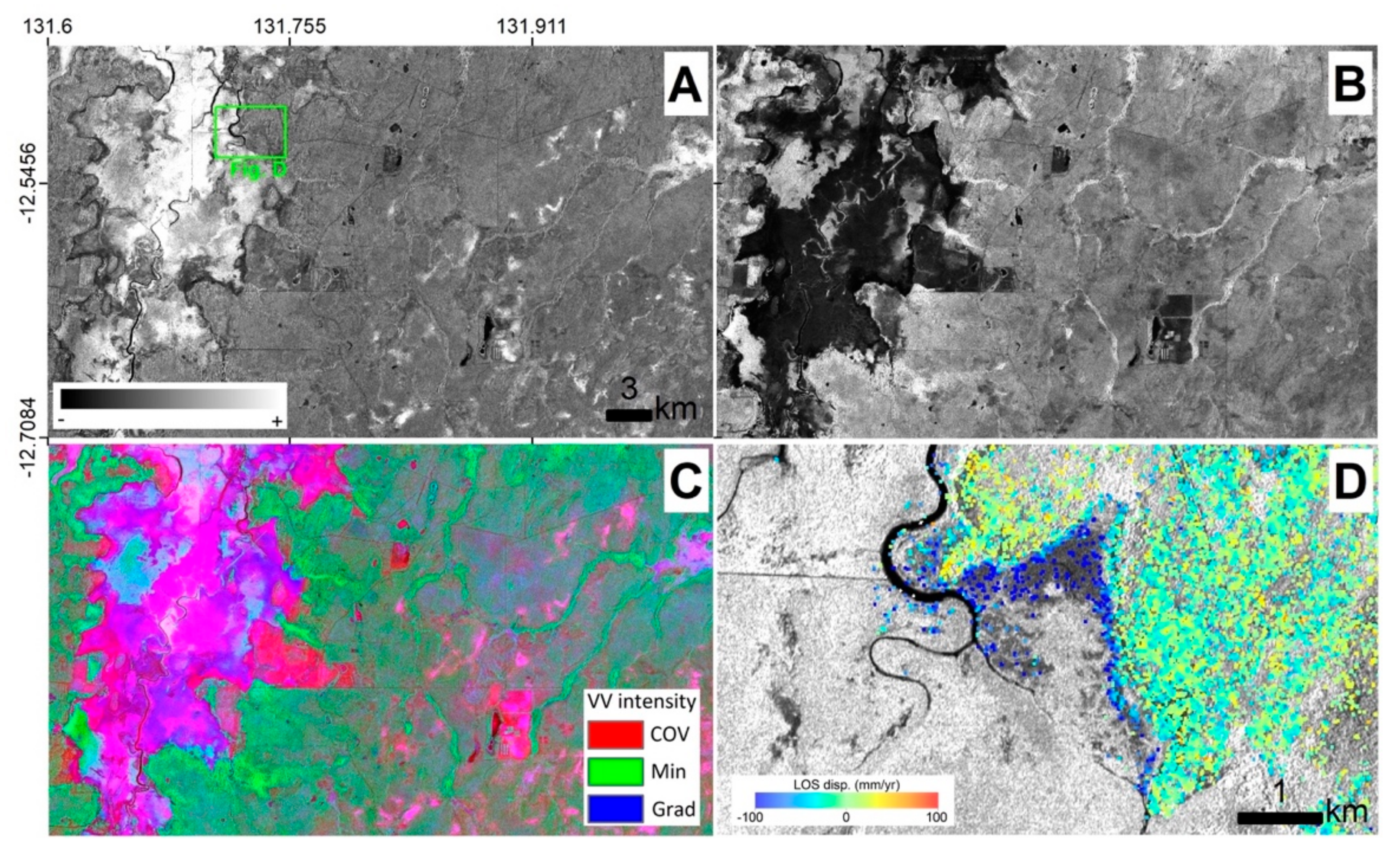
3.1.1. Example Case Study: Wildman Coastal Floodplains (Northern Territory)

The wetlands of the Wildman coastal floodplains, Northern Territory (for location, see Figure 2A), are an example where SAR provides a method of mapping inundation amongst and beneath vegetation. While a simple amplitude thresholding might be used as the first approach or for simple cases (Section 2), it is important to keep in mind that complex and/or mixed land covers (water, aquatic and semi-aquatic vegetation, and partly inundated forests) might challenge the interpretation of the SAR backscattering signal. The amplitude of the returned signal is impacted by plant density and physical structure, which modifies the partitioning between direct, volumetric, and double-bounce scattering. Open-water and low-aquatic vegetation is typically well-retrieved by such an amplitude thresholding approach, whereas inundated forests induce high values of SAR intensity due to a particular water-trunk double-bounce scattering (e.g., used in [23,24]). Therefore, a more complex scattering mechanism retrieval is required (e.g., see [27] for information on SAR-scattering mechanisms over wetlands).

In this example, flooding patterns and surface-water bodies are mapped using time-series analysis of 49 Sentinel-1 Interferometric Wide swath (IW) SAR backscatter intensity images (co-polarised vertical transmit, vertical receive (VV)) to extract the minimum and maximum, temporal gradients, and Coefficient of Variation (COV; the standard deviation divided by the mean) (Figure 3). Seasonally flooded areas are associated with high COV (red in Figure 3A), whereas flat and rapidly flooded areas are identified as having a high temporal gradient (maximum absolute variation between consecutive acquisition dates; blue in Figure 3A), and vegetated, flood-free areas have a high-temporal minimum with low-temporal variability (green in Figure 3A).

Advancing and receding seasonal flooding can be mapped between consecutive image acquisitions (12-day intervals for Sentinel-1) by identifying pixels with intensity below a threshold (−15 dB selected based upon histogram analysis). The floodplain dynamics (red on Figure 3) do not permit ligneous vegetation to grow, and hence no major influence of double-bounce scattering, increasing SAR intensity during flood events, is expected. An example for a precipitation event in February 2018 is shown in Figure 3B,C, respectively, with a time-series of the SAR-derived percentage of flooded areas throughout the observation period (from 20160805 to 20180409) shown in Figure 3D.

This example illustrates SAR’s potential for mapping the extent of floodwaters in vegetated areas, which is significant for coastal floodplains in Australia, where inundation impacts infrastructure development and the long-term evolution of sensitive ecosystems that are particularly susceptible to the impacts of sea-level rise (e.g., [24]). It also highlights the challenges of applying simple intensity thresholding in environments where multiple concomitant factors influence the strength of the returned signal. For example, terrestrial (or semi-aquatic) plant growth during dry seasons decreases the VV intensity returns over dry floodplains (Figure 3D—areas below −15dB increasing in proportion from July to October), whereas aquatic plant growth during flooding season (Figure 3D—January–April) might increase the VV intensity returns over flooded areas through double-bounce scattering. These factors should be considered when developing operational SAR map products for similar environments, as simple intensity thresholding may result in inaccuracies. To some extent, the use of multiple polarizations reinforces such analysis by protecting from potential false-positives, e.g., HV and VH bands being less sensitive to water surface waves and perturbations than HH and VV bands [28].

3.2. Drought and Unsustainable Groundwater Extraction

Much of Australia is characterized by low-precipitation rates in the range of 300–700 mm/yr [29]. Groundwater extracted from subsurface aquifers comprises a large percentage of the available water and ensuring that the balance between groundwater recharge and extraction is maintained is essential to sustain this resource. SAR imagery provides opportunities to assess multiple surface expressions of groundwater dynamics.

Firstly, information about the discharge and availability of shallow groundwater can be inferred by detecting and monitoring Groundwater Dependent Ecosystems (GDEs: [30]). GDEs are a frequent surface expression of groundwater across Australia, and any impact on groundwater resources will be seen in groundwater-dependant vegetation health (after a time delay that is dependent upon vegetation resilience and aquifer types). Vegetation health metrics are typically derived from multi-spectral EO sensors (e.g., Landsat: [31]), but recent assessments of Australian GDEs demonstrate that SAR imagery could overcome the limitations of multispectral-based approaches. SAR sensing offers temporally stable image time series (unaffected by the cloud cover) and, by taking advantage of radar signal penetration into the canopy, provides information on the vegetation leaf-branch structure (rather than its surface reflectance as is the case of multi-spectral images). By analysing the seasonal variations in time-series of Sentinel-1 SAR intensity and InSAR coherence, Ref. [32] showed that GDE monitoring is, for the first time, possible with SAR imagery on a yearly timescale. The SAR-based GDE mapping showed >90% similarity to the Global GDE Atlas [31], suggesting that SAR imagery could benefit future monitoring of groundwater-dependent vegetation.

Secondly, the ground displacement information from InSAR is used to characterize and evaluate groundwater management strategies around the World [18,33,34], including in Australia [35]. This is because variations in groundwater storage modify the hydraulic pressure in subsurface mixed-sedimentary aquifers and aquitards, leading to structural changes in compressible sediment layers (the theory of poroelasticity). A hydraulic-pressure decrease results in subsidence, with long-term (i.e., not a transient seasonal trend) subsidence indicative of inelastic (irrecoverable) aquifer compaction, which may result in the permanent loss of porosity within the aquifer and thus a decrease in its ability to store water (e.g., [18]). Conversely, aquifer recharge, including artificial managed aquifer recharge (MAR), causes hydraulic pressure to increase and may result in uplift, although observations of this phenomenon are scarce.

Monitoring and characterisation of such ground displacements are also necessary in order to mitigate subsequent damage to above- and below-ground infrastructure (including pipes, powerlines, buildings, and roads). For subsidence, ground displacement monitoring is necessary to assess potential impacts upon flood risks, as subsidence can act to amplify relative sea-level rise, risking tidal inundation of areas that were previously above the high-tide line and degrading coastlines. More than 80% of Australia’s population live within 50 km of the coast [29], and in low-lying coastal areas, accurate measurements of land subsidence linked to groundwater extraction are valuable for risk assessments of the effects of sea-level rise [36].

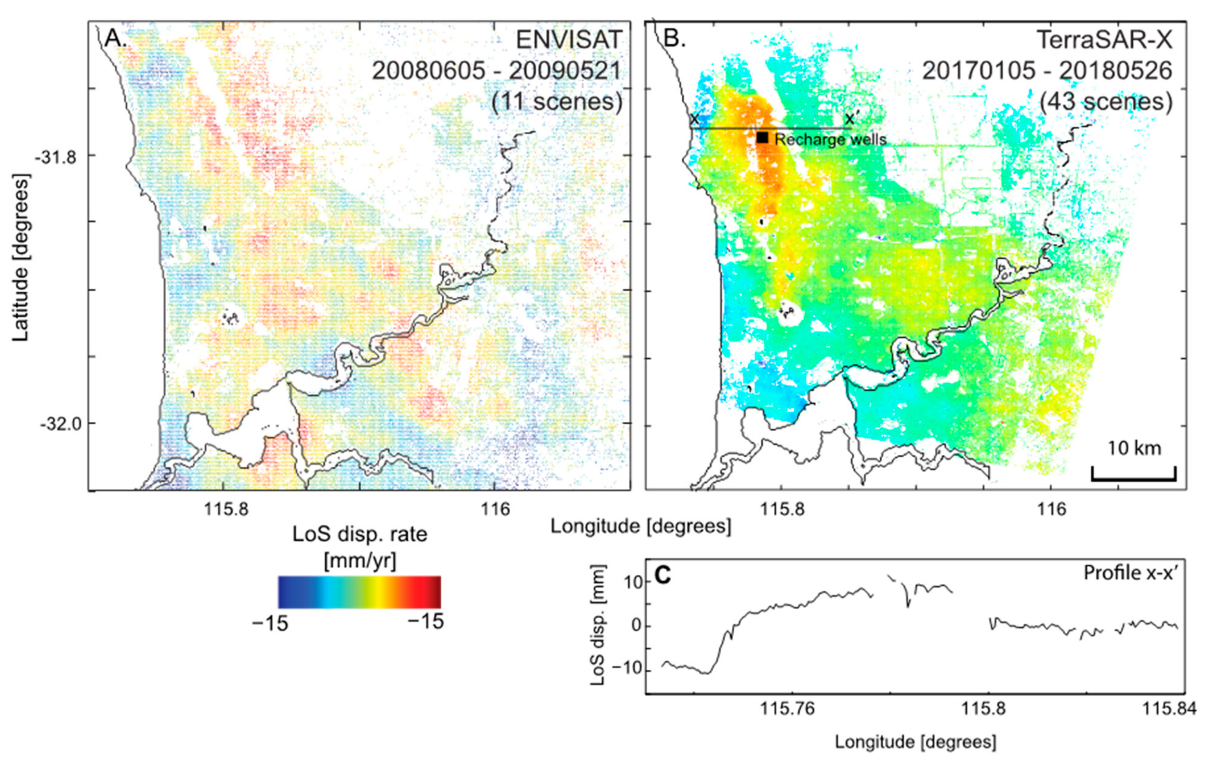
3.2.1. Example Case-Study: Groundwater Extraction and Recharge (Perth, Western Australia)

In Perth, Western Australia, rapid increases in the volume of extracted groundwater from subsurface aquifers between 2000 and 2005 is correlated with subsidence of up to ~7 mm/yr detected from continuous Global Navigation Satellite System (GNSS) measurements [37]. More recently, in August 2017, MAR activities commenced as part of the city’s long-term groundwater management strategy. Perth is, therefore, an example where assessments of both groundwater extraction and recharge could be supported by InSAR measurements of subsidence and uplift.

However, although SAR data have been acquired over Perth since the 1990s from ERS-1/2, ENVISAT ASAR, and ALOS PALSAR [38,39], short time-series (e.g., Figure 4A) and gaps in time-series (e.g., 12 scenes acquired over a 5-year period: [38]) make assessments of the time-history of displacements challenging. This includes the initial period of Sentinel-1 operations, during which imagery was acquired at 24-day intervals for a 9-month period between August 2015 and May 2016 [40]. The results of these datasets are saturated by atmospheric noise [39] or capture only seasonal displacements, which are shown from levelling to be cm-scale (e.g., [41]).

An assessment of a longer InSAR time-series is required to determine the recent rate of longer-term (multi-year) subsidence in Perth [40], which from levelling surveys is expected to be <10 mm/yr [37,41]. These data are now available from Sentinel-1, which has provided imagery at 12-day intervals since 2016.

In Perth, subsidence may now be counteracted by the impacts of MAR activities. Ground displacement observations made since the onset of MAR in August 2017 using TerraSAR-X suggest that, since recharge began, the hydraulic pressure in subsurface aquifers has increased enough to cause uplift proximal to the injection wells (Figure 4B). More than >10 mm of positive LoS displacement is observed between January 2017 and April 2018 (Figure 4B). Ongoing InSAR monitoring, combined with ground-based geodetic infrastructure [15], will be key to the characterisation of the impacts of MAR, including the effects upon long-term subsidence in this region.

The example of Perth demonstrates the past challenges in using InSAR data to aid Australian groundwater management strategies due to the variable temporal coverage of data. Applications in this setting are consequently limited, whereas InSAR has been applied extensively worldwide to quantify the impacts of groundwater extraction. Yet observations of local-scale effects in Perth and an example of large-scale (14,000 km²) monitoring in the Gippsland Basin, Victoria [42,43], highlight the potential for better integrating these measurements into groundwater management practices on both local and regional scales, which is now possible with consistent Sentinel-1 data time-series.

4. Fire Monitoring

Controlled and uncontrolled fires play a key role in Australian ecology (e.g., [44]) and present a significant hazard to life, impacting 100,000s km² each year. Operational usage of optical EO datasets available at multiple times each day (e.g., MODIS, VIIRS Suomi NPP, AVHRR, and Himawari-8) to produce fire hotspot detection point data (and in some instances, fire-affected area products) have aided fire management activities, with information available on web interfaces hosted by state and federal government (e.g., MyFireWatch myfirewatch.landgate.wa.gov.au and DEA Hotspots hotspots.dea.ga.gov.au—both accessed on 16 March 2021).

Whilst the potential contribution from current open-access SAR data to remote fire detection is limited by the temporal separation between satellite overpasses (days rather than hours or minutes), mapping of burned areas using SAR has been demonstrated in numerous locations using change-detection in backscatter imagery and InSAR coherence (e.g., Section 2; [44]). Compared to other EO sensors, SAR data is advantageous when fires are still active nearby as it is able to detect changes on the ground through smoke and ash that may inhibit other sensors. Due to the penetration of the SAR signal through vegetation, there is also scope to measure the burning of understorey vegetation not visible to optical sensors. Thus, interest lies in the use of these data to complement other EO data types (mentioned above) for longer-term fire management objectives such as estimates of fuel load and annual burned area mapping to evaluate fuel age and the efficiency of controlled burns [45]. For example, ALOS PALSAR and PALSAR-2 data have been shown to reduce the misclassification of the unburned forest by 9% for eucalypt and 3% for coniferous forests (2009 Kinglake fire, Victoria: [46]) and estimate the impacts of prescribed burning of eucalypt forests in Western Australia to within 79% [47]. Consequently, there is scope to further integrate SAR into fire management practises across Australia.

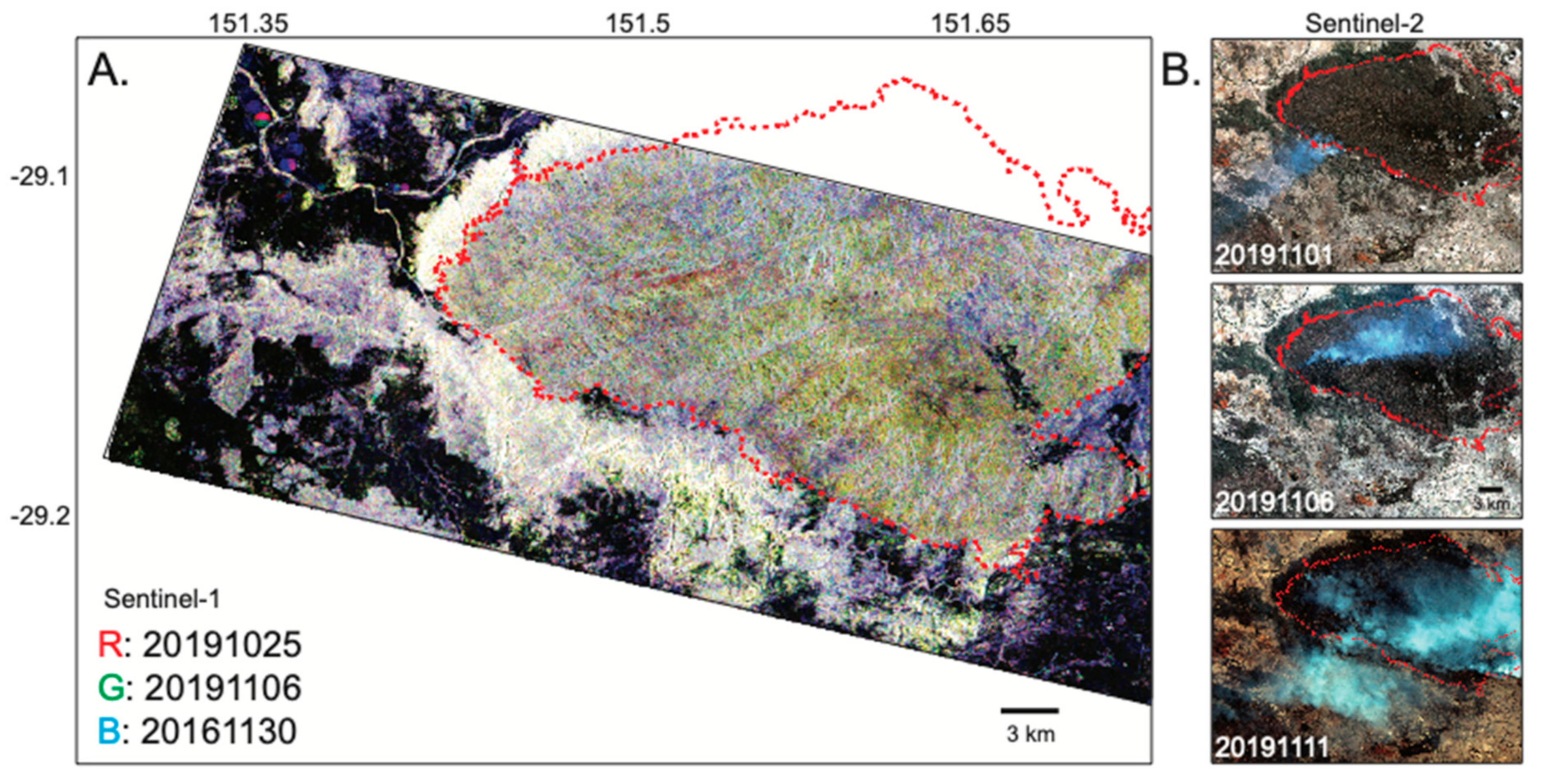
Example Case-Study: 2019 Torrington Fire (New South Wales)

Between November 2019 and January 2020, uncontrolled bushfires burned through more than three million hectares of New South Wales and Queensland. Activation of the International Charter Space and Major Disasters occurred on 13 November, and at the time of writing, 28 “wildfire situation” map products had subsequently been produced by Copernicus EMS using optical satellite datasets including Sentinel-2, SPOT6 and Landsat-8.

We assess the application of Sentinel-1 SAR to replicate such a map product by selecting a region covered by a Copernicus EMS burned area extent map derived from Landsat-8 imagery (map product 04TORRINGTON, v1 produced 20191113: [48]) in Torrington, close to the border of Queensland and New South Wales (see location in Figure 2A). A red-green-blue (RGB) change detection image was produced (Figure 5A) by assigning backscatter intensity images acquired prior to (20191025), during the onset of (20191106) and after (20191130) fires in this region to the red, green, and blue channels, respectively. The resulting RGB image (Figure 5A), is compared to the burned area extent obtained from Copernicus EMS (delineated by the red line), with Sentinel-2 imagery displayed for reference in Figure 5B.

From the composite SAR image, it is possible to infer some information about different burn stages. Red areas indicate backscatter that has decreased since 20191025 (potentially material burned between 20191025–20191106), and in this case, the red region at 151.5° E in Figure 5A corresponds to the location of burning at or before 20191106 visible in the Sentinel-2 image (Figure 5B middle).

There are a number of challenges in the interpretation of these data and in implementing operational tools based on SAR for fire mapping, particularly in the absence of ground-truth information. These include the dependency of the backscatter response upon the material burned (i.e., understory vegetation or tree canopy); moisture content; imaging geometry of the sensor; and the SAR wavelength (e.g., [44]), which dictates the depth of the signal’s penetration within the vegetation canopy and the sensitivity of the measurements to different sized scatterers (e.g., X-band—leaves; L-band—branches and trunks). Experiments with multiband SAR data (Section 7.1) will therefore strengthen the interpretation of these data, which require further testing to streamline the integration into operational burned area mapping [49].

5. Natural Resource Extraction

Australia’s prevalent below- and above-ground natural resource extraction industries (e.g., the largest global producer of iron ore, bauxite, rutile, and zircon: [29]) present subsidence and land-stability monitoring needs to reduce potential risks to people, infrastructure, equipment, and productivity (e.g., [50]). Consequently, ground-based geotechnical monitoring is routinely performed, but the measurements are restricted to localised areas (e.g., using slope-scanning radar) and/or sparsely distributed points (e.g., surveying), failing to cover the entire operation. Conversely, InSAR facilitates measurements of displacements over a whole extraction site, providing spatially and temporally dense constraints upon the extent and advancement of ground displacements, which can be applied to validate and improve predictive models of subsidence or slope instabilities (e.g., [51]).

Over the last 5–10 years, SAR and InSAR have begun to be incorporated into mine-site safety monitoring operations globally (e.g., [52]), facilitating complete monitoring of mine sites, including the stability of open pits walls/roads, waste piles [51], and tailings ponds and dams. The case studies presented in Section 5.1 and Section 5.2 are the result of projects undertaken to demonstrate the value of InSAR as a tool for monitoring mining operations. Section 5.3 then summarises the work that has been undertaken to assess the impacts of coal seam gas extraction in the Surat Basin. In addition to these examples, commercial providers deliver operational geotechnical monitoring products utilising SAR data at other resource extraction operations in Australia (e.g., [51]).

5.1. Below Ground Mining Operations

Underground longwall mining is the principal approach used in Australian coal mines operating at depths of >300 m, involving the total extraction of the panels of coal in corridors that are often several kilometres long by hundreds of metres wide. As the panel is progressively extracted, the roof is supported. When the support is removed, the overburden may collapse into the void. This downward movement of material can result in ground-surface subsidence of up to 1 metre directly above the extracted panel. The monitoring and management of this large magnitude subsidence are particularly critical where mines are located close to population centres (e.g., Tahmoor Colliery, NSW, located below the towns of Tahmoor and Thirlmere: Figure 6) and engineering structures (e.g., Tower Colliery, NSW, is overlain by a freeway that crosses a bridge over a river gorge).

Several studies have demonstrated the feasibility of using InSAR for monitoring subsidence at longwall coal mines in Australia (e.g., [4,53,54]). The evidence from the time-series analysis indicates that residual subsidence continues years to decades after mining activities cease (e.g., the Metropolitan Mine: [53]), emphasising the requirement for long-term ground displacement monitoring.

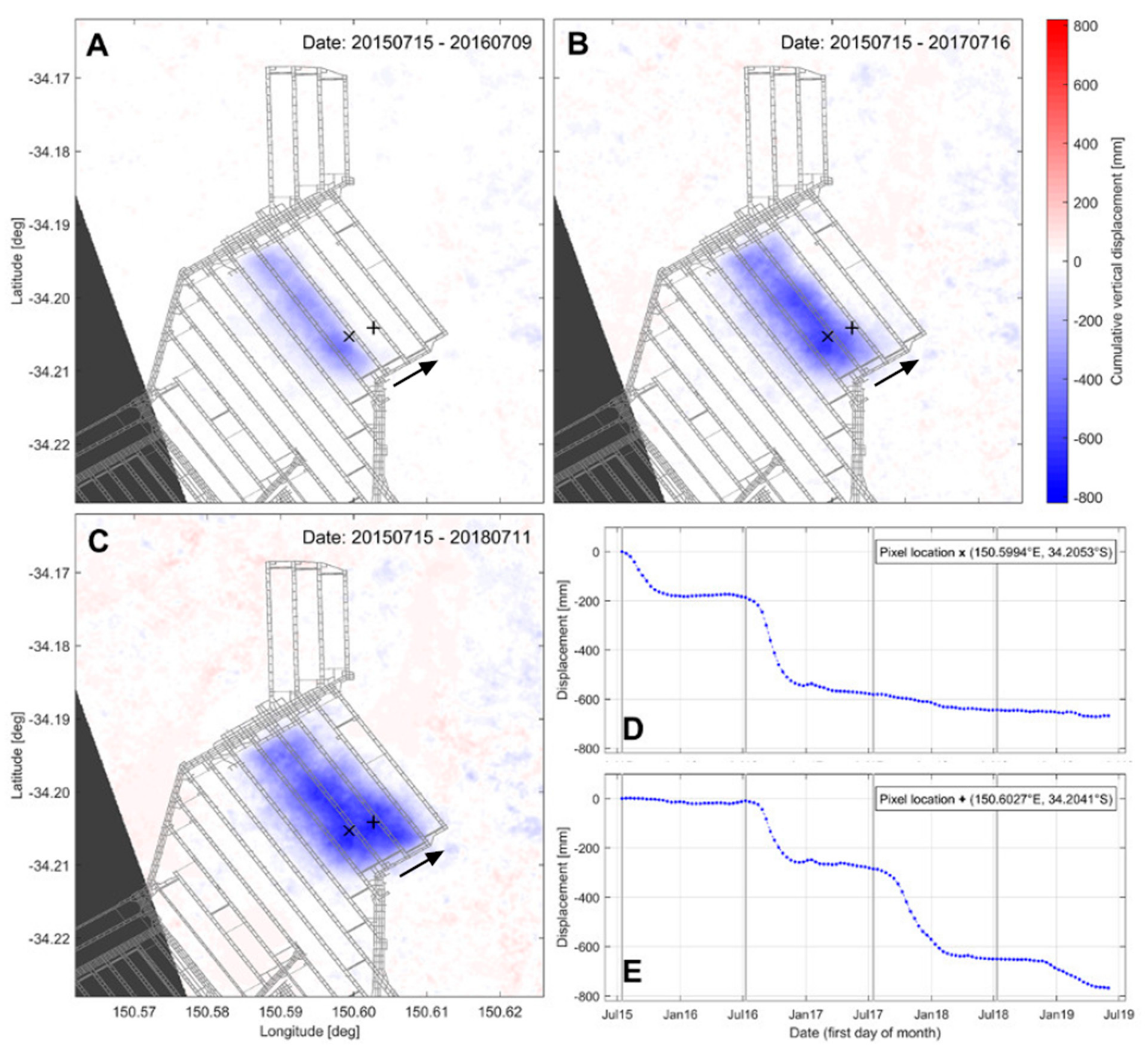
Example Case-Study: Tahmoor Longwall Coal Mine (New South Wales)

At the Tahmoor longwall coal mine, New South Wales (for location, see Figure 2A), we derive cumulative vertical displacements between July 2015 and May 2019 from InSAR analysis of ascending and descending orbit RADARSAT-2 data (Section 2). Maximum subsidence of −0.8 m is observed (Figure 6). Operations progress from one longwall to the adjacent longwall in the direction shown by the arrow in Figure 6A. Time-series of individual pixels can be used to track the time history of displacements at different stages of longwall operations and occurring due to interactions between adjacent longwall extractions (Figure 6D,E). The major subsidence shown in Figure 6D occurs in late 2015 and late 2016 and is mainly affected by the two adjacent longwalls. In contrast, the time-series shown in Figure 6E is not only affected by longwall operations in the adjacent longwalls (in late 2016 and late 2017/early 2018) but also by longwall operations further away from the pixel location (in late 2018/early 2019).

These observations are in qualitative agreement with ground-based measurements available in public reports [55]. However, unlike ground-based measurements, the InSAR analysis provides a dense spatial coverage of ground displacements for the full area capturing the spatio-temporal evolution of subsidence.

5.2. Above-Ground Mining Operations

Above-ground mining operations consist of open-pits (Section 5.2.1), waste piles, and tailings ponds and dams (Section 5.2.2). Accessible case studies of open-pit monitoring using SAR and InSAR within Australia are limited for commercial reasons, but for effective use of the information, mine site operators crucially require reliable, easy to interpret, and timely (within 24–48 h of acquisition) observations to effectively act upon potential risks [51].

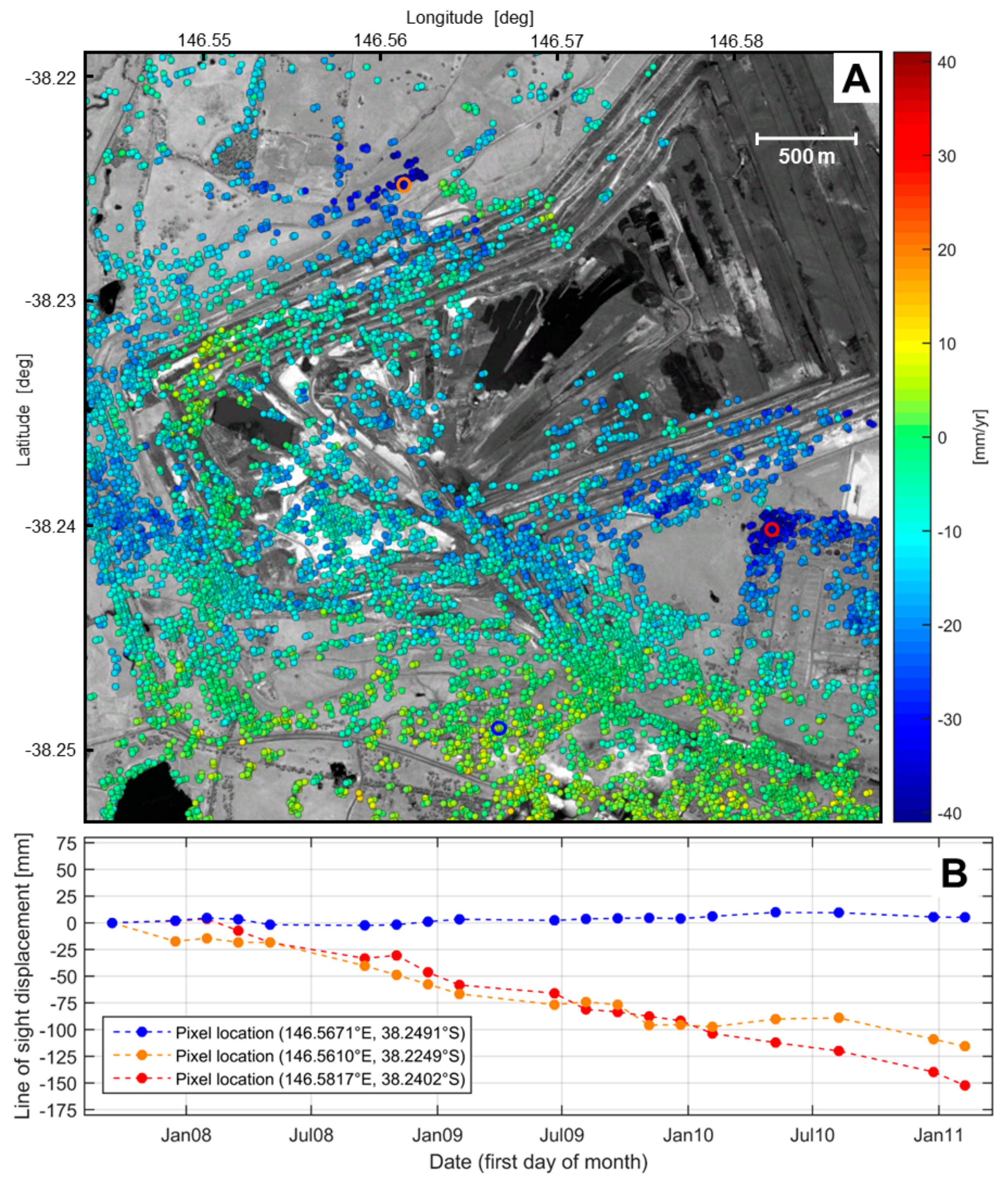
5.2.1. Example Case-Study: Latrobe Valley Open-Cut Coal Mines (Victoria)

In the Latrobe Valley, Victoria (for location, see Figure 2A), InSAR has been used to measure ground displacements at the Hazelwood and Loy Yang open-cut coal mines. At the Hazelwood mine, InSAR analysis by [43] revealed subsidence rates of >−60 mm/yr attributed to mining activities and associated groundwater extraction related to mine dewatering. Following a precipitation event, cracks were observed within the mine and nearby roads, resulting in the 7-month closure of a nearby major road. InSAR observations showed that this freeway had undergone a tilt of >0.5 mm/m [43].

At the Loy Yang mine, we use ALOS PALSAR data acquired between 2007–2011 to map LoS velocities (Figure 7A). At the edges of the mine, LoS velocities of up to −40 mm/yr are observed (Figure 7A), the majority of these displacements occurring at a constant rate within the analysed time period (see example time-series in Figure 7B). However, the coverage of coherent InSAR pixels directly coincident with the open-cut operations is limited by coherence loss over time as a result of rapid and regular changes of the surface (Section 2 Figure 7).

Other challenges in applying InSAR data to monitor the stability of open-pit mines include shadowing resulting from steep slopes (e.g., the lack of coherent pixels on the west-facing slope of Loy Yang mine in Figure 7A) and rapid or large magnitude displacements resulting in incoherence (as described in Section 2). To overcome this, both SAR backscatter offset tracking and interferometry can be applied to capture large magnitude (10–100s cm) and small magnitude (sub-cm) scale displacements, respectively. Coupled with SAR backscatter change detection to monitor surface changes (such as shifting-waste piles) from a single dataset, it is possible to capture the full extent of the deformation field across a mine site and identify potential hazards in areas with no other monitoring infrastructure.

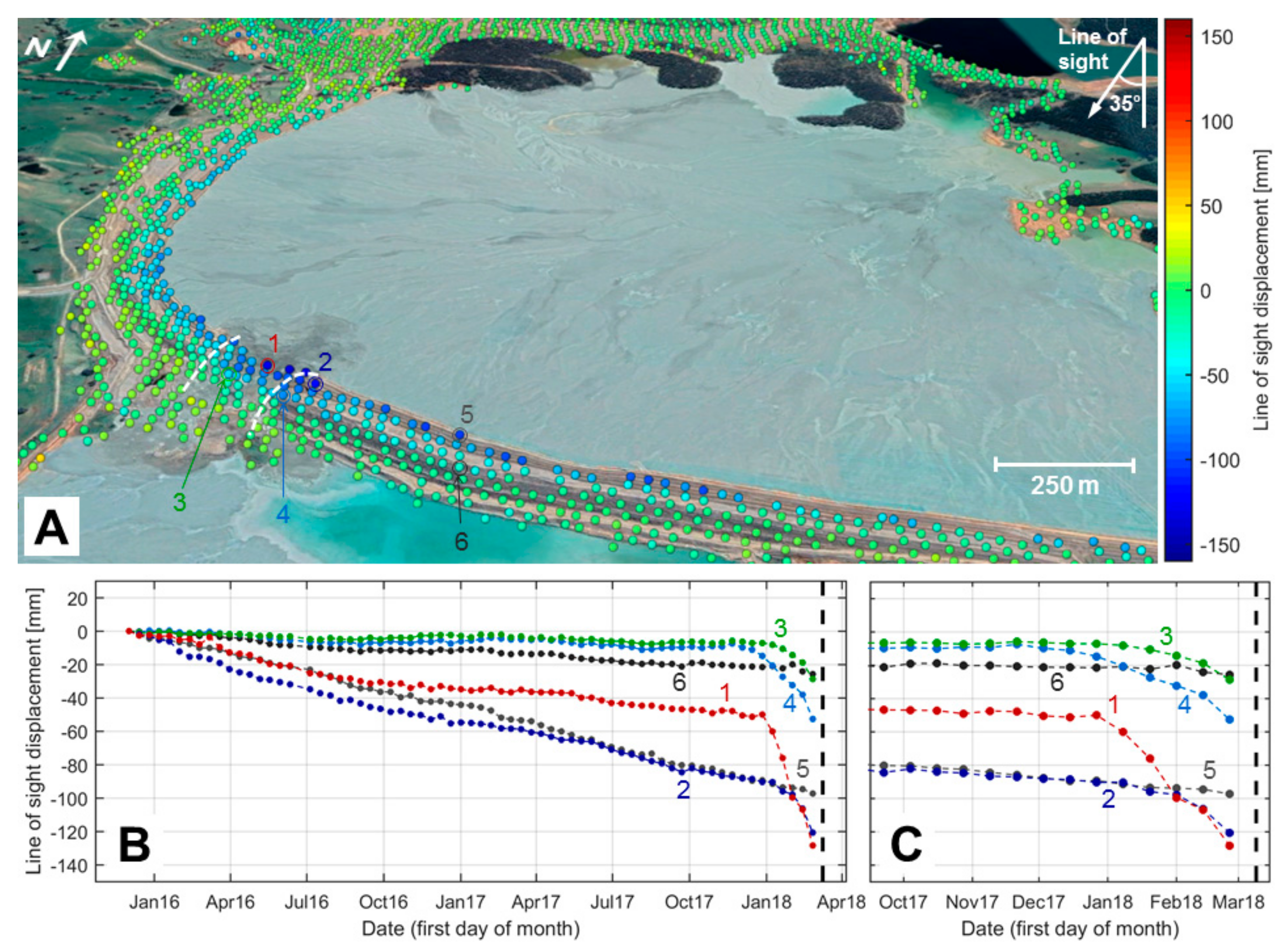
5.2.2. Example Case-Study: Cadia Tailing Dam Failure (New South Wales)

Solid and liquid tailings containment infrastructure within mine site operations can also be monitored using InSAR (e.g., [56]). In March 2018, partial failure of a dam wall occurred at a tailings storage facility at the Cadia gold mine, New South Wales, and the subsequent time-series analysis of Sentinel-1 imagery in the ~2 year period prior to failure reveals the potential for InSAR to provide early warning of collapse (Figure 8).

At the upper layers of the dam, steady motion totalling ~50 mm is detected over the 2-year observation period prior to collapse and is likely related to the expected settlement of new layers recently added to the earthen dam wall (points 1, 2, and 5; Figure 8). However, during the three months prior to collapse between late January to late February 2018, ~80 mm of motion is detected in pixels coincident with the zone of failure (points 1–4 in Figure 8B, where the white lines show approximate failure zone). Our identification of precursory motion is corroborated by other independent assessments of this event (e.g., [56]).

In addition to detecting the timing of significant changes, these measurements suggest that there is scope to use InSAR to identify the location of weaker or weakening parts of mine infrastructure since the magnitude of displacements is greater for InSAR pixels located within the part of the dam wall that later failed (points 1–4; Figure 8) than those located adjacent to it (points 5 and 6; Figure 8). Thus, InSAR could have potentially been used not only as an early-warning tool with a lead-time exceeding 1 month but also to map the weak area prior to failure and focus adequate mitigation efforts at these locations.

5.3. Coal Seam Gas Extraction

Other applications of SAR to monitor natural resource extraction in Australia include Coal Seam Gas (CSG) operations in the Surat Basin, southern Queensland. CSG extraction involves the removal of significant volumes of groundwater to depressurise the reservoir and allow gas to be released from the pore spaces in the host formation. Therefore, subsidence is a highlighted concern, and the use of InSAR has been recommended to aid in subsidence monitoring and development of a surface deformation prediction [57].

Baseline subsidence monitoring efforts in the Surat Basin using ALOS PALSAR imagery between 2006 and 2011 have revealed conflicting results. [58] did not identify any large-scale pattern of ground displacement with a magnitude greater than 8 mm/yr, whereas [59] identified displacements coincident with CSG mining at rates of up to −28 mm/yr. Consequently, this region is now the site of a network of 40 radar corner reflectors to validate relative ground displacements recorded by InSAR (from Sentinel-1 data on both ascending and descending passes) with ground-based absolute displacement measurements made with GNSS [60]. This will aid in further monitoring of this gas field.

6. Seismic Hazard Monitoring

Seismic activity may result in displacements of the Earth’s surface—a phenomenon that has been measured using InSAR since the 1990s [19]. Although Australia is situated in an intraplate setting, levels of seismicity are high when compared to areas of stable continental crust globally [61,62]. Large earthquakes do occur [63,64], including seven Mw 6.0 or above events since 1968, and there is potential for large intraplate earthquakes anywhere in the country [63,65]. Intraplate seismicity within Australia is noted to be shallow (e.g., [63]), and therefore, it is more likely to cause ground surface deformation and/or surface rupture (e.g., [66,67]).

The types and magnitudes of events that InSAR may be sensitive to in Australian conditions have been investigated, but InSAR has not routinely been used in response to seismic events in Australia, principally because of the lack of recent pre-earthquake images in the archive [66,68]. The coherence of interferograms decreases as the time separation between image pairs increases; therefore, without recent pre-earthquake imagery, it may not be possible to make a coherent InSAR measurement.

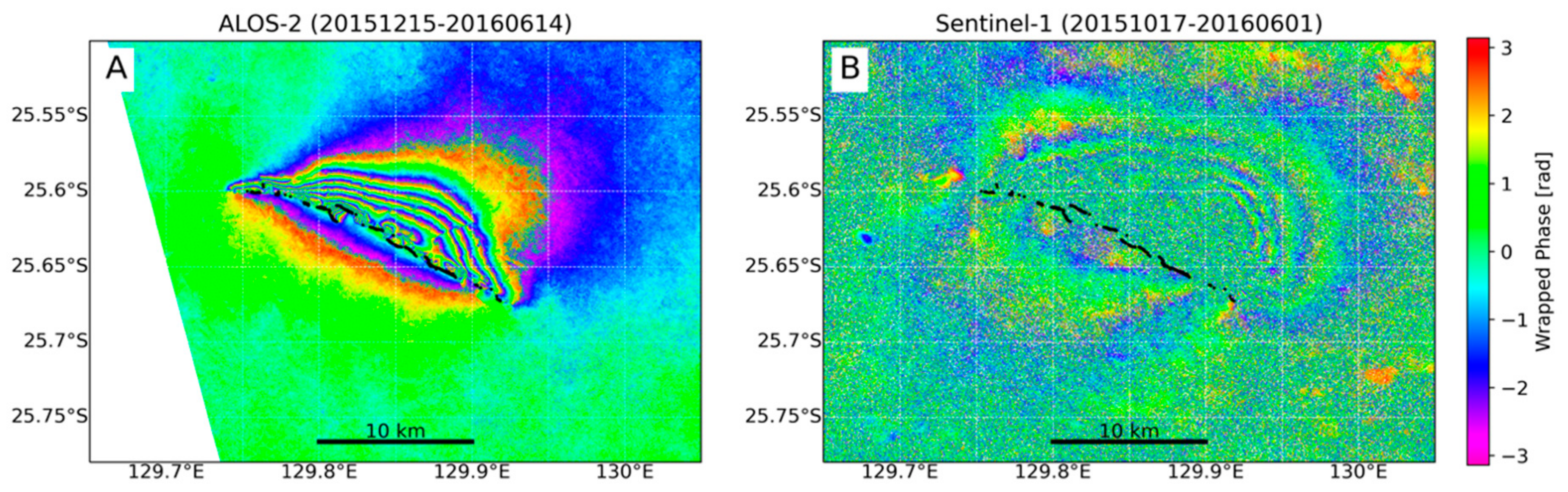
Example Case-Study: 2016 Mw 6.0 Petermann Ranges Earthquake (Northern Territory)

Access to pre- and post-earthquake imagery from Sentinel-1 and ALOS-2 facilitated observations of the 2016 Mw 6.0 earthquake in the Petermann Ranges, Northern Territory (for location, see Figure 2A). In this case, we formed co-seismic interferograms using post-earthquake SAR images that were acquired by ALOS-2 and Sentinel-1 (see Table S2 for sensor details) only upon request to the satellite operators (Figure 9). For both ALOS-2 and Sentinel-1, the time separation between the pre- and post-earthquake images was significant (182 and 228 days, respectively).

Due to the longer wavelength of the sensor (L-band: λ = 22.9 cm), the ALOS-2 co-seismic interferogram (Figure 9A) still has excellent coherence and was particularly useful in the period after the earthquake to remotely map the complex surface rupture pattern and enable field teams to focus mapping efforts on the ground [64]. In contrast, the co-seismic interferogram from Sentinel-1 (C-band: λ = 5.6 cm) is heavily de-correlated (Figure 9B), with coherence also lost due to the large magnitude of near-field displacements close to the surface rupture trace (the black line in Figure 9). At the time of the earthquake, Sentinel-1 had not yet commenced a regular acquisition strategy over the region. The now regular acquisition interval of Sentinel-1 is a game-changer in this regard and will enable more Australian earthquakes to be detected and analysed with InSAR in the future. This includes international efforts for the automated delivery of co-seismic InSAR map products. Whilst this has previously been limited to large magnitude events (e.g., NASA Jet Propulsion Lab’s Advanced Rapid Imaging and Analysis (ARIA: [69]), the LiCSAR platform [70] delivers interferometric products for all events above Mw 5.5 identified in the United States Geological Survey Comprehensive Earthquake Catalog. The results will complement Australian seismic monitoring, which currently relies upon a sparse sensor network (typical station spacing of >1000 km), by providing additional constraints upon epicentre location and source parameters for events that result in surface displacements.

7. Geomorphological Changes

Changes in the morphology (i.e., landforms and topography) of the Earth’s surface impact existing and future infrastructure. Sudden events (landslides, sinkholes, and cliff collapse) and progressive processes (erosion) pose hazards in both coastal and inland Australia (e.g., [71]) and may arise as the secondary effect of other hazards, such as flooding or fires (e.g., [72]). There is scope to use InSAR to measure changes in the height of Earth’s surface arising from these processes as a tool for monitoring geomorphological changes. The application of InSAR data to landslides and sink holes is well-documented by case studies in the literature (e.g., [17]), but for erosion and sediment transport, examples are more limited [73,74].

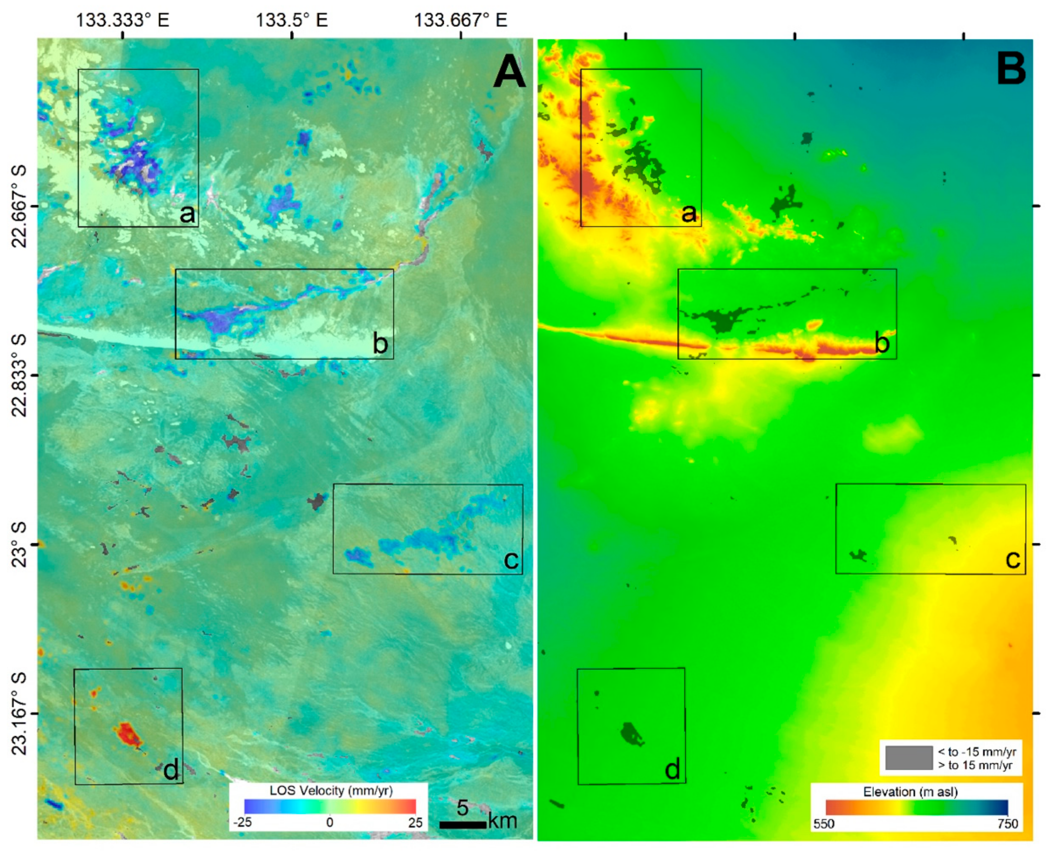
7.1. Example Case-Study: Geomorphological Monitoring in Remote Areas (Northern Territory)

To demonstrate this application in an Australian environment, we select two areas (see Figure 2A for locations) that experience significantly different levels of precipitation, using SAR and InSAR to map geomorphological changes linked to precipitation. The first location (Figure 10) experiences an annual rainfall of 1700 mm (see Figure 3 for applications of SAR to monitor flooding in this region), and the second (Figure 11) is located in a desert environment, experiencing an annual rainfall of 300 mm [29].

In the region of high precipitation, we initially use the method described in Section 3.1.1 and Sentinel-1 backscatter intensity imagery acquired over a one-year period between 20170108 and 20171222 to delineate the floodplain extent. Open flood plains are identified by high-intensity values in Figure 10A and high COV in Figure 10C, whereas sparse forest is identifiable throughout Figure 10A and B by the texture created by contrasting canopy/ground SAR responses, with increased COV (see Section 3.1.1; red in Figure 10C) in regions where the penetration of the SAR signal beneath the canopy allows the detection of temporary floodwaters.

In Figure 10D, InSAR is used to measure relative differential LoS velocities across the floodplain banks. Negative LoS velocity is observed on the floodplain banks relative to the (assumed stable) surrounding sparsely vegetated forest. This signal may be attributed to the ablation of fine-grained sediments from the floodplain banks such that small baseline interferometric coherence is not lost (e.g., [74]), but the resulting change in land surface height is measurable. Alternatively, a conceivable explanation for the signal is the shrinking of surficial sediments as they dry or that the observed phase signal is directly related to the soil moisture change and not surface displacement (e.g., [75]). Moreover, we note the importance of accounting for the noise/coverage trade-off related to incorporating intermittently coherent pixels (occurring over vegetated areas and other temporally dynamic land covers) into the phase-to-displacement inversion procedure [35,76,77].

The contrasting, near-desert environment shown in Figure 11 experiences precipitation events from November to April, when fine-grained surficial sediments are prone to mobilization at rates dependent upon precipitation, slopes, and soil permeability/roughness.

As in Figure 10D, InSAR measurements using images acquired between 20170504 to 20190314 were used to identify regions of relative surface velocities that may provide insight into sediment transport and/or swelling/shrinkage due to changes in water content (e.g., [35,74]). Positive LoS displacements are identified corresponding to temporary ponds or salt lakes in flat areas (e.g., area labelled d in Figure 11), and negative LoS velocities are observed proximal to topographic gradients (e.g., areas labelled a, b, c in Figure 11).

In both of these locations, InSAR provides high-resolution measurements of surface changes, the characterisation of which provides key inputs into future plans for safe infrastructure development. However, satellite SAR observations require validation with field-based measurements to verify the cause of the observed signals and determine whether they result from weathering, sediment ablation/deposition, or shrinking/swelling in response to hydrological changes. Consequently, whilst there is promise for InSAR data to contribute to the study of geomorphological hazards, more validation is required to fully understand the link between the observed signals and geomorphological processes.

8. Discussion: Future Opportunities for Developing the Role of SAR for Hazard Monitoring in Australia

Over the last decade, a persistent message from the government and industry has been that SAR data are too expensive to be an economically viable tool for hazard (and other) monitoring and investigation, particularly over regional scales (e.g., [35,38]). As is the case for other countries globally, Australia’s capacity to use SAR data for hazard monitoring applications will therefore be largely dependent upon the availability of open-access data from existing and new sensors. Significantly, Sentinel-1 is the first satellite constellation to change the paradigm of the past years, providing wall-to-wall continental-scale coverage of open-access SAR data in Australia at regular repeat intervals. As is demonstrated in case studies here, this can be bolstered by access to additional commercial datasets, for example, at a higher spatial resolution, from pay-to-use satellite missions, which are now utilising smaller, lower-cost satellite platforms to reduce the cost of SAR data (e.g., ICEYE: Table S2).

In addition to data availability, progress towards the operational use of SAR in hazard monitoring by national and state government agencies in Australia (and elsewhere) will benefit from a number of other factors. The first of these is data access: downloading Sentinel-1 datasets from European/North American-based datacentres is problematic in the Asia-Pacific region, and therefore, a local data access node, the Sentinel Australia Regional Access (SARA) hub (https://copernicus.nci.org.au/sara.client/#/home—accessed on 16 March 2021), has been implemented to mirror all Sentinel-1 data acquired over the Asia-Pacific region and significantly expedite local data download times.

Standardised data formats or ‘Analysis Ready Data’ (ARD) products (for example as defined for SAR by the Committee on Earth Observation Satellites ARD for Land, CARD4L, initiative: [78]), standardised data platforms, and standardised analysis tools built upon open-access software (e.g., the SAR DataCube: [10]) will also support increased uptake of SAR data. Accordingly, plans for the inclusion of Sentinel-1 SAR data within DEA are underway and will further enable users to take advantage of this systematically acquired and openly available resource. Other resources include automated generation of InSAR products, e.g., seismic events, as described in Section 6. Crucially, the planned follow-on Sentinel-1 satellites (Sentinel-1C and D), plus Sentinel-1 Next Generation, will promote the longevity of any operational analysis tools developed for these data.

The consistent and systematic data provided by Sentinel-1 presents opportunities to implement SAR as a systematic tool (either operational or experimental) for monitoring and understanding the hazards described in this study. This will be key to developing, for example, a more comprehensive understanding of fault systems and seismic hazards, which is required for nation-building infrastructure projects and expansion of population centres (e.g., [79]). SAR-derived measurements are also now beginning to contribute to compliance in Australian infrastructure projects, such as tunnelling and resource extraction, including the mining and groundwater sectors (e.g., [7]). For example, it has been recommended that the regional InSAR survey of the Gippsland Basin, Victoria, (Section 3.2.1) be repeated every 3–5 years [80]. Mining operations are required to assess potential subsidence impacts as part of Environmental Impact Statements, and the ongoing validation and updating of subsidence predictions are set to benefit from a monitoring system that can fully capture the spatio-temporal extent of subsidence, such as is the case with InSAR (Section 5).

In light of the increased use of InSAR as a geodetic tool to monitor anthropogenic activities, networks of artificial corner reflectors have been installed to act as persistent high-amplitude reflections in SAR imagery and ties to Australia’s growing ground-based GNSS infrastructure (e.g., Surat Basin: [60]; Perth: [15]; southwest Sydney: [81]). Combining InSAR with absolute geodetic techniques acts to validate the measurements and enable the integration of relative InSAR displacement maps into absolute reference frames defined by the GNSS sites (e.g., [82]), with proposed extensions of this approach to the Australian (and global) network of Very Long Baseline Interferometry telescopes [83].

8.1. Synergies between SAR and other EO Data Types for Hazard Monitoring

In addition to increases in the volume of available SAR data, the growing volume and variety of available EO datasets lends itself to identifying new ways to exploit synergies between multiple sources of EO data to improve the spatial resolution of measurements, extend observation time-series, increase signal to noise ratios, and improve the interpretation and/or usability of final data products. For SAR-based hazard monitoring in Australia, three data synergies are identified to be of particular promise, including the integration of SAR with Gravity Recovery and Climate Experiment (GRACE) missions measurements of time-variable gravity, multi-spectral EO imagery, plus the integration of SAR data acquired across multiple frequency bands.

GRACE and the follow-on GRACE-FO monitor temporal changes of Earth’s gravity field that, on the time-scale of the observations (2002–2017 and 2018–present, respectively), are largely dominated by the effects of water storage change. Given the water management challenges that face many countries globally, GRACE and GRACE-FO data provide a valuable source of remote large-scale observations, but at a resolution (250–400 km) that is too low to be directly applicable to many water management activities [34]. Downscaling strategies often utilise auxiliary higher-resolution observations of mass change (e.g., [34]), which are relatively easy to obtain for surficial mass changes (e.g., glacial mass losses: [84]) but challenging to obtain for sub-surface masses such as groundwater. In this instance, large-scale InSAR-derived ground displacement maps (Section 3.2.1) can be used as a proxy for groundwater mass change distribution, offering an unprecedented opportunity to fill this gap [34,35]. It is important to note, however, that any non-groundwater mass changes, such as soil moisture storage change, surface water storage change (e.g., [34,84]), or mine extraction (as shown in the Northwest of Australia [85]), have to be subtracted to GRACE total mass change data to extract the groundwater storage change map used in the downscaling procedure.

Floods, erosion, landslides, fires, and groundwater depletion can be exacerbated by anthropogenic perturbations of the land cover such as logging, grazing and vegetation clearance (e.g., [86]). Multi-spectral EO imagery is used for land-use/cover classification (LUCC), but SAR provides a complementary dataset for this purpose, providing information about the physical structure of features on the ground (angle, orientation, roughness, and texture) to reduce ambiguities in these statistical classifications (e.g., [87,88]). While numerous other studies have explored such synergies for LUCC, no published studies from Australia are available to date.

Similar to how SAR and multi-spectral imaging provide information about different physical properties of features on the ground, SAR sensors operating at different frequencies (e.g., Table S2) provide different information due to the role of the SAR wavelength in influencing interactions of the microwave with scatterers of different sizes, the scattering mechanism (direct, double-bounce, volumetric: Section 2) and the penetration of the radar signal into the volume of ground targets. Different SAR frequency bands can be integrated for improving, e.g., LUCC classification accuracy (e.g., [24,89]), and there is currently scope to test a larger SAR frequency range than ever before with imagery now available at C-band (Sentinel-1), X-band (commercial providers), L-band (commercial providers but with future open-access from the NISAR mission due for launch in 2021, plus other missions such as ESA’s ROSE-L in due course) and S-band (NovaSAR-1).

8.2. Opportunities for Near-Real-Time Applications with New SAR Satellites

What is most noticeably lacking from the case studies presented here are examples of SAR being used for near-real-time hazard response. During unfolding disasters that demand an emergency response, immediate access to EO data is required if it is to be used to build situational awareness, aid in the effective deployment of resources, and inform damage assessments within a useful time frame. The benefit of using SAR in these instances is its ability to operate day and night, in all weathers, with radar capable of penetrating cloud, fog, rainfall, aerosols, and smoke. However, the time of image acquisition and subsequent latency between image acquisition, delivery, and processing, have been major limitations to applications of these data in response to rapidly advancing hazards, such as flash floods and uncontrolled fires (e.g., [7,22]). Some improvements have been found in the use of commercial data (e.g., by the Western Australia state geodetic agency during cyclone Bianca, 2011, in Western Australia 2011 [90]), but this has been found to be cost-prohibitive [22] unless the International Charter Space and Major Disasters is initiated. A new generation of commercial SAR sensors may offer improvements with lower image costs and sub-hourly orbital repeat (e.g., ICEYE: see Table S2 for details).

For Australia, the availability of SAR data for hazard response closer to near-real-time will be boosted by the country’s first activities in the direct tasking and operation of a civilian EO satellite as part of the NovaSAR-1 mission [8]. This satellite is expected to provide expedited observations over Australia, with data downlinked directly in-country for processing and distribution in closer to near-real-time than has previously been possible [91]. This will improve hazard response efforts through the use of SAR backscatter for damage identification, monitoring and assessment after fires, cyclones, floods, and earthquakes [8,9,91].

9. Conclusions

Effective disaster risk reduction benefits from comprehensive hazard monitoring. Satellite SAR imagery provides particular advantages for identifying and assessing hazards compared to other types of EO data, most notably due to its ability to see through cloud, smoke and, to a varying degree, vegetation; to measure displacements of the Earth’s surface; to “see” structural changes that are not related to surface reflectance and are not visible with optical datasets. The availability of systematically acquired SAR data by Sentinel-1 presents new opportunities to use SAR and InSAR to address national-scale hazard monitoring requirements, including for countries such as Australia, where uptake of these data has historically been limited.

New case studies that apply SAR data to issues critical to Australia and elsewhere, such as groundwater management, fires, resource extraction industries, and seismic hazard, highlight the potential contribution of these data to hazard monitoring efforts but also the potential challenges involved in the integration of SAR into operational systems. The case studies expand on the types of hazards previously investigated using SAR globally and provide an understanding of past, current, and potential future usage of these data for hazard monitoring applications in an Australian context, with insights that can be learned by the global community. The uptake of SAR data for hazard applications globally will continue to benefit from validated case studies, the development of tools (such as Analysis Ready Data and Open Data Cubes) that support operational use and, ultimately, the continued provision of open-access, consistent imagery by large-scale satellite missions.

References

1. United Nations Office for Disaster Risk Reduction. Available online: https://www.unisdr.org/we/inform/terminology#letter-h (accessed on 15 July 2020).
2. Held, A.; Clayfield, K.; Ward, S.; Dyke, G.; Harrison, B. Continuity of Earth Observation Data for Australia: Research and Development Dependencies to 2020; CSIRO Astronomy and Space Science: Canberra, Australia, 2012. [CrossRef]
3. Australian Earth Observation Community Plan 2016: Delivering Essential Information and Services for Australia’s Future. Available online: https://www.eoa.org.au/aeocp-the-plan/ (accessed on 15 July 2020).
4. Dhu, T.; Dunn, B.; Lewis, B.; Lymburner, L.; Mueller, N.; Telfer, E.; Lewis, A.; McIntyre, A.; Minchin, S.; Phillips, C. Digital earth Australia–unlocking new value from earth observation data. Big Earth Data 2017, 1, 64–74. [Google Scholar] [CrossRef] [Green Version]
5. Adam, N.; Kampes, B.; Eineder, M. Development of a scientific permanent scatterer system: Modifications for mixed ERS/ENVISAT time series. In Proceedings of the Envisat & ERS Symposium 2005, Salzburg, Austria, 6–10 September 2004; Volume 572. [Google Scholar]
6. Mueller, N.; Lewis, A.; Roberts, D.; Ring, S.; Melrose, R.; Sixsmith, J.; Lymburner, L.; McIntyre, A.; Tan, P.; Curnow, S.; et al. Water observations from space: Mapping surface water from 25 years of Landsat imagery across Australia. Remote Sens. Environ. 2016, 174, 341–352. [Google Scholar] [CrossRef] [Green Version]
7. Milne, A.K.; Williams, M.; Mitchell, A.; Watt, M. SAR Application Case Studies, Robust Imaging from Space, Adjunct Reference Document #2, CRCSI Report. Available online: https://www.crcsi.com.au/assets/Uploads/Files/Adjunct-Reference-2-SAR-Application-Case-Studies-FINAL.pdf (accessed on 15 July 2020).
8. Bird, R.; Whittaker, P.; Stern, B.; Angli, N.; Cohen, M.; Guida, R. NovaSAR-S: A low cost approach to SAR applications. In Synthetic Aperture Radar (APSAR) 2013 IEEE Asia-Pacific Conference; IEEE: Piscataway, NJ, USA, 2003; pp. 84–87. [Google Scholar]
9. Held, A.; Zhou, Z.S.; Ticehurst, C.; Rosenqvist, A.; Parker, A.; Brindle, L. Advancing Australia’s Imaging Radar Capability Under the Novasar-1 Partnership. In IGARSS 2019–2019 IEEE International Geoscience and Remote Sensing Symposium; IEEE: Piscataway, NJ, USA, 2019; pp. 8370–8373. [Google Scholar]
10. Ticehurst, C.; Zhou, Z.S.; Lehmann, E.; Yuan, F.; Thankappan, M.; Rosenqvist, A.; Lewis, B.; Paget, M. Building a SAR-Enabled Data Cube Capability in Australia Using SAR Analysis Ready Data. Data 2019, 4, 100. [Google Scholar] [CrossRef] [Green Version]
11. Lu, Z.; Zhang, J.; Zhang, Y.; Dzurisin, D. Monitoring and characterizing natural hazards with satellite InSAR imagery. Ann. GIS 2010, 16, 55–66. [Google Scholar] [CrossRef]
12. Flores-Anderson, A.I.; Herndon, K.E.; Thapa, R.B.; Cherrington, E. The SAR Handbook: Comprehensive Methodologies for Forest Monitoring and Biomass Estimation; SERVIR Global Science Coordination Office: Huntsville, AL, USA, 2019. [Google Scholar] [CrossRef]
13. Freeman, A.; Durden, S.L. A three-component scattering model for polarimetric SAR data. IEEE Trans. Geosci. Remote Sens. 1998, 36, 963–973. [Google Scholar] [CrossRef] [Green Version]
14. Bürgmann, R.; Rosen, P.A.; Fielding, E.J. Synthetic aperture radar interferometry to measure Earth’s surface topography and its deformation. Annu. Rev. Earth Planet. Sci. 2000, 28, 169–209. [Google Scholar] [CrossRef]
15. Parker, A.L.; Featherstone, W.E.; Penna, N.T.; Filmer, M.S.; Garthwaite, M.C. Practical Considerations before Installing Ground-Based Geodetic Infrastructure for Integrated InSAR and cGNSS Monitoring of Vertical Land Motion. Sensors 2017, 17, 1753. [Google Scholar] [CrossRef] [Green Version]
16. Wright, T.J.; Parsons, B.E.; Lu, Z. Toward mapping surface deformation in three dimensions using InSAR. Geophys. Res. Lett. 2004, 31, L01607. [Google Scholar] [CrossRef] [Green Version]
17. Intrieri, E.; Raspini, F.; Fumagalli, A.; Lu, P.; Del Conte, S.; Farina, P.; Allievi, J.; Ferretti, A.; Casagli, N. The Maoxian landslide as seen from space: Detecting precursors of failure with Sentinel-1 data. Landslides 2008, 15, 123–133. [Google Scholar] [CrossRef] [Green Version]
18. Galloway, D.L.; Burbey, T.J. Regional land subsidence accompanying groundwater extraction. Hydrogeol. J. 2011, 19, 1459–1486. [Google Scholar] [CrossRef]
19. Elliott, J.R.; Walters, R.J.; Wright, T.J. The role of space-based observation in understanding and responding to active tectonics and earthquakes. Nat. Commun. 2016, 7, 13844. [Google Scholar] [CrossRef] [Green Version]
20. Strozzi, T.; Luckman, A.; Murray, T.; Wegmuller, U.; Werner, C.L. Glacier motion estimation using SAR offset-tracking procedures. IEEE Trans. Geosci. Remote Sens. 2002, 40, 2384–2391. [Google Scholar] [CrossRef] [Green Version]
21. Callaghan, J.; Power, S.B. Major coastal flooding in southeastern Australia 1860–2012, associated deaths and weather systems. Aust. Meteorol. Oceanogr. J. 2014, 64, 183–213. [Google Scholar] [CrossRef]
22. Ezzy, G.L.; Allen, A.; Buchanan, A.; Craig, R.; Maier, S.; Stewart, B.; Ferri, M. Application of remote sensing and GIS technologies in flood monitoring and warning systems for Northern Australia: A review. In Proceedings of the 13th Australasian Remote Sensing and Photogrammetry Conference, Canberra, Australia, 21 August 2006; p. 303. [Google Scholar]
23. Jaramillo, F.; Brown, I.; Castellazzi, P.; Espinosa, L.; Guittard, A.; Hong, S.-H.; Rivera-Monroy, V.H.; Wdowinski, S. Assessment of hydrologic connectivity in an ungauged wetland with InSAR observations. Environ. Res. Lett. 2018, 13, 024003. [Google Scholar] [CrossRef]
24. Ward, D.P.; Petty, A.; Setterfield, S.A.; Douglas, M.M.; Ferdinands, K.; Hamilton, S.K.; Phinn, S. Floodplain inundation and vegetation dynamics in the Alligator Rivers region (Kakadu) of northern Australia assessed using optical and radar remote sensing. Remote Sens. Environ. 2014, 147, 43–55. [Google Scholar] [CrossRef]
25. Twele, A.; Cao, W.; Plank, S.; Martinis, S. Sentinel-1-based flood mapping: A fully automated processing chain. Int. J. Remote Sens. 2016, 37, 2990–3004. [Google Scholar] [CrossRef]
26. Mueller, N.; (Geoscience Australia, Canberra, Australia Capital Territory, Australia). Personal communication, 2018.
27. Mohammadimanesh, F.; Salehi, B.; Mahdianpari, M.; Brisco, B.; Motagh, M. Multi-temporal, multi-frequency, and multi-polarization coherence and SAR backscatter analysis of wetlands. ISPRS J. Photogramm. Remote Sens. 2018, 142, 78–93. [Google Scholar] [CrossRef]
28. Brisco, B. Mapping and monitoring surface water and wetlands with synthetic aperture radar. Remote Sens. Wetl. Appl. Adv. 2015, 119–136. [Google Scholar]
29. Australian Bureau of Statistics. Geographic Distribution of the Population. In Year Book Australia; Australian Bureau of Statistics: Belconnen, Australia, 2012. Available online: https://www.abs.gov.au/ausstats/[email protected]/Lookup/by%20Subject/1301.0~2012~Main%20Features~Geographic%20distribution%20of%20the%20population~49 (accessed on 15 July 2020).
30. Richardson, S.; Ervine, E.; Froend, R.; Boon, P.; Barber, S.; Bonneville, B. Australian Groundwater-Dependent Ecosystem Toolbox Part 1: Assessment Framework, Waterlines Report; National Water Commission: Canberra, Australia, 2011; ISBN 978-1-921853-52-4. [Google Scholar]
31. Doody, T.M.; Barron, O.V.; Dowsley, K.; Emelyanova, I.; Fawcett, J.; Overton, I.C.; Pritchard, J.L.; Van Dijk, A.I.J.M.; Warren, G. Continental mapping of groundwater dependent ecosystems: A methodological framework to integrate diverse data and expert opinion. J. Hydrol. Reg. Stud. 2017, 10, 61–81. [Google Scholar] [CrossRef]
32. Castellazzi, P.; Doody, T.; Peeters, L. Toward monitoring groundwater-dependent ecosystems using SAR imagery. Hydrol. Process. 2019, 33, 3239–3250. [Google Scholar] [CrossRef] [Green Version]
33. Chaussard, E.; Milillo, P.; Bürgmann, R.; Perissin, D.; Fielding, E.J.; Baker, B. Remote sensing of ground deformation for monitoring groundwater management practices: Application to the Santa Clara Valley during the 2012–2015 California drought. J. Geophys. Res. Solid Earth 2017, 122, 8566–8582. [Google Scholar] [CrossRef]
34. Castellazzi, P.; Longuevergne, L.; Martel, R.; Rivera, A.; Brouard, C.; Chaussard, E. Quantitative mapping of groundwater depletion at the water management scale using a combined GRACE/InSAR approach. Remote Sens. Environ. 2018, 205, 408–418. [Google Scholar] [CrossRef]
35. Castellazzi, P.; Schmid, W. Interpreting C-band InSAR ground deformation data for large-scale groundwater management in Australia. J. Hydrol. Reg. Stud. 2021, 34, 100774. [Google Scholar] [CrossRef]
36. Wang, H.; Wright, T.J.; Yu, Y.; Lin, H.; Jiang, L.; Li, C.; Qiu, G. InSAR reveals coastal subsidence in the Pearl River Delta, China. Geophys. J. Int. 2012, 191, 1119–1128. [Google Scholar] [CrossRef] [Green Version]
37. Featherstone, W.E.; Penna, N.T.; Filmer, M.S.; Williams, S.D.P. Nonlinear subsidence at Fremantle, a long-recording tide gauge in the Southern Hemisphere. J. Geophys. Res. Solid Earth 2015, 120, 7004–7014. [Google Scholar] [CrossRef] [Green Version]
38. Featherstone, W.E.; Filmer, M.S.; Penna, N.T.; Morgan, L.M.; Schenk, A. Anthropogenic land subsidence in the Perth Basin: Challenges for its retrospective geodetic detection. J. R. Soc. West. Aust. 2012, 95, 53–62. [Google Scholar]
39. Parker, A.L.; Filmer, M.S.; Featherstone, W.E.; Pigois, J.P.; Lyon, T. Integrated geodetic monitoring of subsidence due to groundwater abstraction in the Perth Basin, Western Australia. In Proceedings of the AGU Fall Meeting Abstracts, American Geophysical Union, Fall General Assembly, San Francisco, CA, USA, 12–16 December 2016. [Google Scholar]
40. Parker, A.L.; Filmer, M.S.; Featherstone, W.E. First results from Sentinel-1A InSAR over Australia: Application to the Perth Basin. Remote Sens. 2017, 9, 299. [Google Scholar] [CrossRef] [Green Version]
41. Lyon, T.J.; Filmer, M.S.; Featherstone, W.E. On the use of repeat leveling for the determination of vertical land motion: Artifacts, aliasing and extrapolation errors. J. Geophys. Res. Solid Earth 2018, 123, 7021–7039. [Google Scholar] [CrossRef]
42. Freij-Ayoub, R.; Underschultz, J.; Li, F.; Trefry, C.; Hennig, A.; Otto, C.; McInnes, K. Simulation of Coastal Subsidence and Storm Wave Inundation Risk in the Gippsland Basin; CSIRO Petroleum Report 07-003; CSIRO: Bentley, Australia, 2007.
43. Ng, A.H.-M.; Ge, L.; Li, X. Assessments of land subsidence in the Gippsland Basin of Australia using ALOS PALSAR data. Remote Sens. Environ. 2015, 159, 86–101. [Google Scholar] [CrossRef]
44. Menges, C.H.; Bartolo, R.E.; Bell, D.; Hill, G.E. The effect of savanna fires on SAR backscatter in northern Australia. Int. J. Remote Sens. 2004, 25, 4857–4871. [Google Scholar] [CrossRef]
45. Justice, C.O.; Smith, R.; Gill, A.M.; Csiszar, I. A review of current space-based fire monitoring in Australia and the GOFC/GOLD program for international coordination. Int. J. Wildland Fire 2003, 12, 247–258. [Google Scholar] [CrossRef]
46. Tanase, M.A.; Kennedy, R.; Aponte, C. Fire severity estimation from space: A comparison of active and passive sensors and their synergy for different forest types. Int. J. Wildland Fire 2015, 24, 1062–1075. [Google Scholar] [CrossRef]
47. Fernandez-Carrillo, A.; McCaw, L.; Tanase, M.A. Estimating prescribed fire impacts and post-fire tree survival in eucalyptus forests of Western Australia with L-band SAR data. Remote Sens. Environ. 2019, 224, 133–144. [Google Scholar] [CrossRef]
48. Copernicus EMS. Torrington: Delineation Product, Monitoring 1, version 1, release 1, RTP Map #01. Available online: https://emergency.copernicus.eu/mapping/ems-product-component/EMSR408_AOI04_DEL_MONIT01_r1_RTP01/1 (accessed on 15 January 2020).
49. Khokhar, I. Fire scar mapping using Sentinel-1 Synthetic Aperture Radar (SAR) imagery. In Western Australian Satellite Technology and Applications Consortium Annual Report; Western Australian Satellite Technology and Applications Consortium: Perth, Australia, 2014. [Google Scholar]
50. De Athayde Pinto, C.; Paradella, W.R.; Mura, J.C.; Gama, F.F.; dos Santos, A.R.; Silva, G.G.; Hartwig, M.E. Applying persistent scatterer interferometry for surface displacement mapping in the Azul open pit manganese mine (Amazon region) with TerraSAR-X StripMap data. J. Appl. Remote Sens. 2015, 9, 095978. [Google Scholar] [CrossRef] [Green Version]
51. Taylor, K.; Ghuman, P.; McCardle, A. Operational mine monitoring with InSAR. In Proceedings of the First Asia Pacific Slope Stability in Mining Conference; Dight, P.M., Ed.; Australian Centre for Geomechanics: Perth, Australia, 2016; pp. 695–706. [Google Scholar]
52. Carlà, T.; Farina, P.; Intrieri, E.; Ketizmen, H.; Casagli, N. Integration of ground-based radar and satellite InSAR data for the analysis of an unexpected slope failure in an open-pit mine. Eng. Geol. 2018, 235, 39–52. [Google Scholar] [CrossRef]
53. Ng, A.H.-M.; Ge, L.; Yan, Y.; Li, X.; Chang, H.-C.; Zhang, K.; Rizos, C. Mapping accumulated mine subsidence using small stack of SAR differential interferograms in the Southern coalfield of NSW, Australia. Eng. Geol. 2010, 115, 1–15. [Google Scholar] [CrossRef]
54. Iannacone, J.P.; Corsini, A.; Berti, M.; Morgan, J.; Falorni, G. Characterization of Longwall Mining Induced Subsidence by Means of Automated Analysis of InSAR Time-Series. In Engineering Geology for Society and Territory; Springer: Berlin/Heidelberg, Germany, 2015; Volume 5. [Google Scholar]
55. Mine Subsidence Engineering Consultants. Tahmoor Colliery—Longwall 30, End of Panel Subsidence Monitoring Report for Tahmoor Longwall 30. Technical Report Number: MSEC902. Available online: http://www.simec.com/media/6336/longwall-30-end-of-panel-report.pdf (accessed on 15 July 2020).
56. Carlà, T.; Intrieri, E.; Raspini, F.; Bardi, F.; Farina, P.; Ferretti, A.; Colombo, D.; Novali, F.; Casagli, N. Perspectives on the prediction of catastrophic slope failures from satellite InSAR. Sci. Rep. 2019, 9, 1–9. [Google Scholar] [CrossRef] [PubMed] [Green Version]
57. Monitoring and Management of Subsidence Induced by Coal Seam Gas Extraction, Knowledge Report. Prepared by Coffey Ge-otechnics for the Department of the Environment, Commonwealth of Australia, Canberra. Available online: https://www.environment.gov.au/system/files/resources/632cefef-0e25-4020-b337-80a9932d1c67/files/knowledge-report-csg-extraction_0.pdf (accessed on 15 July 2020).
58. Duro, J.; Albiol, D.; Sabater, J. Baseline report on InSAR monitoring on the Surat-Bowen Basin. AL-051212_Basline_re- port_01.pdf. 2012, Altamira Infor-mation. Available online: http://eisdocs.dsdip.qld.gov.au/Santos%20GLNG%20Gas%20Field%20Development/EIS/Appendices/appendix-ae-e-ground-deformation-monitoring-and-management-plan.pdf (accessed on 7 April 2021).
59. Moghaddam, N.F.; Samsonov, S.V.; Rüdiger, C.; Walker, J.P.; Hall, W.D.M. Multi-temporal SAR observations of the Surat Basin in Australia for deformation scenario evaluation associated with man-made interactions. Environ. Earth Sci. 2016, 75, 1–16. [Google Scholar] [CrossRef]
60. Garthwaite, M.C.; Hazelwood, M.; Nancarrow, S.; Hislop, A.; Dawson, J. A regional geodetic network to monitor ground surface response to resource extraction in the northern Surat Basin. Qld. Aust. J. Earth Sci. 2015, 62, 469–477. [Google Scholar] [CrossRef]
61. Johnston, A.C. Seismotectonic interpretations conclusions from the stable continental region seismicity database. In The Earthquakes of Stable Continental Regions, Volume 1-Assessment of Large Earthquake Potential; Johnston, A.C., Coppersmith, K.J., Kanter, L.R., Cornell, C.A., Eds.; Electric Power Research Institute: Palo Alto, CA, USA, 1994; TR-102261-V1. [Google Scholar]
62. Schulte, S.M.; Mooney, W.D. An updated global earthquake catalogue for stable continental regions: Reassessing the correlation with ancient rifts. Geophys. J. Int. 2005, 161, 707–721. [Google Scholar] [CrossRef] [Green Version]
63. Leonard, M. One hundred years of earthquake recording in Australia. Bull. Seismol. Soc. Am. 2008, 98, 1458–1470. [Google Scholar] [CrossRef]
64. King, T.R.; Quigley, M.; Clark, D. Surface-rupturing historical earthquakes in Australia and their environmental effects: New insights from re-analyses of observational data. Geosciences 2019, 9, 408. [Google Scholar] [CrossRef] [Green Version]
65. Clark, D.; McPherson, A.; Allen, T. Intraplate earthquakes in Australia. In Intraplate Earthquakes; Talwani, P., Ed.; Cambridge University Press: New York, NY, USA, 2014; pp. 8–49. [Google Scholar]
66. Dawson, J.; Tregoning, P. Uncertainty analysis of earthquake source parameters determined from InSAR: A simulation study. J. Geophys. Res. Solid Earth 2007, 112, 1–13. [Google Scholar] [CrossRef] [Green Version]
67. Clark, D.J.; Brennand, S.; Brenn, G.; Garthwaite, M.C.; Dimech, J.; Allen, T.I.; Standen, S. Surface defomation relating to the 2018 Lake Muir earthquake sequence, southwest Western Australia: New insights into stable continental region earthquakes. Solid Earth 2020, 11, 691–717. [Google Scholar] [CrossRef]
68. Dawson, J.; Cummins, P.; Tregoning, P.; Leonard, M. Shallow intraplate earthquakes in Western Australia observed by Interferometric Synthetic Aperture Radar. J. Geophys. Res. Solid Earth 2008, 113, B11408. [Google Scholar] [CrossRef] [Green Version]
69. Bekaert, D.P.; Karim, M.; Linick, J.P.; Hua, H.; Sangha, S.; Lucas, M.; Malarout, N.; Agram, P.S.; Pan, L.; Owen, S.E. Development of open-access Standardized InSAR Displacement Products by the Advanced Rapid Imaging and Analysis (ARIA) Project for Natural Hazards. In Proceedings of the AGU Fall Meeting 2019, San Francisco, CA, USA, 9–13 December 2019. [Google Scholar]
70. Lazecký, M.; Spaans, K.; González, P.J.; Maghsoudi, Y.; Morishita, Y.; Albino, F.; Elliott, J.; Greenall, N.; Hatton, E.; Hooper, A.; et al. LiCSAR: An automatic InSAR tool for measuring and monitoring tectonic and volcanic activity. Remote Sens. 2020, 12, 2430. [Google Scholar] [CrossRef]
71. Leventhal, A.R.; Kotze, G.P. Landslide susceptibility and hazard mapping in Australia for land-use planning—With reference to challenges in metropolitan suburbia. Eng. Geol. 2008, 102, 238–250. [Google Scholar] [CrossRef]
72. Nyman, P.; Sheridan, G.J.; Smith, H.G.; Lane, P.N. Evidence of debris flow occurrence after wildfire in upland catchments of south-east Australia. Geomorphology 2011, 125, 383–401. [Google Scholar] [CrossRef]
73. Mitidieri, F.; Papa, M.N.; Amitrano, D.; Ruello, G. River morphology monitoring using multitemporal SAR data: Preliminary results. Eur. J. Remote Sens. 2016, 49, 889–898. [Google Scholar] [CrossRef]
74. Alshammari, L.; Boyd, D.S.; Sowter, A.; Marshall, C.; Andersen, R.; Gilbert, P.; Marsh, S.; Large, D.J. Use of Surface Motion Characteristics Determined by InSAR to Assess Peatland Condition. J. Geophys. Res. Biogeosciences 2020, 125, e2018JG004953. [Google Scholar] [CrossRef]
75. Zwieback, S.; Hensley, S.; Hajnsek, I. Soil moisture estimation using differential radar interferometry: Toward separating soil moisture and displacements. IEEE Trans. Geosci. Remote Sens. 2017, 55, 5069–5083. [Google Scholar] [CrossRef]
76. Bui, L.K.; Featherstone, W.E.; Filmer, M.S. Disruptive influences of residual noise, network configuration and data gaps on InSAR-derived land motion rates using the SBAS technique. Remote Sens. Environ. 2020, 247, 111941. [Google Scholar] [CrossRef]
77. Cigna, F.; Sowter, A. The relationship between intermittent coherence and precision of ISBAS InSAR ground motion velocities: ERS-1/2 case studies in the UK. Remote Sens. Environ. 2017, 202, 177–198. [Google Scholar] [CrossRef]
78. Lewis, A.; Lacey, J.; Mecklenburg, S.; Ross, J.; Siqueira, A.; Killough, B.; Szantoi, Z.; Tadono, T.; Rosenqvist, A.; Goryl, P.; et al. CEOS Analysis Ready Data for Land (CARD4L) Overview. In IGARSS 2018–2018 IEEE International Geoscience and Remote Sensing Symposium; IEEE: Piscataway, NJ, USA, 2018; pp. 7407–7410. [Google Scholar]
79. Clark, D.; McPherson, A.; Pillans, B.; White, D.; Macfarlane, D. Potential geologic sources of seismic hazard in Australia’s south-eastern highlands: What do we know? In Proceedings of the Australian Earthquake Engineering Society 2017 Conference, Canberra, ACT, Australia, 24–26 November 2017. [Google Scholar]
80. Department of Environment and Primary Industries. Trial of Satellite Radar Interferometry (InSAR) to Monitor Subsidence along the Gippsland Coast, State Government of Victoria. Available online: https://trove.nla.gov.au/work/222000935 (accessed on 15 July 2020).
81. Fuhrmann, T.; Gathwaite, M.C.; Lawrie, S.; Brown, N. Combination of GNSS and InSAR for future Australian Datums. In Proceedings of the International Global Navigation Satellite Systems Association IGNSS Symposium 2018, Sydney, Australia, 5–7 February 2018; pp. 1–13. [Google Scholar]
82. Fuhrmann, T.; Caro Cuenca, M.; Knöpfler, A.; van Leijen, F.J.; Mayer, M.; Westerhaus, M.; Hanssen, R.F.; Heck, B. Estimation of small surface displacements in the Upper Rhine Graben area from a combined analysis of PS-InSAR, levelling and GNSS data. Geophys. J. Int. 2015, 203, 614–631. [Google Scholar] [CrossRef] [Green Version]
83. Parker, A.L.; McCallum, L.; Featherstone, W.E.; McCallum, J.N.; Haas, R. The Potential for Unifying Global-Scale Satellite Measurements of Ground Displacements Using Radio Telescopes. Geophys. Res. Lett. 2019, 46, 11841–11849. [Google Scholar] [CrossRef] [Green Version]
84. Castellazzi, P.; Burgess, D.; Rivera, A.; Huang, J.; Longuevergne, L.; Demuth, M.N. Glacial melt and potential impacts on water resources in the Canadian Rocky Mountains. Water Resour. Res. 2019, 55, 10191–10217. [Google Scholar] [CrossRef]
85. Castellazzi, P.; Chopping, R.; Brouard, C. Mining Exports and Climate Variability Influencing Grace-Derived Water Storage Trend Estimates in Australia. In Proceedings of the IGARSS 2020–2020 IEEE International Geoscience and Remote Sensing Symposium, Waikoloa, HI, USA, 26 September–2 October 2020; pp. 5069–5072. [Google Scholar] [CrossRef]
86. Claessens, L.; Schoorl, J.M.; Verburg, P.H.; Geraedts, L.; Veldkamp, A. Modelling interactions and feedback mechanisms between land use change and landscape processes. Agric. Ecosyst. Environ. 2009, 129, 157–170. [Google Scholar] [CrossRef]
87. Vaglio Laurin, G.; Liesenberg, V.; Chen, Q.; Guerriero, L.; Del Frate, F.; Bartolini, A.; Coomes, D.; Wilebore, B.; Lindsell, J.; Valentini, R. Optical and SAR sensor synergies for forest and land cover mapping in a tropical site in West Africa. Int. J. Appl. Earth Obs. Geoinf. 2013, 21, 7–16. [Google Scholar] [CrossRef]
88. Manakos, I.; Kordelas, G.A.; Marini, K. Fusion of Sentinel-1 data with Sentinel-2 products to overcome non-favourable atmospheric conditions for the delineation of inundation maps. Eur. J. Remote Sens. 2019, 53, 53–66. [Google Scholar] [CrossRef] [Green Version]
89. Hagensieker, R.; Waske, B. Evaluation of Multi-Frequency SAR Images for Tropical Land Cover Mapping. Remote Sens. 2018, 10, 257. [Google Scholar] [CrossRef] [Green Version]
90. Allen, A.; (Landgate, Perth, Western Australia, Australia). Personal communication, 2018.
91. Parker, A.; Zhou, Z.-S.; Held, A.; Brindle, L.; Rosenqvist, A. New Insights from Australia’s Synthetic Aperture Radar Capability, NovaSAR-1. In Proceedings of the IGARSS 2020-2020 IEEE International Geoscience and Remote Sensing Symposium, Waikoloa, HI, USA, 26 September–2 October 2020; pp. 5971–5973. [Google Scholar] [CrossRef]
Figure 1. Expansion in the availability of open-access Synthetic Aperture Radar (SAR) imagery over Australia. Demonstrated by a comparison between (A,B) the past European Space Agency sensor ENVISAT ASAR (2004–2011) and (C,D) the current European Space Agency constellation Sentinel-1 (2014–present), with the number of scenes calculated as of July 2018. Sensor specifications can be found in Table S2, Supplementary Material.
Remotesensing 13 01422 g001
Figure 2. Uses of SAR amplitude and phase measurements for hazard monitoring in Australia. (A) Locations of the case studies and figures presented here. (B) Schematic showing approaches taken with SAR amplitude/phase data for hazard monitoring focusing on applications that are discussed in this study. Illustrative images are Sentinel-1 Interferometric Wideswath (IW) amplitude images acquired over Melbourne, Victoria.
Remotesensing 13 01422 g002
Figure 3. Assessment of the flooding of the Wildman coastal plain, Northern Territory, derived from Sentinel-1 intensity imagery between 20170108 and 20181222. (A) Red-green-blue (RGB) map with red assigned to the Coefficient of Variation (COV), green assigned to the minimum (Min), and blue assigned to the temporal gradient (Grad), to show seasonally flooded areas, vegetated, and rapidly flooded areas, respectively. (B) Thresholding of the images (at −15 dB) over three dates during the early wet season shows the progression of flooded extent. (C) Thresholding of the images (at −15 dB) over three dates at the end of the wet season shows the recession of flooded areas. (D) The time-series of precipitation (blue) and SAR-derived percentage of flooded areas (orange circles, where the orange line is a moving average of five images). The images used in B and C are labelled with color-coded letters.
Remotesensing 13 01422 g003
Figure 4. Monitoring ground deformation related to groundwater storage change in Perth, Western Australia, using InSAR analysis of ENVISAT ASAR and TerraSAR-X. (A) Map of average LoS displacement rate over an 11-month period using a historical SAR dataset (ENVISAT ASAR). Signals are not consistent with groundwater features or other conceivable causes of ground displacements and are instead dominated by atmospheric phase contributions. (B) Map of average LoS displacement rates measured during the first stage of Managed Aquifer Recharge (MAR) activities. Positive LoS displacements are centred around the location of MAR recharge wells (black square). (C) Transect that was taken across the x-x’ east-west profile in B, showing relative cumulative LoS displacements on the order of 10 mm over this period.
Remotesensing 13 01422 g004
Figure 5. Observations of the Torrington fire, New South Wales, from Sentinel-1 imagery during November 2019. (A) RGB composite image utilising Sentinel-1 backscatter intensity imagery. The red line shows the extent of the burned area obtained from [48] with map product dated 20191113 and based on Landsat-8 data. (B) Sentinel-2 natural colour (RGB bands 4-3-2) optical images of the same region.
Remotesensing 13 01422 g005
Figure 6. Cumulative vertical displacements at the Tahmoor longwall coal mine, New South Wales, derived from the InSAR analysis of RADARSAT-2 data between 20150715 and 20190531. (AC) display the cumulative vertical displacement at 1-year intervals (i.e., July 2016, July 2017, and July 2018, respectively) relative to the first epoch (July 2015). The magnitude and spatial extent of displacements increases over time. The location of longwall panels is overlaid in grey. The arrow shows the progression of longwall extractions, with the most southwestern longwall extracted first. (D,E) show vertical displacement time-series for two locations marked by ‘x’ and ‘+’ in (AC). The epochs displayed in (AC) are marked by vertical grey lines.
Remotesensing 13 01422 g006
Figure 7. LoS velocities at the Loy Yang mine in the Latrobe valley, Victoria, derived from the InSAR analysis of ALOS PALSAR between 20070915 and 20110812. (A) Average LoS velocities overlain on a background Google Earth image from 20110812. The coverage of coherent pixels is limited by the rapid displacements and satellite imaging geometry. (B) Time-series shows the time history of LoS displacements at three pixels located outside of the open-cut operations area, and these pixels are highlighted in A with circles.
Remotesensing 13 01422 g007
Figure 8. Detection of precursory movement before failure of a tailings dam wall at the Cadia gold mine, New South Wales, derived from the InSAR analysis of Sentinel-1 between 201502 and 20180225. (A) Cumulative LoS displacements measured along the dam wall overlain on a background Google Earth image from 20180510. The white lines approximately indicate the failure zone as inferred from optical imagery after the collapse. (B) Time-series of displacement at points 1–4 labelled in A. Time of failure is shown by the dashed black line. (C) Zoomed in section of the time-series in B.
Remotesensing 13 01422 g008
Figure 9. Wrapped phase co-seismic interferograms of the 2016 Petermann Ranges earthquake from ALOS-2 and Sentinel-1. (A) Ascending-pass, 182-day ALOS-2 L-band interferogram. (B) Descending-pass, 228-day Sentinel-1A C-band interferogram exhibits lower coherence. The dashed black line marks the mapped surface ruptures after [64].
Remotesensing 13 01422 g009
Figure 10. Monitoring geomorphological changes in the Wildman coastal plain, Northern Territory, using Sentinel-1 between 20170108. and 20171222. (A,B) Maximum and Minimum pixel-values of VV intensity, respectively, throughout the observation period with the location of D shown by the green box. (C) Map of the COV, Minimum, and Maximum Gradient of VV intensity derived from the SAR time-series as in Figure 3. (D) InSAR-derived velocities showing negative LoS velocities on the floodplain banks.
Remotesensing 13 01422 g010
Figure 11. Mapping areas of active geomorphological changes in a desert environment, Northern Territory, using InSAR analysis of Sentinel-1 data between 20170504 and 20190314. (A) LoS velocities. Squares highlight the areas with LoS velocities >15 mm/yr in magnitude (a, b, and c are areas of negative LoS velocities; d is an area of positive LoS velocities). (B) Digital Elevation Model (ALOS 3D, JAXA, 2019) of the same area. Grey regions are those in A with absolute LoS velocities >15 mm/yr in magnitude and show that these regions are proximal to the large topographic gradients.
Remotesensing 13 01422 g011
Publisher’s Note: MDPI stays neutral with regard to jurisdictional claims in published maps and institutional affiliations.