Performance Evaluation of VTEC GIMs for Regional Applications during Different Solar Activity Periods, Using RING TEC Values

Abstract

This paper presents a comparison of the vertical total electron content (vTEC) estimated over Italy using two different approaches: the GPS Global Ionosphere Maps (GIMs) and the so-called “calibration technique” developed by Ciraolo in 2007. The study has been carried out at a regional level by considering three Italian dual-frequency stations of the GPS permanent network “Rete Integrata Nazionale GPS (RING)”. The GPS receivers are permanently installed at Madesimo (geographical coordinates: 46.5 N, 9.4 E), Rome (geographical coordinates: 41.8 N, 12.5 E) and Resuttano (geographical coordinates: 37.7 N, 14.1 E), respectively in the north, center and south of Italy. Time windows selected for the analysis include periods of both low (July 2008 to June 2009) and high (September 2013 to August 2014) solar activity. The two datasets have also been studied considering both quiet and disturbed geomagnetic activity conditions. Moreover, the effects of an extreme geomagnetic storm have been investigated in March 2015 when the well-known St. Patrick storm occurred. Overall, GIM estimated values are always higher than those calibrated by the Ciraolo procedure for all the considered datasets. The differences between the two methods increase as the latitude decreases, and they increase as the solar activity intensifies. The outcomes of this study shall be helpful when applying GlMs at a regional level.

1. Introduction

Total electron content data obtained from hundreds of Global Navigation Satellite Systems (GNSS) stations, having a good spatial and temporal coverage worldwide, are used to produce Global Ionospheric Maps (GIMs) provided by the International GNSS Service (IGS), which gives an instantaneous snapshot of the global ionospheric vertical total electron content (vTEC, and hereafter TEC). In the frame of IGS, eight different teams, the so-called Ionospheric Associate Analysis Centers (IAACs), have been set up to provide TEC GIMs with a time resolution of 2 h, and a spatial resolution of 5 and 2.5 degrees, in longitude and latitude, respectively. The eight centers are Center for Orbit Determination in Europe (CODE), European Space Operations Centers from the European Space Agency (ESOC/ESA), Jet Propulsion Laboratory (JPL), Technical University of Catalonia (UPC), Canadian Geodetic Survey of Natural Resources Canada (NRCan), Chinese Academy of Science (CAS), Wuhan University (WHU) and Technical University of Munich (OPTIMAP), each of them using its own different approach to routinely generate GIMs [1,2,3,4]. It should be mentioned that UPC produces and delivers GIM products to IGS with a time resolution of 15 min. GIMs are independently computed by the aforementioned eight centers, and then a weighted mean of the four historical IAAC (CODE, UPC, ESOC/ESA, JPL) maps is performed to obtain a combined map [4,5,6]. Both IAAC and IGS combined maps are produced in the IONEX format [7] as rapid (with a latency of less than 24 h) and final (with a latency of about 11 days) schedules [5].

Over the last two decades, several studies evaluated the goodness of GIMs by comparing corresponding values with those recorded by Topex and Jason satellite missions. Xiang et al. [8] assessed the reliability of GIMs over the Chinese region using Topex/Poseidon-derived TEC data, and they found that UPC GIMs are the best ones, especially for solar maximum conditions and at low latitudes. Hernández-Pajares et al. [5] compared GIMs with Topex/Jason values over the oceans and found a pretty good agreement. Ho et al. [9] studied the GIMs’ accuracy by considering Topex values and the Bent climatological model [10], and they found that GIMs have a better agreement with Topex values than the predictions made by the climatological model. Orús et al. [11], considering values from Topex, found that GIMs are better than the International Reference Ionosphere model [12], and they showed that the global relative error was less than 30%. Jee et al. [13], using a large database between 1998 and 2009, performed a comparison between GIMs from CODE and Topex/Jason values. According to their studies Topex/Jason values represent better ionospheric structures such as the equatorial anomaly and the Weddell Sea Anomaly. In order to improve the GIM’s accuracy, especially over the oceans, Todorova et al. [14] combined GNSS data with those from satellite altimetry. Alizadeh et al. [15] further improved the GIM’s accuracy and reliability by integrating Formosat-3/Cosmic radio occultation data with GNSS and satellite altimetry measurements. Abe et al. [16] compared the performance of two TEC calibration techniques: the one by Ciraolo et al. [17] and the one developed at the Boston college by Seemala and Valladares [18] (http://seemala.blogspot.com, accessed on 4 April 2021, hereafter Gopi). To accomplish the task, they considered the European Geostationary Navigation Overlay System Processing Set (EGNOS PS) algorithm as a reference dataset. TEC values derived by GIMs were also examined at the same grid points. Their results showed that at mid latitudes, the method by Ciraolo et al. [17] (hereafter CIR) is more powerful than the Gopi one; at the same time, Gopi calibration was found to be more reliable than CIR at low latitudes. They also showed that TEC derived by IGS GIMs seems to be more reliable at mid latitudes than at low latitudes. Moreover, Pignalberi et al. [19] have recently shown that the output of nowcasting models is more reliable when assimilating TEC data calibrated through the CIR method than that obtained when assimilating TEC data calibrated through the Seemala and Valladares [18] method, which testifies that TEC values obtained through the CIR method are a reliable representation of the real conditions of the ionospheric plasma.

In pursuance of the studies done by Abe et al. [17] and Pignalberi et al. [19], this paper compares at a regional level TEC values obtained through the CIR method with those from interpolation of the final IGS GIMs.

To carry out this study, data from three stations of the Italian Rete Integrata Nazionale GNSS (RING) (http://ring.gm.ingv.it/, accessed on 4 April 2021) managed by the Istituto Nazionale di Geofisica e Vulcanologia (INGV) [20] have been used. The three permanent stations are STUE (Madesimo; geographical coordinates: 46.5 N, 9.4 E), INGR (Rome; geographical coordinates: 41.8 N, 12.5 E) and RESU (Resuttano; geographical coordinates: 37.7 N, 14.1 E), respectively in the north, center and south of Italy. Considered time periods are those of low solar activity (LSA) between July 2008 and June 2009, and of high solar activity (HSA) between September 2013 and August 2014. Moreover, also the whole month of March 2015, including the well-known St. Patrick storm that occurred during 17–19 March 2015 [21,22,23,24,25,26,27], has been considered to carry out the analysis during an extreme space weather event.

Section 2 of the paper describes methods used to estimate TEC values from GIMs and, using the CIR algorithm, from data recorded by GPS RING stations. Both datasets have been determined at the points where the three Italian GPS stations are located. Results and discussions are the core of Section 3, while summary and conclusions are the subject of Section 4.

2. Determination of TEC Using GIMs Interpolation and Ciraolo Method

TEC datasets were obtained using two different methods: the GIMs interpolation (corresponding values are hereafter identified as TEC_GIM) and the Ciraolo et al. [17] method (corresponding values are hereafter identified as TEC_CIR). Then, values calculated at the same grid points through both methods have been compared for the following three periods:

• from July 2008 to June 2009, a period of LSA with an average value of the solar index R₁₂ = 3.1, where R₁₂ is the 12 month running mean of the monthly sunspot number;
• from September 2013 to August 2014, a period of HSA with an average value of R₁₂ = 110.6;
• March 2015, including the St. Patrick storm occurred on 17–19 March characterized by a maximum value of the geomagnetic index K_p = 8, where K_p is a 3 h geomagnetic index (whose maximum value can be 9) that aims at describing the global level of all irregular disturbances of the geomagnetic field.

The first two datasets have been also split according to the geomagnetic activity: data characterized by a value of the geomagnetic index K_p < 3⁺ are considered as a “quiet dataset”, while data characterized by a K_p ≥ 3⁺ are considered as a “disturbed dataset”.

2.1. The GIMs Interpolation

Combined GIMs were downloaded as IONEX files from the NASA site (https://cddis.nasa.gov/Data_and_Derived_Products/GNSS/atmospheric_products.html#iono, accessed on 4 April 2021). The bivariate interpolation technique described by Schaer et al. [8] was applied to obtain TEC values right over each of the aforementioned three RING stations: STUE, INGR and RESU.

The expression of the bivariate interpolation technique (a nearest four-point interpolation) is actually an interpolation between consecutive rotated TEC maps

$$\begin{gathered} \mathrm{TEC}\left({\phi }_i+p\Delta \phi , {\lambda }_j+q\Delta \lambda \right)=\left(1-p\right)\left(1-q\right)\mathrm{TEC}\left({\phi }_i,{\lambda }_j\right)+ \\ p\left(1-q\right)\mathrm{TEC}\left({\phi }_{i+1},{\lambda }_j\right)+q\left(1-p\right)\mathrm{TEC}\left({\phi }_i,{\lambda }_{j+1}\right)+pq\mathrm{TEC}\left({\phi }_{i+1},{\lambda }_{j+1}\right) \end{gathered}$$

(1)

where 0 ≤ p < 1, 0 ≤ q < 1, $\phi \mathrm{and} \lambda$ are the latitude and the longitude of the considered grid points, while $\Delta \phi$ and $\Delta \lambda$ represent the grid size in latitude and in longitude, respectively. The time of the interpolation is fixed using the reference time epoch of two consecutive maps: $T_i\le t<T_{i+1}$.

2.2. Single Station TEC Determination by Ciraolo Method

TEC values obtained by the method detailed in Ciraolo et al. [17] and in Cesaroni et al. [28] were calculated using receiver-independent exchange (RINEX) files containing GPS carrier phase observables on L1 and L2 frequencies (1575.42 MHz and 1227.60 MHz, respectively), Clear Acquisition code observables on L1 and Y-code observables on L2, acquired every 30s at STUE, INGR and RESU. GPS data were downloaded from the RING web site (http://ring.gm.ingv.it/, accessed on 4 April 2021), and TEC values were calculated using a single station solution at each of three considered stations during the three aforementioned time periods.

A crucial aspect of the data treatment is the calibration of the TEC (i.e., the estimation of the different errors affecting the measurements such as interfrequency biases, multipath, phase ambiguity and cycle slips) derived from GNSS code and phase carrier delays.

Obtaining the ionospheric observable from GPS data has been discussed extensively in the literature (e.g., Mannucci et al. [29] and references therein). This is basically based on the fact that the ionospheric effect on GPS signals is proportional to the slant TEC (sTEC), i.e., the electron density integrated along the line-of-sight between the satellite and the receiver, and to the inverse of the square of the signal frequency f. The ionospheric range delay at a defined frequency f can then be expressed as

$$I=\alpha \frac{\mathrm{sTEC}}{f^2},$$

(2)

where sTEC is expressed in TEC units (TECU, 1 TECU = 10¹⁶ electrons/m²), I is the equivalent ionospheric range delay (time delay converted in length unit), and α is a conversion factor to obtain length units from TECU. The subtraction of simultaneous carrier phase observations at different frequencies leads to an observable in which all frequency-independent effects (e.g., the satellite receiver geometrical range, clock errors, tropospheric delay, etc.) are cancelled, except the ionospheric and any other frequency-dependent effects. This is the so-called “geometry free linear combination” represented as

$$L_{\mathrm{arc}}=L_1-L_2=I_1-I_2+c\left({\tau }_{1,\mathrm{R}}-{\tau }_{2,\mathrm{R}}\right)+c\left({\tau }_{1,\mathrm{S}}-{\tau }_{2,\mathrm{S}}\right)+{\lambda }_1{N}_1+{\lambda }_2{N}_2+{ϵ}_{\mathrm{L}},$$

(3)

where subscripts 1 and 2 refer to the two carrier frequencies L1 and L2, λ refers to the corresponding wavelength, N is the ambiguity on carrier phase measurements, “arc” refers to continuous carrier phase observations (i.e., for which the product λN can be considered constant), τ is the frequency dependent delay induced by the receiver (R) and satellite (S) hardware, c is the speed of light in vacuum, and ${ϵ}_{\mathrm{L}}$ is the noise. From (2) and (3) one can obtain this:

$$L_{\mathrm{arc}}=\mathrm{sTEC}+B_{\mathrm{R}}+B_{\mathrm{S}}+ C_{\mathrm{arc}}+{\epsilon }_{\mathrm{L}},$$

(4)

where $B_{\mathrm{R}}$ and $B_{\mathrm{S}}$ are the so-called interfrequency biases (IFBs) for carrier phase observations related respectively to the transmitter and the receiver, $C_{\mathrm{arc}}$ is the ambiguity for the $L_1-L_2$ combination, and ${\epsilon }_{\mathrm{L}}$ is the noise in TECU on the carrier phase observation combination.

Analogously, the geometry free linear combination can be obtained for code measurements:

$$P=\mathrm{sTEC}+ b_{\mathrm{R}}+ b_{\mathrm{S}}+{\epsilon }_{\mathrm{P}},$$

(5)

where b_R and b_S are the corresponding IFBs, often called differential code biases (DCBs), due to the transmitting and the receiving hardware, and ${\epsilon }_{\mathrm{P}}$ is the noise on code measurements. Subtracting the two new observables (one for code measurements and the other one for phase measurements) for every continuous arc of observations, one can obtain the average difference between code carrier phase and code observables along a single arc:

$${\langle L_{\mathrm{arc}}-P\rangle }_{\mathrm{arc}}=C_{\mathrm{arc}}+B_{\mathrm{R}}+B_{\mathrm{S}}-b_{\mathrm{R}}-b_{\mathrm{S}}-{\langle {\epsilon }_{\mathrm{P}}\rangle }_{\mathrm{arc}}.$$

(6)

By subtracting (6) from (4) one can obtain:

$${\tilde{L}}_{\mathrm{arc}}=\mathrm{sTEC}+b_{\mathrm{R}}+b_{\mathrm{S}}+{\langle {\epsilon }_{\mathrm{P}}\rangle }_{\mathrm{arc}}.$$

(7)

Equation (7) represents the carrier-phase ionospheric observable ‘‘levelled’’ (smoothed) to the code-delay ionospheric observable. Note that there is no ambiguity term in code-delay observations and the noise and multipath on carrier-phase measurements is neglected [30]. The term ${\langle {\epsilon }_{\mathrm{P}}\rangle }_{\mathrm{arc}}$ is the effect of the noise and the multipath along the arc on carrier-phase observations; as described in Ciraolo et al. [17], it can be disregarded only at “co-located” stations. This empirical evidence suggests to keep the ${\langle {\epsilon }_{\mathrm{P}}\rangle }_{\mathrm{arc}}$ term in Equation (7), trying to estimate bias for each arch instead of single biases for both receivers and satellites. Equation (7) then becomes:

$${\tilde{L}}_{\mathrm{arc}}=\mathrm{sTEC}+{\beta }_{\mathrm{arc}}.$$

(8)

In Equation (8) β_arc is the arc-offset, a constant to be determined for each arc of observation related to a given receiver and satellite pair. β_arc represents the contribution of receiver and satellite biases (b_R + b_S), and the contribution of any nonzero averaged errors over an arc of observation and of the multipath. Equation (8) is the basic relation used to calibrate the total electron content. To accomplish this task, sTEC values are mapped as a two-dimensional (2D) surface by means of the classical thin shell method as

sTEC = vTEC·secχ,

(9)

where vTEC is a 2D unknown function over the thin shell and χ the angle formed by the line of sight between the receiver and the satellite and the perpendicular to the shell at the ionospheric pierce point. vTEC is expanded as a polynomial linear in local time (LT) and of the fourth-order in the modified dip latitude (Modip), proposed by Rawer et al. [31].

In virtue of the aforementioned considerations the observations ${\tilde{L}}_{\mathrm{arc}}$ can be expressed as

$${\tilde{L}}_{\mathrm{arc}}=\sec \chi {\displaystyle \sum }_n{c}_n{p}_n\left(\mathrm{LT},\mathrm{Modip}\right)+{\beta }_{\mathrm{arc}},$$

(10)

where p_n is the term of the polynomial and c_n the corresponding coefficient. The relationship (10) is linear in the unknown coefficients c_n and phase offsets β_arc, and so it can be solved via standard least-squares method.

For the purposes of this paper, the calibration technique described here has been applied by using the calibration software provided by Ciraolo (an online version of this software is reachable at the link https://t-ict4d.ictp.it/nequick2/gnss-tec-calibration, accessed on 4 April 2021) setting the following parameters: elevation mask at 20° and time resolution equal to the observation rate (30 s). It is worth noticing that the software starts considering a new arc of observations each time a new cycle slip occurs.

After performing the calibration, a single station solution is adopted and a 5 min running mean is then applied to smooth out any possible spike characterizing the TEC_CIR time series. Hence, to be consistent with the 2 h time resolution of GIMs, for each day of the three selected periods, values corresponding at 00, 02, …, 20, 22 universal time (UT) have been considered.

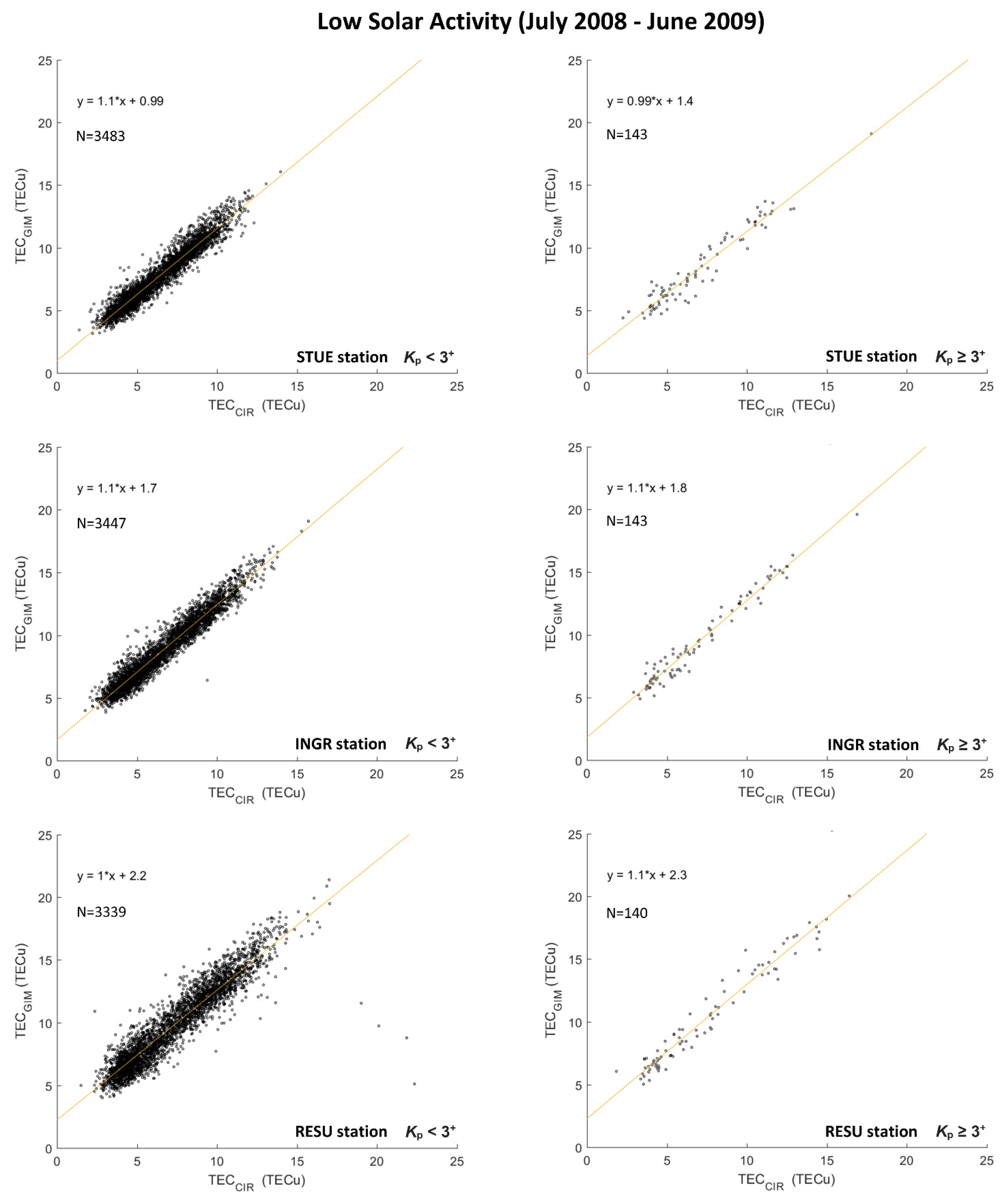
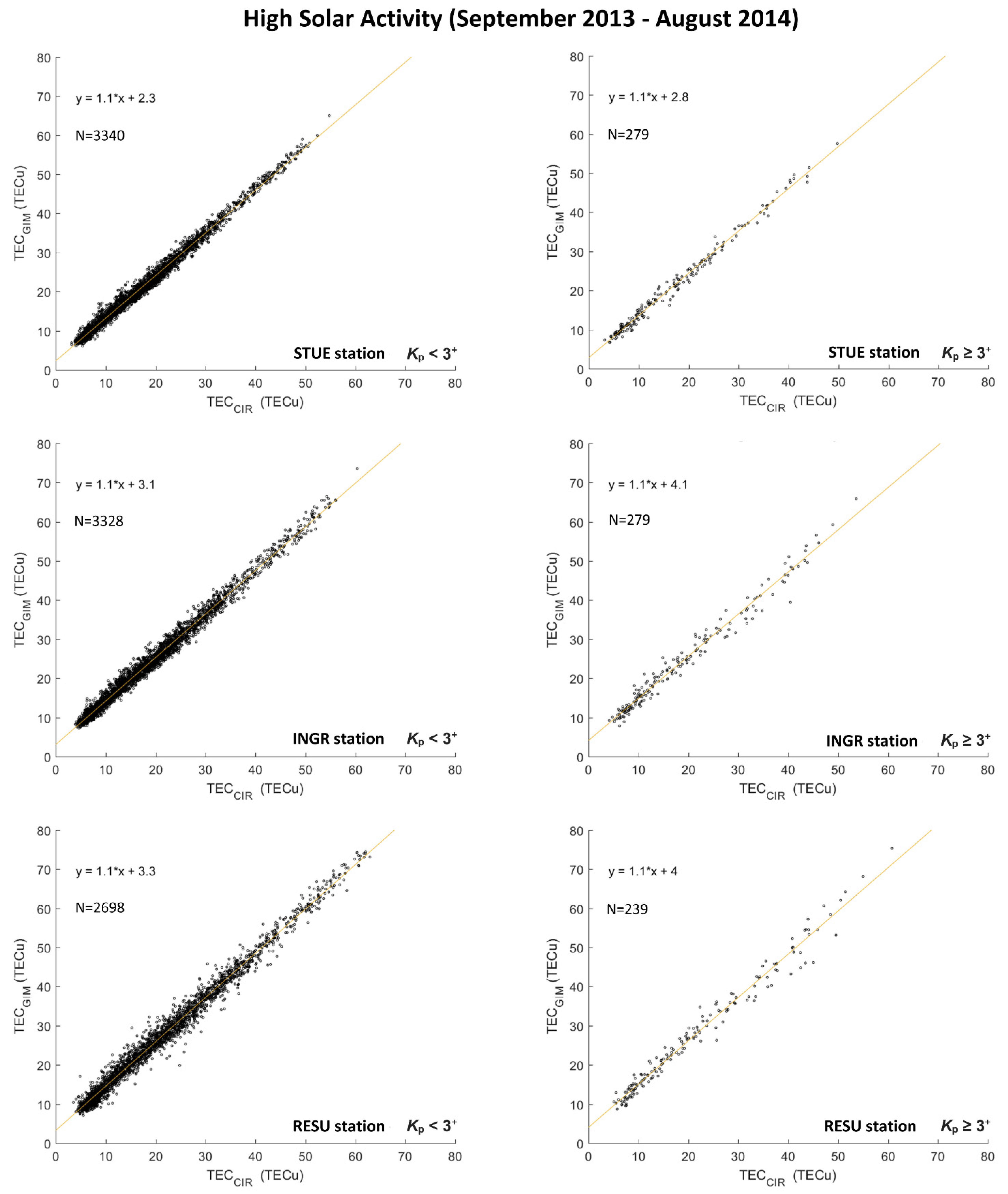
3. Results and Discussion

Scatterplots (TEC_GIM vs. TEC_CIR) for STUE, INGR, and RESU are shown for LSA and HSA periods in Figure 1 and Figure 2, respectively, distinguishing also between quiet (K_p < 3⁺) and disturbed (K_p ≥ 3⁺) geomagnetic datasets. Of course, the number of values related to disturbed conditions is much lower than the one characterizing quiet conditions because, usually, the number of geomagnetically disturbed days is by far lower than quiet ones. The number N of TEC values used in the study is shown inside each plot for all datasets.

These figures show that TEC_GIM values are always higher than TEC_CIR values, independently of solar activity, geomagnetic conditions and latitude, even though the correlation between the two datasets is really good (≥0.9) for all conditions, as it will be shown at the end of this section. This could be due to the different assumptions made for the DCBs estimation by IGS and Ciraolo algorithm. In fact, GIMs are calculated by forcing to zero the sum of all the satellites DCBs, while the Ciraolo algorithm assumes that β (see Equation (10)) is constant over each arc of observation. Moreover, Figure 1 and Figure 2 show that the difference between TEC_GIM and TEC_CIR values presents a latitudinal dependence; the intercept of the linear regression in fact shows that this difference increases from the north to the south of Italy. This issue is consistent with previous studies by Jee et al. [14] and Abe et al. [17], who found that TEC_GIM estimates are more reliable at mid-latitudes than at low latitudes, where the dynamics of the ionospheric plasma is much more complex to be modeled.

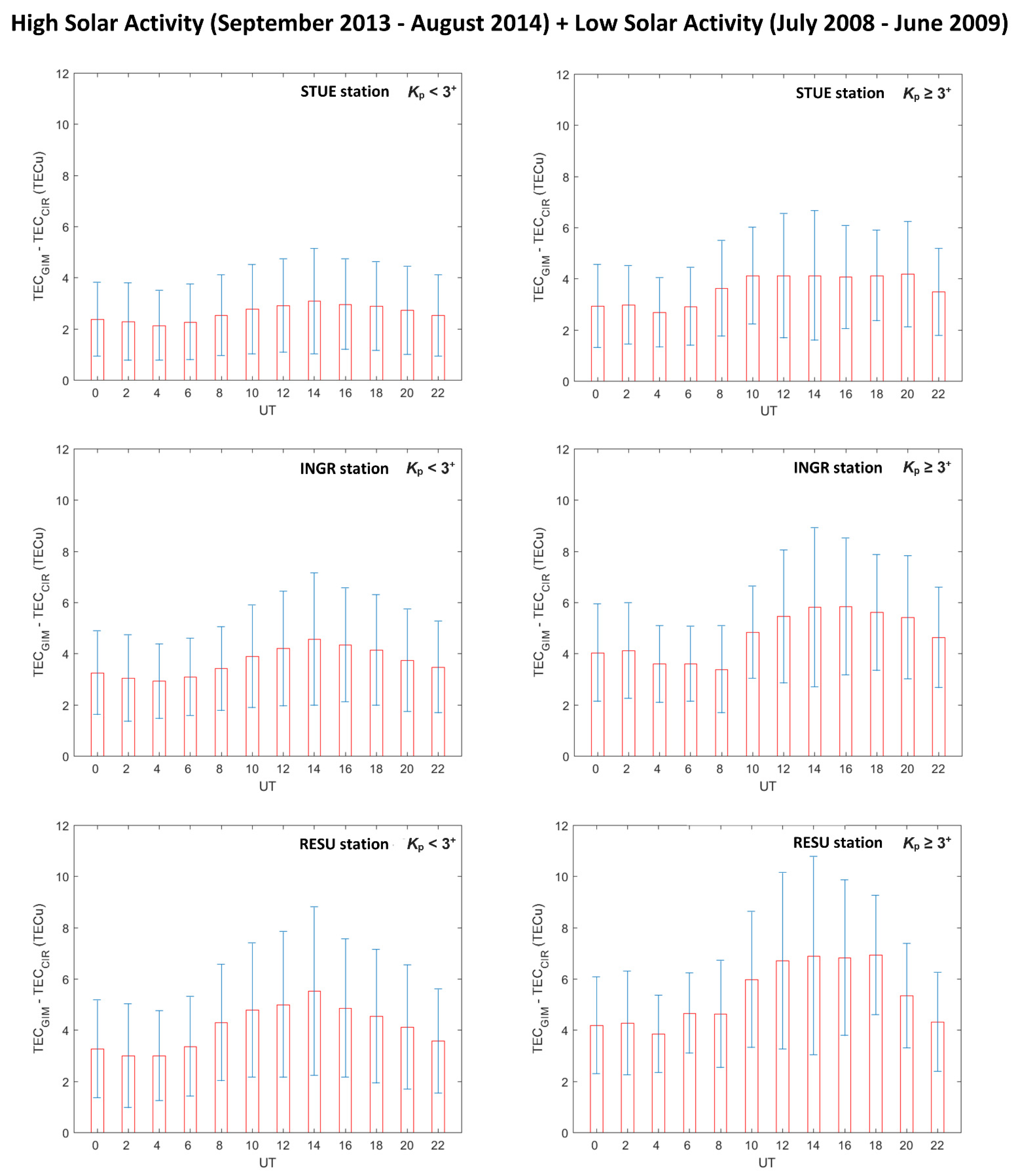
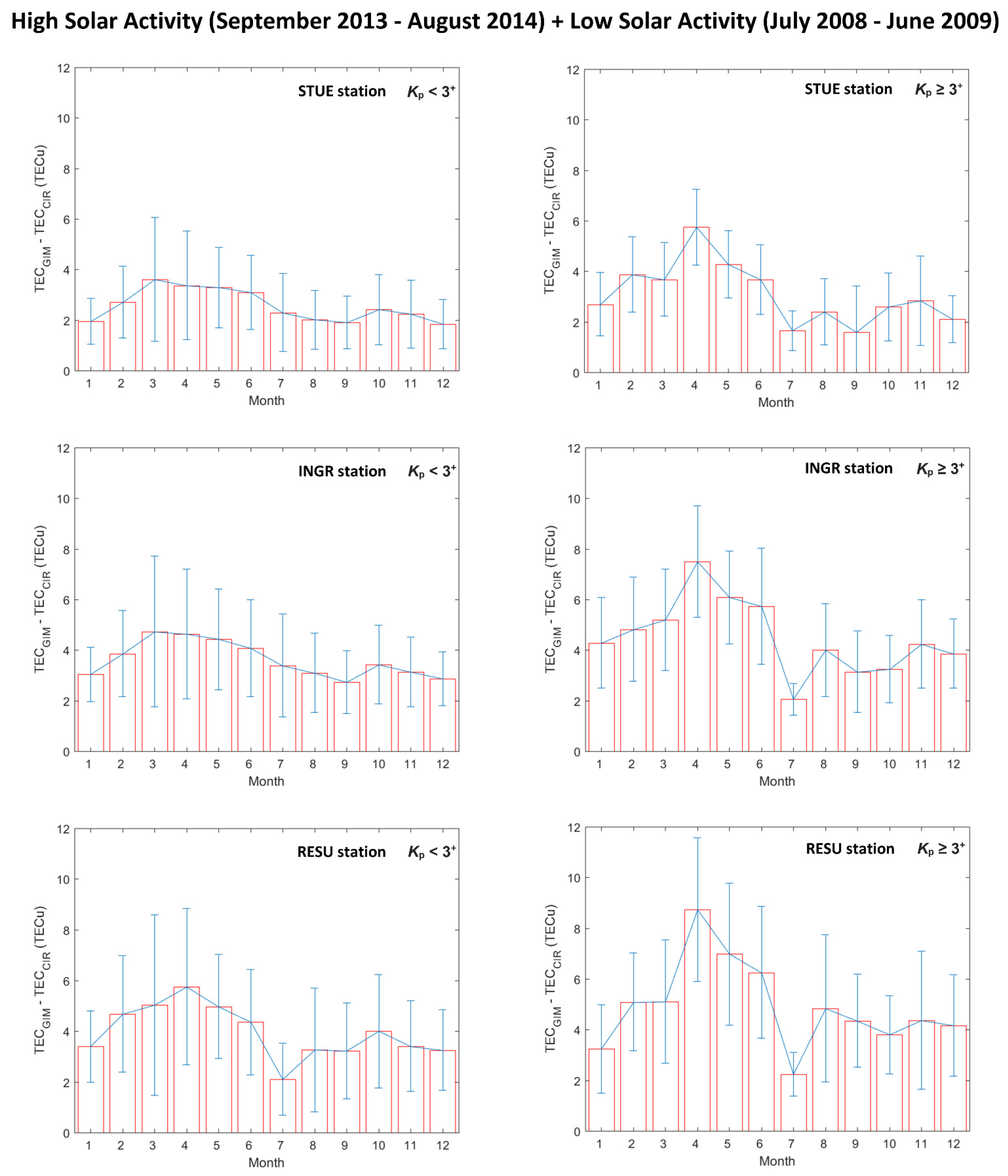
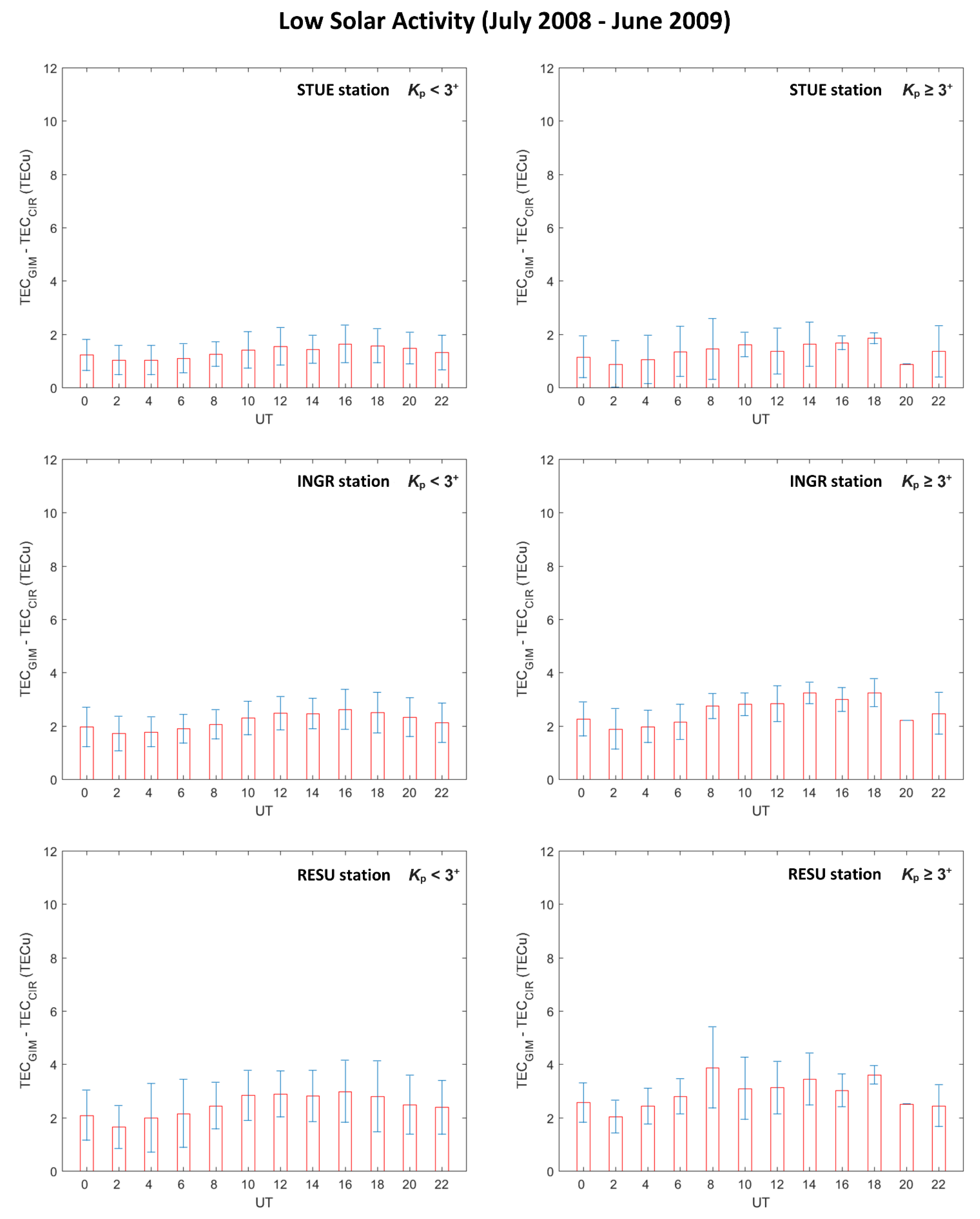
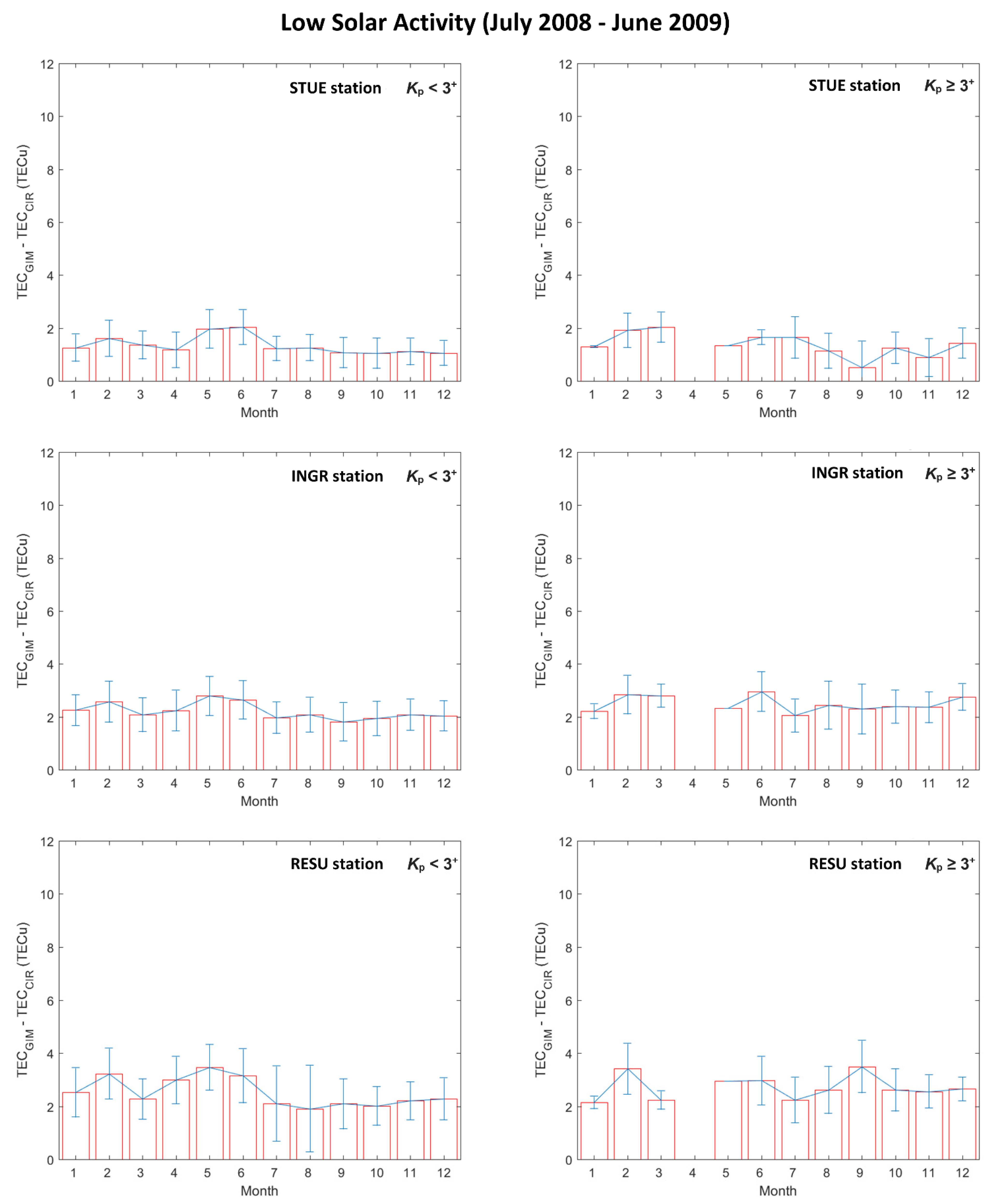
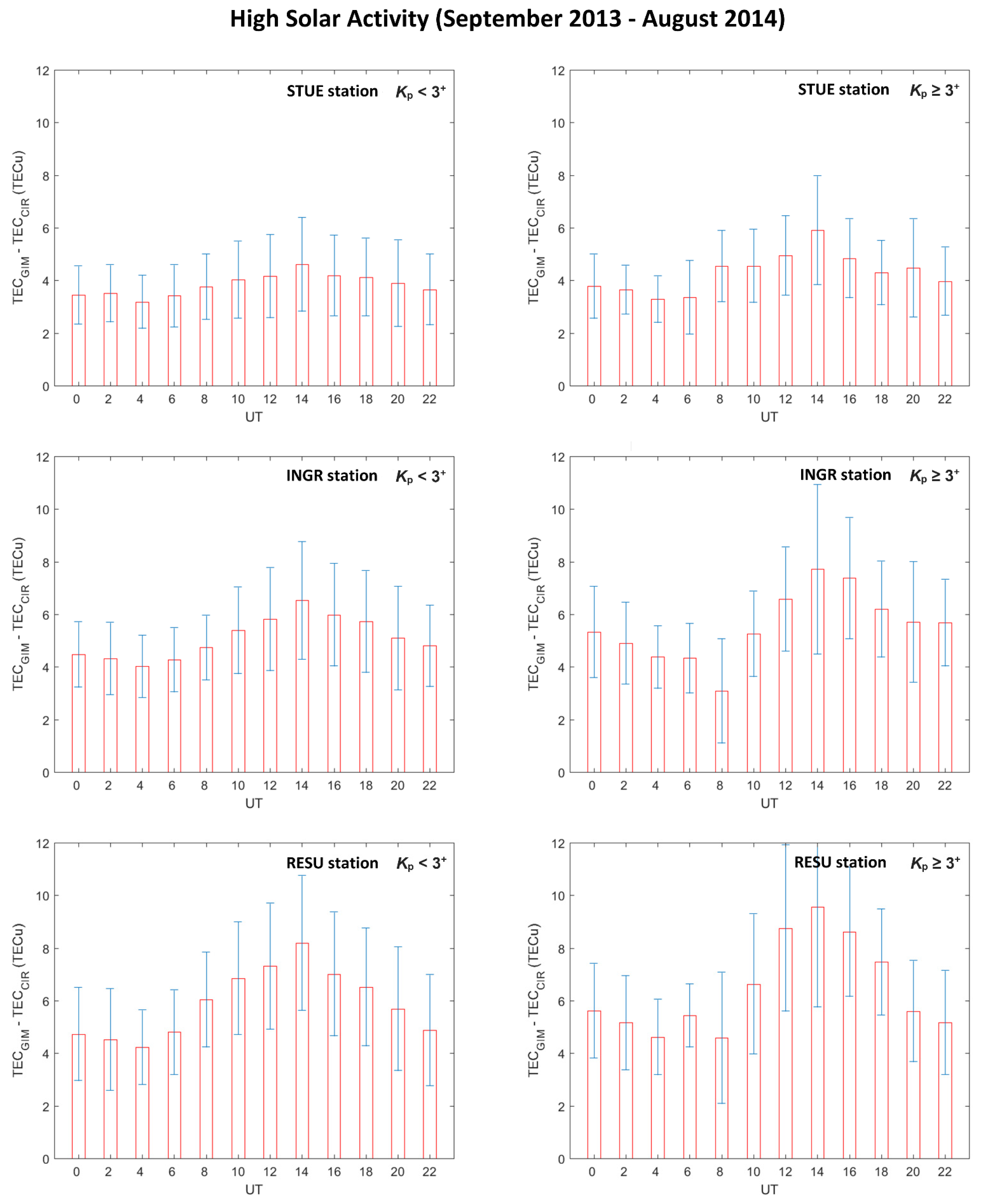
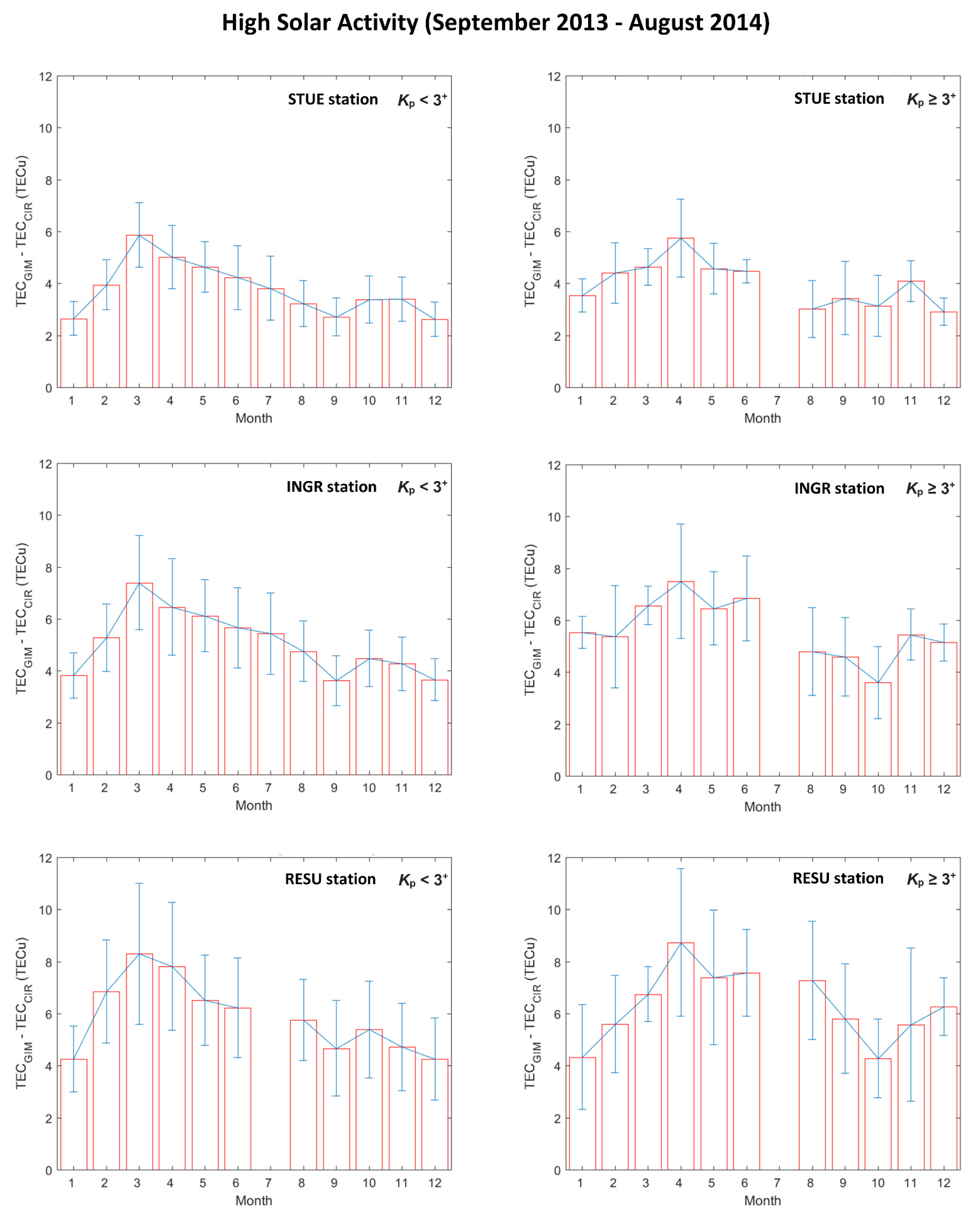
Additionally, the daily and seasonal dependence of the TEC differences obtained with the two methods has been investigated. Figure 3 and Figure 4 show for STUE, INGR and RESU the daily and monthly variations of the difference (TEC_GIM–TEC_CIR) with the corresponding standard deviation. Corresponding analyses are based on a joined HSA and LSA dataset and on averages of all values obtained respectively at 00, 02, …, 20, 22 UT (Figure 3), and for each month (Figure 4). Figure 5, Figure 6, Figure 7 and Figure 8 report the same analyses shown in Figure 3 and Figure 4 but considering the LSA and HSA dataset separately.

The difference (TEC_GIM–TEC_CIR) increases as the solar activity increases, confirming what was previously found by Jee et al. [14], who suggested a mismodeling of the plasmaspheric contribution by GIMs for high solar activity. Mean daily variation of the difference (TEC_GIM–TEC_CIR) is characterized by a maximum, which is reached at around 14 UT (see Figure 3); this feature is still visible when distinguishing between LSA and HSA (see Figure 5 and Figure 7). However, one would expect to obtain larger differences around solar terminator hours—when large electron density gradients take place—than around noon, when the ionospheric plasma can be considered almost stationary [32]. This might occur due to a GIMs mismodeling of a mid-latitude phenomenon known as meridian depression. The meridian depression is a peculiarity for which the daily absolute maximum of electron density is observed a few hours past the local noon; it has been recently renamed as Mid latitude Summer Evening Anomaly (MSEA) [33]. The main possible mechanism considered at the base of the meridian depression is the variation of the ratio [O]/[N₂], which increases from noon to midnight. Due to the longitudinal gradients of the [O]/[N₂] ratio, consistent longitudinal-dependent variations in the meridian depression magnitude may occur. This might represent mostly a problem for GIM’s generation that is based on global interpolation and less for the single site calibration method developed by Ciraolo et al. [17].

The mean monthly variation (see Figure 4, Figure 6 and Figure 8) is instead characterized by a double maximum of the differences around equinoxes, especially in spring, which is more pronounced for HSA. This is likely due to the semiannual anomaly characterizing the ionospheric plasma variability that is not always properly represented by GIMs, as highlighted by Mendillo et al. [34] and Zou et al. [35].

Moreover, Figure 3, Figure 4, Figure 5, Figure 6, Figure 7 and Figure 8 show that the differences between TEC_GIM and TEC_CIR are significantly affected by geomagnetically disturbed conditions. In fact, independently of solar activity, season, hour of the day, and latitude, the difference (TEC_GIM - TEC_CIR) increases for values of the geomagnetic index K_p ≥ 3⁺; this means that, for geomagnetic disturbed conditions, the method (either global or local) used to estimate TEC values has to be carefully selected.

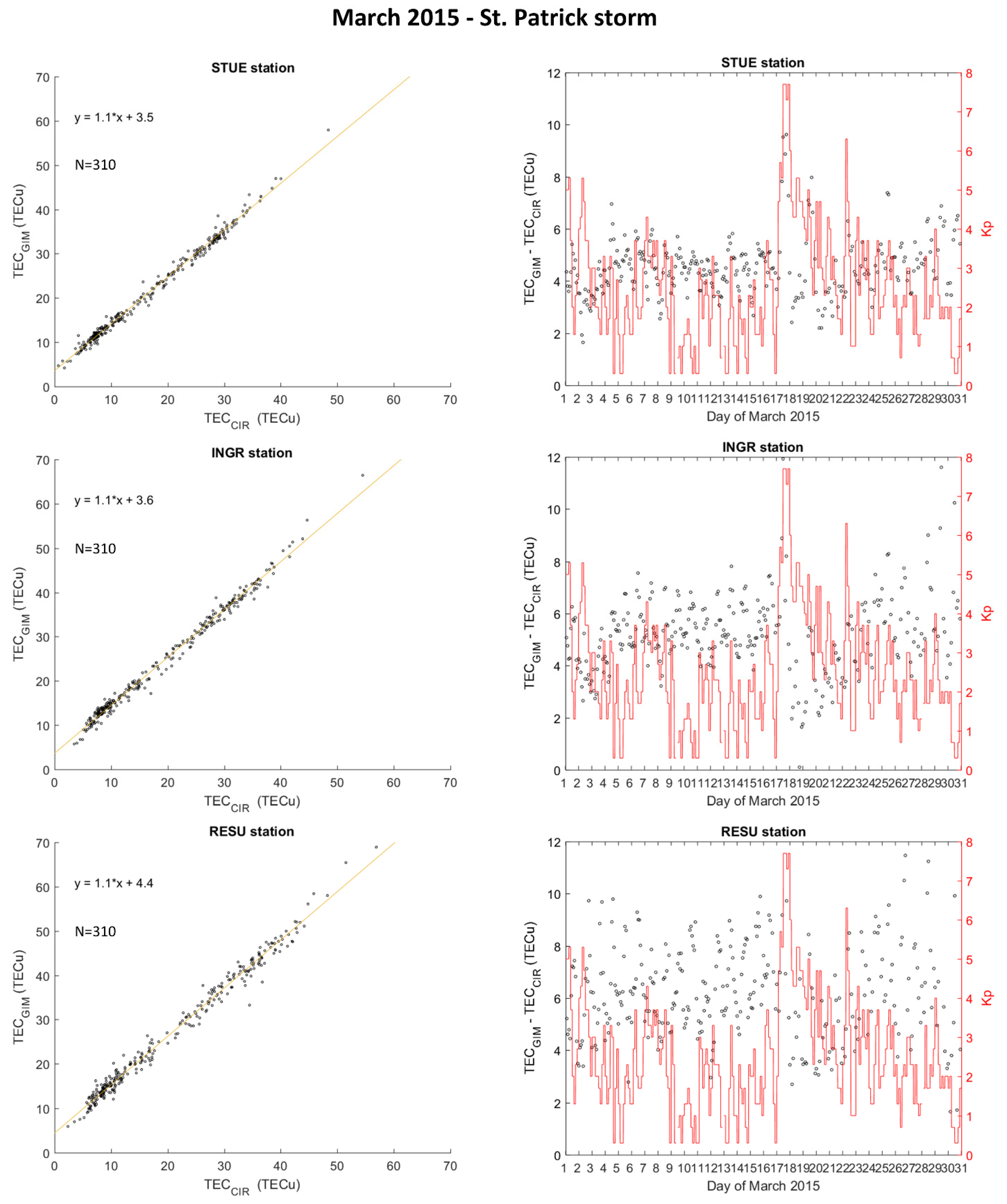
To further investigate this issue, we show in Figure 9 for STUE, INGR and RESU the scatterplots (TEC_GIM vs. TEC_CIR) and corresponding residuals (TEC_GIM–TEC_CIR) for the whole month of March 2015, which includes the well-known St. Patrick storm that occurred between 17 and 19 March 2015. Scatterplots are in line with those of Figure 2 obtained for HSA and disturbed conditions, but the most significant features shown by Figure 9 are the very large differences characterizing the March 17, as soon as the geomagnetic storm starts. During abrupt and strong geomagnetic variations, the GPS data processing is quite complicated. Specifically, in these conditions, the much more probable presence of ionospheric irregularities causes a higher number of cycle slips in carrier phases, which are difficult to be managed (e.g., Zhang et al. [36]). Therefore, during extreme geomagnetic conditions, it is hard to assess which method is the most suitable to be used.

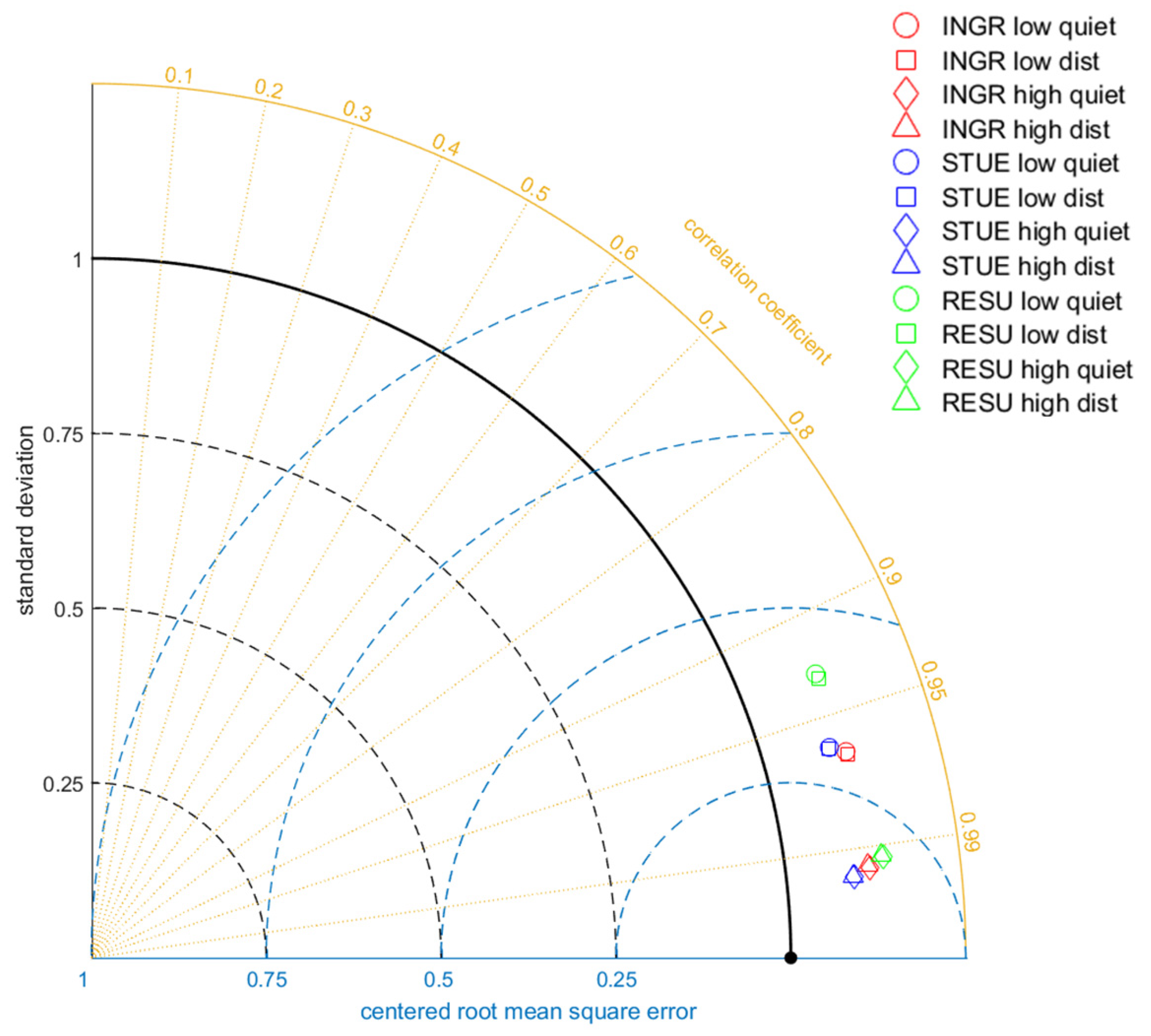
In order to summarize the main statistical features characterizing the difference (TEC_GIM–TEC_CIR) for the considered stations, under different solar and geomagnetic conditions, Figure 10 reports the Taylor diagram [37] for all the analyzed datasets. In this diagram, the y-axis represents the TEC_GIM standard deviation (SD) normalized to the TEC_CIR standard deviation (SD_CIR), the x-axis represents the normalized (or centered) root mean square error (NRMSE), and the circular axis represents the correlation coefficient R. This diagram has the peculiarity to represent three parameters in a two-dimensional plot, according to the following relation:

$$NRMS{E}^2=S{D}_{\mathrm{CIR}}^2+S{D}^2-2*S{D}_{\mathrm{CIR}}SD*R$$

(11)

Even though values of the difference TEC_GIM–TEC_CIR are higher for HSA, the highest precision (related to the standard deviation) and accuracy (related to NRMSE) of TEC_GIM is reached during HSA, for both quiet and disturbed conditions. This feature slightly degrades moving from north to south. For LSA, it can be noted that the accuracy is considerably lower in the southern station RESU.

4. Summary and Conclusions

In this study, we evaluated the performance of TEC values obtained both by IGS GIMs and calibrated applying the Ciraolo et al. [17] technique over three permanent GPS RING stations in Italy: STUE, INGR and RESU, located respectively in the north, center and south of Italy. Results have been compared for both low and high solar activity. Specifically, the considered periods were those between July 2008 and 2009 for LSA, and between September 2013 and August 2014 for HSA. Moreover, the considered dataset has been differentiated also in terms of the geomagnetic index K_p to assess separately the disturbed periods (K_p ≥ 3⁺) from the quiet ones (K_p < 3⁺). Concerning the disturbed conditions, the period of March 2015, including the severe St. Patrick geomagnetic storm occurrence on 17–19 March 2015, has also been considered. TEC_CIR values obtained through the Ciraolo et al. [17] method have been calibrated using RINEX files recorded every 30 s at STUE, INGR and RESU. After performing the calibration, a 5 min running mean has been applied to smooth out any possible spike characterizing the time series. Finally, to be consistent with the 2 h time resolution of GIMs, for each day of selected periods, values corresponding at 00, 02, …, 20, 22 UT have been considered.

According to the main outcomes of the study, TEC_GIM and TEC_CIR values are highly correlated, but TEC_GIM values are always greater than TEC_CIR values, independently of solar and geomagnetic activity, hour of the day, season and latitude. This could be ascribed to the different assumptions made for the DCB estimation by IGS and Ciraolo algorithm. Anyhow, the difference (TEC_GIM–TEC_CIR) significantly increases as the solar activity increases. With regard to this, it has to be considered that during HSA periods there is an increase of the solar extreme ultraviolet radiation, with a consequent intensification of electric fields in the upper atmosphere; this fact, for instance, increases the vertical E × B drift (where E is the equatorial zonal electric field and B the geomagnetic field) at low latitudes, with a consequent enhancement of the growth of instability processes like the Rayleigh-Taylor one, which are at the base of the ionospheric irregularities formation [38,39]. Therefore, the increased difference (TEC_GIM–TEC_CIR) for HSA could mean that GIMs find it more difficult to manage the corresponding growth of ionospheric irregularities.

Moreover, the difference (TEC_GIM–TEC_CIR) is higher for geomagnetic disturbed conditions than for geomagnetic quiet ones, especially during the early phase of a geomagnetic storm when very large values are obtained. This difference is also affected by a latitudinal dependence, increasing from the north to the south of Italy. This confirms the results found by previous studies [14,17], which found that GIMs are more reliable at mid-latitudes than at low-latitudes.

From the Taylor diagram it can be concluded that although (TEC_GIM–TEC_CIR) differences are higher for HSA, the corresponding relative errors are lower than those characterizing LSA.

The results shown in this paper highlight that, since they are computed at a global level, TEC GIMs might have to be used carefully at a regional level. In fact, in the case of the Italian region, only eight Italian IGS stations are used to generate GIMs, with quite long reciprocal baselines (of about hundreds of km). This outcome is especially true for those scientific studies, focused on mid-latitude ionospheric irregularities, traveling ionospheric disturbances and lithosphere-ionosphere coupling, for which a high degree of accuracy is requested to properly represent the ionospheric dynamics.