Article

Advection Fog over the Eastern Yellow Sea: WRF Simulation and Its Verification by Satellite and In Situ Observations

1
Korea Institute of Atmospheric Prediction Systems, Seoul 07071, Korea
2
School of Earth and Environmental Sciences, Seoul National University, Seoul 08826, Korea
3
Korea Institute of Ocean Science and Technology, Busan 49111, Korea
*
Author to whom correspondence should be addressed.
Submission received: 3 March 2021 / Revised: 2 April 2021 / Accepted: 7 April 2021 / Published: 12 April 2021
(This article belongs to the Special Issue Use of Remote Sensing for High Impact Weather)

Abstract

:
An observed sea fog event over the Eastern Yellow Sea on 15–16 April 2012 was reproduced in the Weather Research and Forecasting (WRF) simulation with high-resolution to investigate the roles of physical processes and synoptic-scale flows on advection fog with phase transition. First, it was verified by a satellite-based fog detection algorithm and in situ observation data. In the simulation, longwave (infrared) radiative cooling (LRC) with a downward turbulent sensible heat flux (SHF), due to the turbulence after sunset, triggered cloud formation over the surface when warm-moist air advection occurred. At night, warm air advection with continuous cooling due to longwave radiation and SHF near the surface modulated the change of the SHF from downward to upward, resulting in a drastic increase in the turbulent latent heat flux (LHF) that provided sufficient moisture at the lower atmosphere (self-moistening). This condition represents a transition from cold-sea fog to warm-sea fog. Enhanced turbulent mixing driven by a buoyancy force increased the depth of the sea fog and the marine atmospheric boundary layer (MABL) height, even at nighttime. In addition, cold air advection with a prevailing northerly wind at the top of the MABL led to a drastic increase in turbulent mixing and the MABL height and rapid growth of the height of sea fog. After sunrise, shortwave radiative warming in the fog layers offsetting the LRC near the surface weakened thermal instability, which contributed to the reduction in the MABL height, even during the daytime. In addition, dry advection of the northerly wind induced dissipation of the fog via evaporation. An additional sensitivity test of sea surface salinity showed weaker and shallower sea fog than the control due to the decrease in both the LHF and local self-moistening. Detailed findings from the simulated fog event can help to provide better guidance for fog detection using remote sensing.

Graphical Abstract

1. Introduction

Fog is defined as clouds near the surface with a horizontal visibility less than 1 km due to microscopic droplets or ice crystals that stay near the surface boundary layer [1]. In particular, fog formed over the ocean, called sea fog, is denser and formed in large areas due to high relative humidity (RH) mainly caused by the ocean. Thus, it persists over the ocean because it moves slowly according to the wind and it is difficult to dissipate. Analysis of sea fog events is important to provide safe and efficient operations in aviation, marine, and road transportation. In addition, these events have an impact on trapping atmospheric pollutants by forming the lower layer with strong temperature inversion while the fog prevails [2,3]. Sea fog is generally classified as advection fog or steam fog [4]. Advection fog is formed through air movement over an ocean surface with a different temperature, and frequently occurs in many regions where a temperature difference between the ocean and the air exists, such as off the coast of southern California, U.S. West Coast, Arctic region, and Yellow Sea [1,4,5]. It includes warm-sea fog and cold-sea fog phases. Warm-sea fog is frequent in spring when colder air is flowing over a warmer ocean, but cold-sea fog is dominant in summer because the ocean surface temperature (Ts) becomes generally cooler than the air temperature (Ta) [5,6,7,8]. In particular, steam fog is formed when advected air becomes much colder than Ts, and it is frequently observed in the Arctic regions [9] due to the fact that Ts (with a range of −1 to 3 degrees Celsius in winter) is considerably warmer than Ta and thus the difference between Ts and Ta becomes about 15–20 °C, which is confined by strong inversion at the top [3,4,9]. Due to the formation of a significantly warmer ocean, steam fog events are less frequent than advection fog events. All of these fogs are dissipated by an increase in atmospheric instability due to warming of the lower atmosphere by sunrise and/or a strong wind shear and by an increase in evaporation due to low relative humidity.
The Yellow Sea between China and the Korean peninsula is a region in which sea fog frequently occurs (Figure 1). It is understood that warm-sea fog and cold-sea fog events are generally frequent in spring and summer, respectively, over the Yellow Sea of the Korean peninsula [5,6,7,8]. Accurate prediction of the formation, evolution, and dissipation of sea fog is highly challenging because the difference between Ts and Ta is dynamic, depending on variations in synoptic conditions and ocean currents. Some studies have also emphasized that sea fog is influenced by the synoptic conditions, in addition to local meteorological conditions near the surface [4,8,10]. The mechanism of cold-sea fog has been studied extensively, and recently more efforts have focused on warm-sea fog, which accounts for more than 30% of total advection fog in the western Yellow Sea [5]. Previous research found, using observation and reanalysis data, that in the transition from cold-sea fog to warm-sea fog, longwave (infrared) radiation cooling (LRC) at the top of the surface fog layer plays an important role, and synoptic-scale subsidence pushes down the marine atmospheric boundary layer (MABL) [5]. In particular, the synoptic conditions near the Korean peninsula in spring can change immediately between cold/dry and warm/moist air flows, which result in the occurrence of a transition between cold-sea fog and warm-sea fog (a mixed type of cold-sea and warm-sea fog). For the eastern Yellow Sea, clearer understanding is required for the formation, evolution, and dissipation of advection fog events with the transition of the difference between Ts and Ta (Ts–Ta), in accordance with the MABL and underlying background conditions. To fully understand the mechanism for a mixed type of cold-sea and warm-sea fog in different areas, additional case studies of multiple vertical layers in the MABL are required.
Numerous attempts have been made to study the detection or mechanism of sea fogs using both observations and numerical simulations. For example, an algorithm for a warm fog detection using a combination of Geostationary Operational Environmental Satellite-12 (GOES-12) observations and screen temperature data based on a Canadian operational numerical model was developed [11]. They suggested that the detection of the warm fog from the satellite-based algorithms can be improved by including model-based sounding values. A parameterization scheme for warm-sea fog visibility was introduced using in situ observations and combined parameters such as droplet number concentration and liquid water content from a numerical weather prediction model [12]. Besides, it was found that the uncertainty of Arctic clouds decreased by considering the origin of the air mass using air-mass back trajectories calculated from the numerical model outputs [13] and that the simulation using a three-dimensional cloud-resolving model with explicit bin-resolving cloud microphysics can reproduce the atmospheric boundary layer and cloud evolution associated with the polynya [3]. All these previous studies suggested that numerical models are important factors for the accurate detection and mechanism of fog or low-level clouds [12].
Some studies revealed the physical properties of fogs or stratiform clouds using numerical prediction models and observed data [14,15]. One found that cloud microphysical properties are significantly different for the ocean and land cases and clouds in the sub-grid scales can be better represented in the simulation using probability distribution curves for microphysical or optical parameters [14]. The other found that sea fog is formed by the turbulent exchange of heat and moisture, the diurnal variation in radiation, and advected air flows over the sea surface, and that turbulent heat and moisture fluxes modify the environment of temperature and humidity within the MABL [15]. They also mentioned that the ascent of the fog top may be related to the turbulence that enhances the entrainment mixing of the relatively humid air from above the fog top [15]. According to previous studies, understanding the physical processes such as radiation, microphysics and turbulence for the formation and dissipation of fog is essential, and it is expected that turbulence in the MABL, which has a close interaction with radiation and advection processes, plays an important role during the duration of the formation and dissipation of the sea fog. Meanwhile, few efforts have been made to uncover the physical mechanisms for the mixed type of cold-sea and warm-sea fog in previous studies.
This study aimed to understand the mechanisms of the formation, evolution, and dissipation for the mixed type of cold-sea and warm-sea fog (in particular, a transition of cold-sea to warm-sea fog) over the eastern Yellow Sea, using high-resolution numerical simulation. In particular, this study attempted to understand five factors: (1) the impact of the change in temperature and moisture due to turbulent fluxes, radiative fluxes, and thermal and moisture advection on the formation and dissipation of sea fog; (2) the role of the change in synoptic-scale flows (e.g., transition from warm/moist advection to cold/dry advection) in the growth of the MABL; (3) the influence of the resulting MABL evolution on the vertical diffusion of fog due to turbulence intensified by mechanical and buoyant forcing; (4) the dependency of the mechanisms of sea fog on the regions; and (5) the impact of sea surface salinity on simulated sea fog. For this purpose, we investigated the mechanisms of sea fog with their related physical processes, focusing on the interactions between the surface turbulent flux, MABL height, and tendencies of temperature, water vapor (Qv), and cloud liquid water content (Qc), using a numerical simulation of a sea fog during the spring season. This paper is organized as follows: Section 2 describes the model and experimental design. Synoptic-scale flows and spatial distributions of sea fog from satellite and sounding observations, and a WRF simulation, and a brief description of the selected events, are examined in Section 3.1 to examine the performance of the model for the mixed type of cold-sea and warm-sea fog. Relevant physical processes, in particular the process associated with turbulence, in terms of the formation, evolution, and dissipation, are discussed in Section 3.2. In addition, a sensitivity test of salinity effect is also examined in this section. Finally, conclusions are outlined in Section 4.

2. Model and Experimental Design

The WRF model version 4.0 was used for the sea fog case simulation [16]. This study focused on a sea fog event over the eastern Yellow Sea. The experiment had four nested domains, including the East Asian region centered over the eastern Yellow Sea of the Korean Peninsula, with horizontal resolutions of 27, 9, 3, and 1 km (Figure 1). It employed 51 vertical eta levels with a model top of 50 hPa, of which 15 layers were located at the lower atmosphere below about 950 hPa because a sea fog event usually occurs near the surface. Physical schemes employed in this study included the Yonsei University (YSU) boundary layer scheme [17], the WRF double-moment 6-class microphysics scheme (WDM6) [18], the Rapid Radiative Transfer Model (RRTM) for the radiation scheme [19], the unified Noah land surface model [20,21,22], and the revised MM5 Monin–Obukhov surface layer scheme [23]. The Kain–Fritsch cumulus parameterization scheme [24] was used only for domains 1 and 2.
The sea fog event observed by satellite data over the Yellow Sea of the Korean peninsula on 15–16 April 2012 was selected in this study. The simulation was carried out for 36 h forecasts initiated at 0000 UTC 15 April 2012. The initial atmospheric and bottom boundary conditions were taken from the National Centers for Environmental Prediction (NCEP) Global Forecast System Final Analysis (GFS-FNL) dataset with 1° × 1° spatial resolution, and the optimal interpolation sea surface temperature (OISST) with 0.25° × 0.25° spatial resolution, respectively. For boundary conditions in the child domains, one-way nesting domains were used. Details for the experimental setting of the WRF model and the configuration of the physics package are given in Table 1 and Table 2, respectively.

3. Results

3.1. Case Overview

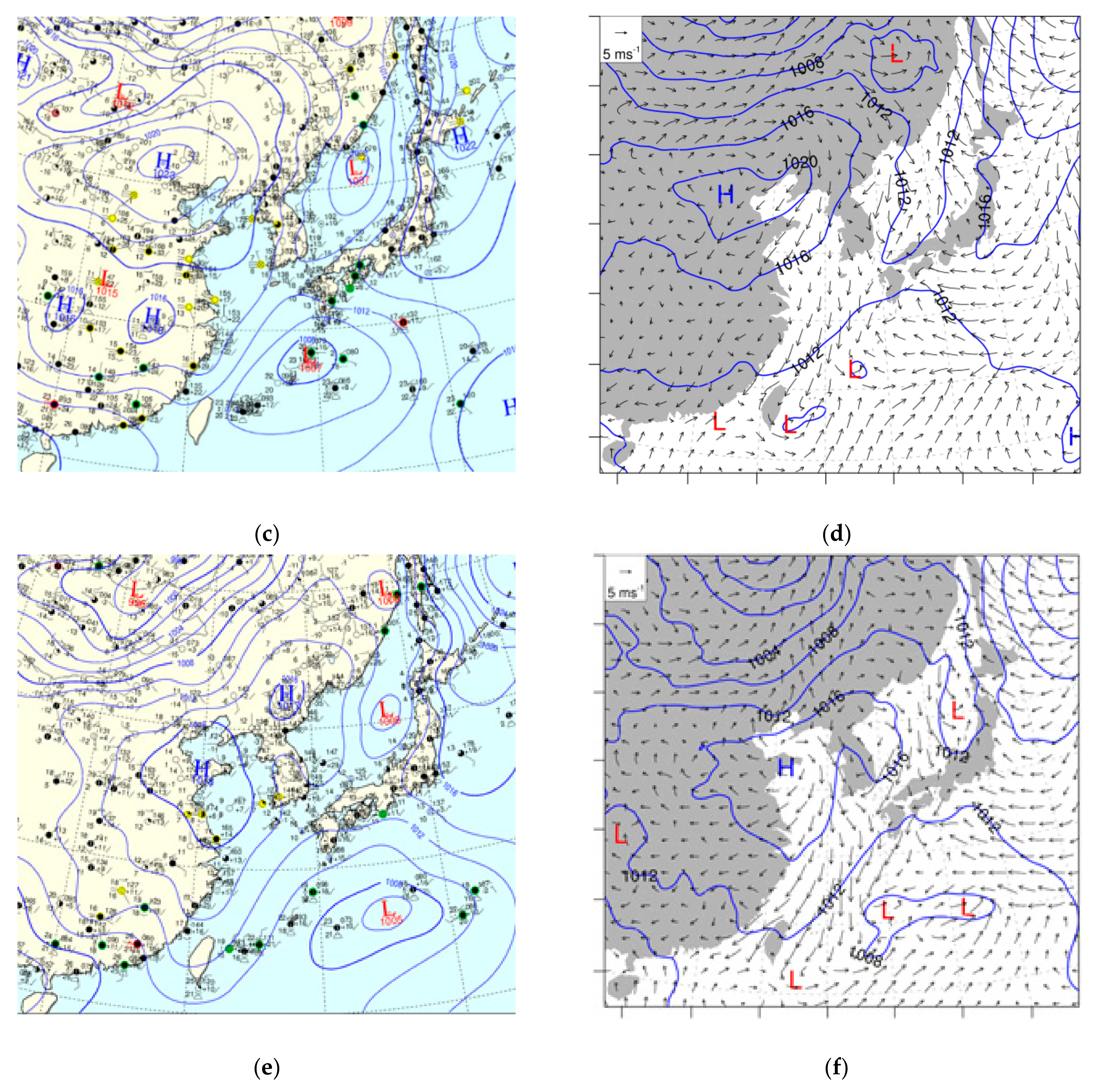
3.1.1. Synoptic-Scale Flows

Figure 2 shows the horizontal distributions of mean sea level pressure with a 10 m wind at 1200 UTC (2100 KST) and 0000 UTC (0900 KST) on 15 April 2012, and 1200 UTC on 16 April 2012, obtained from the Korea Meteorological Administration (KMA) and simulated by the WRF model. On 15 April 2012, a local high-pressure system, which originated from the Siberian high-pressure system centered at central China, was separately located in the south-western region of the Yellow Sea of the Korean peninsula, and a weak low-pressure system was located in Wonsan Bay in eastern Korea. Thus, it could be expected that the west coast of Korea was affected by a weak south-westerly wind with a weak pressure gradient. It was found that the northern parts of the Yellow Sea were affected by warm and moist air flows under this synoptic condition (Figure 2a). Then, the synoptic-scale fields changed at 0000 UTC 16 April because the continental high-pressure system in north China quickly expanded to the northern Yellow Sea. This led to a high-pressure system to the north of Korea and a low-pressure system to the south of Korea at this time (Figure 2c). Therefore, it induced a cold and dry air flow due to the presence of northerly winds. The synoptic-scale conditions with northern winds were maintained until 1200 15 April 2012 (Figure 2e).
In the spatial patterns of the simulated mean sea level pressure shown in Figure 2b,d,f, it can be seen that synoptic-scale conditions shown in the analytical surface weather chart were reproduced correctly in the simulation. In detail, the high-pressure system to the west of the Korean peninsula and the low-pressure system to the east of the Korean peninsula, and the south-westerly wind, were consistent with the simulated result at 1200 UTC on 15 April 2012. Then, at 0000 UTC on April 16, the continental high-pressure system centered at north China expanded to the western region of Korea, and the low-pressure system was located in the southern part of the Korean peninsula. Subsequently, the western part of the Korean peninsula was dominated by the anticyclonic flow due to the movement of the high-pressure system. Overall, it was expected that the synoptic-scale conditions at 1200 UTC on 15 April 2012 and 0000 UTC 16 April 2012, in both analytical and simulated surface weather charts, supported the fine weather conditions during this period. According to the skew T-Log P diagram (Figure 2g) and simulated wind near the surface (Figure 2b,d,f), the change of wind direction from southerly to northerly. Thus this case had good synoptic-scale conditions with a change from a warm/moist air flow to a cold/dry air flow for the formation of both cold-sea fog and warm-sea fog, in which the air–sea interaction met the formation of the cloud near the surface. Eventually, the transition of the cold-sea fog to a warm-sea fog could occur under these conditions. The distribution of the sea fog observed by satellite data is presented in the next section.

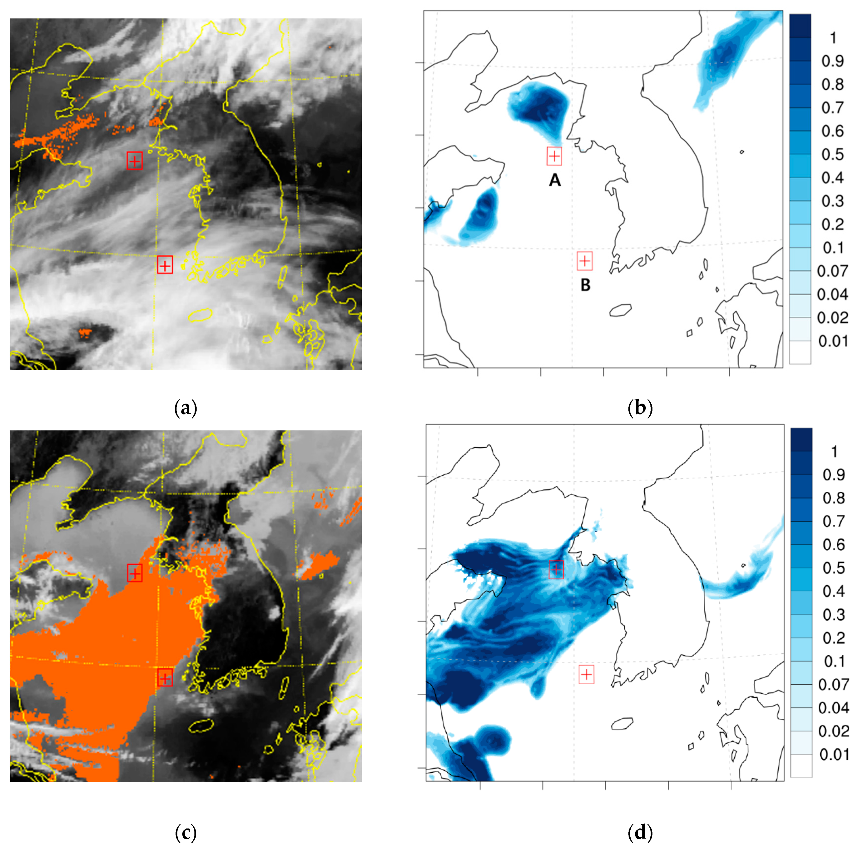
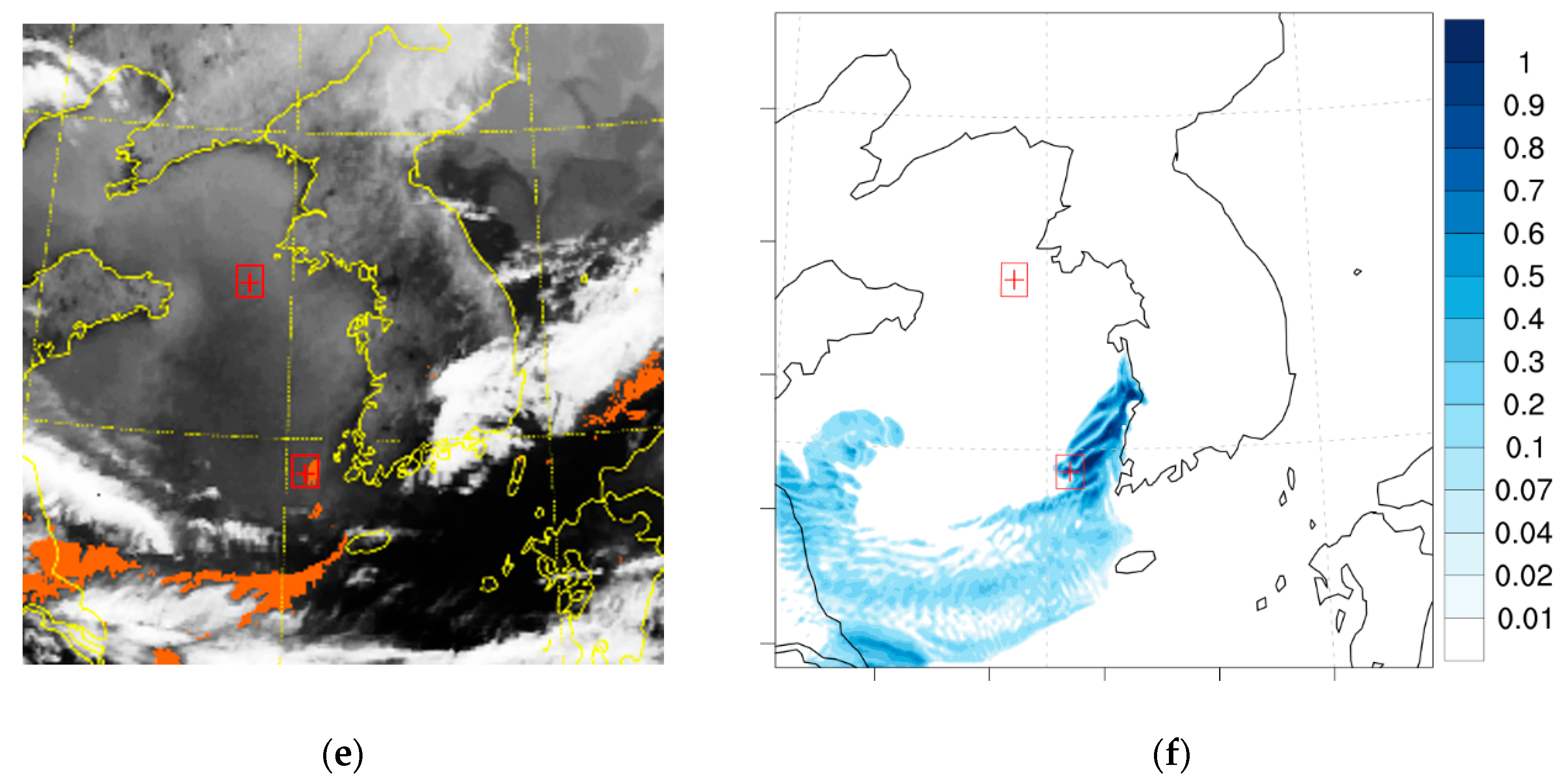
3.1.2. Distribution and Verification of Sea Fog

To verify sea fog simulated from the WRF model, the spatial distribution of sea fog from the observed data and simulation were compared. Figure 3a,c,e depict near-infrared images obtained from the Communication, Ocean and Meteorological Satellite (COMS) operated by the National Meteorological Satellite Center of Korea (https://nmsc.kma.go.kr/homepage/html/main/main.do; accessed on 1 August 2020) at 1200 UTC on 15 April 2012, and 0000 UTC and 1200 UTC on 16 April 2012, which can detect the spatial distribution of fog, expressed with an orange color. In the COMS images, a fog area is defined by using the visible channel reflectance during the daytime and by using the difference in brightness temperature between the shortwave infrared channel and the infrared 1 channel during the other times. For the fog area, the surface temperature (maximum value of the brightness temperature of 1 infrared channel for 15 days) and the cloud top temperature were compared, and the difference was detected as the final fog when the difference was within 0~10 °C. The smaller the temperature difference, the more likely it is a fog area (http://www.weather.go.kr/weather/observation/marine_foq.jsp; accessed on 1 August 2020). It was shown that sea fog began to form over the northern part of the Yellow Sea after sunset at 1200 UTC 15 April 2012 (Figure 3a). Then, the fog gradually developed at night, with an extension to the southeast; consequently, it covered the entire part of the Yellow Sea between China and Korea at 0000 UTC 16 April (Figure 3c). This image showed that the event was a suitable case for the investigation of sea fog because cumulus or cirrus clouds on top of the fog layer were not observed when there was a large fog patch over the Yellow Sea. The fog was almost dissipated in most regions, leaving only a small portion in the south of the Yellow Sea at 1200 UTC 16 April 2012 (Figure 3e). Regarding the presence of sea fog, it was also confirmed in the surface weather chart (Figure 2a,c) that the weather symbol for fog (yellow shading at a designated station model) was reported at Baeknyeong island (the location is depicted as the red cross at “A” in Figure 3b) at 1200 UTC on 15 April and 0000 UTC on 16 April 2012, while it was also reported at Heuksan Island (the location is depicted as the red cross at “B” in Figure 3b) at 1200 UTC 16 April 2012 (Figure 2a,c,e). The distribution of the average of the simulated Qc for the levels below z = 100 m for domain 3 is plotted as blue shading in Figure 3b,d,f. Sea fog in the simulation was inferred through the areas with an average Qc higher than 0.01 g kg−1. The locations of A and B, marked with red-cross signs in the figures, refer to the stations at Baeknyeong and Heuksan islands, respectively. It can be observed that the spatial distribution of the sea fog was well simulated in the WRF model, although it showed a local discrepancy in slow occurrence or slow movement in some areas.
Figure 4 shows the evolution of vertical profiles (time–height cross-sections) of the simulated relative humidity (RH; top panel) and Qc (bottom panel) averaged within the 50 × 50 km areas centered at regions A and B. The simulated MABL height at each region is superimposed in Figs. 4a and b. In region A (Figure 4a,c), formation of the fog begins to form at the near-surface layer at 1200 UTC on 15 April, and the height of the fog gradually increases with time, and then the maximum height of the fog is shown in early morning at around 2200 UTC on 15 April 2012. Finally, it started to dissipate above the MABL. To verify the simulated sea fog, the top heights of the observed sea fog estimated from Meteorological SATelite-2 (MTSAT-2) geostationary satellite data were superimposed in Figure 4c,d, following the method mentioned in a previous study [12]. To detect nighttime sea fog, the difference in brightness temperatures between the 3.8 and 10.8 µm channels in the MTSAT-2 satellite data was determined [25,26]. The fog-top height was estimated from a function of the difference between the two channels for water clouds with a median drop diameter of 8 μm and a cloud temperature of 240 K, suggested in previous studies [26,27]. The brightness temperature difference between two channels increases as the thickness of water clouds increase. Note that satellite-based warm fog detection based on the algorithms using satellite data had an accuracy of less than 60% and the algorithms based on only brightness temperature difference between channels could not work accurately when an elevated fog layer occurred [11]. Accordingly, although the sea fog was shown in region A from the MTSAT-2 fog-top results, the presence of sea fog was unclear from 0000 UTC to 0700 UTC 15 April according to the weather charts. Thus, this study focused on the sea fog event over the eastern Yellow Sea during the period from 1000 UTC 15 to 1200 UTC 16 April. Observed sea fog was well simulated in the numerical model experiment during the sea fog event, although overestimation of the top heights was found in the simulation. The formation and dissipation phases of the sea fog estimated from the MTSAT-2 occurred at about 1200 UTC on 15 April 2012 and 0400 UTC on 16 April 2012, respectively. A somewhat earlier formation and delayed dissipation of sea fog was found in the simulation. However, it can be understood that the formation and dissipation timings were predicted well in the numerical model experiments. In region B (Figure 4b,d), unlike in region A, at 04 UTC on 16 April 2012 the sea fog started to form at a height of about z = 200 m with a low RH, whereas that in region A was formed from the surface with a sufficiently high RH. Thus, it can be expected that mechanisms for sea fog depend on the regions. Detailed mechanisms are discussed in the next section. Consequently, we can investigate the mechanisms for the sea fog from the numerical simulation, because both spatial and temporal distributions of the observed sea fog event were reproduced accurately in the model.
Figure 5 shows the vertical profiles of temperature and humidity simulated in the numerical model with the observed sounding data. In general, the simulated temperature and humidity at the time when the sea fog was dominant at the two stations showed good agreement with the observed data. In particular, at region A (Baeknyeong Island) the temperature profile simulates an inversion layer between 200 and 400 m, and it can be inferred that the condensation layer formed below it (i.e., the fog layer) will be trapped. Although there is a slight difference in the humidity profile, it has the maximum value in the lower layer and gradually decreases from the height at which the inversion layer begins, which is similar to that observed. The fog-top height in the numerical model increased to more than 300 m, whereas those inferred from the sounding data and from the MTSAT-2 were limited to about 200 m during the duration of the fog event. Note that the depth of the sea fog tended to be overestimated as reported in the current numerical simulation, which was somewhat consistent with previous studies [28,29,30,31].

3.2. Mechanism of Sea Fog

To understand the mechanisms of the sea fog, we investigated related physical processes in the stages of formation, evolution (growth and vertical jump), and dissipation at each of regions A and B.

3.2.1. Formation Stage

We first investigated the changes of temperature and hydrometer at the surface and the lowest model level (z1), because the formation of sea fog in region A started near the surface. The time series of surface turbulent fluxes and the MABL height in region A at the formation and evolution stages are displayed in Figure 6. The positive (negative) turbulent fluxes indicate upward (downward). A time series of hourly accumulated tendencies of the temperature, Qv, and Qc at z1 in the same region and period are also shown in Figure 7. The hourly accumulated tendency showed changes in temperature, Qv, Qc for an hour, thus an increase/decrease of thermal and moisture can be understood in each of the physical processes in accordance with forecast time. Before the onset of the formation of sea fog (until 1000 UTC on 15 April 2012), the ocean was colder than the lower atmosphere, and downward sensible heat flux (SHF) was caused by the turbulence due to the difference between the Ts, Ta, and frictional velocity, resulting in decreases in Ta (Figure 6a and red line in Figure 7a). At the same time, the tendencies of temperature and Qv at z1 indicate that region A was affected by warm and moist advection in line with the southerly wind (green lines in Figure 7a,b). Due to atmospheric cooling and moist advection in the lower atmosphere, RH near the sea surface was sufficiently high (close to 100%) (Figure 4a). Because shortwave radiative (SW) warming ends after sunset, LRC is dominant (blue line in Figure 7a). Cooling near the surface due to turbulent and radiative fluxes overwhelmed the warming by advection at 1100 UTC on 15 April 2012 (black line in Figure 7a), and triggered condensation near the surface due to microphysics process at 1200 UTC on 15 April 2012 (yellow lines in Figure 7), which resulted in the formation of sea fog near the surface (lower panel in Figure 4a,c). As the fog deepened, LRC intensified at the surface fog layer (blue line in Figure 7a). The sea fog formed from the surface is also shown in Figure 8, which depicts the vertical profiles of the hourly accumulated tendencies of temperature, Qv, and Qc in region A before the onset (1100 UTC) and at the onset (1200 UTC) of the sea fog on 15 April 2012. Cooling within the MABL in conjunction with LRC compensated for warm advection with the southerly wind at 1100 UTC on 15 April 2012, and the resulting heat budget led to cooling near the surface (black lines below z = 50 m in Figure 8a–c). At this time, moistening by advection existed below a height of 100 m (green lines in Figure 8a,d,g). It is understood that the thermal and moisture conditions were favorable for the formation of conventional advection fog from the surface (Figure 8b,e,h).

3.2.2. Evolution Stage

A larger decrease in Ta led to a transformation of the SHF from downward to upward and an increase in turbulent latent heat flux (LHF) at 1400 UTC on 15 April 2012 (Figure 6a). Ts and Ta observed from AWS and buoy data at Deokjeok island near Baeknyeong island were examined (Figure 9), and could be used to infer the transition of turbulent fluxes. It indicated that Ts was higher than the Ta observed during the evolution stage of the sea fog (1400 UTC 15 April 2012), unlike in the formation stage. This transition was consistent with the simulated turbulent fluxes, as shown in Figure 6a, thus it is confirmed that the case belongs to the mixed type of cold-sea and warm-sea fog. The change in the surface turbulent flux enhanced vertical turbulent mixing within the MABL by a positive buoyant force. Enhanced turbulent mixing and moistening increased the depth of the sea fog and increased the MABL height, even at night (Figure 4c and Figure 6b). LRC was intensified at the top of the condensed layer after the onset of sea fog, and height with maximum LRC increased as the fog was formed (blue line in Figure 7a), which contributed to the enhancement of the thermal instability. Local moistening at a lower atmosphere was possible due to the increase in the LHF (self–moistening) after this stage, and the supply of moisture originated from the moist advection before the onset of sea fog. It can be noted that the conditions of self-moistening and the ocean being warmer than the atmosphere changed to be favorable for the formation of warm-sea fog, thus the mixed type of cold-sea and warm-sea fog (in particular, a transition from cold-sea fog to warm-sea fog) was observed in this case. This is consistent with the case in which sea surface heating usually occurs at the evolution stage of a sea fog event when the fog depth is typically greater than that at fog onset [5]. The temperature difference between the sea surface and surface air is generally robust during fog events in summer and winter seasons (e.g., summer: Ta > Ts; winter: Ts > Ta). However, the results of this study suggest that the difference in temperature is very small in spring and fall seasons, implying that the sign of surface turbulent fluxes can be easily changed. Thus, the new classification for a mixed type of cold-sea and warm-sea fog is needed.
The rapid vertical jump in the increase in the fog height is shown in the evolution of the vertical profile of the Qc in region A around 1600–1800 UTC on 15 April 2012 (Figure 4c). In this case, the synoptic-scale conditions changed the wind direction from southerly to northerly at about 1600 UTC on 15 April 2012. Accordingly, cold advection was induced by the northerly wind, and its maximum occurred at about z = 220 m (green line in Figure 8c). This intensified atmospheric cooling in all of the layers below 300 m (Figure 8c), which caused the formation of the fog on the layer by the microphysics process (Figure 8i). This also led to an increase in the height with the maximum of LRC (blue line in Figure 8c). This cooling at higher levels and the increase in surface positive turbulent fluxes (red lines in Figure 6a and Figure 8c) increased the thermal instability within the MABL, resulting in rapid upward diffusion of the fog and increased MABL height (Figure 6b).
To examine the nature of turbulence in the MABL, each budget term of turbulent kinetic energy (TKE) (mechanical production, buoyant production/loss, and turbulent transport of TKE and dissipation) normalized by surface buoyancy production g / θ v ¯ w θ v ¯ s was compared using the method suggested by previous studies [32,33].
They suggested that buoyant production/loss (BP) and shear production (SP), normalized by surface buoyancy production, are a function of z = z / L , as follows:
BP = 1 1.15 z ,                                                                                                                                         0 < z 0.87 13.81 + 49.96 z 58.78 z 2 + 22.53 z 3 ,                                   0.87 z 1
SP = L h 1 15 h / L z 1 / 4 z
where L is the Monin–Obukhov length scale (= u 3 / Q ) where u is frictional velocity and Q is surface buoyant flux), and h is the MABL height. They reported that the method assumes that the change of momentum flux with height occurs within a small range. Thus, the method is used to evaluate TKE from the planetary boundary layer (PBL) scheme when mechanical production contributes less to the TKE budget than the buoyant production/loss does above the surface layer, for h / L > 10 . In this study, h / L had a large positive value of 23.75, indicating that the stability of the MABL was unstable at the evolution stage of the fog. It supports the fact that the turbulence in the warm-sea fog had the characteristics of a convective boundary layer (i.e., h / L > 10) even at night [34]. Before the rapid growth of the fog, however, it was a negative value of −4.45, implying that the MABL was stable during the formation stage. This indicates that the turbulence had a different impact on the growth of the MABL in accordance with the cold-sea fog and warm-sea fog, and the MABL structure for warm-sea fog was systematically distinct from cold-sea fog [5]. Figure 10 shows each TKE budget by mechanical production and buoyant production/loss at 1630 UTC on 15 April 2012 from the simulation. During a strongly upward diffusion, the TKE budget implies that the buoyant production made a larger contribution to the TKE production than the wind shear, and the buoyant forcing originated from cooling above the top of the MABL due to cold advection and LRC at the top of fog layer, and warming near the surface due to an increase in the surface turbulent fluxes. This implies that the enhanced turbulent mixing in the interior of the fog layers was caused by thermal forcing, while the turbulence produced by mechanical forcing was small enough to be negligible in the MABL. It can be noted that cold advection can induce a rapid increase in the MABL by enhancing the thermal instability. In addition, heat and moisture supplied from the ocean surface are confined in the MABL due to the strong subsidence inversion formed in the downward branch of a subtropical high in warm-sea fog phases, frequently resulting in the formation of low-level clouds or sea fogs [34].
The enhanced turbulent mixing contributed to warming/drying within the MABL and cooling/moistening above the MABL. Strong dry advection due to the transition of the wind direction was also dominant within the MABL at 1700 UTC on 15 April 2012 (Figure 7b and Figure 8f), which resulted in a decrease in RH. This contributed to the dissipation of the fog by evaporation. However, fogs formed in other regions also moved to this region (Figure 7c and Figure 8i). Consequently, the total amount of fog could be maintained by the balance between an increase in evaporation from a lower level of the MABL due to a decrease in RH and fog advection occurring in other regions.

3.2.3. Dissipation Stage

Figure 11 shows the vertical profiles of the hourly accumulated tendencies at 0000 UTC and 0300 UTC on 16 April in 2012, when the fog began to dissipate from the layer above the MABL. After sunrise, the condensed layer absorbed SW, which offset the LRC. At this time, cold advection was identified in the lower part of the MABL, whereas warm advection was found near the top of the MABL, due to the change in a large-scale flow. In addition, a large increase in positive SHF can be induced by warming near the surface. In this situation, the thermal instability and positive buoyant flux within the MABL were gradually weakened, which resulted in a gradual decrease in MABL height, even during the day. Meanwhile, enhanced surface turbulent fluxes led to warming and drying within the MABL, and dry advection was induced by the northerly wind. Thus, evaporation was enhanced in the lower MABL, despite an increase in LHF, showing an increase in Qv and a decrease in Qc in the microphysics processes, which contributed to dissipation of the fog. In addition, the amount of Qc near the top of the MABL was larger than that near its bottom. Turbulent mixing redistributed the fog from the top of the MABL into the lower MABL, thus, the density of the fog tended to decrease. Although advection of Qc that was formed in other regions also contributed to the amount of Qc, it appeared to be minor or to have the opposite effect at the end of duration of the fog event because the dissipation was also observed in other regions (not shown).

3.2.4. Role of Advection of Qc

The formation of the condensed layer in region B started at a certain height above the ground, thus, it was expected that the mechanism for the formation of sea fog in this region was different than that in region A. RH lower than 95% appeared in region B, thus, it was insufficient to be saturated at a height of about 200 m where the condensed layers appeared (Figure 4b,d). To understand the causes of sea fog in region B, time series of the hourly accumulated tendencies of the Qc in this region during the period of fog (from 0400 UTC to 1200 UTC on 16 April) were investigated (Figure 12). The mechanism can be explained using the average of the tendencies within a certain layer (300 m) because the condensed layers appeared to be centered on a height of about 200 m, unlike in region A. A vertical cross section of Qc and the wind along the line passing by the two regions A and B at 0000 UTC to 0400 UTC on 16 April were analyzed (Figure 13). It is found that the origin of Qc in region B is from the transport of the fog layer developed in region A along the wind. Enhanced turbulent mixing and the entrainment process during the day played a role in the vertical diffusion of the condensed layer from the MABL to close to the surface because the density of Qc was higher at a certain height, and led to a downward shift of the condensed layer (Figure 14). This means that the sea fog can be placed in region B due to advection of Qc and vertical turbulent mixing. This suggests that advection of Qc itself can control the local amount of sea fog without condensation in the microphysics process, in which RH is lower. Although the fog was distributed in region B, it was dissipated by evaporation in the microphysics process, due to lower RH. In addition, the shift accelerated as the MABL height decreased at night. Consequently, the bottom of the condensed layer touched the surface.

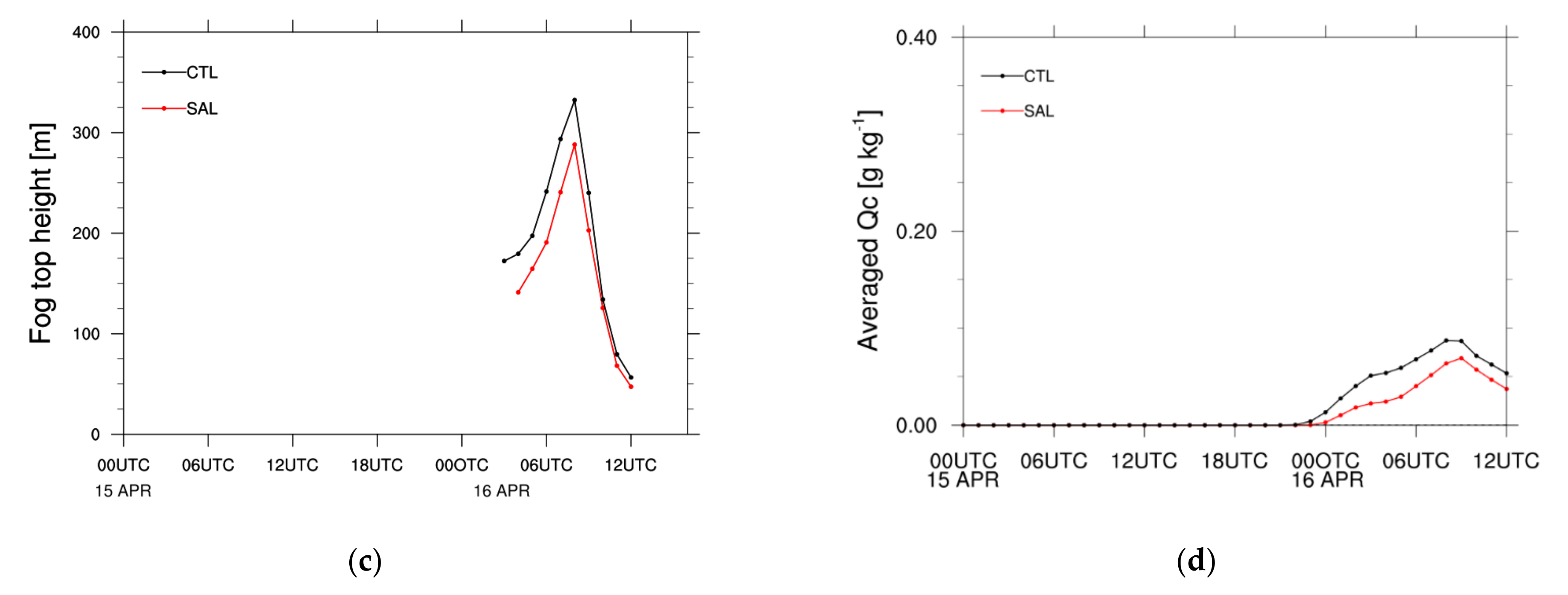
3.2.5. Sensitivity Test to Sea Surface Salinity

In most models of numerical weather prediction, the ocean surface is assumed to be saturated with pure water in the bulk formula for estimating surface turbulent fluxes, such as SHF and LHF. However, previous research has emphasized the importance of sea surface salinity in numerical weather forecasts. Studies have reported that the resulting dryness within the MABL due to the sea surface salinity improves the simulated convective precipitation [35]. Therefore, the impact of sea surface salinity on the evolution of the fog is discussed in this section.
According to Raoult’s Law, the saturated vapor pressure with respect to seawater is lower than that with respect to pure water. It was suggested in a previous study that the saturated vapor pressure with respect to seawater in terms of the saturated vapor pressure with respect to pure water is expressed as [35]:
e s , s w = e s , p w 1 + 0.57357 S / 1000 S
where e s , s w and e s , p w are the saturated vapor pressures for seawater and pure water (hPa), respectively, and S is the sea surface salinity (psu). To investigate the impact of sea surface salinity on the evolution of the sea fog, this revised saturated vapor pressure was used in an additional experiment. The initial condition for sea surface salinity was taken from salinity values of the Argo gridded dataset (http://apdrc.soest.hawaii.edu/projects/Argo/data/gridded/On_standard_levels/index-1.html; accessed on 1 August 2020), which was produced by the International Pacific Research Center (IPRC). Most Argo data do not have a salinity value on the surface. Accordingly, the first-level depth (5 m) was used as the sea surface salinity because it could be assumed that the ocean mixed layer has homogenous salinity. Hereafter, the previous experiment is referred to as CTL and this experiment is referred to as SAL.
It was found that incorporating the salinity effect in the numerical simulation decreased LHF due to the decrease in the saturated vapor pressure and specific humidity over the ocean surface. A decrease in LHF implies less transport of moisture from the ocean to the atmosphere during a fog event. Meanwhile, it was observed that the salinity effect had little influence on the SHF. Figure 15 represents the evolution of vertical profiles of the Qc simulated from SAL. SAL tends to simulate weaker and shallower fog, compared to CTL, due to a smaller amount of Qc during the fog event.
The rapid vertical jump of the fog also appears in SAL, similar to that in CTL. SAL simulated a synoptic-scale condition that was similar to that in CTL. Cold advection caused by the northerly wind due to the change in the large-scale flow was also shown, thus, an increase in thermal instability was also observed (not shown). According to the results, it was established that the rapid growth of sea fog was predominantly induced by cold advection.
The difference in sea fog between CTL and SAL is shown in the comparison of the top heights and amounts of the sea fog (Figure 16). The top heights and amounts of the sea fog were estimated as the maximum height with Qc of 0.01 g kg−1 and Qc averaged for the levels lower than a height of 500 m. In SAL, the top height was lower, and the formation and dissipation also occurred 1 h later and earlier, respectively, compared to that in CTL. In addition to the top height of the fog, the smaller amount of Qc was also simulated in SAL, which can influence higher visibility. It was caused by a decrease in LHF and weakening self-moistening locally, which resulted in suppressing the condensation in the microphysics process under the drier conditions. This suggests that considering sea surface salinity in the short-term weather prediction model predominantly has an impact on the formation, evolution, and dissipation processes of the sea fog.

4. Discussion

This case study improves our understanding of all processes related to the formation, evolution, and dissipation of each sea fog type. In particular, this study investigated the mechanism of the mixed type of cold-sea and warm-sea fog. Detailed findings from the simulated fog event helped in understanding the key features and characteristics of different types of sea fog, which can be eventually useful for providing better guidance for fog detection using remote sensing (e.g., satellite) and/or in situ observations. Considering that the accuracy of satellite (or remote sensing)-based fog detection differs depending on the fog type, understanding the key ingredients in different fog types and finding new fog types (i.e., the mixed type in this study) are fundamental and essential to improve the remote sensing-based fog detection algorithms.
To achieve this goal, further studies are still needed to verify the simulated fog. First, it is clear that a rapid upward diffusion is strongly related to turbulence, and can be highly dependent on the PBL scheme. Thus, overestimation of the height of the sea fog top should be confirmed by investigating the sensitivity of its vertical diffusion in various PBL schemes (e.g., local schemes vs. nonlocal schemes). Second, the maximum value of Qc is larger in the simulation, compared with one in the previous studies (about 0.6 g/kg) [36]. It can be understood that WRF simulation is likely to overestimate the amount of Qc, thus it can be more difficult to dissipate in the simulation than the real situation. Third, although the existence and visibility of sea fog can be validated using satellite and in situ observed data, the vertical structure can be also validated using information estimated from satellite sensors. However, this approach has limitations: information from satellites is not available under cloudy conditions (e.g., satellites with infrared sensors), and polar orbiting satellites do not provide continuous information for the diurnal evolution of the sea fog. Thus, it is difficult to confirm the overestimation of sea fog in the simulation. Therefore, intense observational sites (i.e., super sites) and/or field campaigns focusing on various fog events under different synoptic-scale conditions are needed to understand the more detailed generation mechanisms of fog evolution by measuring the height of the fog top and turbulent fluxes directly.

5. Conclusions

To understand the mechanisms in the formation, evolution, and dissipation stages of sea fog, particularly the mixed type of cold-sea and warm-sea fog, a sea fog event over the eastern Yellow Sea on 15–16 April 2012 was investigated using a high-resolution numerical simulation of the WRF model after it was verified by satellite data and in situ data. The verification showed that the simulation had good agreement with the observations in the formation, evolution, and dissipation phases of the sea fog. The mechanisms of a mixed type of cold-sea and warm-sea fog were as follows:
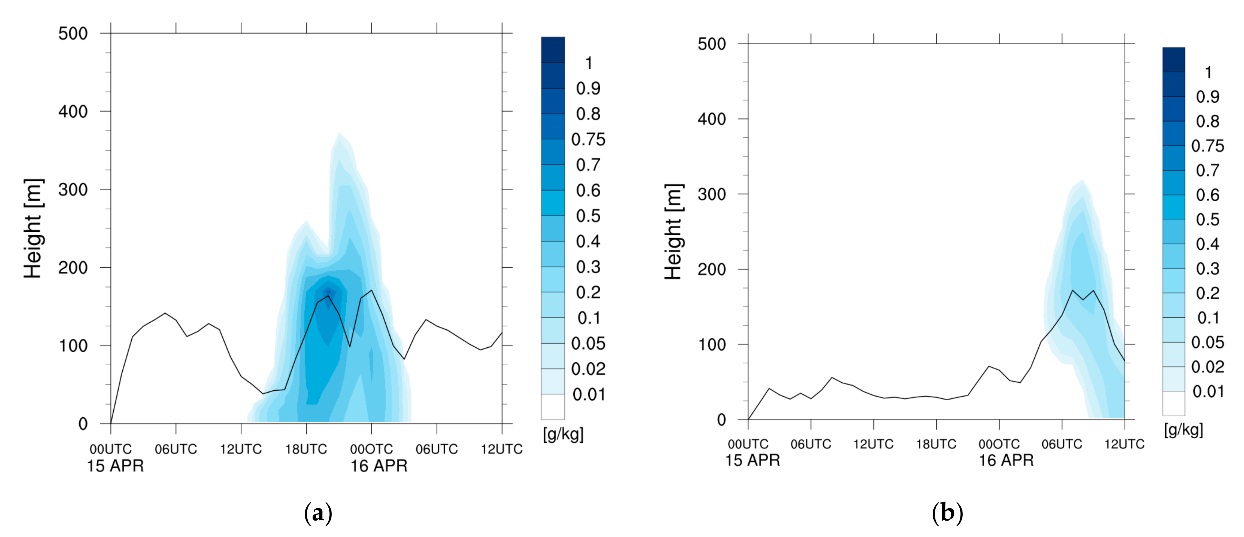
  • Initially, moist advection and cooling at z1 by downward SHF and LRC triggered the formation of the sea fog near the surface, and this fog was a conventional type of advection fog.
  • The intensified cooling near the surface transformed the SHF from downward to upward and increased LHF, which enhanced turbulent mixing and also moistened the lower atmosphere locally without moist advection. In this case, a transition from cold-sea fog to warm-sea fog was found at the evolution stage via observation of the changes to the conditions favorable for warm-sea fog.
  • Enhanced turbulent mixing and moistening due to surface turbulent fluxes increased the depth of the sea fog and the MABL height, even at night. This suggests that turbulence has a different impact on the growth of the MABL in accordance with the cold-sea and the warm-sea fogs.
  • Cold advection in this event due to the change to a northerly synoptic wind along with the maximum LRC at the top of condensed layer led to strong upward diffusion of the fog. It was proven using TKE budget analysis that cold advection contributed to a rapid increase in the MABL resulting from a strong positive buoyant forcing due to an increase in thermal instability.
  • Meanwhile, after sunrise, SW warming in the condensed layer offsetting the LRC reduced the MABL height, which resulted in trapping the fog within the low atmosphere. In addition, dry advection contributed to the dissipation of the fog due to the increase in evaporation.
  • Furthermore, the advection of Qc played an important role in controlling the local amount of fog, in which RH was not sufficient for saturation to cause fog.
  • Finally, an additional sensitivity test considering sea surface salinity showed weaker and shallower sea fog than the control run due to a decrease in both LHF and self-moistening locally. Thus, it can be expected that the overestimation of its depth was alleviated.
It is worth noting that this study focused on detailed mechanisms for the transition of a cold-sea fog to a warm-sea fog that have been rarely studied in previous studies. Besides, this study reveals that cold advection may have an effect on the rapid increase in MABL and fog depth. This study suggests that the turbulence is associated with all phases (formation, growth, and dissipation) of the sea fog, although numerous studies on the mechanism of sea fog have focused on the radiation and microphysics processes. This also reveals that turbulence has a different impact on the growth of the MABL in accordance with the cold-sea and warm-sea fog. This will provide more useful information for improving both forecasts and detections of fog using numerical prediction models and remote sensing/in situ observation, which helps to reduce possible accidents and damage in transportation operations under low visibility conditions due to fogs.

Author Contributions

E.L. and J.-H.K. performed the analysis and wrote the main body of the manuscript. E.L. ran the model, and takes responsibility for data curation and quality control. J.-H.K. conceptualized the idea of the project, and supervised the computer and funding resources. K.-Y.H. provided scientific advice to support the project. Y.-K.C. took a responsibility for the project administration, provided invaluable scientific suggestions and comments. E.L. wrote the original manuscript, and J.-H.K. reviewed and edited the original manuscript. All authors contributed critical feedback to this paper. All authors have read and agreed to the published version of the manuscript.

Funding

This work was funded by the Korea Meteorological Administration Research and Development Program under Grant KMI2020-01910, and was also supported by the Basic Science Research Program through the National Research Foundation of Korea (NRF) funded by the Ministry of Education (NRF-2019R1I1A2A01060035).

Data Availability Statement

The data presented in this study are available on request from the corresponding author.

Acknowledgments

We thank three anonymous reviewers and editors for their invaluable comments and suggestions on the original manuscript. We thank Kook-Jin Kim at the Underwater Survey Technology 21 (UST21) company and Young-Taek Kim at the Korea Hydrographic and Oceanographic Agency (KHOA) for their supports for the project. This work was also supported by project of “Machine Learning-Based Prediction and Accuracy Improvement of Sea Fog Dissipation” funded by the KHOA.

Conflicts of Interest

The authors declare no conflict of interest.

References

  1. Gultepe, I.; Milbrandt, J.A.; Zhou, B. Marine fog: A review on microphysics and visibility prediction. In Marine Fog: Challenges and Advancements in Observations, Modeling, and Forecasting; Koracin, D., Dorman, C., Eds.; Springer International Publishing: Berlin/Heidelberg, Germany, 2017; pp. 345–394. [Google Scholar]
  2. Garmon, J.F.; Darbe, D.L.; Croft, P.J. Forecasting significant fog on the Alabama coast: Impact climatology and forecast checklist development. NWS Tech. Memo. NWS SR 1996, 176, 16. [Google Scholar]
  3. Khvorostyanov, V.I.; Curry, J.A.; Gultepe, I.; Strawbridge, K. A springtime cloud over the Beaufort Sea Polynya: 3D simulation with explicit microphysics and comparison with observations. J. Geophy. Res. Atmos. 2003, 108, 4296. [Google Scholar] [CrossRef] [Green Version]
  4. Koračin, D.; Dorman, C.E.; Lewis, J.M.; Hudson, J.G.; Wilcox, E.M.; Torregrosa, A. Marine fog: A review. Atmos. Res. 2014, 143, 142–175. [Google Scholar] [CrossRef]
  5. Yang, L.; Liu, J.-W.; Ren, Z.-P.; Xie, S.-P.; Zhang, S.-P.; Gao, S.-H. Atmospheric conditions for advection-radiation fog over the western Yellow Sea. J. Geophys. Res. Atmos. 2018, 123, 5455–5468. [Google Scholar] [CrossRef]
  6. Kim, C.-K.; Yum, S.-S. Local meteorological and synoptic characteristics of fogs formed over Incheon international airport in the west coast of Korea. Adv. Atmos. Sci. 2010, 27, 761–776. [Google Scholar] [CrossRef]
  7. Cho, Y.-K.; Kim, M.-O.; Kim, B.-C. Sea fog around the Korean Peninsula. J. Appl. Meteorol. 2000, 39, 2473–2479. [Google Scholar] [CrossRef]
  8. Zhang, S.-P.; Xie, S.-P.; Liu, Q.-Y.; Yang, Y.-Q.; Wang, X.-G.; Ren, Z.-P. Seasonal variations of Yellow Sea fog: Observations and mechanisms. J. Clim. 2009, 22, 6758–6772. [Google Scholar] [CrossRef]
  9. Gultepe, I.; Isaac, G.; Williams, A.; Marcotte, D.; Strawbridge, K. Turbulent heat fluxes over leads and polynyas and their effect on Arctic clouds during FIRE-ACE: Aircraft observations for April 1998. Atmos. Ocean 2003, 41, 15–34. [Google Scholar] [CrossRef]
  10. Croft, P.J.; Darbe, D.L.; Garmon, J.F. Forecasting significant fog in southern Alabama. Natl. Weather Dig. 1995, 19, 10–16. [Google Scholar]
  11. Gultepe, I.; Pagowski, M.; Reid, J. A Satellite-Based Fog Detection Scheme Using Screen Air Temperature. Wea. Forecast. 2007, 22, 444–456. [Google Scholar] [CrossRef]
  12. Gultepe, I.; Muller, M.D.; Boybeyi, Z. A New Visibility Parameterization for Warm-Fog Applications in Numerical Weather Prediction Models. J. Appl. Meteorol. Climatol. 2006, 45, 1469–1480. [Google Scholar] [CrossRef]
  13. Gultepe, I.; Isaac, G.A. Effects of air mass origin on Arctic cloud microphysical parameters for April 1998 during FIRE. ACE. J. Geophys. Res. 2002, 107, SHE-4-1–SHE-4-12. [Google Scholar]
  14. Gultepe, I.; Isaac, G.A.; Strawbridge, K. Variability of cloud microphysical and optical parameters obtained from aircraft and satellite remote sensing during RACE. Inter. J. Climatol. 2001, 21, 507–525. [Google Scholar] [CrossRef]
  15. Kim, C.-K.; Yum, S.-S. A numerical study of sea-fog formation over cold sea surface using a one-dimensional turbulence model coupled with the Weather Research and Forecasting Model. Boundary Layer Meteorol. 2012, 143, 481–505. [Google Scholar] [CrossRef]
  16. Skamarock, W.C.; Klemp, J.B.; Dudhia, J.; Gill, D.O.; Liu, Z.; Berner, J.; Wang, W.; Powers, J.G.; Duda, M.G.; Barker, D.M.; et al. A Description of the Advanced Research WRF Version 4; NCAR Tech. note NCAR/TN556+STR; NCAR Library: Boulder, CO, USA, 2019; p. 145. [Google Scholar]
  17. Hong, S.-Y.; Noh, Y.; Dudhia, J. A new vertical diffusion package with an explicit treatment of entrainment processes. Mon. Wea. Rev. 2006, 134, 2318–2341. [Google Scholar] [CrossRef] [Green Version]
  18. Lim, K.-S.S.; Hong, S.-Y. Development of an effective doublemoment cloud microphysics scheme with prognostic cloud condensation nuclei (CCN) for weather and climate models. Mon. Wea. Rev. 2010, 138, 1587–1612. [Google Scholar] [CrossRef] [Green Version]
  19. Mlawer, E.J.; Taubman, S.J.; Brown, P.D.; Iacono, M.J.; Clough, S.A. Radiative transfer for inhomogeneous atmospheres: RRTM, a validated correlated-k model for the longwave. J. Geophys. Res. 1997, 102, 16663–16682. [Google Scholar] [CrossRef] [Green Version]
  20. Chen, F.; Dudhia, J. Coupling an advanced land surface hydrology model with the Penn State–NCAR MM5 modeling system. Part I: Model implementation and sensitivity. Mon. Wea. Rev. 2001, 129, 569–585. [Google Scholar] [CrossRef] [Green Version]
  21. Ek, M.B.; Mitchell, K.E.; Lin, Y.; Rogers, E.; Grunmann, P.; Koren, V.; Gayno, G.; Tarpley, J.D. Implementation of Noah land surface model advances in the National Centers for Environmental Prediction operational mesoscale Eta model. J. Geophys. Res. 2003, 108, 8851. [Google Scholar] [CrossRef]
  22. Tewari, M.; Chen, F.; Wang, W.; Dudhia, J.; LeMone, M.A.; Mitchell, K.; Ek, M.; Gayno, G.; Wegiel, J.; Cuenca, R.H. Implementation and verification of the unified NOAH land surface model in the WRF model. In Proceedings of the 20th Conference on Weather Analysis and Forecasting/16th Conference on Numerical Weather Prediction, USA, 1 January 2004; pp. 11–15. [Google Scholar]
  23. Jiménez, P.A.; Dudhia, J.; Gonzále-Rouco, J.F.; Navarro, J.; Montávez, J.P.; García-Bustamante, E. A revised scheme for the WRF surface layer formulation. Mon. Wea. Rev. 2012, 140, 898–918. [Google Scholar] [CrossRef] [Green Version]
  24. Kain, J.S.; Fritsch, J.M. Convective parameterization for mesoscale models: The Kain-Fritsch scheme. In The Representation of Cumulus Convection in Numerical Models; Emanuel, K.A., Raymond, D.J., Eds.; Springer International Publishing: Berlin/Heidelberg, Germany, 1993; pp. 165–170. [Google Scholar]
  25. Underwood, S.J.; Ellrod, G.P.; Kuhnert, A.L. A multiple-case analysis of nocturnal radiation-fog development in the central valley of California utilizing the GOES nighttime fog product. J. Appl. Meteorol. 2004, 43, 297–311. [Google Scholar] [CrossRef]
  26. Ellrod, G.P. Advances in the detection and analysis of fog at night using GOES multispectral infrared imagery. Wea. Forecast. 1995, 10, 606–619. [Google Scholar] [CrossRef] [Green Version]
  27. Yamanouchi, T.; Suzuki, K.; Kawaguchi, S. Detection of clouds in Antarctica from infrared multispectral data of AVHRR. J. Meteorol. Soc. Jpn. 1987, 65, 949–962. [Google Scholar] [CrossRef] [Green Version]
  28. Steeneveld, G.J.; Tolk, L.F.; Moene, A.F.; Hartogensis, O.K.; Peters, W.; Holtslag, A.A.M. Confronting the WRF and RAMS mesoscale models with innovative observations in the Netherlands: Evaluating the boundary layer heat budget. J. Geophys. Res. 2011, 116, D23114. [Google Scholar] [CrossRef]
  29. Lin, C.; Zhang, Z.; Pu, Z. Numerical simulations of an advection fog event over Shanghai Pudong International Airport with the WRF model. J Meteorol Res. 2017, 31, 874–889. [Google Scholar] [CrossRef]
  30. Carlos, R.-C.; Carlos, Y.; Gert-Jan, S.; Gema, M.; Jon, A.A.; Mariano, S.; Gregorio, M. Radiation and cloud-base lowering fog events: Observational analysis and evaluation of WRF and HARMONIE. Atmos. Res. 2019, 229, 190–207. [Google Scholar] [CrossRef]
  31. Lee, H.-Y.; Chang, E.-C. Impact of land-sea thermal contrast on the inland penetration of sea fog over the coastal area around the Korean Peninsula. J. Geophys. Res. Atmos. 2018, 123, 6487–6504. [Google Scholar] [CrossRef]
  32. Lenschow, D.H. Model of the height variation of the turbulent kinetic energy budget in the unstable planetary boundary layer. J. Atmos. Sci. 1974, 31, 465–474. [Google Scholar] [CrossRef] [Green Version]
  33. Shin, H.H.; Hong, S.-Y.; Noh, Y.; Dudhia, J. Derivation of Turbulent Kinetic Energy from a First-Order Nonlocal Planetary Boundary Layer Parameterization. J. Atmos. Sci. 2013, 70, 1795–1805. [Google Scholar] [CrossRef] [Green Version]
  34. Kim, C.-K.; Yum, S.-S. Marine Boundary Layer Structure for the Sea Fog Formation off the West Coast of the Korean Peninsula. Pure Appl. Geophys. 2012, 169, 1121–1135. [Google Scholar] [CrossRef]
  35. Lee, E.; Hong, S.-Y. Impact of the sea surface salinity on simulated precipitation in a global numerical weather prediction model. J. Geophys. Res. Atmos. 2019, 124, 719–730. [Google Scholar] [CrossRef]
  36. Gultepe, I.; Pearson, G.; Milbrandt, J.A.; Hansen, B.; Platnick, S.; Taylor, P.; Gordon, M.; Oakley, J.P.; Cober, S.G. The Fog Remote Sensing and Modeling Field Project. Bull. Am. Meteor. Soc. 2009, 90, 341–360. [Google Scholar] [CrossRef]
Figure 1. Geographical map of the eastern Yellow Sea and its neighboring regions with four model domains.
Remotesensing 13 01480 g001
Figure 2. Synoptic weather charts for sea level pressure (SLP) (a,c,e) generated by the Korea Meteorological Administration (KMA), and (b,d,f) simulated for domain 1; (a,b) 1200 UTC on 15 April 2012, (c,d) 0000 UTC on 16 April in 2012, and (e,f) 1200 UTC on 16 April in 2012. Wet areas shaded with green dots are defined as T-Td < 3 K and the arrows indicates a 10 m wind (m s−1). (g) Skew T-Log P diagram in Baekneyong island (124.38°E, 37.55°N) at 1200 UTC on 15 April 2012 (blue) and at 0000 UTC on 16 April 2012.
Remotesensing 13 01480 g002aRemotesensing 13 01480 g002bRemotesensing 13 01480 g002c
Figure 3. (a,c,e) Near-infrared images from the Communication, Ocean and Meteorological Satellite (COMS) operated by the KMA and (b,d,f) distributions of simulated Qc (g kg−1) averaged for the levels lower than a 100 m height for domain 3; (a,b) 1200 UTC on 15 April, (c,d) 0000 UTC on 16 April, and (e,f) 1200 UTC on 16 April in 2012. Fog areas are denoted by yellow (potential) and orange (detected) shading in the near-infrared images. The cross signs indicate the oceans near Baekneyong island (124.38°E, 37.55°N) and Heuksan island (125.42°E, 34.67°N) stations, that provide data from sounding observations.
Remotesensing 13 01480 g003aRemotesensing 13 01480 g003b
Figure 4. Evolution of vertical profiles of the (a,b) relative humidity (RH; %) with the marine atmospheric boundary layer (MABL) height (thick solid line, m) and (c,d) Qc (g kg−1) with the estimated height of the fog top from the MTSAT-2 satellite data (dot, m) in domain 4, averaged over the nearby oceans; (a,c) Baeknyeong island (hereafter region A) and (b,d) Heuksan island (hereafter region B).
Remotesensing 13 01480 g004
Figure 5. Comparison of observed (red dots) and simulated (blue solid lines) vertical profiles of the (a,b) temperature (°C) and (c,d) specific humidity (g kg−1) during the fog event (a,c) at the Baeknyeong island station at 0000 UTC 16 April 2012 and (b,d) at the Heuksan island station at 1200 UTC 16 April 2012.
Remotesensing 13 01480 g005
Figure 6. Time series of the (a) surface turbulent fluxes (blue: turbulent latent heat flux; LHF, red: turbulent sensible heat flux; SHF) and (b) MABL height in region A during the formation and evolution stages.
Remotesensing 13 01480 g006
Figure 7. Time series of the hourly accumulated tendencies of the (a) temperature (°C h−1), (b) Qv (g kg−1 h−1), and (c) Qc (g kg−1 h−1) at z1 in region A during the formation and evolution stages. PBL, RAD, ADV, and MPS, indicate planetary boundary layer, radiation, advection, and microphysics processes, respectively, and TOT represents the summation of their tendencies.
Remotesensing 13 01480 g007aRemotesensing 13 01480 g007b
Figure 8. Vertical profiles of the hourly accumulated tendencies of (ac) temperature (°C h−1), (df) Qv (g kg−1 h−1), and (gi) Qc (g kg−1 h−1) in region A; (a,d,g) 1100 UTC (before the onset of the fog), (b,e,h) 1200 UTC (after the onset of the fog), and (c,f,i) 1700 UTC (at the vertical jump of the fog) on 15 April in 2012. SW, LW indicate shortwave and longwave radiative fluxes, respectively.
Remotesensing 13 01480 g008aRemotesensing 13 01480 g008b
Figure 9. Sea surface temperature (Ts) and surface air temperature (Ta) observed from AWS and buoy data at Deokjeok island.
Remotesensing 13 01480 g009
Figure 10. Turbulent kinetic energy (TKE) budget from the simulation, normalized by surface buoyancy production: buoyancy production (BP, red line) and shear production (SP, blue line).
Remotesensing 13 01480 g010
Figure 11. Vertical profiles of the hourly accumulated tendencies of (a,b) temperature (°C h−1), (c,d) Qv (g kg−1 h−1), and (e,f) Qc (g kg−1 h−1) in region A: (a) 0000 UTC (before the dissipation of the fog), and (b) 0300 UTC (after the dissipation of the fog) on 16 April in 2012.
Remotesensing 13 01480 g011
Figure 12. Time series of the (a) hourly accumulated tendency of Qc (g kg−1 h−1) averaged for levels below a height of 300 m and (b) MABL height in region B during the fog event.
Remotesensing 13 01480 g012
Figure 13. Vertical cross section of Qc (shading) and wind (vector) along the line passing by the two regions A and B at (a) 0000 UTC, (b) 0200 UTC, and (c) 0400 UTC on 16 April.
Remotesensing 13 01480 g013
Figure 14. Vertical profiles of the hourly accumulated tendency of Qc (g kg−1 h−1) in region B at 0400 UTC on 16 April in 2012.
Remotesensing 13 01480 g014
Figure 15. Evolution of vertical profiles of the Qc (g kg−1) in (a) region A and (b) region B simulated from SAL.
Remotesensing 13 01480 g015
Figure 16. Time series of the estimated height of the (a,c) fog top (m) and (b,d) Qc averaged for the levels lower than a height of 500 m (g kg−1) from CTL (black line) and SAL (red line): (a,b) region A and (c,d) region B.
Remotesensing 13 01480 g016aRemotesensing 13 01480 g016b
Table 1. Experimental settings of the Weather Research and Forecasting (WRF) model.
ModelWRF v4.2
Nesting methodOne-way data
Horizontal resolution4 domains (27, 9, 3, 1 km)
Vertical levels
(eta levels)
51 levels
Time step (s)180 s (D1), 60 s (D2), 20 s (D3), 6.6 s (D4)
Initial and boundary
conditions
Atmos: NCEP FNL (1° × 1°),
SST: daily OISST (0.25° × 0.25°)
Table 2. Configuration of the physics package.
ProcessScheme
RadiationRRTM (SW), Duhia (LW)
MicrophysicsWRF Double-Moment 6-class (WDM6)
Deep cumulusKain–Fritsch cumulus parameterization scheme
Planetary boundary layerYonsei University (YSU)
Land surfaceUnified Noah land surface model
Surface layerRevised MM5 Monin–Obukhov surface layer scheme
Publisher’s Note: MDPI stays neutral with regard to jurisdictional claims in published maps and institutional affiliations.

