Article

Effective Selection of Variable Point Neighbourhood for Feature Point Extraction from Aerial Building Point Cloud Data

School of Information and Communication Technology, Griffith University, Nathan, QLD 4111, Australia
*
Author to whom correspondence should be addressed.
Submission received: 18 March 2021 / Revised: 9 April 2021 / Accepted: 12 April 2021 / Published: 15 April 2021
(This article belongs to the Special Issue 3D Urban Modeling by Fusion of Lidar Point Clouds and Optical Imagery)

Abstract

:
Existing approaches that extract buildings from point cloud data do not select the appropriate neighbourhood for estimation of normals on individual points. However, the success of these approaches depends on correct estimation of the normal vector. In most cases, a fixed neighbourhood is selected without considering the geometric structure of the object and the distribution of the input point cloud. Thus, considering the object structure and the heterogeneous distribution of the point cloud, this paper proposes a new effective approach for selecting a minimal neighbourhood, which can vary for each input point. For each point, a minimal number of neighbouring points are iteratively selected. At each iteration, based on the calculated standard deviation from a fitted 3D line to the selected points, a decision is made adaptively about the neighbourhood. The selected minimal neighbouring points make the calculation of the normal vector accurate. The direction of the normal vector is then used to calculate the inside fold feature points. In addition, the Euclidean distance from a point to the calculated mean of its neighbouring points is used to make a decision about the boundary point. In the context of the accuracy evaluation, the experimental results confirm the competitive performance of the proposed approach of neighbourhood selection over the state-of-the-art methods. Based on our generated ground truth data, the proposed fold and boundary point extraction techniques show more than 90% F1-scores.

Graphical Abstract

1. Introduction

Estimation of the feature points and lines is a fundamental problem in the field of image and shape analysis as this estimation facilitates better understanding of an object in a variety of areas, e.g., data registration [1], data simplification [2], road extraction [3], and building reconstruction [4]. Specifically, the area of 3D building reconstruction has a broad range of applications, such as building type classification, urban planning, solar potential estimation, change detection, forest management, and virtual tours [5,6,7,8,9,10]. Due to the availability of 3D point cloud data, from both airborne and ground-based mobile laser scanning systems, the extraction of 3D feature points and lines from point cloud data has become an attractive research topic to describe an object shape more accurately.
The airborne Light Detection and Ranging (LiDAR) data from a geographic location is a set of unordered points. It mainly consists of the parameters from three independent dimensions with X, Y, and Z coordinates along with other retro-reflective properties generally in the form of intensities. These parameters and properties together can describe the topographic profile of the Earth’s surface and object at that location [11]. Therefore, LiDAR data provide more accurate geometric information than the 2D image and are used as the main input data for automatic building reconstruction [12,13]. The reconstruction approaches from LiDAR data can be broadly categorised into two: model-driven and data-driven [7]. The first approach finds the most similar models previously stored in the database to the input data, whereas the second approach tries to generate any building model from the provided 3D data. The data-driven approach mainly finds different features, e.g., planer patches, lines, curves, angles, and corners, which represent the major components of a building structure, from the input building point cloud. By correctly grouping those features and geometric topologies, the models of the buildings are generated. To reconstruct the buildings, individual planar patches are firstly identified using one or more of the different segmentation algorithms such as region growing [14]. After that, the neighbouring segments are identified and the relationship among the patches are established based on different features such as co-planarity, intersection lines, corners, and edges [15]. Therefore, feature point extraction to construct feature lines and edges to establish a relationship among the planar patches in the 3D point cloud data is the main challenge for building reconstruction techniques in the data-driven approach. While the model driven approach is limited to the models in the library, the data driven approach works in general for any building roof shape.
Although various definitions of the 3D object edges can be found in the literature [16,17,18], in the area of building reconstruction, many of the authors categorised the 3D edges into the boundary and fold edges [16,19]. Roof contours and facade outlines are referred to as boundary edges [19], and fold edges or sharp feature lines are defined as the intersecting edges of two or more planes [10,20]. Ni et al. [16] considered that boundary elements have an abrupt angular gap in the shape formed by their neighbouring points and that the points in the fold edges have an abrupt directionality change between the directions in adjacent surfaces. Existing research on edge extraction in point clouds mostly considers either statistical and geometrical methods or the directionality and geometric changes [21]. To measure the directionality and the geometric changes, the estimation of normal and curvature for each 3D point in the data is an important factor and should be calculated accurately [22]. However, estimation of the normal vector along a building edge highly depends on the neighbourhood employed for each point [21,23], and the inharmonious nature of LiDAR point cloud makes the calculation of that neighbourhood complex and challenging [22,24]. Moreover, noise associated in the oblique point cloud data can create serious problems for calculating accurate normals in the context of affective and automatic building plane reconstruction [25].
Consequently, the k-neighbourhood (also, known as k-nearest neighbours or k-NN) and r-neighbourhood [26] are two traditional approaches in selecting neighbours of a given point P i . The former selects k number of nearest points from P i , and the latter contains all points for which the distance to P i is less than or equal to r. Selecting the value for k or r is challenging as the local geometry of the object is unknown [17]. A higher value of k or r may reduce the impact of noise on the estimated normal but information from several classes or planes can be mixed up in one neighbourhood, thus producing a wrong estimation [27]. In contrast, a lower value can prevent the capture of enough shape information [27]. Figure 1 shows that, while a small neighbourhood for P 3 may offer an unstable normal estimation due to local variations (e.g., corrugations on a metallic roof), a large neighbourhood for P 2 can skip the local variations and thus offers a better estimation. However, large neighbourhoods for P 1 and P 4 attract points from other planes and objects. Therefore, a wrong selection of neighbourhoods can result in a seriously faulty normal estimation. Nonetheless, the aircraft that holds the LiDAR system scans the studied area in a specific direction; thus, specific scanlines can be observed over the objects in the area. Figure 1 demonstrates the scanline direction (red arrows) of LiDAR points over a building roof.
Considering the LiDAR point density in addition to the heterogeneous point distribution, this paper proposes an effective neighbourhood selection method that is free from selecting any fixed parameter such as k or r. The proposed method finds the best fit 3D lines first and, then, considers the standard deviation of the fitted points. Based on the point density of the input data and the distance pattern of scanlines, it selects the minimal number of neighbours automatically for each point in the point cloud. The direction of the normal is then calculated for each point to extract the fold feature points of the roof. The terms “fold edge point”, “fold feature point”, or “fold point” are used alternatively in this paper to indicate the same thing. Based on the distance from the mean value of the selected minimal neighbours, a decision can be made easily about whether a point is a boundary point.
The particular contributions of this paper are as follows:
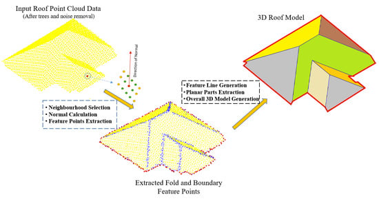
  • In the context of calculating an accurate normal, a new robust method is proposed for automatic selection of neighbouring points of each point in a LiDAR point cloud data. This proposed method can select the optimal minimum number of neighbouring points and, thus, can solve the existing problems of accurate normal calculation of individual points.
  • Based on the calculated direction of the normal, we propose an effective method for finding the fold feature points. Maximum angle differences of the neighbouring normal vectors are clustered, and an experimentally selected threshold is adopted to decide fold edge points.
  • To find the boundaries of individual objects, a new method for boundary point detection is suggested. This method depends on the distance from a point to the calculated mean of its neighbouring points, selected by the proposed technique of automatic neighbouring point selection.
The rest of the paper is organised as follows. Section 2 presents a review of the existing techniques for neighbourhood selection, normal calculation, and feature point extraction along with their challenges. The proposed method of neighbourhood selection along with the fold and boundary feature point extraction methods are discussed in Section 3. Extensive experimentations are presented and discussed in Section 4. Finally, Section 5 exposes the conclusion.

2. Review

The main objective of our work is to extract the feature points from point cloud data based on the minimal number of neighbourhood for each point. Calculation of the normal vectors is an important geometric property to find the feature points. Thus, in this section, firstly, we discuss the state-of-the-art approaches of neighbourhood selection methods. Secondly, we discuss existing methods for calculating the normal of a point. Finally, we discuss the existing methods for feature point extraction techniques.

2.1. Neighbourhood Selection

Most of the existing feature point extraction techniques use the geometric properties (e.g., curvature, discontinuity, and angle) of a point based on its k or r neighbourhoods in the input point cloud data. The classical Principal Component Analysis (PCA) can estimate the important geometric features of a point by collecting its k number of neighbours [23]. The minimal value of k needs to be chosen manually, but in practice, a single global k is often not suitable for an entire point cloud, where different objects in different regions may have different geometric structures or point densities [17,23]. A large value of k over-smooths the sharp feature points, while a small neighbourhood is more sensitive to local variations and noise [28].
To avoid these issues, some authors proposed adaptive approaches instead of using the fixed minimal neighbourhood. For example, Elong et al. [29] used a curvature-based adaptive neighbourhood selection technique to classify point cloud data. Considering the calculated curvature value of each point, the author divided an input point cloud into scatter and regular regions. After that, they selected adaptive values of k and r for scatter and regular regions, 10 k 50 and 0.5 m r 2.5 m, respectively, within fixed intervals to reduce the computational complexities. Weinman et al. [30,31] used a Shannon entropy-based [32] neighbourhood selection method to select k closest neighbours within a fixed predefined interval, where 10 k 100 . For different values of k, they found different entropies for each point and finally chose the value k, which satisfied the minimum entropy. Wang et al. [23] proposed a self-attention-based normal estimation architecture, where they claimed that the network could select the minimal number of neighbouring points according to the local geometric properties that initially provided a large k number of neighbourhoods of a point. They applied a multi-head self-attention module that selects the neighbouring points softly according to the local geometric properties. However, this method worked at the expense of the high computational cost associated with the Convolutional Neural Network (CNN). Ben-Shabat et al. [28] used a point-wise multiscale 3D modified Fischer Vector (3DmFV) [33] representation to encode the local geometry (e.g., normal) of a point using a CNN. They found n subsets of points for each point in the original input point cloud. Each subset was referred to as a scale that contained a different number of points instead of fixed neighbours. The 3DmFV representation was then calculated for each scale. All 3DmFVs were provided as input to a CNN to find the normal of a point. Some authors used a multiscale neighbourhood selection approach for the classification of point clouds [27,34]. For example, Leichter et al. [27] introduced and applied a multiscale approach to recover the neighbourhood in an unstructured 3D point cloud. Both the k and r neighbourhoods were used at different scales with the aim to improve the classification accuracy. The major drawback of this approach is the high computational complexity. Besides this, these methods experience drawbacks from the so-called Hughes phenomenon [35], where the classification accuracy decreases for growing feature space dimensionality.

2.2. Normal Vector Calculation

The normal vectors of points in a point cloud are important geometric properties that have been widely used by many authors to find the fold and boundary points, and high-quality surfaces [17,21,24,36,37]. Although there are several methods for estimating normal vectors in a point cloud, they are mainly proposed for 3D geometric models that have less noise with high point densities and most of the models contain smooth surfaces. In the case of buildings in a typical urban environment, the situation is complex. LiDAR data often have low point density and nonuniform sampling rate and contain a lot of noise [25]. Therefore, the accurate calculation of normal vectors in this situation is challenging.
The literature on estimating normal vectors can be divided into two major approaches: combinatorial and numerical [37]. The combinatorial approach uses mainly Delaunay and Voronoi properties [38]. Although this approach can work in the presence of noise, in general, it becomes infeasible for large datasets. The numerical approach considers the neighbours of an interest point that may represent the surface locally, and the calculated normal of the surface is treated as the estimated normal of the point of interest. Finding a proper local neighbourhood and a best-fit plane for a point is the main issue in the numerical-based approach [30]. The PCA and its variations, for example, the Weighted PCA [39], Moving Least Square (MLS) Projection [40], Robust PCA (RPCA) [41], and Diagnostic-Robust PCA (DRPCA) [42], were used by different authors for calculating normal vectors by finding the best fitted plane. Considering specifically the oblique building point cloud data in urban environments, Zhu et al. [25] proposed an effective normal estimation method to handle the noise in building a point cloud through a local to global optimisation strategy. Instead of calculating the normal of individual points, they proceeded in a hierarchical fashion and merged similar points into supervoxels considering a planarity constraint to exclude outliers. Nurunnabi et al. [37] removed outliers using their proposed Maximum Consistency with Minimum Distance (MCMD) algorithms and then applied PCA to find normal vectors in a point cloud. Dey et al. [43] proposed an improved approach and solved the limitations of the MCMD to construct more accurate planes. Recently, Sanchez et al. [24] proposed a robust normal estimation technique through an iterative weighted PCA [39] and the robust statistical M-estimators [44]. In the weighted PCA, the neighbouring points are assigned different weights based on their distance to P i . Smaller distance points are assigned bigger weights in this approach. The M-estimators allow users to fit a model onto points by rejecting outliers. Chen et al. [17] proposed a method to extract the fold points based on the minimal number of clusters of the unit normal vectors using effective k-means clustering [45]. Using the k-neighbourhood, they calculated the normal vectors for each adjacent triangular plane constructed using any two points from the neighbours and the point itself. The directions of the unit normal vectors were calculated using a minimum spanning tree algorithm proposed by Guennebaud and Gross [46].
The major challenge in calculating the normal vectors for feature point extraction is selecting the minimal number of neighbouring points that directly influence the extraction process. The present literature mainly selects the minimal number of neighbours empirically, which is a manual process and does not consider the point cloud density and other factors. Besides this, the performance of these methods degrades in the presence of noise in the input point cloud data.

2.3. Feature Point Extraction

Existing 3D feature point extraction techniques can be broadly categorised into indirect (by converting 3D point clouds into images first) and direct (by extracting 3D edge points from the 3D-point cloud directly) approaches [11,47]. Indirect approaches take the advantages of traditional 2D edge point detection algorithms. The 3D point clouds are converted into 2D images first, and after that, the extracted lines or edge points from the 2D images are projected back to the 3D space [48,49,50]. Moghadam et al. [51] extracted feature points for the edge and boundary of an object to construct the 3D feature lines using corresponding 2D line segments of each part of the object. For each extracted 3D planar part, all of the 3D points were projected on a 2D plane [47]. Contours were extracted from the 2D segments and then projected back onto the 3D plane to obtain the 3D edge points and lines. These techniques fail to extract perfect 3D edges because of information loss during the 3D to 2D conversion and vice-versa and, thus, degrade the extraction accuracy [52].
The direct approach can also be subdivided by plane-based and direct point geometry-based approaches. Plane-based methods consider the intersections of two or more separate roof planes as the feature lines of a building. It is suitable because most buildings are a combination of different piecewise-planar roof planes [7,12,53]. Determination of planar surfaces is the main key point of this category. In this method, planar points are firstly separated from the non-planar feature points and then individual roof segments are extracted using different clustering and region growing approaches. Points of the intersecting roof plane segments are taken into consideration to form the feature lines [12]. For example, Ni et al. [16] proposed an easy-to-use 3D feature point extraction method namely Analyzing Geometric Properties of Neighbourhoods (AGPN). The authors defined the 3D edges as “3D discontinuities of the geometric properties in the underlying 3D-scene”. They combined the RANdom SAmple Consensus (RANSAC) [54] and angular gap metric [55] to extract edge feature points. This method can extract two kinds of feature points, i.e., boundary elements and fold edges, which actually include all types of edges in a point cloud data. Although the plane fitting-based methods show good extraction results for the cases of fold points, most of the time, they show less accuracy for boundary point extraction [17]. Besides this, the extraction of feature points using existing plane fitting-based methods does not perform well as it loses the sharp features when the intersecting planar patches are too small [17,47].
The direct point geometry-based approach can detect both boundary and inside sharp feature points based on different geometric properties such as azimuth angles [17], normal directions [21,56], and curvature variations [21]. For example, Chen et al. [17] considered the directions of the calculated normals and azimuth angles. For a fold point, they considered the direction of all the unit normal vectors of adjacent triangular planes and aggregated them into two different clusters. The directions of the unit vectors in each of the groups are very close to each other but far from each other. To detect the boundary points, they considered the azimuth angles. Statistical approaches, such as covariance and eigenvalues, and the combination of features derived from the PCA were also used in some cases [18,37]. In this paper, we focus on the direct point geometry-based approach to avoid the problems of image and plane fitting-based methods and concentrate on accurate normal estimation to extract the feature points.
Many authors used the following 3 × 3 covariance matrix Cov [ P , P ] of a point P to extract the point cloud feature points as a direct approach. The features are calculated based on different combinations of eigenvalues ( λ 1 λ 2 λ 3 ) and eigenvectors of Cov [ P , P ] [10,37,52,57]. Among different measures of feature point extraction from point-cloud data, the linearity and planarity measures are widely used [58]. These two properties of any point can be defined by Equations (1) and (2), respectively.
L = λ 1 λ 2 λ 1 .
P = λ 2 λ 3 λ 1 .
The main problem of feature point extraction based on the eigenvalues are the empirical determination of the thresholds and the selection of the neighbourhood [37].

3. Proposed Method

This paper suggests a new approach for selecting neighbouring points in the context of calculation of normal vectors and roof features. In this section, we present the proposed method for neighbourhood estimation followed by the proposed fold point extraction and boundary point detection.

3.1. Estimating Minimal Neighbourhood

The calculation of the normal vector is widely employed for extracting planes, boundaries, and edge features from LiDAR point cloud data. Most of the existing methods mainly considered high-density point cloud data with low noise, and their normal calculations are for 3D geometric models (e.g., statues and mechanical parts) having artificial or smooth surfaces. However, the nature of the aerial LiDAR data over an urban environment is different in the sense that they often contain noise, have low point density, and are heterogeneous in positions compared to the point cloud data over the 3D geometric models used by the existing methods.
The selection of the number of neighbouring points to calculate the normal vector is a great challenge. If we choose a high number of neighbours, then points from multiple planes can be aggregated (see Figure 1). If a low number of neighbouring points are chosen, they may be selected from a single straight scanline. In both cases, the calculation of the normal will be erroneous. While a small neighbourhood may be sensitive to the small variation in roof material, a large neighbourhood can attract outliers. In addition, the aerial LiDAR data come with a vertical accuracy of 15 to 30 cm. This accuracy issue can affect any size neighbourhood. Therefore, calculation of the normal using a dynamically selected minimal number of neighbourhood for each point is more suitable to circumvent these issues.
For each P i on a plane, the proposed neighbourhood selection method iteratively selects a larger neighbourhood and fits a 3D line L 3 to the neighbouring points. If all or most of these points are from the same scanline, then the line fitting error, for example, in terms of the standard deviation, will be low. In contrast, if they come from different scanlines, then the error will be high. A high error shows that the corresponding neighbourhood is large enough, it includes points from multiple scanlines and these points are minimal to form a normal of the plane. Figure 2 illustrates the flow diagram of the proposed neighbourhood estimation method that follows the steps below.
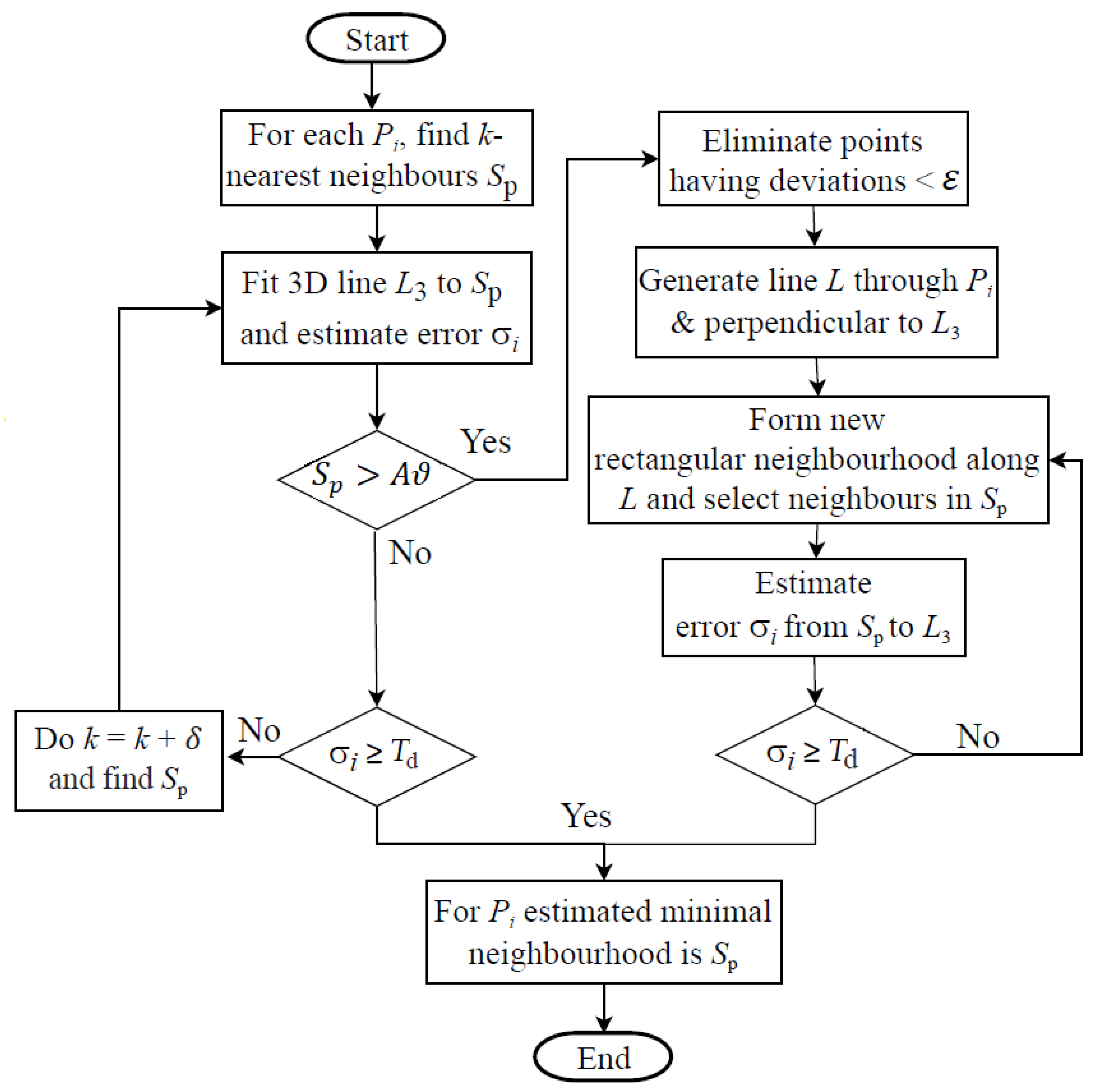
  • The proposed method first selects a minimal number of neighbouring points (say, k = 3 since a minimum of 3 points are necessary to calculate a plane normal) for P i using the k-NN algorithm. Let the set of neighbouring points be S p including the point P i .
  • A best fit 3D line L 3 is constructed using S p . The distance from each point of S p to L 3 is calculated.
  • The standard deviation σ i of the calculated distances is compared with a selected distance threshold T d . If σ i < T d , the value of k is increased (say, k = k + δ ) and the procedure is repeated with the updated S p . Ideally, δ = 1 is set to iteratively find a minimal value of k for P i . However, to avoid a large number of iterations, δ = 5 is selected and, once a minimal k is found, a smaller minimal k is obtained by testing its previous δ 1 values.
    T d is equal to the distance between two neighbouring points in the case of regular distribution of LiDAR points and can be calculated using Equation (3) according to Tarsha-Kurdi et al. [59], where ϑ represents the input point density. The mean area occupied by a single LiDAR point is in a square form, and the area of the square is equal to the inverse of the point density in a regular distributed point cloud data. The side length of the square represents the mean distance between two neighbouring points that satisfies Equation (3).
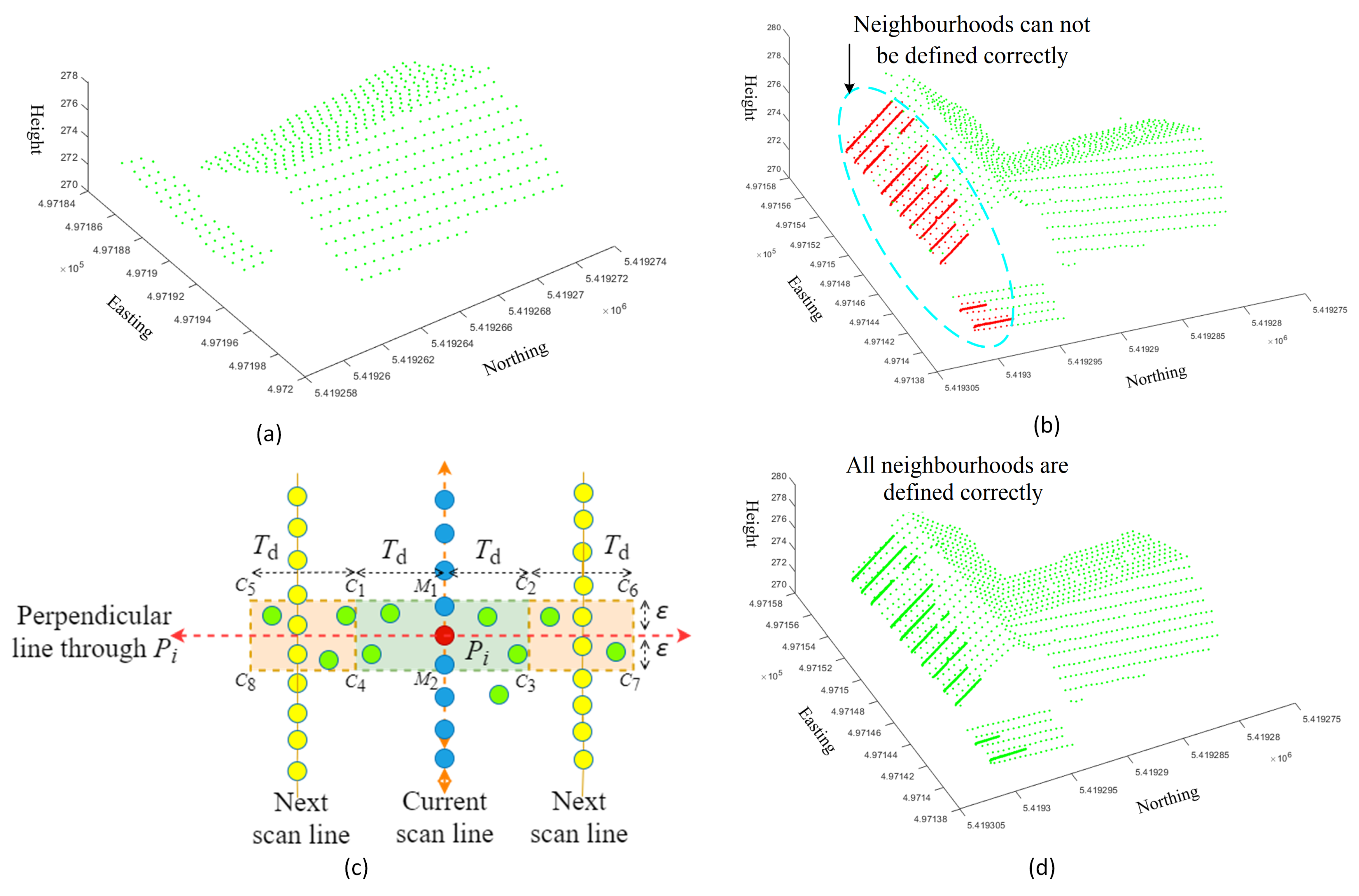
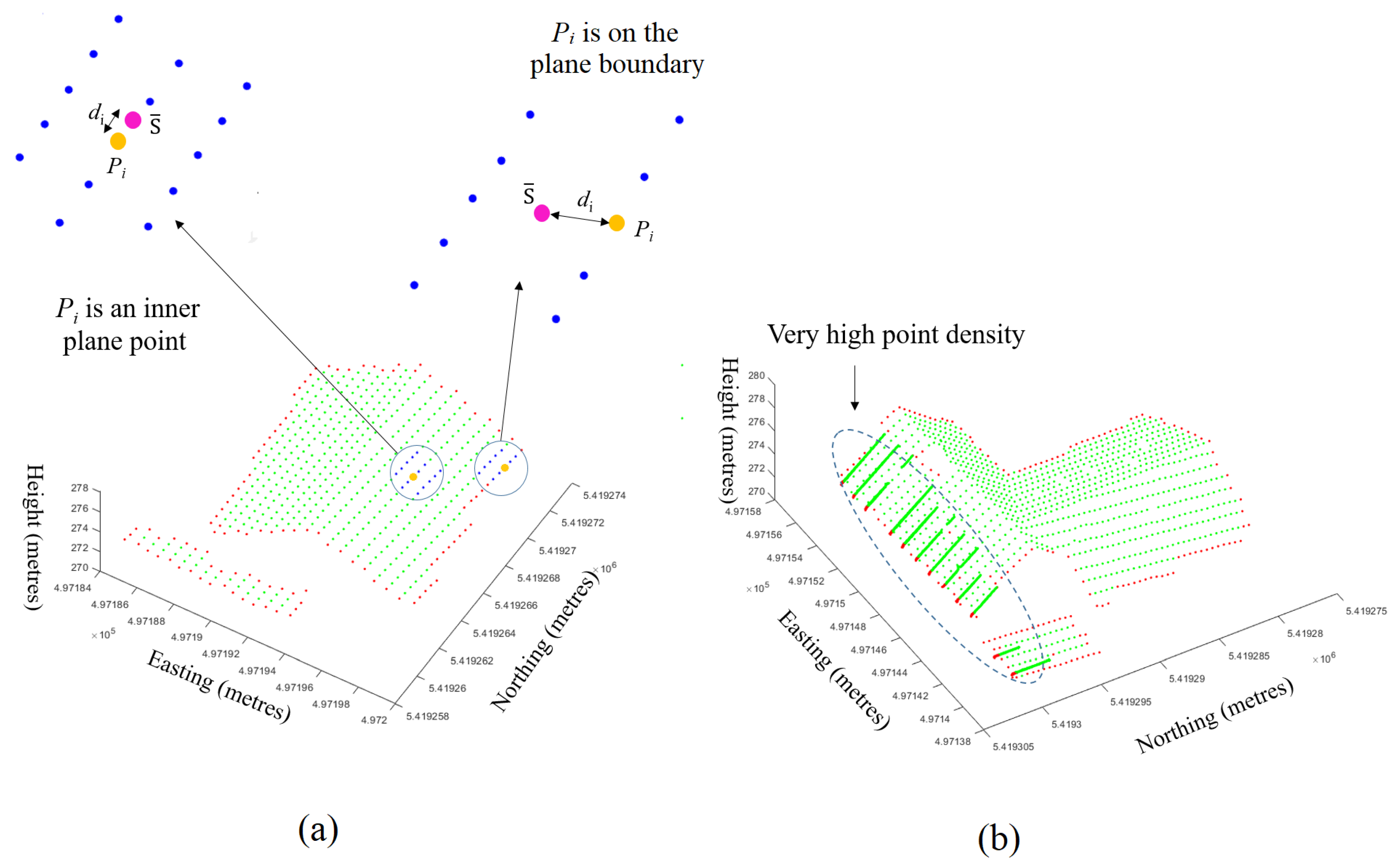
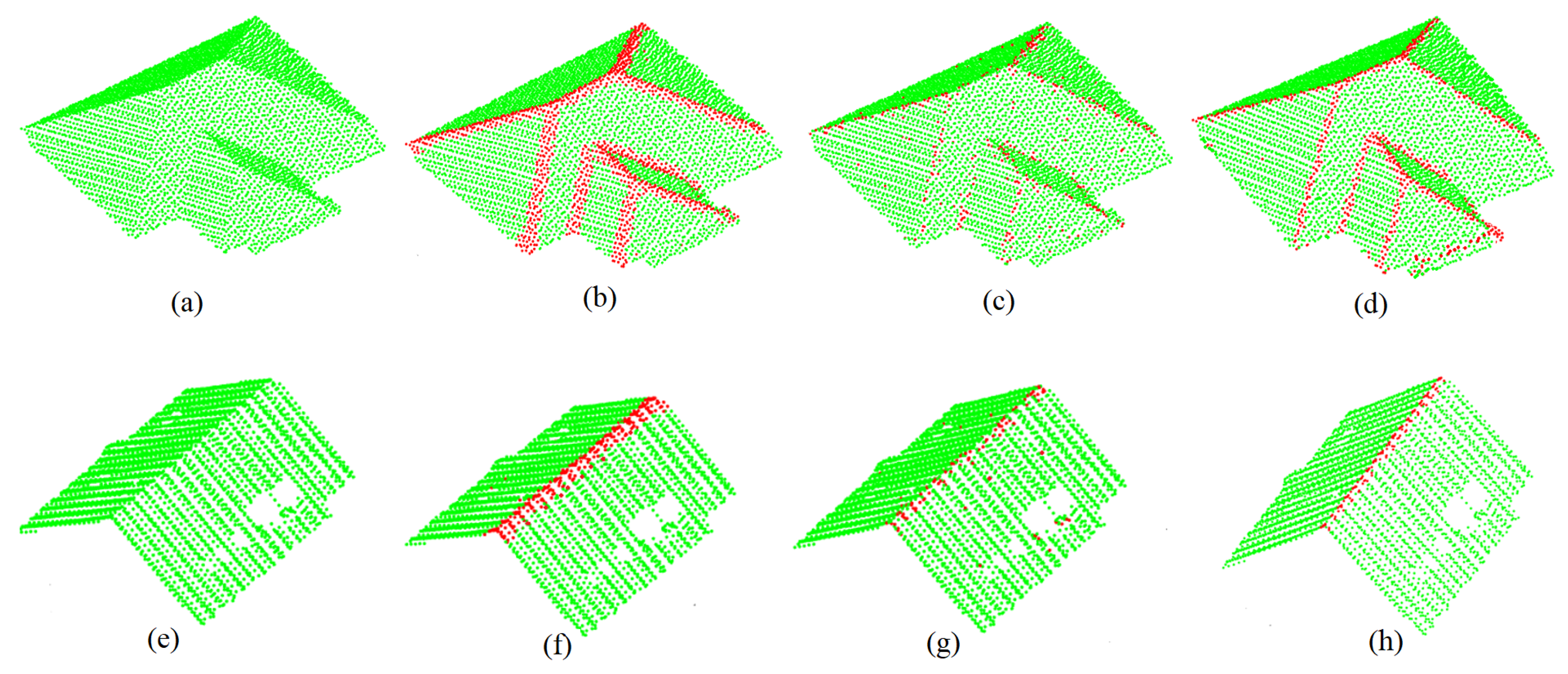
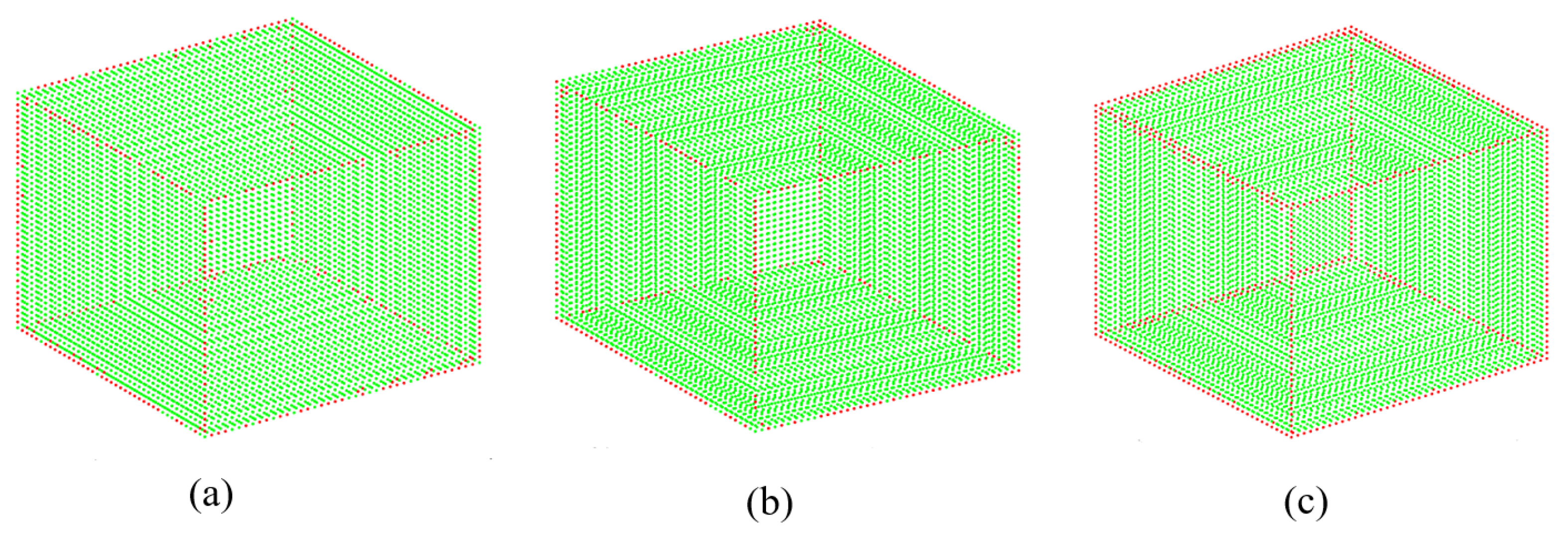
    T d = 1 ϑ
  • If σ i T d , S p is the estimated minimal neighbourhood for P i . The green points in Figure 3a show that the above steps successfully define the minimal neighbourhood for all points on a building roof. However, when there are unexpectedly a large number of points residing along a portion of a scanline, then these steps fail to define the neighbourhood, as in this case, all or most of the points in S p are obtained from the same scanline using the k-NN algorithm (see Figure 3b). Since points are not selected from two or more scanlines, the 3D line is repeatedly formed on the scanline that offers a low σ i value.
  • To avoid the above issue, this paper proposes a new neighbourhood search procedure for P i (see Figure 3c). First, depending on the input point density ϑ , when the number of points in S p is larger than A ϑ , where A is the area of the smallest detectable plane, points that are very close (e.g., ε = 0.01 m) to L 3 are removed from S p (blue points remain). Second, a line L passing through P i and perpendicular to L 3 (scanline) is generated. Third, a new rectangular neighbourhood C 1 C 2 C 3 C 4 (green shaded in Figure 3c) for P i is formed. C 1 C 2 C 3 C 4 is long along L but short along L 3 , and thus, the idea is to reduce the neighbouring points from the current scanline (blue points) and to include more points from outside the scanline (green points) and even from the next scanlines (yellow points). Finally, only six points closest to four corners and two midpoints ( C 1 , C 2 , C 3 , C 4 , M 1 , and M 2 ) from within C 1 C 2 C 3 C 4 and P i are assigned to an empty S p and σ i is again estimated to L 3 . If the condition ( σ i T d ) is still not satisfied, the rectangle is enlarged (orange shaded) along L to include more points from outside L 3 , i.e., four more points closest to corners C 5 , C 6 , C 7 , and C 8 are added to S p . It is experimentally observed that, when (mostly in the second iteration) points from the next scanlines are considered in S p , the condition is satisfied. Figure 3d shows that all points on the roof now have minimal neighbourhoods.
Airborne LiDAR data over a building roof follow the pattern of specific scanlines. The threshold T d for the standard deviation σ i provides the guarantee that points from at least two scanlines are selected for a minimal neighbourhood irrespective of the point density (e.g., abrupt high or diluted points). Thus, the calculated normal will be accurate as a true plane can be formed using the selected minimal neighbouring points. The variable nature of the proposed neighbourhood estimation solves existing issues with the normal calculation in the literature.

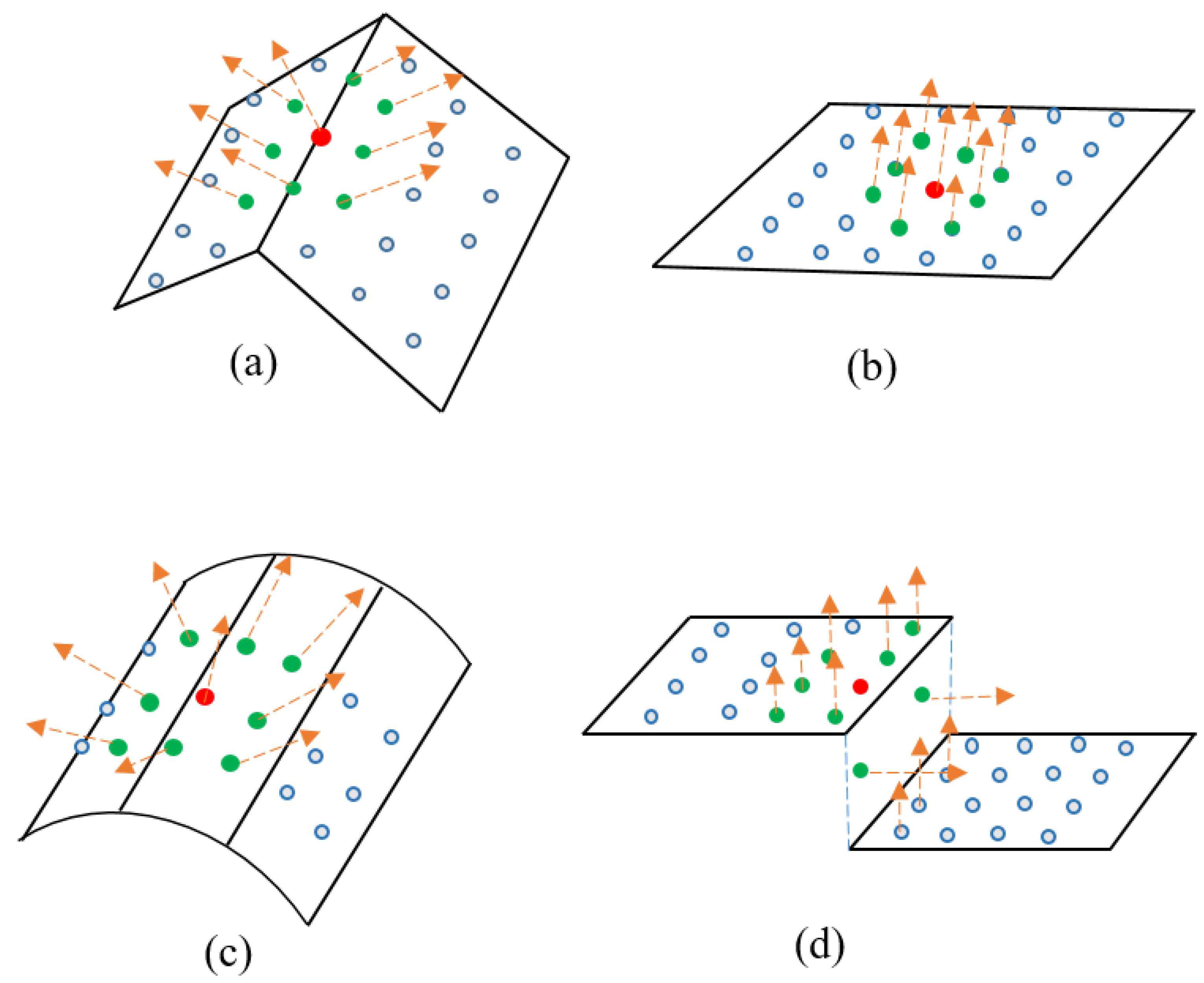
3.2. Finding Fold Points

The weighted PCA algorithm [60] is adopted to calculate the normal at each input point P i . The points within the minimal neighbourhood estimated above for P i are used to calculate its normal. This paper proposes the following method to determine the fold points.
To decide if P i is a fold point, the maximum angle difference θ max between its normal and the normals of its adjacent neighbours is found. Adjacent neighbours are simply obtained by using the k-NN algorithm from the selected neighbours S p for each point P i . An alternative to find the adjacent neighbours may be the Delaunay triangulation [61]. We consider at least 8 adjacent neighbours in this case. If the selected adjacent points from S p are less than 8, then we select the remaining adjacent points from the original point cloud. Figure 4 shows some cases to decide fold points with k = 8 . These cases are decided as follows by comparing θ max with an angle threshold T θ :
  • When two planes physically intersect, as shown in Figure 4a, and if θ max > T θ for P i (red dot) but θ max for its neighbours (green dots) can be clustered into two major groups, where the clusters are not close to each other, P i is a fold point.
  • When P i is a planar point, as shown in Figure 4b, θ max T θ for P i and all its neighbours.
  • When P i is on a curved surface, as shown in Figure 4c, θ max > T θ for P i and θ max for its neighbours are very close to T θ .
  • When P i is on a step edge, as shown in Figure 4d, there can be one of two situations. The adjacent vertical plane may have no or a small number of points. When there are no points on the vertical plane, then the fold points may be completely undetermined if the two planes (top and bottom) are parallel. If there is a large slope difference between these two planes, then the case in Figure 4a applies and fold points will be determined. When there are points reflected from the vertical plane, the fold points (between vertical and top planes and between vertical and bottom planes) can also be determined using the case in Figure 4a.

3.3. Determining the Threshold T θ

To determine the threshold T θ for θ max , we consider points on a simple building from the International Society for Photogrammetry and Remote Sensing (ISPRS) benchmark dataset presented in Figure 5. The ground truth for the fold and planar points are manually generated. A total of 138 points are identified as the fold points, and the rest (3421) of the points are considered planar points.
We consider different fixed neighbourhoods ( k = 9, 20, 30, 45, and 60) and the variable neighbourhood proposed in Section 3.1. For each neighbourhood considered, we estimate θ max for all the points. In Figure 5, these points are shown in different colours depending on their θ max values. As can be seen, while a small ( k = 9 ) or large ( k = 60 ) value of k misses many true fold points between the two building planes, a moderate value ( k = 45 ) of k determines most of the fold points but also wrongly identifies many planar points as fold points. In contrast, the proposed variable neighbourhood determines most of the fold and planar points truly. Table 1 shows that the proposed neighbourhood offers better F1-score [53] than the fixed neighbourhoods when we consider θ max 20 for the fold points.
We observe that θ max values of the ground truth fold points lie in the last two angle groups (20 to 30 and 30 to 90 ) of Table 1. The calculated F1-scores, considering only these two groups, as shown in the last row of the table, are highest among all possible combinations of groups of θ max for each neighbourhood. The planar points have θ max between 0 to 20 . Therefore, we decide T θ = 20 .
To prove this selection of T θ is insensitive to the input point density, we selected some representative buildings from different datasets with different point densities (i.e., five buildings from the ISPRS Vaihingen area, five from Hervey Bay, and five from Aitkenvale areas; see Section 4.1) and a synthetic cube shape point cloud (see Section 4.3). Besides this, we also generated different point densities by resampling the original point cloud [62]. Figure 6 shows the average values of θ max for the fold points under different point densities. It can be observed that T θ = 20 is a reasonable choice irrespective of different cases of point densities and datasets.

3.4. Detection of Boundary Points

We propose a simple but effective procedure for detection of the boundary points using the minimal neighbouring points S p for each P i . To make the decision about whether P i is on boundary, we first calculate the mean ( S ¯ ) of S p . Then, the Euclidean distance ( d i ) from S ¯ to P i is calculated. In practice, when P i is an inner point on the plane, S ¯ resides close to P i since the neighbouring points surround P i (see Figure 7a). However, when P i resides on the boundary, then S ¯ resides away from P i (i.e., the boundary) since there are no neighbouring points outside the boundary. Therefore, we use a threshold to distinguish the boundary and non-boundary points. P i is considered a boundary point when d i T d 2 , where T d is the threshold calculated based on the density of point cloud using Equation (3). Figure 7 shows the detected boundary points on two different roof point clouds. In Figure 7b, the proposed method can also extract the proper boundary points because S p rejects the much closed points and accepts only the suitable points for P i , as described in Section 3.1 using Figure 3c.

4. Experimental Results

Focusing on the extraction of feature points over the building roof, the proposed methods are applied on real point cloud datasets. We chose the extracted buildings from two different datasets. The first one is the Australian benchmark [7], and the second one is the International Society for Photogrammetry and Remote Sensing (ISPRS) benchmark dataset [62,63]. Buildings from two different sites of Australian datasets and three sites of the ISPRS datasets were selected for the evaluation. To extract and justify the point clouds over the building roof, we employed the results of the extracted building roofs from Dey et al. [7,53]. Moreover, to demonstrate and compare the quantitative evaluation of our methods with the existing state-of-the-arts techniques, we manually generated the ground truth for two areas from the two different datasets. A short description of the datasets and the ground truth is given below followed by the results of the comparative analysis and outline generation. Finally, the applicability of the proposed methods are also demonstrated on the point cloud generated or captured by different media, such as, artificially generated or terrestrially scanned data.

4.1. Datasets

The Australian datasets contain three sites from two different areas: Aitkenvale and Hervey Bay. Two sites from Aikenvale area (AV) have high point densities 12 to 40 points/m 2 . The first one (AV1) covers a 66 m × 52 m area and contains 5 different buildings. The second site (AV2) contains 63 different buildings covering an area of 214 m × 149 m. Hervey Bay (HB) has 28 different buildings covering 108 m × 104 m area by a medium point density (12 points/m 2 ). The ISPRS benchmark datasets have three different sites from the Vaihingen area (VH), containing a total of 107 buildings with different complexities and shapes. Point density of the datasets is low, 2.5 to 3.9 points/m 2 . The first site (VH1) of this area is mainly the inner city consisting of historic buildings. The second site (VH2) contains high-rising buildings, and the third site (VH3) is a residential area. Figure 8 shows the selected sites from two different datasets.
It is hard to collect the ground truth from the point cloud data. Hence, we selected AV1 and VH3 only because these two sites are purely residential with detached houses. The roof of the buildings of these two sites contain multiple planes; thus, sufficient fold points exist for the ground-truth generation and evaluation. We manually categorised the roof points of each building into three different categories: fold edge points, boundary points, and inner planar points. For a fold edge point, we kept the point within a maximum distance from the intersection line: 0.15 m for AV1 and 0.3 m for VH3. These two distances are estimated based on the point density according to the Equation (3).

4.2. Comparison

To calculate and compare the processing time of the proposed neighbourhood selection method, we chose all buildings from both AV1 and VH3 sites. Table 2 compares and summarises the average processing time per building of the proposed method for each datasets with different fixed-size neighbourhood. For AV1, the proposed method takes an average of 0.232 s to find the minimal neighbourhood for all points in a building, whereas the k-NN algorithm takes 0.058 s considering k = 45. For VH3 sites, the average processing time for the proposed method is 3.120 s. The influence of the variation of k on the processing time is negligible, as shown in Table 2. Due to the existence of an abrupt point density in several buildings, the average processing time increases for VH3 datasets. For example, the building we considered from VH3 in Figure 7b takes 42.94 s to find its minimal neighbourhood for all points using our proposed method. Finally, despite the considerable difference between the processing time values between the fixed-size and proposed variable-size neighbourhood selection methods, the processing time for the proposed minimal variable-size neighbourhood selection approach is still in the acceptable range. All experiments were performed in MATLAB 2020 platform using an Intel(R) core(TM) i5-7500 CPU at 3.40 GHz with 16 GB RAM.
To demonstrate the comparison, the performance of the proposed fold point extraction and the proposed boundary point extraction using the proposed neighbourhood selection method is compared with the existing state-of-the-art methods. Both qualitative and quantitative results are presented and compared.

4.2.1. Fold Points

To compare the performance of the proposed fold point extraction method, we chose the AGPN method proposed by Ni et al. [16] and the fold point extraction method proposed by Chen et al. [17]. Because they are not publicly available, we implemented these methods using MATLAB to evaluate and compare their performance on our datasets. To ensure reproduction of the implementation, we carefully followed the original articles and checked the results using similar data. We obtained almost the same results. Moreover, we were provided with partial codes and some sample data from the authors of the original articles (e.g., Figures 16 and 17). The general comparison between these two and the proposed methods is summarised in Table 3. Figure 9 shows the extracted fold edge points using these two methods along with our proposed method for two sample buildings from AV1 and VH3 sites for a qualitative comparison. It is clearly visible that the proposed method identifies the points belonging to the fold edge better than the AGPN and Chen methods. The AGPN method slightly outperforms the Chen method. This is because the AGPN extracts the fold points based on a model fitting and region growing approach and, thus, is more suitable for the objects containing planar parts. However, both of the existing methods extract a lot of false-positive (FP) fold points. In this case, our proposed method extracts more precise and accurate fold points, which are clearly visible in Figure 9d,h.
Using the generated ground truth of the AV1 and VH3 area, we evaluated and compared the quantitative performance of these three methods. We considered the precision, recall rates, and F1-score [53] as quantitative measures. Lower precision rates of the existing methods in Table 4 indicate that their FP rates are higher than that of the proposed method. The AGPN has a higher true positive rate, but as it considers the intersection area of two different planes, a wider fold edge is selected; thus, a lot of FP points are selected. The Chen method can select a narrow edge, but at the same time, it misclassifies many true planar points as the fold edge, which leads to a lower precision rate. A lower recall rate of the Chen method for both datasets indicates a higher false negative rate, which is also visible in Figure 9c,g. The F1-scores show that the proposed method performs better than both of the existing methods.

4.2.2. Boundary Points

The performance of the proposed boundary point extraction method is compared with the recently proposed approach by Chen et al. [17] and the improved RANSAC method proposed by Ni et al. [16].
Table 5 summarises the comparison among the methods, and Figure 10 shows the visual comparison using two sample buildings selected from the VH3 and AV2 sites. The building in the first row in Figure 10 is selected from the ISPRS benchmark site (VH3) and has a low point density, while the building of the second row is selected from a high-density Australian site (AV2). Figure 10a,d represent the results of the Chen method, where we can see that some boundary points are missed on the bottom roof plane. One possible reason for misclassifying the boundary points is that the Chen method projects the neighbouring points into a 2D plane; thus, it cannot differentiate the boundary between two separate planes in the same building. Again, from Figure 10b,e, we can see that the improved RANSAC method can extract the boundary points well, but a lot of non-boundary points are also classified as boundary points and some true boundary points are missed. The probable reason behind the misclassification is that the angle between the two projected vectors has two different values, and sometimes, the method cannot choose the correct one [17]. Our proposed method is able to correctly extract the boundary points for these two buildings, as shown in Figure 10c,f. Though some false-positive points are noticeable, these are much lower than the improved RANSAC method, and there are very few missing true boundary points.
To demonstrate the quantitative comparison, the extracted boundary points of the buildings from the AV1 and VH3 areas are evaluated using the generated ground truth. Table 6 compares the results of the extracted boundary points by three different methods. The Chen method has a higher precision rate because the FP rate is lower, which means fewer inner points are identified as boundaries. Again, as the projection of 3D neighbourhood into 2D limits the detection of some true boundary points, lower recall rate is noticeable for both datasets by the Chen method. However, it performs better than AGPN and F1-score for both datasets. The proposed method has a higher recall rate and F1-scores. Thus, the overall performance of the proposed boundary extraction is much better than the state-of-the-arts.

4.2.3. Eigenvalue-Based Features

Although there are several eigenvalue-based features in the literature to classify the LiDAR points into the fold edge and non-edge points, for simplicity and to demonstrate the applicability of the proposed neighbourhood selection method, we have chosen the frequently used parameters linearity ( L ) and planarity ( P ). Equations (1) and (2) are used to calculate these two features. To find the eigenvalues ( λ 1 , λ 2 , λ 3 ), the covariance matrix was constructed based on the information of the local neighbourhood. We demonstrate the qualitative performance of different fixed neighbourhoods against our proposed variable neighbourhood on a sample building from the ISPRS benchmark datasets.
In Figure 11, we calculated the linearity and planarity for each point. For a fair comparison, we considered a binary decision where green points indicate L ≥ 0.5 and red points indicate P ≥ 0.5. Blue points are considered as the original undecided points. It is clearly visible that, for low k values, both L and P found unexpected results (Figure 11a,b). A high k value considers the fold edge points as planar too (Figure 11e). It seems that, among all five k values, k = 45 (Figure 11c) shows an acceptable performance, where the proposed method allows almost similar performance for linear and planar points. Moreover, the proposed approach shows a clear distinction of the fold edge points (blue points in Figure 11f). To show the quantitative performance, F1 scores for the extracted linear and planar points are demonstrated in Table 7 for a different number of neighbouring points using the manually generated ground truth for the same building. Both fold and boundary points are considered as linear for simplicity.

4.2.4. Combined Results

Figure 12 shows the combined results of fold (blue), boundary (red), and planar (yellow) points for a sample complex building roof from the HB datasets. It is clearly visible that the combination of the proposed boundary, fold, and planar point extraction describes the building roof structure very well as it is almost similar to the reference 3D roof. Figure 13 shows the same for the AV1 dataset. Figure 14 also shows the same for some selected buildings from the AV2, HB, and VH areas. In all examples, a very small number of points, which are negligible as the total number of input points is a large number, are misclassified.

4.3. Applicability in Different Types of Point Clouds

In addition to the performance study using the real aerial point cloud data presented above, we also chose two other types of point cloud data. Firstly, a cubic object was selected as an example for artificially generated synthetic point cloud data [64] (Figure 15).
Secondly, a commercial building (Figure 16) and a structure of “3S” (Figure 17) used by Chen et al. [17] were selected as representatives of terrestrial laser scanning (TLS) data [17], with an average density of 4000 points/m 2 . The name of the commercial building is “Computer World” situated next to Wuhan University, and the “3S” structure is about 7 m tall with several flat and curved components situated within the university area.
In both of the cases, all thresholds of the proposed methods are selected in the same way described in Section 3. For the cube shape, Figure 15 compares the results by the three methods. To evaluate the quantitative performance, we calculate the number of actual fold edge points and then evaluate the different methods, which is demonstrated in Table 8. The total number of points and the true fold edge points in this shape are 9602 and 484, respectively. We chose a neighbourhood size of 20 for both the AGPN and Chen methods.
Figure 16 and Figure 17 show the results on the building TLS data by the three methods. We can see that the existing methods extract a lot of false fold and boundary points. However, the proposed method contains less false fold and boundary points. Table 9 and Table 10 demonstrate the quantitative comparison between three methods in terms of total extracted feature (boundary and fold) points for “Computer World” building and the “3S” structure, respectively. As ground truths are not available for these two structure, we follow the comparison technique used by Chen et al. [17] in this situation. The extraction rate for each structure depicts the performance. For both of the TLS datasets, we chose a neighbourhood size of 30 for the AGPN and Chen methods.

5. Conclusions

This paper proposes an approach for selecting the minimal variable neighbourhood for airborne LiDAR point cloud data over the building roof. The proposed approach solves the problem of accurate normal estimation for finding the fold edge points. To extract the boundary, an effective boundary point selection method is also proposed using the suggested neighbourhood selection method. The proposed neighbourhood selection method is independent of various point densities and the calculation of normal vectors are not influenced by the heterogenic distribution of the point cloud. Using the generated ground truth for the two selected areas from the ISPRS and Australian benchmark datasets, we show the applicability and performance of the proposed method. Two different types of point cloud data, such as, artificially generated and terrestrially scanned, are also tested using the proposed methods.
In this research, we focused mainly on feature point extraction from point cloud data, which follow a specific scanline pattern. Thus, the methods are mainly demonstrated and most of the experiments are performed on the standard benchmark data of the building roof point cloud. We considered the building roof point cloud extracted from the original point cloud datasets in this research. Vegetation, outliers, and other objects were removed using our previously developed methods of building extraction. However, integrating some machine learning techniques may improve these proposed methods in terms of selecting manual thresholds. Tracing feature lines from the extracted feature points is the next step of 3D reconstruction. In the future, we will investigate the incorporation of machine learning techniques to extract the feature points and an effective feature line tracing algorithm to regularise the extracted feature points. Moreover, the applicability of the proposed methods will also be investigated in different application areas such as 3D modelling of indoor objects.

Author Contributions

Conceptualization, E.K.D.; methodology, E.K.D.; software, E.K.D., F.T.K.; validation, E.K.D.; formal analysis, E.K.D.; investigation, E.K.D., F.T.K.; resources, F.T.K., M.A.; data curation, E.K.D., F.T.K., M.A.; writing—original draft preparation, E.K.D.; writing—review and editing, E.K.D., F.T.K., M.A., B.S.; visualization, E.K.D., M.A.; supervision, M.A., B.S., F.T.K. All authors have read and agreed to the published version of the manuscript.

Funding

This research received no external funding.

Acknowledgments

The authors wish to acknowledge support from the School of Information and Communication Technology, Griffith University, Australia, also like to thank Xijiang Chen for providing the point cloud data of the “3S” structure and “Computer World” building. The ISPRS datasets was provided by the German Society for Photogrammetry, Remote Sensing and Geoinformation (DGPF).

Conflicts of Interest

The authors declare no conflict of interest.

References

  1. Koch, T.; Korner, M.; Fraundorfer, F. Automatic alignment of indoor and outdoor building models using 3D line segments. In Proceedings of the IEEE Conference on Computer Vision and Pattern Recognition Workshops, Las Vegas, NV, USA, 27–30 June 2016; pp. 10–18. [Google Scholar]
  2. Kang, Z.; Zhong, R.; Wu, A.; Shi, Z.; Luo, Z. An efficient planar feature fitting method using point cloud simplification and threshold-independent BaySAC. IEEE Geosci. Remote Sens. Lett. 2016, 13, 1842–1846. [Google Scholar] [CrossRef]
  3. Yang, B.; Fang, L.; Li, J. Semi-automated extraction and delineation of 3D roads of street scene from mobile laser scanning point clouds. ISPRS J. Photogramm. Remote Sens. 2013, 79, 80–93. [Google Scholar] [CrossRef]
  4. Poullis, C. A framework for automatic modeling from point cloud data. IEEE Trans. Pattern Anal. Mach. Intell. 2013, 35, 2563–2575. [Google Scholar] [CrossRef] [PubMed]
  5. Albano, R. Investigation on Roof Segmentation for 3D Building Reconstruction from Aerial LIDAR Point Clouds. Appl. Sci. 2019, 9, 4674. [Google Scholar] [CrossRef] [Green Version]
  6. Tarsha Kurdi, F.; Awrangjeb, M. Automatic evaluation and improvement of roof segments for modelling missing details using Lidar data. Int. J. Remote Sens. 2020, 41, 4702–4725. [Google Scholar] [CrossRef]
  7. Dey, E.K.; Awrangjeb, M.; Stantic, B. Outlier detection and robust plane fitting for building roof extraction from LiDAR data. Int. J. Remote. Sens. 2020, 41, 6325–6354. [Google Scholar] [CrossRef]
  8. Sanchez, J.; Denis, F.; Dupont, F.; Trassoudaine, L.; Checchin, P. Data-driven modeling of building interiors from lidar point clouds. ISPRS Ann. Photogramm. Remote Sens. Spat. Inf. Sci. 2020, 2, 395–402. [Google Scholar] [CrossRef]
  9. Lafarge, F.; Mallet, C. Creating large-scale city models from 3D-point clouds: a robust approach with hybrid representation. Int. J. Comput. Vis. 2012, 99, 69–85. [Google Scholar] [CrossRef]
  10. Sampath, A.; Shan, J. Segmentation and reconstruction of polyhedral building roofs from aerial lidar point clouds. IEEE Trans. Geosci. Remote Sens. 2009, 48, 1554–1567. [Google Scholar] [CrossRef]
  11. Ni, H.; Lin, X.; Zhang, J. Applications of 3d-edge detection for ALS point cloud. Int. Arch. Photogramm. Remote Sens. Spat. Inf. Sci. 2017, 42. [Google Scholar] [CrossRef] [Green Version]
  12. Awrangjeb, M.; Gilani, S.A.N.; Siddiqui, F.U. An effective data-driven method for 3-d building roof reconstruction and robust change detection. Remote Sens. 2018, 10, 1512. [Google Scholar] [CrossRef] [Green Version]
  13. Balado, J.; Arias, P.; Díaz-Vilariño, L.; González-deSantos, L.M. Automatic CORINE land cover classification from airborne LIDAR data. Procedia Comput. Sci. 2018, 126, 186–194. [Google Scholar] [CrossRef]
  14. Tarsha-Kurdi, F.; Landes, T.; Grussenmeyer, P. Extended RANSAC algorithm for automatic detection of building roof planes from LiDAR data. Photogramm. J. Finl. 2008, 21, 97–109. [Google Scholar]
  15. Awrangjeb, M.; Zhang, C.; Fraser, C.S. Automatic extraction of building roofs using LIDAR data and multispectral imagery. ISPRS J. Photogramm. Remote Sens. 2013, 83, 1–18. [Google Scholar] [CrossRef] [Green Version]
  16. Ni, H.; Lin, X.; Ning, X.; Zhang, J. Edge detection and feature line tracing in 3d-point clouds by analyzing geometric properties of neighborhoods. Remote Sens. 2016, 8, 710. [Google Scholar] [CrossRef] [Green Version]
  17. Chen, X.; Yu, K. Feature line generation and regularization from point clouds. IEEE Trans. Geosci. Remote Sens. 2019, 57, 9779–9790. [Google Scholar] [CrossRef]
  18. Zhang, Y.; Geng, G.; Wei, X.; Zhang, S.; Li, S. A statistical approach for extraction of feature lines from point clouds. Comput. Graph. 2016, 56, 31–45. [Google Scholar] [CrossRef]
  19. Vosselman, G.; Dijkman, S. 3D building model reconstruction from point clouds and ground plans. Int. Arch. Photogramm. Remote Sens. Spat. Inf. Sci. 2001, 34, 37–44. [Google Scholar]
  20. Demarsin, K.; Vanderstraeten, D.; Volodine, T.; Roose, D. Detection of closed sharp edges in point clouds using normal estimation and graph theory. Comput. Aided Des. 2007, 39, 276–283. [Google Scholar] [CrossRef]
  21. Bazazian, D.; Casas, J.R.; Ruiz-Hidalgo, J. Fast and robust edge extraction in unorganized point clouds. In Proceedings of the 2015 International Conference on Digital Image Computing: Techniques and Applications (DICTA), Adelaide, Australia, 23–25 November 2015; pp. 1–8. [Google Scholar]
  22. Yang, L.; Sheng, Y.; Wang, B. 3D reconstruction of building facade with fused data of terrestrial LiDAR data and optical image. Optik 2016, 127, 2165–2168. [Google Scholar] [CrossRef]
  23. Wang, Z.; Prisacariu, V.A. Neighbourhood-Insensitive Point Cloud Normal Estimation Network. arXiv 2020, arXiv:2008.09965. [Google Scholar]
  24. Sanchez, J.; Denis, F.; Coeurjolly, D.; Dupont, F.; Trassoudaine, L.; Checchin, P. Robust normal vector estimation in 3D point clouds through iterative principal component analysis. ISPRS J. Photogramm. Remote Sens. 2020, 163, 18–35. [Google Scholar] [CrossRef] [Green Version]
  25. Zhu, Q.; Wang, F.; Hu, H.; Ding, Y.; Xie, J.; Wang, W.; Zhong, R. Intact planar abstraction of buildings via global normal refinement from noisy oblique photogrammetric point clouds. ISPRS Int. J. Geo-Inf. 2018, 7, 431. [Google Scholar] [CrossRef] [Green Version]
  26. Zhao, R.; Pang, M.; Liu, C.; Zhang, Y. Robust normal estimation for 3D LiDAR point clouds in urban environments. Sensors 2019, 19, 1248. [Google Scholar] [CrossRef] [PubMed] [Green Version]
  27. Leichter, A.; Werner, M.; Sester, M. Feature-extraction from all-scale neighborhoods with applications to semantic segmentation of point clouds. Int. Arch. Photogramm. Remote Sens. Spat. Inf. Sci. 2020, 43, 263–270. [Google Scholar] [CrossRef]
  28. Ben-Shabat, Y.; Lindenbaum, M.; Fischer, A. Nesti-net: Normal estimation for unstructured 3d point clouds using convolutional neural networks. In Proceedings of the IEEE Conference on Computer Vision and Pattern Recognition, Long Beach, CA, USA, 16–20 June 2019; pp. 10112–10120. [Google Scholar]
  29. He, E.; Chen, Q.; Wang, H.; Liu, X. A curvature based adaptive neighborhood for individual point cloud classification. Int. Arch. Photogramm. Remote Sens. Spat. Inf. Sci. 2017, 42. [Google Scholar] [CrossRef] [Green Version]
  30. Weinmann, M.; Jutzi, B.; Hinz, S.; Mallet, C. Semantic point cloud interpretation based on optimal neighborhoods, relevant features and efficient classifiers. ISPRS J. Photogramm. Remote Sens. 2015, 105, 286–304. [Google Scholar] [CrossRef]
  31. Weinmann, M.; Jutzi, B.; Mallet, C. Semantic 3D scene interpretation: A framework combining optimal neighborhood size selection with relevant features. ISPRS Ann. Photogramm. Remote Sens. Spat. Inf. Sci. 2014, 2, 181. [Google Scholar] [CrossRef] [Green Version]
  32. Shannon, C.E. A mathematical theory of communication. Bell Syst. Tech. J. 1948, 27, 379–423. [Google Scholar] [CrossRef] [Green Version]
  33. Ben-Shabat, Y.; Lindenbaum, M.; Fischer, A. 3dmfv: Three-dimensional point cloud classification in real-time using convolutional neural networks. IEEE Robot. Autom. Lett. 2018, 3, 3145–3152. [Google Scholar] [CrossRef]
  34. Weinmann, M.; Jutzi, B.; Mallet, C. Feature relevance assessment for the semantic interpretation of 3D point cloud data. ISPRS Ann. Photogramm. Remote Sens. Spat. Inf. Sci. 2013, 5, 1. [Google Scholar] [CrossRef] [Green Version]
  35. Hughes, G. On the mean accuracy of statistical pattern recognizers. IEEE Trans. Inf. Theory 1968, 14, 55–63. [Google Scholar] [CrossRef] [Green Version]
  36. Weber, C.; Hahmann, S.; Hagen, H.; Bonneau, G.P. Sharp feature preserving MLS surface reconstruction based on local feature line approximations. Graph. Model. 2012, 74, 335–345. [Google Scholar] [CrossRef] [Green Version]
  37. Nurunnabi, A.; West, G.; Belton, D. Outlier detection and robust normal-curvature estimation in mobile laser scanning 3D point cloud data. Pattern Recognit. 2015, 48, 1404–1419. [Google Scholar] [CrossRef] [Green Version]
  38. Dey, T.K.; Li, G.; Sun, J. Normal estimation for point clouds: A comparison study for a Voronoi based method. In Proceedings of the Eurographics/IEEE VGTC Symposium Point-Based Graphics, Brook, NY, USA, 21–22 June 2005; pp. 39–46. [Google Scholar]
  39. Pauly, M.; Gross, M.; Kobbelt, L.P. Efficient simplification of point-sampled surfaces. In Proceedings of the IEEE Visualization, Boston, MA, USA, 27 October–1 November 2002; pp. 163–170. [Google Scholar]
  40. Alexa, M.; Behr, J.; Cohen-Or, D.; Fleishman, S.; Levin, D.; Silva, C.T. Computing and rendering point set surfaces. IEEE Trans. Vis. Comput. Graph. 2003, 9, 3–15. [Google Scholar] [CrossRef] [Green Version]
  41. Hubert, M.; Rousseeuw, P.J.; Vanden Branden, K. ROBPCA: A new approach to robust principal component analysis. Technometrics 2005, 47, 64–79. [Google Scholar] [CrossRef]
  42. Nurunnabi, A.; Belton, D.; West, G. Diagnostic-robust statistical analysis for local surface fitting in 3D point cloud data. ISPRS Ann. Photogramm. Remote Sens. Spat. Inf. Sci. 2012, 269–274. [Google Scholar] [CrossRef] [Green Version]
  43. Dey, E.K.; Awrangjeb, M.; Stantic, B. An Unsupervised Outlier Detection Method For 3D Point Cloud Data. In Proceedings of the 2019 IEEE International Geoscience and Remote Sensing Symposium, Yokohama, Japan, 28 July–2 August 2019; pp. 2495–2498. [Google Scholar]
  44. Huber, P.J. Robust Statistics. In International Encyclopedia of Statistical Science; Lovric, M., Ed.; Springer: Berlin/Heidelberg, Germany, 2011; pp. 1248–1251. [Google Scholar]
  45. Kanungo, T.; Mount, D.M.; Netanyahu, N.S.; Piatko, C.D.; Silverman, R.; Wu, A.Y. An efficient k-means clustering algorithm: Analysis and implementation. IEEE Trans. Pattern Anal. Mach. Intell. 2002, 24, 881–892. [Google Scholar] [CrossRef]
  46. Guennebaud, G.; Gross, M. Algebraic point set surfaces. In ACM Siggraph 2007 Papers; ACM: New York, NY, USA, 2007. [Google Scholar]
  47. Lu, X.; Liu, Y.; Li, K. Fast 3D line segment detection from unorganized point cloud. arXiv 2019, arXiv:1901.02532. [Google Scholar]
  48. Xu, S.; Wang, R.; Zheng, H. Road curb extraction from mobile LiDAR point clouds. IEEE Trans. Geosci. Remote Sens. 2016, 55, 996–1009. [Google Scholar] [CrossRef] [Green Version]
  49. Lin, Y.; Wang, C.; Cheng, J.; Chen, B.; Jia, F.; Chen, Z.; Li, J. Line segment extraction for large scale unorganized point clouds. ISPRS J. Photogramm. Remote Sens. 2015, 102, 172–183. [Google Scholar] [CrossRef]
  50. Ge, X. Automatic markerless registration of point clouds with semantic-keypoint-based 4-points congruent sets. ISPRS J. Photogramm. Remote Sens. 2017, 130, 344–357. [Google Scholar] [CrossRef] [Green Version]
  51. Moghadam, P.; Bosse, M.; Zlot, R. Line-based extrinsic calibration of range and image sensors. In Proceedings of the 2013 IEEE International Conference on Robotics and Automation, Karlsruhe, Germany, 6–10 May 2013; pp. 3685–3691. [Google Scholar]
  52. Xia, S.; Wang, R. A fast edge extraction method for mobile LiDAR point clouds. IEEE Geosci. Remote Sens. Lett. 2017, 14, 1288–1292. [Google Scholar] [CrossRef]
  53. Dey, E.K.; Awrangjeb, M. A Robust Performance Evaluation Metric for Extracted Building Boundaries From Remote Sensing Data. IEEE J. Sel. Top. Appl. Earth Obs. Remote Sens. 2020, 13, 4030–4043. [Google Scholar] [CrossRef]
  54. Lu, Z.; Baek, S.; Lee, S. Robust 3d line extraction from stereo point clouds. In Proceedings of the 2008 IEEE Conference on Robotics, Automation and Mechatronics, Chengdu, China, 21–24 September 2008; pp. 1–5. [Google Scholar]
  55. Gumhold, S.; Wang, X.; MacLeod, R.S. Feature Extraction from Point Clouds; Citeseer: State College, PA, USA, 2001; pp. 293–305. [Google Scholar]
  56. Ioannou, Y.; Taati, B.; Harrap, R.; Greenspan, M. Difference of normals as a multi-scale operator in unorganized point clouds. In Proceedings of the 2012 Second International Conference on 3D Imaging, Modeling, Processing, Visualization & Transmission, Zurich, Switzerland, 13–15 October 2012; pp. 501–508. [Google Scholar]
  57. Belton, D.; Lichti, D.D. Classification and segmentation of terrestrial laser scanner point clouds using local variance information. Int. Arch. Photogramm. Remote Sens. Spat. Inf. Sci 2006, 36, 44–49. [Google Scholar]
  58. Santos, R.C.d.; Galo, M.; Tachibana, V.M. Classification of LiDAR data over building roofs using k-means and principal component analysis. Boletim de Ciências Geodésicas 2018, 24, 69–84. [Google Scholar] [CrossRef] [Green Version]
  59. Tarsha-Kurdi, F.; Landes, T.; Grussenmeyer, P.; Smigiel, E. New approach for automatic detection of buildings in airborne laser scanner data using first echo only. In Proceedings of the ISPRS Commission III Symposium, Photogrammetric Computer Vision, Bonn, Germany, 13 September 2006; pp. 25–30. [Google Scholar]
  60. Cochran, R.N.; Horne, F.H. Statistically weighted principal component analysis of rapid scanning wavelength kinetics experiments. Anal. Chem. 1977, 49, 846–853. [Google Scholar] [CrossRef]
  61. Awrangjeb, M. Using point cloud data to identify, trace, and regularize the outlines of buildings. Int. J. Remote Sens. 2016, 37, 551–579. [Google Scholar] [CrossRef]
  62. Awrangjeb, M.; Fraser, C.S. Automatic segmentation of raw LiDAR data for extraction of building roofs. Remote Sens. 2014, 6, 3716–3751. [Google Scholar] [CrossRef] [Green Version]
  63. Cramer, M. The DGPF test on digital aerial camera evaluation–overview and test design. Photogrammetrie–Fernerkundung–Geoinformation 2, 73–82 (2010). In Proceedings of the IEEE International Conference on Computer Vision, Santiago, Chile, 7–13 December 2015; pp. 1026–1034. [Google Scholar]
  64. Alexiou, E.; Ebrahimi, T. Benchmarking of objective quality metrics for colorless point clouds. In Proceedings of the 2018 Picture Coding Symposium (PCS), San Francisco, CA, USA, 24–27 June 2018; pp. 51–55. [Google Scholar]
Figure 1. Light Detection and Ranging (LiDAR) points over a building roof with scanning direction (red arrows).
Remotesensing 13 01520 g001
Figure 2. The workflow of the proposed variable neighbourhood selection method: T d is the threshold, σ i is the standard deviation, ε is the distance error, and δ is the neighbourhood increment.
Remotesensing 13 01520 g002
Figure 3. New neighbourhood search across the scanline: (a) a successfully defined minimal neighbourhood in a building where points are regularly distributed, (b) the red points indicate that minimal neighbourhoods could not be defined, (c) a rectangular neighbourhood is iteratively formed, and (d) a successfully defined neighbourhood after applying the technique described using (c).
Remotesensing 13 01520 g003
Figure 4. Cases to decide fold points P i (red dots). Their adjacent points are shown by green dots. Arrows indicate normal directions. (a) Gable roof, (b) planar surface, (c) curved surface, and (d) step edge between planes.
Remotesensing 13 01520 g004
Figure 5. Calculated θ max for different neighbourhoods: (a) k = 9 , (b) k = 20 , (c) k = 30 , (d) k = 45 , (e) k = 60 , and (f) the proposed neighbourhood.
Remotesensing 13 01520 g005
Figure 6. Average θ max values for the fold points under different point densities.
Remotesensing 13 01520 g006
Figure 7. Boundary point detection examples with (a) the usual point density on all planes and (b) the unexpectedly very high point density on some planes. In the magnified images of (a), d i indicates the distance between P i and the mean S ¯ of the neighbours S p .
Remotesensing 13 01520 g007
Figure 8. Used datasets for experiments. The first row shows the selected three sites from Australian datasets: (a) AV1, (b) HB, and (c) AV2. The second row indicates the three areas from the International Society for Photogrammetry and Remote Sensing (ISPRS) benchmark dataset: (d) VH1, (e) VH2 and (f) VH3. Buildings enclosed by the red line areas are taken into consideration for the ISPRS benchmark.
Remotesensing 13 01520 g008
Figure 9. Extracted fold edge points: (a,e) original building point cloud, (b,f) Analyzing Geometric Properties of Neighbourhood (AGPN) method [16], (c,g) Chen method [17], and (d,h) Proposed method.
Remotesensing 13 01520 g009
Figure 10. Extracted boundary points by (a,d) the Chen method [17], (b,e) the improved RANSAC method [16], and (c,f) the proposed method.
Remotesensing 13 01520 g010
Figure 11. Linear (red), planar (green), and fold edge (blue) points using the fixed k-NN and the proposed variable neighbourhood: (a) k = 9 , (b) k = 30 , (c) k = 45 , (d) k = 60 , (e) k = 90 , and (f) the proposed neighbourhood.
Remotesensing 13 01520 g011
Figure 12. Combined fold (blue), boundary (red,) and planar (yellow) points compared with the reference 3D building roof [7] for a complex building from the HB dataset: (a) reference 3D building roof and (b) combined result.
Remotesensing 13 01520 g012
Figure 13. Combined fold (blue), boundary (red), and planar (yellow) points compared with the reference 3D building roof [7] for all five buildings from the AV1 dataset: (a) reference 3D building roofs and (b) combined results.
Remotesensing 13 01520 g013
Figure 14. Combined fold (blue), boundary (red), and planar (yellow) points compared with the reference 3D building roof [7] for several buildings from the test datasets. While the first, third, and fifth rows show the reference information overlaid onto of the building roofs, the second, fourth, and sixth rows show the extracted results by the proposed method.
Remotesensing 13 01520 g014
Figure 15. Comparing results on a synthetic cube shape by the (a) AGPN [16], (b) Chen [17], and (c) proposed methods. Green represents planar points, and red represents fold points.
Remotesensing 13 01520 g015
Figure 16. Comparing results on building data by the (a) AGPN [16], (b) Chen [17], and (c) proposed methods. Green indicates the planar points, and red represents both the boundary and the fold edge points.
Remotesensing 13 01520 g016
Figure 17. Comparing the results on the “3S” structure of Wuhan University: (a) original point cloud, (b) extracted feature points using AGPN [16], (c) extracted feature points using Chen’s method [17] (d) extracted feature points using the proposed methods. the (e) extracted feature and planar points. Green indicates the planar points, and red represents both the boundary and the fold edge points.
Remotesensing 13 01520 g017
Table 1. Comparison of different fixed neighbourhoods with our proposed method.
θ max Number of Neighbouring PointsProposed Method
920304580
0–2 78326022793289528512465
2–10 2378620380285331765
10–20 178109224276371161
20–30 581671521036135
30–90 16261100023
F1-Score0.710.750.770.680.500.90
Table 2. Average processing time (in seconds) of neighbourhood selection techniques for each building.
Datasetsk-NN (k = 30)k-NN (k = 45)k-NN (k = 60)Proposed
VH30.0900.0910.0933.120
AV10.0580.0580.0600.232
Table 3. Comparison of different methods for fold edge point extraction.
AGPN [16]Chen [17]Proposed
NeighbourhoodFixed k-NNFixed k-NNVariable
Extraction approachPlane fitting and angular gapMinimal number of clusters of neighbouring normal vectorsMaximum angle difference of the calculated normal vectors
Normal estimationRANSACWeighted PCAWeighted PCA
Geometric propertyThe RANSAC and angular gap metricDirection of k-nearest normal vectorsMaximum angle differences among k-nearest normal
Plane fittingRequiredNot requiredNot required
Table 4. Quantitative comparison of the extracted fold edge points.
ISPRS Site (VH3)Australian Site (AV1)
PrecisionRecallF1PrecisionRecallF1
AGPN [16]0.670.840.750.780.760.77
Chen [17]0.740.790.770.750.730.74
Proposed0.790.870.830.840.850.84
Table 5. Comparison of different boundary point extraction methods.
Improved RANSAC [16]Chen [17]Proposed
Neighbourhood k d -treeFixed k-NNVariable
Decision of boundary pointSubstantial angular gap between vectors in a single planeDistribution of azimuth angleEuclidian distance from mean point to the point of interest
Plane fittingRequiredRequiredNot required
Effect of outliersHigh sensitiveLow sensitiveLow sensitive
Table 6. Quantitative comparison of the extracted boundary points.
ISPRS Site (VH3)Australian Site (AV1)
PrecisionRecallF1PrecisionRecallF1
Improved RANSAC [16]0.800.730.760.850.800.82
Chen [17]0.840.720.780.960.750.84
Proposed0.820.820.830.940.870.90
Table 7. Quantitative comparison of linearity and planarity for different neighbourhoods.
Values of
k
No. of Linear Points
L ≥ 0.5
No. of Planar Points
P ≥ 0.5
F1
(Linearity)
F1
(Planarity)
9243411150.190.15
30173918100.610.68
4557129780.840.88
6070528440.710.79
9084327060.750.84
Proposed40931400.910.94
Table 8. Comparing results on the cube shape.
Total Extracted PointsPrecisionRecallF1
AGPN [16]4040.920.800.85
Chen [17]3310.960.670.78
Proposed5970.821.000.90
Table 9. Comparison of the extracted feature (fold and boundary) points using the three methods for “Computer World” building.
Original Point CloudOutline PointsExtraction Rate
AGPN Method29,339598920.4%
Chen’s Method29,339509717.4%
Proposed29,339420314.3%
Table 10. Comparison of the extracted feature (fold and boundary) points using the three methods for the “3S” structure.
Original Point CloudOutline PointsExtraction Rate
AGPN Method53,96351469.50%
Chen’s Method53,963915016.95%
Proposed53,963606111.23%
Publisher’s Note: MDPI stays neutral with regard to jurisdictional claims in published maps and institutional affiliations.

