Article

Use of Sentinel-2 Satellite Data for Windthrows Monitoring and Delimiting: The Case of “Vaia” Storm in Friuli Venezia Giulia Region (North-Eastern Italy)

by
Valentina Olmo
1,2,
Enrico Tordoni
3,
Francesco Petruzzellis
1,2,
Giovanni Bacaro
2,* and
Alfredo Altobelli
2
1
Department of Agricultural, Food, Environmental and Animal Sciences, University of Udine, Via delle Scienze 206, 33100 Udine, Italy
2
Department of Life Science, University of Trieste, Via L. Giorgieri 10, 34127 Trieste, Italy
3
Department of Botany, Institute of Ecology and Earth Sciences, University of Tartu, Lai 40, 51005 Tartu, Estonia
*
Author to whom correspondence should be addressed.
Submission received: 21 March 2021 / Revised: 6 April 2021 / Accepted: 7 April 2021 / Published: 15 April 2021
(This article belongs to the Special Issue Feature Paper Special Issue on Ecological Remote Sensing)

Abstract

:
On the 29th of October 2018, a storm named “Vaia” hit North-Eastern Italy, causing the loss of 8 million m3 of standing trees and creating serious damage to the forested areas, with many economic and ecological implications. This event brought up the necessity of a standard procedure for windthrow detection and monitoring based on satellite data as an alternative to foresters’ fieldwork. The proposed methodology was applied in Carnic Alps (Friuli Venezia Giulia, NE Italy) in natural stands dominated by Picea abies and Abies alba. We used images from the Sentinel-2 mission: 1) to test vegetation indices performance in monitoring the vegetation dynamics in the short period after the storm, and 2) to create a windthrow map for the whole Friuli Venezia Giulia region. Results showed that windthrows in forests have a significant influence on visible and short-wave infrared (SWIR) spectral bands of Sentinel-2, both in the short and the long-term timeframes. NDWI8A and NDWI were the best indices for windthrow detection (R2 = 0.80 and 0.77, respectively) and NDVI, PSRI, SAVI and GNDVI had an overall good performance in spotting wind-damaged areas (R2 = 0.60–0.76). Moreover, these indices allowed to monitor post-Vaia forest die-off and showed a dynamic recovery process in cleaned sites. The NDWI8A index, employed in the vegetation index differencing (VID) change detection technique, delimited damaged areas comparable to the estimations provided by Regional Forest System (2545 ha and 3183 ha, respectively). Damaged forests detected by NDWI8A VID ranged from 500 m to 1500 m a.s.l., mainly covering steep slopes in the south and east aspects (42% and 25%, respectively). Our results suggested that the NDWI8A VID method may be a cost-effective and accurate way to produce windthrow maps, which could limit the risks associated with fieldwork and may provide a valuable tool to plan tree removal interventions in a more efficient way.

Graphical Abstract

1. Introduction

The recent growth of satellite technology in the field of Earth observation allows the measurement of electromagnetic radiation with a higher spatial, temporal and radiometric resolution, being potentially useful to detect environmental disturbances caused by natural hazards [1,2]. This feature is particularly relevant considering future scenarios where extreme natural events and their impacts are expected to become more frequent and intense [3]. As a term of reference, more than half of the total recorded damages to European forested areas has been caused by extraordinary events of extremely intense winds as a consequence of the ongoing climate change, whose associated damage levels are steeply increasing [4].
In the future, there are several factors that could increase forest vulnerability to storms: among these, increased intensity of heavy storms and winds, changes to storm tracks, higher air temperature and precipitations during winter and, finally, an increased pathogen activity triggered by higher temperatures [4]. During the last centuries, moderate biotic and abiotic disturbances played a key role in European forest ecosystem dynamics, stimulating regeneration and ecological succession processes and having positive effects on biological diversity [5]. However, high-intensity disturbances can be catastrophic and have complex repercussions on the biosphere, such as diminishing ecosystem functions, reducing biodiversity and altering land-atmosphere feedbacks through changes in forest structure and its physiologic processes [6]. The susceptibility of individual trees and tree stands to wind damage, and its mechanism, is determined by the properties of the wind climate (wind speed, gust speed, duration), forest structure (e.g., fragmentation and age), tree/stand characteristics (e.g., species, height, diameter at breast height, crown and rooting characteristics and stand density) and site conditions (e.g., soil type and topography) [7,8,9]. Furthermore, several plant species prone to wind damages (i.e., endowed of shallow root systems, low height-to-diameter ratio and dense heavy crowns) were historically widely planted in Europe, thus increasing forest storm susceptibility, especially where heavy rain saturates soils reducing anchorage [4]. Forest resilience and resistance to windstorms have been further reduced by silvicultural practises which, by maximising production and minimize management, created dense monospecific and mono-stratified populations, even in age and composition [10].
From Saturday the 27th to Tuesday the 30th of October 2018, North Italy was subjected to the effects of a deep meteorological depression called “Vaia”. Strong linear geostrophic winds were triggered by about 20 hPa pressure difference between the Western and Eastern Alps. Especially on the 29th, Vaia caused strong scirocco (on Eastern Alps) and libeccio (on Tirrenic coasts) winds that, combined with local winds and turbulences on the mountain valleys, generated gusts up to 200 km/h. The morphology and orography of the Alps amplified the phenomenon, channelling the wind in the valleys, thus increasing its speed [11], and compressing downslope currents. Eight million cubic meters of standing trees, mainly represented by Picea abies (L.) H. Karst., and Abies alba Mill. species were windthrown, with relevant implications for the environment, the economy, and the society [12]. In many Italian northern Regions, whole landscapes were catastrophically damaged together with the underpinned biodiversity and important forest-related ecosystem services were suddenly lost, including protection against landslides, avalanches and floods, and cultural and esthetical values. In most cases, the perimeters of impacted areas were manually registered on the field or derived from helicopter inspections [12]. Friuli Venezia Giulia, the most northeastern Region of Italy, manually digitalized single perimeters of all the areas subjected to the storm damage. At the national level, the most affected areas cover a total of 42525 ha, accounting for 8.5 million m3 of timber. The damages in the Friuli Venezia Giulia Region were estimated to be around 3340 ha, accounting for 723 thousand m3 of timber.
Nowadays, there is a strong need to better understand and identify the mechanisms of extreme events like Vaia, to analyse their impacts, and plan future natural risk management [2]. In this context, the emphasis is placed on satellite-derived sensing because these data provide a low-cost synoptic view, which is fundamental for risk monitoring and early hazard detection. Many projects and organizations rely on satellite data such as the European Copernicus EMS project (Emergency Management Service), which is devoted to early warning improvement, early impact assessment, information sharing and early emergency coordination [13]. In particular, the Sentinel-2 satellite mission provides free access to multispectral images. Sentinel-2 products are affected by vegetation components’ capacity to absorb or reflect sunlight, thus providing important information on forest status after storm events, assessing the changes in many biophysical parameters. In particular, Vegetative Indices (VIs) enable the acquisition of ecological information from satellite data, through the algebraic combination of imagery bands (radiance values at different wavelengths intervals), enhancing the spectral information thus increasing the separability of the classes of objects of interest [14,15].
Regarding the damage estimation caused by the Vaia event, the Copernicus Emergency Mapping system was activated along with the national estimation operations, but it had been able to map just 4000 ha, less than 10% of the total damaged areas [16]. According to Chirici et al. [12], Sentinel-2 images have suffered shadows and snow presence, as well as cloud cover that occurred in the weeks after the event. More than 50% of the concerned surface still did not have a cloud-free image at the end of January 2019, 3 months after the Vaia storm.
Despite not providing immediate data for early damage detection, Sentinel-2 could provide precious information for post-Vaia ecological dynamics comprehension and monitoring, and can increase the accuracy of available maps in an efficient tree removal planning perspective. In this study, by using different image processing and analysis software, we aimed to:
(1)
determine the best band transformations (vegetation indices) to remotely separate damaged and un-damaged forest stands after a storm and to monitor the vegetation dynamics in the short period after the storm.
(2)
employing multispectral data in an image differencing change detection technique for windthrow detection in the whole Friuli Venezia Giulia Rregion.

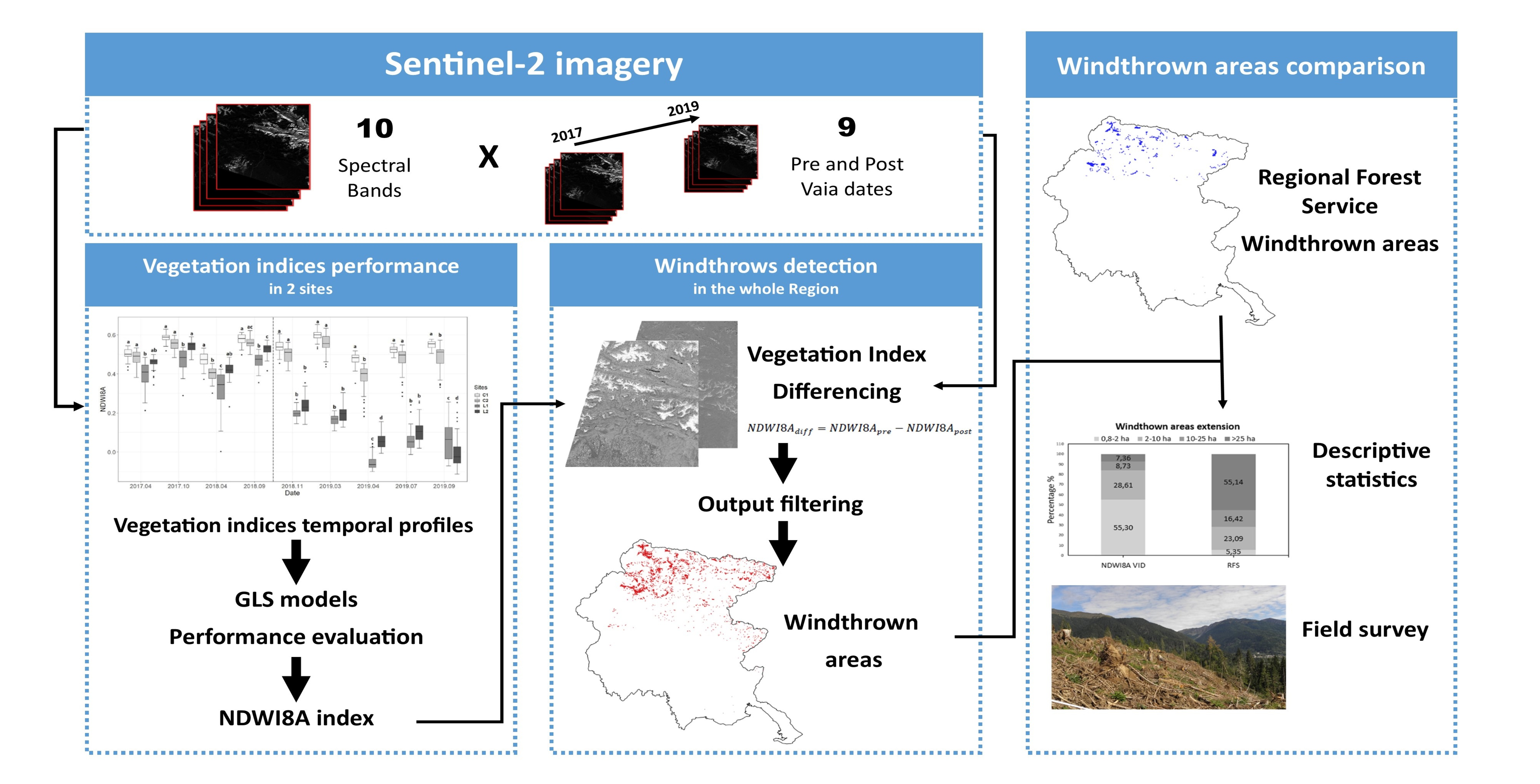
2. Materials and Methods
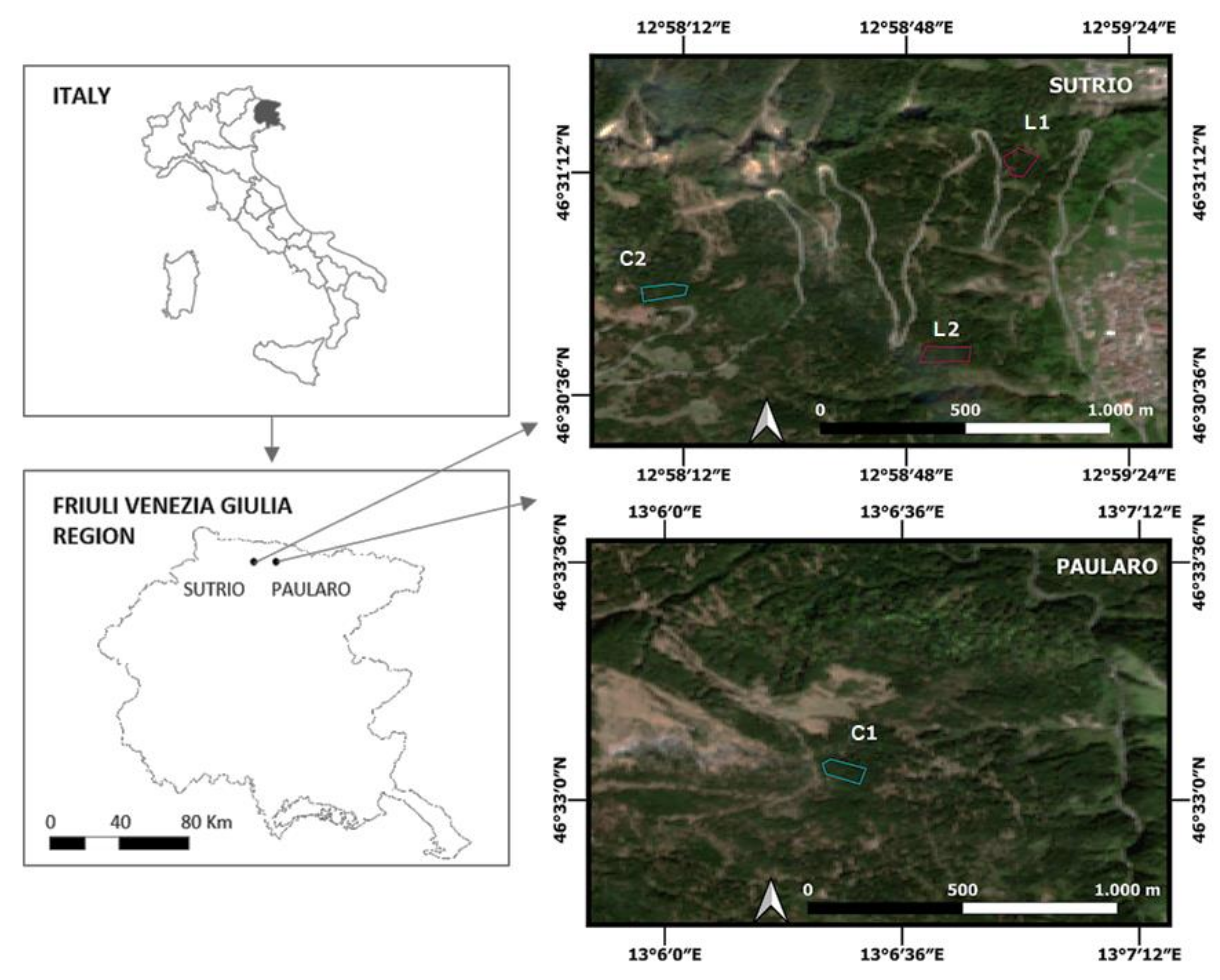
2.1. Study Sites

This study was performed in Carnic Alps, Friuli Venezia Giulia (Italy). The study area is located in Sutrio municipality, where large areal windthrow was recorded. The study site covers the south-eastern side of Zoncolan Mount (46°30′08″N, 12°55′34″E), and it is located in an area ranging in altitude from 750 m a.s.l. to 1250 m a.s.l. An additional site with the same S–E aspect has been chosen in Paularo municipality at 1250 m a.s.l. (46°31′51″N, 13°07′07″E). The climate is cold-temperate with mild summers and cold, but not particularly harsh, winters. Mean annual rainfall exceeds 2000 mm, mostly occurring in spring and autumn. In the study areas, winds are influenced by land morphology: valleys orientations, depth, width, aspect and solar radiation [17]. In this context, each mountain site differs in wind circulation characteristics even from geographically close areas. The synoptic winds triggered by storm Vaia reached 139 km/h gusts on Zoncolan summit, with mainly south-east and south-west mean direction [18]. The vegetation here was composed of coniferous forests dominated by Picea abies and Abies alba. Fagus sylvatica (L.) was also present but mixed with the previously mentioned main forest types.
The Vaia storm caused a heterogeneous damage pattern in Italian Eastern Alps temperate forests, resulting in scattered damaged areas with single and small groups of fallen trees or entire large areas with a uniform complete tree loss. Four sites, characterized by a pre-storm homogeneous vegetation cover of Picea abies and Abies alba have been selected (Figure 1): two were rather undamaged after Vaia, with an observed tree loss < 5%, and were referred to as control sites (C1 in Paularo, C2 in Sutrio), whereas L1, L2, both located in Sutrio municipality, had a uniform complete loss and were referred as windthrown sites. Each site covers a surface of approximately 1 ha, with a slope higher than 40% and south or east aspect. Slope, elevation and aspect maps were extracted from an 90 m resolution digital elevation model (DEM) processed using the “r.slope.aspect” function in GRASS 7.2 [19]. In “r.slope.aspect”, the aspect output raster map indicates the direction that slopes are facing counterclockwise from East: 90° is North, 180° is West, 270° is South, 360° is East. We then reclassified slope and aspect maps in 4 percentage classes as follows: 0–5%, 6–20%, 21–40% and > 40% for slope, N (45°–135°), E (0°–45° and ≥ 315°), S (225°–315°) and W (135°–225°) for aspect. The FVG 2017 Habitat Map [20] was used to select forest areas dominated by Picea abies and Abies alba. To avoid areas including deciduous species (i.e., Fagus sylvatica), pre-storm Sentinel-2 images acquired during the autumn season were used to visually check for the eventual presence of spots with colours typical of senescent leaves of deciduous species.

2.2. Remote Sensing Data

Sentinel-2 Level 2A (bottom of atmosphere) multispectral images with tile 33TUM were downloaded from Copernicus Open Access Hub [21] for the pre and post-Vaia dates showed in Table 1. Sentinel-2 images availability during late autumn and winter seasons was strongly reduced because of cloud cover, shadows, and snow presence. Accordingly, for the months immediately after the storm (from November to March), it was possible to retrieve only one image in November (15 November 2018) and one in March (5 March 2019).
In this study, 10 Sentinel-2 bands extend from the visible and near-infrared (VNIR) to the short-wave infrared (SWIR) were analysed in GRASS 7.2 [19], featuring:
  • four bands at 10 m: B02, blue (490 nm); B03, green (560 nm); B04, red (665 nm) and B08, near-infrared (NIR) (842 nm).
  • six bands at 20 m: B05–B07, three narrow bands in the vegetation red-edge (RE) spectral domain (705 nm, 740 nm, 783 nm); B8A, a narrow band in the near-infrared (NIR) (865 nm) and B11–B12, two large short-wave infrared (SWIR) bands (1610 nm and 2190 nm).
Bands values for each of the 4 study sites (L1, L2, C1 and C2) and for each of the 9 dates (2017.04, 2017.10, 2018.04, 2018.09, 2018.11, 2019.03, 2019.04, 2019.07, 2019.09) were extracted and eight vegetation indices (GNDVI, IRECI, NDREDI, NDVI, NDWI, NDWI8A, PSRI, SLAVI) were calculated using “r.mapcalc” function. Geographic boundaries for the sampling sites were set with the “g.region” and “r.mask” functions. The spatial resolution of the products is 10 m for GNDVI and NDVI. For the remaining indices, spatial resolution was set at 10 m by resampling lower resolution band pixels with the Nearest Neighbour algorithm with “r.resample” function in order to lose as little resolution as possible, considered the reduced extension of sampled sites. These indices take advantage of SWIR, NIR and RED, which have been proven highly effective in the detection of storm damages [22]. The indices used in this study are reported in Table 2.

2.3. Statistical Analyses

Pixel values for each multispectral index were plotted for each study site (L1, L2, C1 and C2) and each date through a boxplot using “ggplot2” R package [37]. In addition, each Sentinel-2 band (B02, B03, B04, B05, B06, B07, B08, B8A, B11 and B12) mean value and standard deviation for wind-damaged and control sites were plotted for each date to create spectral signatures. Generalize Least Square (GLS) models were used to test whether remote sensing indices were different between windthrown and control sites per each date, using gls function in “nlme” package [38]. Specifically, a GLS model was calculated for each remote sensing index (response variable) as a function of the study site type (fixed effect, 2 levels: control vs. windthrown). Temporal dependence among observations was incorporated through an autocorrelation structure of order 1. Model performance was evaluated computing the variance explained by the fixed effects using the function r2beta [39], with Nakagawa and Schielzeth method, available in R package “r2glmm” [40]. Differences between areas for the same date were assessed performing a GLS model for each index (response variable) as a function of area, date and their first order interaction using gls function, as described above. For significant models, posthoc pairwise comparisons were evaluated by “emmeans” R package [41]. Differences in band values for wind-damaged and control sites were assessed performing a GLS model for each band (response variable) as a function of site type, date and their first order interaction with gls function as described above. For significant models, posthoc pairwise comparisons of fixed effects interaction were evaluated as detailed above. Statistical analyses were performed using R 3.6.1 [42].

2.4. Change Detection

One of the most widely used mathematical operators to highlight image differences and detect changes is the image differencing method [43]. The method simply subtracts pre-image from post-image pixel values or vice versa. Despite the simplicity, image differencing methods have been widely used in previous studies devoted to wind-damage detection with considerable success [44,45,46]. In this study, the best VI identified by GLS models analysis (NDWI8A, see Results section) was employed in a (VID) technique in order to detect windthrown areas in whole Friuli Venezia Giulia Region Alpine forests. A new image called N D W I 8 A d i f f (20 m spatial resolution) was simply derived from the difference of NDWI8A raster values before Vaia and after Vaia:
N D W I 8 A d i f f = N D W I 8 A p r e N D W I 8 A p o s t
Summer and early autumn are recommended as the most suitable times for forest evaluation [22]. The 21st of April 2018 and the 21st of April 2019 were proven to be the best images for NDWI8A difference calculation as they were not affected by seasonal variations. Images acquired in different periods strongly differ by shadows presence and illumination on the ground. Moreover, the comparable period acquisition guarantees low phenological differences. The choice of spring season avoided the inconveniences related to the yearly variable water availability for forests at high altitudes. It has been observed that, at altitudes where snow is accumulated during winter (above approximatively 1500 m a.s.l.), the autumn vegetation water content, detected through the NDWI index, strongly depends on previous winter snow accumulation. However, albeit in a limited manner, spring images were not exempt from issues: most areas above 1500 m a.s.l. were still covered with snow in April, thus not included in the study. NDWI8Adiff values were masked using the Scene Classification Layers (SCL), retrieved in Sentinel-2 products, and the 2017 Regional Habitat Map [20]. In particular, NDWI8Apre was filtered for the SCL vegetation category while NDWI8Apost for both vegetation and not vegetated categories in order to include forest areas that turned not-vegetated because of the storm. NDWI8Adiff was then calculated from filtered images and further masked using the areas indicated as wooded in the 2017 Regional Habitat Map. Finally, NDWI8Adiff was filtered for values > 0.15, identified as the best threshold for windthrows detection, and converted from a raster product into a vectorial polygon. Finally, the obtained windthrown vectorial products were filtered for surfaces bigger than 800 m2 (2 pixels) in order to reduce the “noise” associated with scattered and spatially limited outputs.

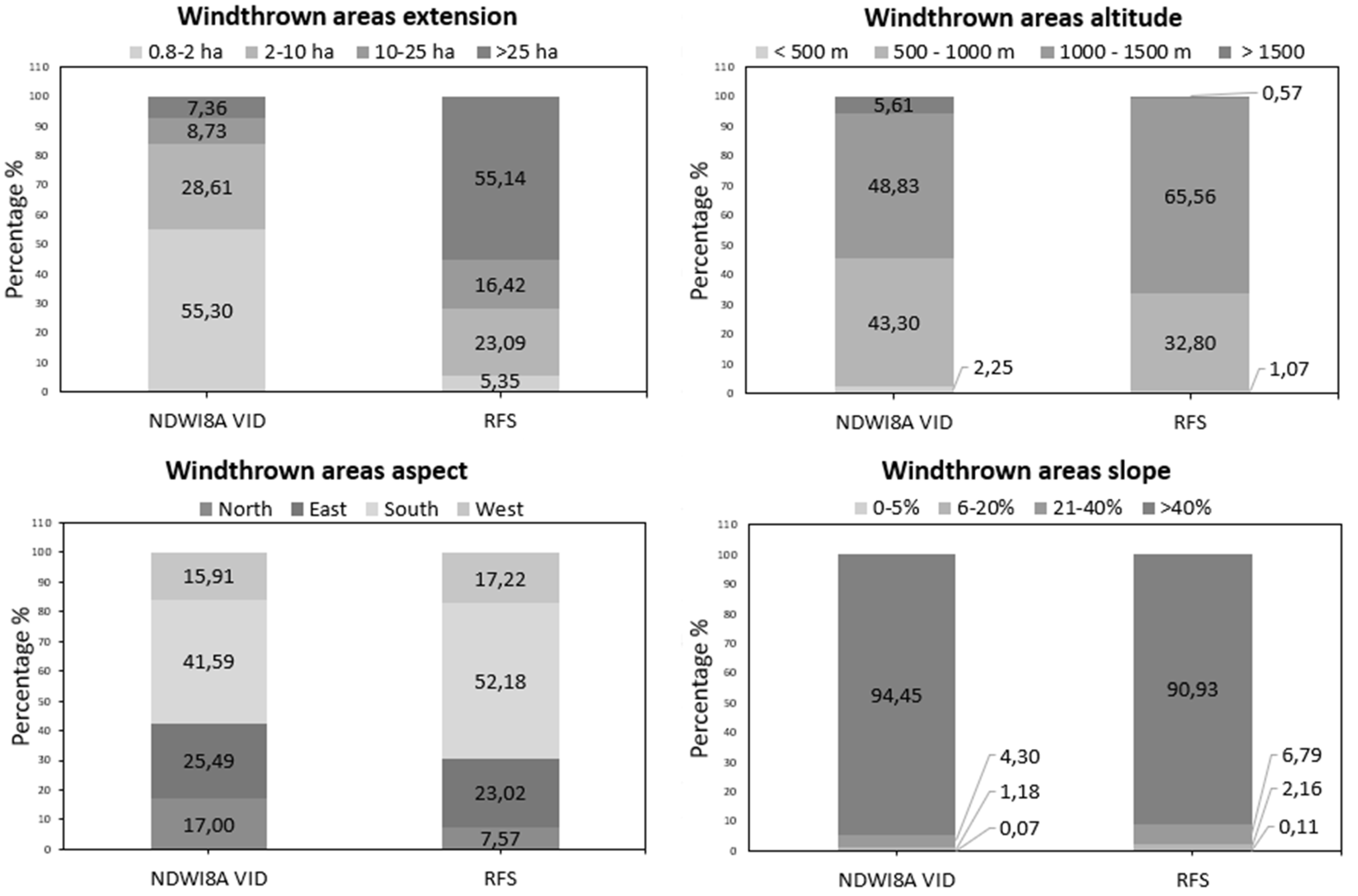
2.5. Descriptive Statistics on Regional Windthrows

Windthrows detected in Friuli Venezia Giulia Alpine forests with NDWI8A vegetation index differencing method were compared to reference Regional Forest Service (RFS) data. Descriptive statistics on the coverage of windthrown areas identified by the VID were extracted according to the elevation (4 classes: < 500 m, 500–1000 m, 1000–1500 m, >1500 m a.s.l.), aspect (4 classes: North, East, South, West), slope (4 classes: 0–5%, 6–20%, 21–40%, >40%) and extension (4 classes: 0.8–2 ha, 2–10 ha, 10–25 ha, > 25 ha) and compared to the ones extracted from the RFS windthrows perimeters. Moreover, GIS-provided geospatial data statistics were also used to assess the degree of similarity between the reference RFS data and the novel windthrows map obtained with the NDWI8A VID method in RFS perimeters. Statistics on damaged forests by municipality for both NDWI8A VID and RFS were extracted and the % error of NDWI8A VID method with respect to RFS estimations was calculated as:
N D W I 8 A V I D   % e r r o r = N D W I 8 A V I D a r e a R F S a r e a N D W I 8 A V I D a r e a + R F S a r e a 100

2.6. Map Validation

A reference map of Vaia windstorm impacts was generated based on field survey data provided by the Regional Forest System (RFS). The fieldwork took place in all Friuli Venezia Giulia Region after Vaia storm. Although the accuracy of this data is limited by surveyors’ possibility to access and spot damaged areas, the RFS reference map provides a comprehensive collection of available data of Vaia-caused disturbance in forests across a large portion of the Regional territory, thus providing a useful tool for comparison with remote sensing data. For both RFS and NDWI8A VID maps, validation was obtained by field assessment along the valley of Tagliamento river, where, according to the reference material, most damages occurred. Field survey observations were substantiated by georeferenced pictures, which offered a descriptive insight into Vaia disturbances impacts, also providing a qualitative check of windthrow maps.

3. Results

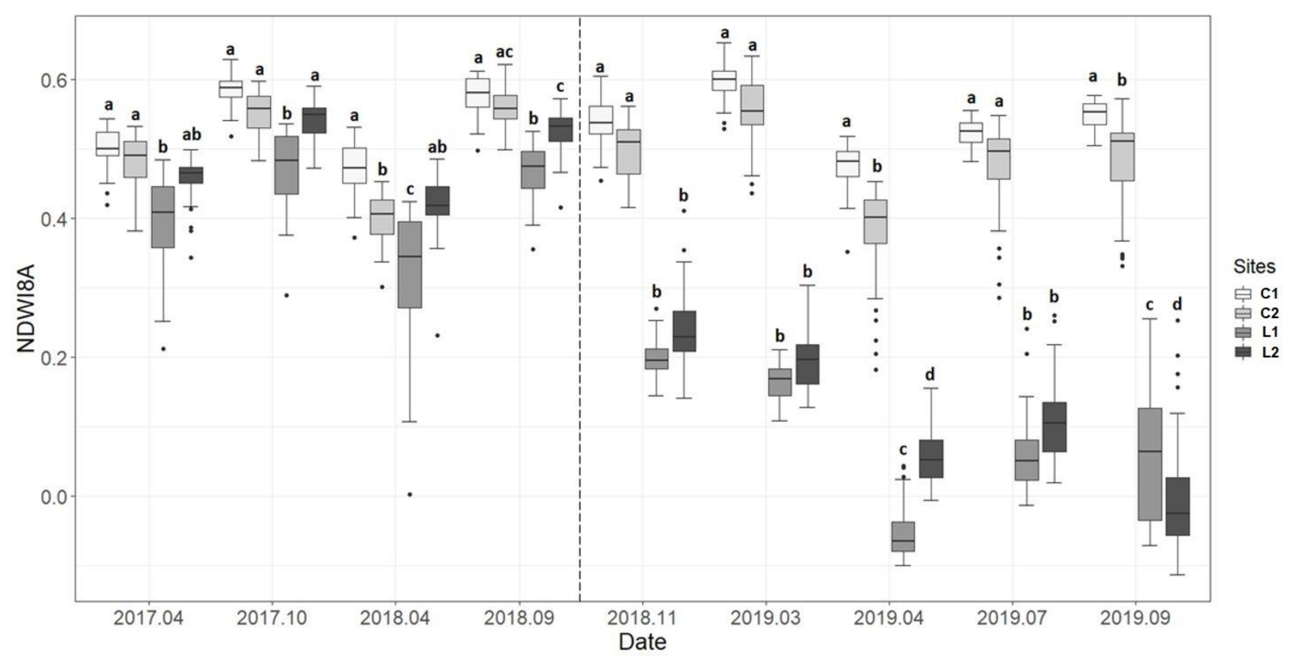
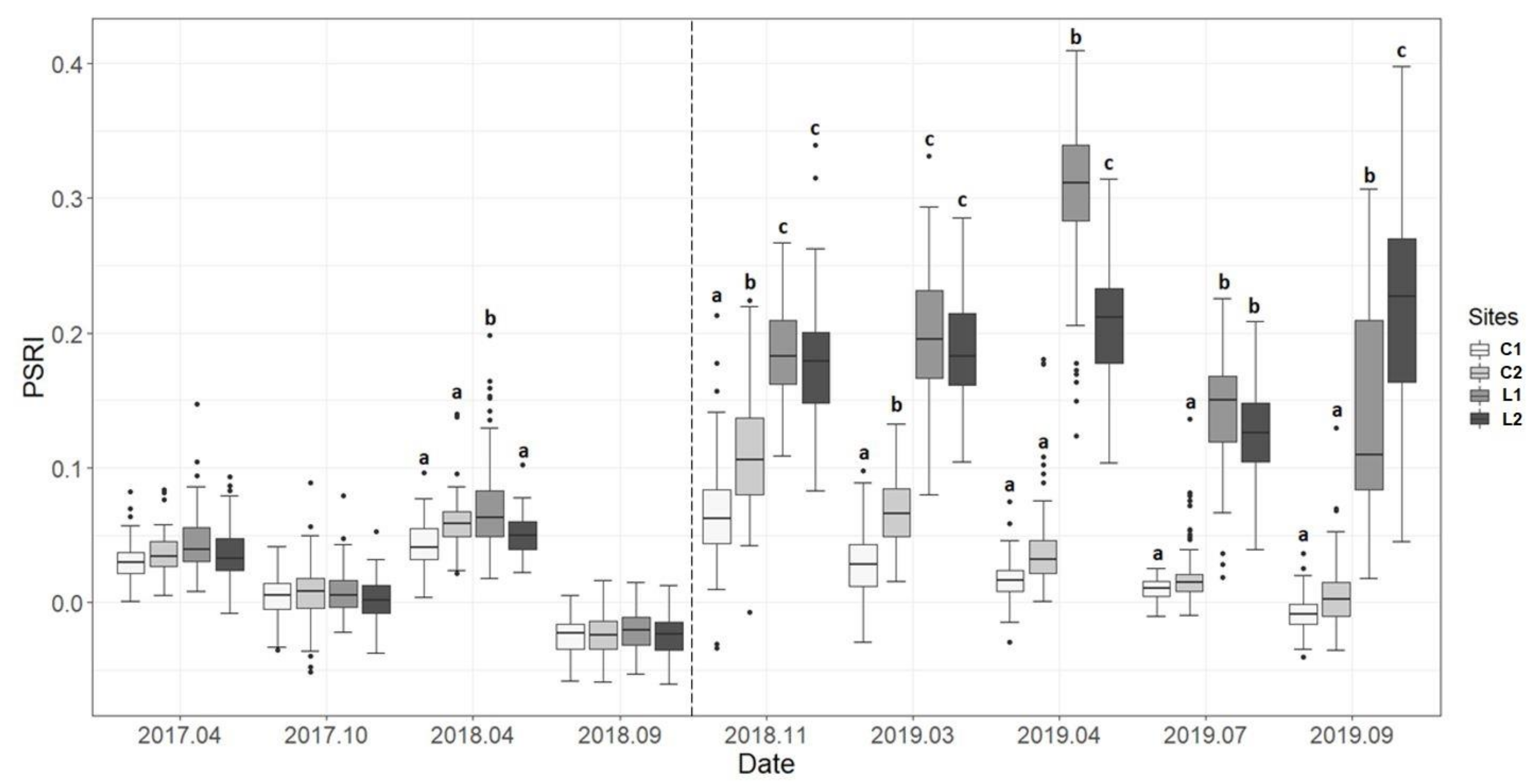
3.1. Temporal Profiles of Vegetation Indices

Boxplot of temporal profiles of the NDWI8A and PSRI indices both for windthrown and control study sites showed that indices values after Vaia in L1 and L2 windthrown sites are significantly lower for NDWI8A and higher for PSRI than in C1 and C2 control sites, differently, being almost comparable before Vaia (Figure 2 and Figure 3). The remaining indices temporal profiles are shown in Supplementary Materials (Figures S1–S6). GLS model outputs for each index as a function of area, date and their interaction are shown in Supplementary Materials (Table S1). For each of the eight indices considered in this study (except IRECI and NDREDI), the values of the indices remained quite constant in control sites during all the period of investigation, taking into account seasonal variations. In NDVI, NDWI, NDWI8A, SLAVI, GNDVI, IRECI indices, L1 and L2 sites pixel values were comparable to control sites before the Vaia event, but they showed significantly lower values after it. Notably, the PSRI index showed an inverse pattern compared to the other indices. The index NDREDI showed differences between controls and windthrown sites on the first date after Vaia (2018.11), having comparable values in windthrown and control sites in the remaining dates (Figure S6). An increase in control sites’ variability was detected after Vaia for all indices, less evidently in NDWI8A compared to other indices.

3.2. Vegetation Indices Performance

Table 3 showed GLS model outputs; NDWI8A was the best index for windthrows detection accounting for 80% of variance explained (see R2 in Table 3). NDWI, NDVI, PSRI, SAVI and GNDVI had an overall good performance in spotting wind damages (spanning from 0.60 to 0.77 of R2). For IRECI the effect of the treatment explained 32% of data variability, while for NDREDI just 3%. In contrast, PSRI showed a significant decrease after the Vaia storm compared to the previous period.

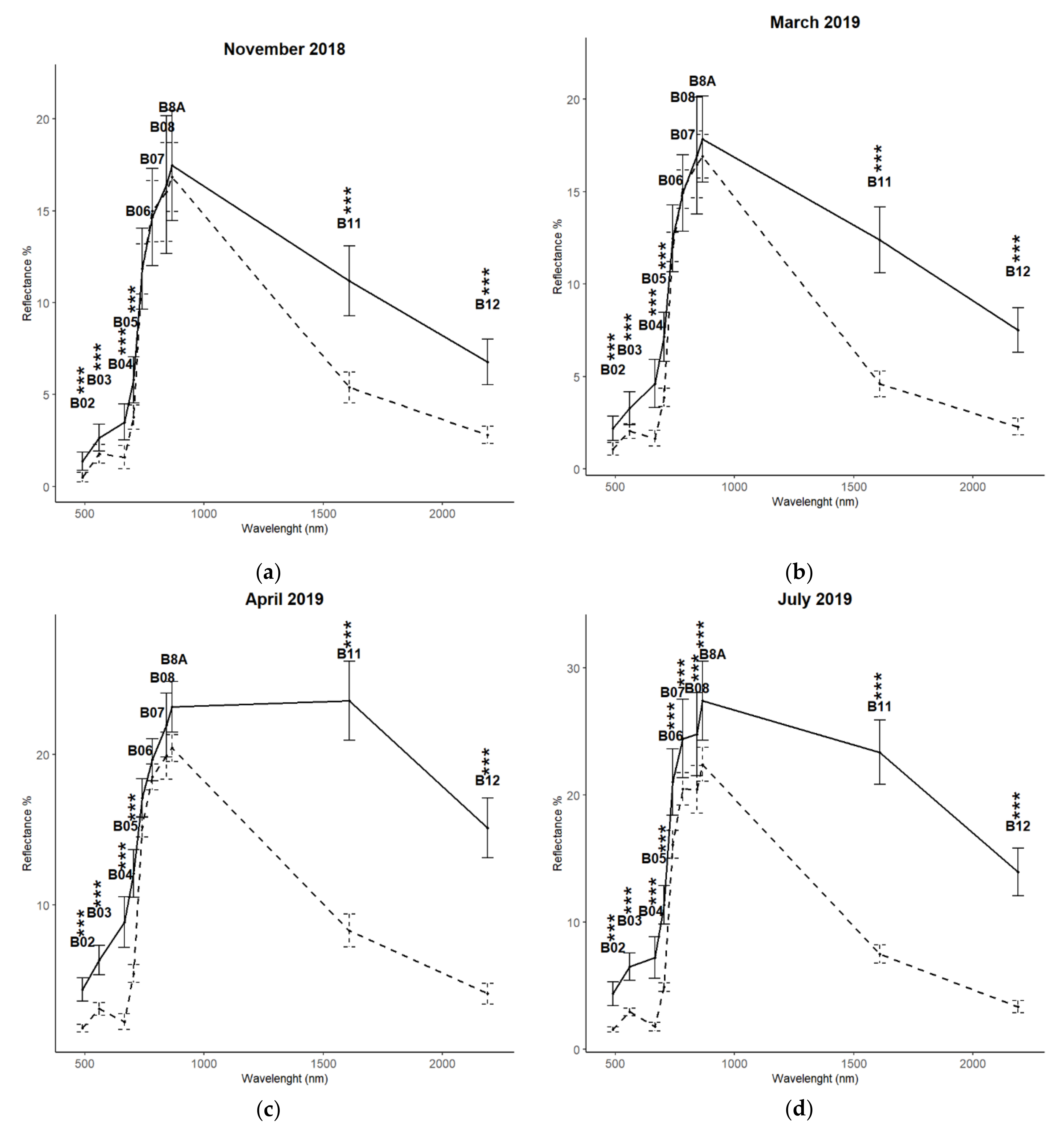
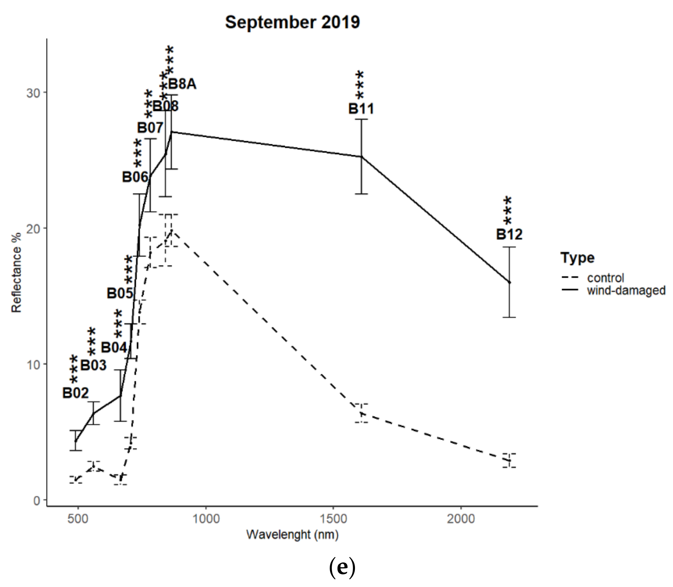
3.3. Spectral Signatures

Controls and Wind-damaged sites spectral signatures for each date after the Vaia event are shown in Figure 4. GLS models’ outputs for each band are shown in Supplementary Materials (Table S2). Band positions on the wavelength spectrum along with their significance are also shown. Band central wavelengths are: B02–490 nm, B03–560 nm, B04–665 nm, B05–705 nm, B06–740 nm, B07–783 nm, B08–842 nm, B8A–865 nm, B11–1610 nm, B12–2190 nm.
In November 2018, control and wind-damaged signatures followed a very similar pattern. Indeed, both showed two absorption peaks on blue and red regions (B02 and B04, respectively), an increasing reflectance from red to near-infrared (NIR) (from B04 to B8A) and lower reflectance values in the short-wave infrared (SWIR) region (B11 and B12). Control and wind-damaged signatures overlapped from red-edge to NIR (from B06 to B8A), but wind-damaged sites had significantly higher reflectance in the remaining bands. Control sites mean reflectance in the visible (form B02 to B04) spanned from 0.5% to 0.8%, in contrasts, damaged sites reflectance ranged between 1.3% to 3.5%. The reflectance of the first band of red-edge (B05) was higher in wind-damaged sites (5.8%), rather than in controls (3.8%). Differently from wind-damaged sites, controls had an evident absorption in the SWIR region. Accordingly, SWIR1 and SWIR2 reflectance was 11.2% and 6.8% in wind-damaged sites and 5.4% and 2.8% in controls.
In March and April windthrown sites spectral signatures, we observed increasing reflectance values in the B04 red band and in B11 and B12 SWIR ones. In March B04, B11 and B12 reflectance in windthrown sites (4.6%, 12.4% and 7.5%) was almost 3 times higher than controls reflectance (1.7%, 4.6%, 2.3%). In April, B04 and B12 reflectance in wind-damaged sites was 4 times that of the control. In April 2019, the highest reflectance for wind-damaged sites was registered in the SWIR region (B11, 23.5%) rather than in the NIR (B8A, 23,1%). Moreover, in wind-damaged site signatures, the absorption peak in the red was no more visible as reflectance grew linearly from B02 to B04. In the same period a slight increase in the signatures distance between the red-edge and the NIR overlapping region was observed; in April 2019, B05, B06, B07, B08, B8A mean reflectance in windthrown sites (12.1%, 17.1%, 19.6%, 21.9%, 23.1%) was higher than controls one (5.4%, 15.2%, 18.5%, 20%, 20.4%).
From July 2019, a significantly higher reflectance between the red-edge and NIR region (B05–B8A) was also registered in wind-damaged sites rather than in controls. In September 2019, the gap between the two signatures in the NIR had a further growth; B8 and B8A reflectance was 25.3% and 16% in wind-damaged sites and 6.4% and 2.9% in controls. In July and September 2019, a slight absorption in the red region reappeared, as an inflection point is visible in B03.

3.4. NDWI8A VID Windthrow Map

The output obtained through NDWI8A vegetation index differencing indicated a wind-damaged area of 2545 ha. The Regional Forest Service estimation, obtained through manual digitalized perimeters, indicated damage of 3183 ha. Figure 5 shows windthrown area coverage statistics, for both NDWI8A VID and RFS estimations, extracted according to the extension, elevation, aspect and slope.
For both methods, wind-damaged areas were arranged in comparable classes of elevation. According to NDWI8A VID and RFS methods, the highest damage was detected from 1000 to 1500 m a.s.l. (49% and 66%, respectively), followed by 500–1000 m a.s.l. (33% for NDWI8A VID and 43% for RFS). Interestingly, at higher elevations (>1500 m a.s.l), NDWI8A VID detected higher damage compared to RFS (6% vs. 0.57%, respectively). Both NDWI8A VID and RFS methods had similar classes of slope aspects. However, the NDWI8A VID method had higher damage in north exposed slopes detrimental to south ones, when compared to RFS. Most damages were registered in the south (42% for NDWI8A VID, 52% for RFS) and east slopes (25% and 23%, respectively). For slope, again, damaged areas identified by the two methods are arranged in comparable percentual classes. More than 90% of the damage was detected in areas whose inclination is bigger than 40%. Finally, the methods showed discrepancies in classes of damages extension. According to the NDWI8A VID method half of the damaged surface is made up of a multitude of small areas (0.8–2 ha). On the contrary, RFS detected half of the damage in large areas (bigger than 25 ha).
Of the total 2545 ha delimited areas of NDWI8A VID, 661 ha were included in RFS estimations (26%), while the remaining 1884 ha (74%) fell outside from RFS perimeters. NDWI8A VID % error with respect to RFS estimations was 65.60%. Table S3 reports NDWI8A VID and RFS estimations in RFS delimited areas and NDWI8A VID % error as compared to RFS estimations for each municipality.

3.5. Map Validation

The Friuli Venezia Giulia windthrown areas, obtained through the NDWI8A VID technique, were visually compared to the ones provided by the Regional Forest Service (RFS) and overall accuracy was assessed by field surveys. The field survey was conducted on the 1st of February 2020 in Tagliamento Valley, in the municipalities of Villa Santina, Ampezzo and Forni di Sotto, where most damages were registered according to RFS. As shown by field surveys pictures available in Supplementary Materials (Figure S7), the VID method successfully delimited areal windthrows, being in most cases more precise than foresters’ estimation and able to identify areas that were not included in RFS perimeters.

4. Discussion

4.1. Vegetation Indices Temporal Profiles

In our study, NDWI and NDWI8A were identified as the best indices to separate wind-damaged from undamaged sites, suggesting windthrow-induced water stress (R2 = 0.80 and 0.77, respectively). Windthrow inevitably disrupted the soil–plant–atmosphere water continuum, decoupling the root system from soil or interrupting water movement through the xylem by damages at stem level [47]. The catastrophic failure of the water transport system led to water deficit in damaged plants immediately after the Vaia storm, and it was successfully detected using NDWI and NDWI8A indices right after the storm, through the abrupt rise of SWIR reflectance (Figure S1, Figure 2). Moreover, for most plants, canopy water content could not have recovered to control levels, as SWIR reflectance did not change in the following 11 months (Figure 4). This suggests that Vaia-event could have triggered extensive branch desiccation or, in the worst cases, tree mortality (forest die-off), as windthrows likely negatively affected the canopy water content both in the immediate and in the long-term period. This hypothesis is furtherly confirmed by the lower values of NDVI, which is highly correlated to plant productivity and vitality [44], calculated in damaged sites after the storm, Plant water status can be estimated by several physiological parameters, such as: (1) leaf water potential (i.e., water-free energy in plant organs), (2) leaf water content (usually expressed as the volume of water in leaves relative to the fully hydrated status) and (3) equivalent water thickness (EWT, i.e., the total water mass in the foliage per ground surface area) [48,49]. According to Hunt Jr et al. [50], EWT can be estimated by spectral reflectance at shortwave-infrared (SWIR) wavelengths, which are sensitive to water content. Moreover, indices calculated from a normalized difference of NIR and SWIR bands, such as NDWI, were found to be strongly related to canopy EWT using various sensors such as: Landsat TM, ASTER, AWiFS and SPOT [48,51]. Recently, Marusig et al. [52] found strong correlations between both midday leaf water potential and leaf water content and Sentinel-2 derived NDWI. Finally, special attention should be paid to NDWI8A which, despite the relatively low spatial resolution of 20 m, was the best index for this study purpose. This result confirms the usefulness of the narrow B8A at 865 nm in the NIR, designed to avoid contamination from water vapour through a high spectral resolution and yet successfully being able to represent the NIR plateau for vegetation.
Despite computing shorter wavelength bands (B8 and B4), the NDVI index successfully detected windthrows events (Table 3: R2 = 0.76), as previously shown in other studies [26,45,53]. NDVI is the most consolidated index used to study the spectral behaviour of vegetation and it has been widely used as a proxy for green biomass and plant productivity [28,44]. The increase in reflectance registered in the red and blue regions (B02 and B04) in wind-damaged sites (Figure 4) suggests that windthrow inevitably affected also plants photosynthetic efficiency. Usually, under water-limited conditions, plants tend to prevent water loss by decreasing stomatal aperture (or by complete stomatal closure), which in turn also causes a decrease in the photosynthetic rates and allows plants to avoid excessive photosynthetic pigments excitation [54]. In our case, windthrow-induced water transport interruption triggered plant mortality thus affecting the photosynthetic activity from the outset. GNDVI was less efficient than NDVI in separating wind-damaged from undamaged classes (Table 3: R2 = 0.60). The GNDVI was suggested to avoid the NDVI saturation effect in dense canopy structures and it uses the green band (B3) as a replacement for the red one (B04) [24]. However, the use of B03 rather than B04 has lowered GNDVI sensitivity to Vaia-induced changes in forests’ photosynthetic efficiency.
In this sense, an interesting output is shown by PSRI performance in separating wind-damaged and control sites (Table 3: R2 = 0.69). This index is sensitive to photosynthetic pigments relative content (both chlorophyll and carotenoids) and it has been widely used as a quantitative measure of leaf senescence [55,56]. When a plant starts dying, canopy discoloration occurs and immediate reduction in chlorophyll rather than in carotenoid concentrations decreases the spectral absorbance in the red region [33]. Moreover, reflectance in the red region increases significantly due to the production of anthocyanins, triggered by water stress [57]. The increase of reflectance in the red region rather than in the blue one proved that PSRI could be successfully used to monitor tree vitality and to determine the onset of wind-induced mortality. This also explains the index inverse pattern with respect to all the other indices, in PSRI low values were found in control sites while high values were associated with wind-damaged ones (Figure 3).
Despite it computes B12 band, which should correlate to changes in canopy water content, the SLAVI index was not as effective as NDWI and NDWI8A in detecting windthrows (Table 3: R2 = 0.65). It is probable that the sum of red and SWIR bands, a proxy for photosynthetic efficiency and water content respectively, has increased the sensibility of the index in healthy forests. High seasonal fluctuations in SLAVI temporal profiles were registered in control values rather than wind-damaged sites, which maintain very low values (Figure S3). NIR reflectance provides information about the cell structure of the plant and is widely used in vegetation monitoring [28]. However, in contrast with outputs in Einzmann [26], NIR reflectance did not change immediately after Vaia, indicating that the leaf structure of the damaged trees was not affected by the storm (Figure 4). This might be due to the fact that conifers usually occupy the conservative region of the Leaf Economic Spectrum (LES) [58], having higher LMA (leaf mass per area), greater lamina thickness, content of mechanical tissues, and thickness and sclerification of mesophyll cell walls [59], which guarantee longer leaf lifespan, with respect to broadleaves. Thus, the immediate post-storm period is likely excessively early to detect any leaves’ structural deterioration. Besides the NIR, B06 and B07 red-edge bands of post-storm images were also not important for windthrow characterization (Figure 4). An exception is applied for the B05 band, whose values were significantly higher immediately after Vaia, thanks to its close relationship to the red region rather than NIR. In our study, IRECI and NDREDI, both using red-edge bands, were the least effective indices for wind-damage detection (Table 3). The model including IRECI explained the 32% of data variance while regarding NDREDI, the model explained a minimal part of data variance (3%), proving to be incapable of discriminating damaged from undamaged stands. These results collide with those in Einzmann [26], where the red-edge was indicated as the most important channel for windthrow identification. These differences could be due to the fact that damaged sites in Einzamann [26] might have a higher proportion of deciduous species (e.g., Fagus sylvatica), or to the different season when the storm occurred (March for Storm Niklas while October for Vaia), and not least the different pixel resolution (5 and 10 m in Einzmann vs. our study, respectively). In this study, PSRI was the only index that includes a RE band to be suitable for the detection of stressed or damaged vegetation. However, as already mentioned, its suitability for windthrows detection was mainly attributed to changes in blue and red regions reflectance rather than in RE.
Together, spectral signatures (Figure 4) and LMMs outputs (Table 3) showed that visible (B02, B03, B04), the first RE (B05) and short-wave infrared (B11, B12) were the most important bands to detect windthrows, as their values differed between damaged and un-damaged sites, even immediately after the storm. On the other hand, remaining RE (B6, B7) and NIR (B8 and B8A) band values did not differ between damaged and un-damaged sites. Indices which include one or more of these variable bands (B02, B03, B04, B05, B11, B12), together with one band which do not change from damage to un-damaged classes (B6, B7, B8, B8A), so-called “invariant”, have been proved to be successful in identifying damaged sites. Similar results were recently obtained by Stych et al. [22], as they concluded that indices that take advantage of red, NIR and SWIR bands are the most sensitive and effective for the detection of wind disturbances in forests.

4.2. Spectral Reflectance of Vegetation after Windthrow

NIR reflectance did not vary between windthrown and control sites immediately after Vaia hit. A significant increase of B8 and B8A values in wind-damaged sites spectral signatures was registered 6 months after the storm, which corresponded to the resumption of the forest vegetative cycle (Figure 4). In the field of remote sensing of vegetation, it is common knowledge that NIR reflectance is generally lower for conifer crowns than broadleaf crowns due to different structural features which affect light scattering [60,61,62,63]. In view of the increase of reflectance in the NIR registered in spring (Figure 4), we suggest that windthrown sites may have undergone a secondary succession process. Consequently, this process might have caused a rapid recolonization of grasses and other herbaceous plants, several shrubs and many rapid-growing pioneer species. This recolonization has been facilitated by the tree removal which occurred in L1 (first two weeks of April 2019) and L2 (August 2019) batches. This was particularly evident in site L1, which was the first area subjected to batch cleaning. On 24 September 2019, the inspection in site L1 revealed that many typical light-requiring species were present in post-disturbance sites (e.g., Carex spp., Sambucus spp., Rubus ideaus, Pteridium aquilinum, Salvia glutinosa), as well as large populations of regenerating trees (e.g., Castanea sativa, Corylus avellana). This gradual colonization matches with the increased variability of all vegetation indices values except NDREDI, registered in site L1 on the 13rd of September 2019 (Figure 2 and Figure 3, Figures S1–S5). The increase in index variability post-Vaia in C1 and C2 sites suggests that partial damage in these sites may have occurred (Figure 2 and Figure 3, Figures S1–S6). It is probable that both control sites have been subjected to scattered windthrows, considering that their location, vegetation composition, lithology, slope, aspect and elevation is comparable to windthrown sites. These limited damages have been confirmed in the C2 site through the field survey; many scattered trunks and branches were present on the site forest floor. Interestingly, all vegetation indices except NDREDI also caught L1 and L2 batches tree removal; L1 values were almost comparable to L2 in March 2019, lower in April 2019, while L2 had lower values in September 2019 rather than in July 2019, when compared to L1 (Figure 2 and Figure 3, Figures S1–S5).

4.3. NDWI8A VID Windthrow Maps

The NDWI8A differencing method successfully detected 2545 ha of forests affected by wind-caused damages, differently from The Regional Forest Service estimation, which indicated damage of 3183 ha. Of the 2545 ha NDWI8A VID delimited areas, 661 ha were included in RFS estimations, corresponding to a 65.60% error (Table S3). It is possible that manually digitalized perimeters have overestimated effectively windthrown areas for practical reasons. First, the Vaia storm did not impact forests uniformly within each RFS polygon. As qualitatively shown during field inspections, RFS included large forest patches that suffered from very scattered damage rather than intense areal damage. Secondly, the proposed method is not suitable for widespread damage as it requires intense and rather uniform damage to satisfy NDWI8A and extension thresholds. These considerations also explain the overall smaller wind-damaged area detected by the NDWI8A vegetation index differencing method than the one offered by the Regional Forest Service (Figure 5). Windthrown area extension classes differ in the two methods: half of the areas detected by our method are small (0.8–2 ha) whereas the same quantity in RFS is represented by the biggest class (>25 ha). This difference may arise from the difficult conditions of the ground survey in RFS data, due to hard-to-access terrain and remote location of small disturbances. In fact, most areas are hardly accessible and located in remote and steep areas where field inspections and accurate manual perimeters may have been impossible to carry out. In this context, foresters may have preferred a wide perimeter strategy to include all possible damaged areas. On the other hand, according to Figure 5, the damage pattern highlighted following our method was similar to the one described by the RFS, particularly in relation to elevation, aspect and slope characteristics. The elevation, the high slope, and south/east main aspects of the windthrown areas match the Vaia storm evolution and interaction with the mountainous landscape of Friuli Venezia Giulia Alps and pre-Alpes. The Vaia scirocco gusts were channelled in the Alpine valleys causing most damages in the forests along steep mountain slopes where compression forces were amplified [11].
From an ecological perspective, the Vaia storm caused windthrows to many tree species such as Picea abies, Abies alba, Fagus sylvatica and species belonging to Alnus and Salix genera. Interestingly, many species considered as wind-resistant, such as beech, were subjected to windthrow suggesting that gusts’ extreme speeds have by far exceeded plant-specific resistance. The vulnerability of Alnus and Salix sp. could have increased due to their exposed position and the presence of soils nearby the river expansion, whose humidity might have been increased by the strong precipitations associated with the Vaia storm.

4.4. Study Limitations

In this study, the NDWI8A vegetation index differencing method did not provide a prompt post-storm windthrow map to be used for Vaia impact assessment, as images acquired shortly after this extreme event were having a too low quality to be used as input. This is indeed the limitation of using optical remote sensing in winter storm-associated disturbances studies. Sentinel-2 data use has been strongly limited by shadows and snow presence, as well as cloud cover that occurred in the weeks near to the event [12]. However, as qualitatively shown by our field inspections, the NDWI8A differencing method provides satisfying and reliable windthrow maps. At last, most of the detected areas have intense and uniform damage which was not found in RFS large perimeters. The proposed method may offer a more accurate and easy way to delimit windthrows damages in the forests. Nevertheless, proper validation is still missing. Visual assessment and field surveys offer a broad screening that cannot be used for proper accuracy assessment. In the future, the accuracy assessment of NDWI8A VID-derived windthrow maps should be provided by extensive ground truth data. These data may be accurate forest use notifications data (which report possible occurred wind-damages), forest-stand updated datasets or high-resolution remote sensing data, such as Light detection and ranging (LiDAR) or orthophotos. Moreover, since clear-cutting and phenology effects can bring uncertainties, future studies should pay attention to choosing images for the proposed method. It should be recalled that VID chosen images were taken far away from the date on which the natural phenomena occurred when forests optimal sensing is guaranteed. The early spring period rather than autumn should be favoured when cleaning activities have not started yet.

5. Conclusions

Vegetation indices that highlight damaged-areas differences in the visible and the SWIR regions are strongly recommended for the detection of windthrows and for the monitoring of both forest die-off and succession dynamics. NDWI8A VID is an easy and cost-effective method able to produce reliable windthrow maps. Our results showed that the proposed method successfully delimited areal windthrows caused by the Vaia storm in forests throughout the Friuli Venezia Giulia Region. This study provides a safer alternative to detect the location of damaged areas, avoiding the risks associated with field inspections, especially in hardly accessible steep areas. Finally, the obtained results could be helpful in identifying sensitive areas to potentially uncontrollable insect/pathogen outbreaks. Such areas are advisable for sanitation as a preventive intervention to remove potential attractive host material for tree bark beetles and other pathogens [64].

Supplementary Materials

The following supplementary materials are available online at https://0-www-mdpi-com.brum.beds.ac.uk/article/10.3390/rs13081530/s1. Figure S1: NDWI, Figure S2: NDVI, Figure S3: SLAVI, Figure S4: GNDVI, Figure S5: IRECI, Figure S6: NDREDI, Figure S7: Field survey areas, Table S1: Outputs of Generalized Least Square models for indices, Table S2: Outputs of Generalized Least Square models for Sentienl-2 bands, Table S3: Comparison of NDWI8A VID and RFS estimations for municipality.

Author Contributions

Conceptualization, A.A., V.O.; Data curation, V.O.; Formal analysis, V.O., E.T., F.P.; Writing—original draft, V.O., A.A.; Writing—review & editing, G.B., E.T., F.P. All authors gave final approval for publication. All authors have read and agreed to the published version of the manuscript.

Funding

This research received no external funding.

Institutional Review Board Statement

Not applicable.

Informed Consent Statement

Not applicable.

Data Availability Statement

Sentinel-2 data presented in this study are openly available at Copernicus Open Access Hub https://scihub.copernicus.eu/ (accessed on 30 September 2019). The digital elevation model (DEM) of Friuli Venezia Region is available at: https://srtm.csi.cgiar.org/srtmdata (accessed on 19 August 2019). Windthrows areas delimited by the Friuli Venezia Giulia Region Forest Service are available upon request.

Acknowledgments

We would like to thank Daniel Marusig for helping and supporting the first fundamental steps of the research conceptualization and methodology and Massimo Zia for help with data recovery.

Conflicts of Interest

The authors declare no conflict of interest. The funders had no role in the design of the study; in the collection, analyses, or interpretation of data; in the writing of the manuscript, or in the decision to publish the results.

References

  1. Dash, J.P.; Watt, M.S.; Bhandari, S.; Watt, P. Characterising Forest Structure Using Combinations of Airborne Laser Scanning Data, RapidEye Satellite Imagery and Environmental Variables. Forestry 2016, 89, 159–169. [Google Scholar] [CrossRef] [Green Version]
  2. Van Westen, C.J. Remote Sensing and GIS for Natural Hazards Assessment and Disaster Risk Management. In Treatise on Geomorphology; Elsevier: New York, NY, USA, 2013; pp. 259–298. ISBN 978-0-08-088522-3. [Google Scholar]
  3. I.P.C.C. Summary for Policymakers. In Climate Change and Land: An IPCC Special Report on Climate Change, Desertification, Land Degradation, Sustainable Land Management, Food Security, and Greenhouse Gas Fluxes in Terrestrial Ecosystems; IPCC/IGES: Hayama, Japan, 2019. [Google Scholar]
  4. Gardiner, B.; Schuck, A.R.T.; Schelhaas, M.J.; Orazio, C.; Blennow, K.; Nicoll, B. Living with Storm Damage to Forests: What Science Can Tell Us; European Forest Institute: Joensuu, Finland, 2013; Volume 3, pp. 1–132. [Google Scholar]
  5. Schuck, A.; Schelhaas, M.J. Storm damage in Europe–An overview. In Living with Storm Damage to Forests: What Science Can Tell Us; Gardiner, B., Schuck, A.R.T., Schelhaas, M.J., Orazio, C., Blennow, K., Eds.; European Forest Institute: Joensuu, Finland, 2013; Volume 3, pp. 15–24. [Google Scholar]
  6. Anderegg, W.R.; Kane, J.M.; Anderegg, L.D. Consequences of Widespread Tree Mortality Triggered by Drought and Temperature Stress. Nat. Clim. Change 2013, 3, 30–36. [Google Scholar] [CrossRef]
  7. Nowacki, G.J. The Effects of Wind Disturbance on Temperate Rain Forest Structure and Dynamics of Southeast Alaska; US Department of Agriculture, Forest Service: Portland, OR, USA, 1998; Volume 421.
  8. Sinton, D.S.; Jones, J.A.; Ohmann, J.L.; Swanson, F.J. Windthrow Disturbance, Forest Composition, and Structure in the Bull Run Basin, Oregon. Ecology 2000, 81, 2539–2556. [Google Scholar] [CrossRef]
  9. Peltola, H.; Gardiner, B.; Nicoll, B. Mechanics of wind damage. In Living with Storm Damage to Forests: What Science Can Tell Us; Gardiner, B., Schuck, A.R.T., Schelhaas, M.J., Orazio, C., Blennow, K., Eds.; European Forest Institute: Joensuu, Finland, 2013; Volume 3, pp. 31–38. [Google Scholar]
  10. Mitchell, S.J.; Ruel, J.-C. Modeling Windthrow at Stand and Landscape Scales. In Simulation Modeling of Forest Landscape Disturbances; Perera, A.H., Sturtevant, B.R., Buse, L.J., Eds.; Springer International Publishing: Cham, Switzerland, 2015; pp. 17–43. ISBN 978-3-319-19808-8. [Google Scholar]
  11. Carraro, V. La Furia del Vento che ha Danneggiato le Foreste dell’arco Alpino; Centro Studi per L’ambiente Alpino L: Cadore, Italy, 2019. [Google Scholar]
  12. Chirici, G.; Giannetti, F.; Travaglini, D.; Nocentini, S.; Francini, S.; D’Amico, G.; Calvo, E.; Fasolini, D.; Broll, M.; Maistrelli, F.; et al. Forest damage inventory after the “Vaia” storm in Italy. Forest 2019, 16, 3–9. [Google Scholar] [CrossRef] [Green Version]
  13. Directorate Space, Security and Migration, European Commission Joint Research Centre (EC JRC). Copernicus Emergency Management Service. Available online: https://emergency.copernicus.eu/ (accessed on 17 October 2019).
  14. Chang, J.; Ciais, P.; Herrero, M.; Havlik, P.; Campioli, M. Combining Livestock Production Information in a Process-Based Vegetation Model to Reconstruct the History of Grassland Management. Biogeosci. Eur. Geosci. Union 2016, 3757, 3757–3776. [Google Scholar] [CrossRef] [Green Version]
  15. Xue, J.; Su, B. Significant Remote Sensing Vegetation Indices: A Review of Developments and Applications. J. Sens. 2017, 2017, 1–17. [Google Scholar] [CrossRef] [Green Version]
  16. Copernicus Emergency Management Service EMSR334: Wind Storm in North-East of Italy. Available online: https://emergency.copernicus.eu/mapping/list-of-components/EMSR334 (accessed on 11 November 2019).
  17. Osmer, O. Metereologico regionale del FVG. In Il Clima del Friuli-Venezia Giulia; ARPA FVG–OSMER: Udine, Italy, 2014. [Google Scholar]
  18. ARPAOSMER Climate Data. Available online: https://www.meteo.fvg.it/clima/clima_fvg (accessed on 11 August 2019).
  19. GRASS Development Team. Geographic Resources Analysis Support System (GRASS) Software; Open Source Geospatial Foundation. 2019. Available online: http://grass.osgeo.org (accessed on 1 November 2019).
  20. Giorgi, R.; Petrucco, R.; Oriolo, G.; Strazzaboschi, L.; Pingitore, G. La nuova Carta degli habitat del Friuli Venezia Giulia, base per la valutazione ecologica del territorio. Reticula 2017, 16, 48–56. [Google Scholar]
  21. Copernicus Open Access Hub. Sentinel-2 Data. Available online: https://scihub.copernicus.eu/ (accessed on 30 September 2019).
  22. Stych, P.; Lastovicka, J.; Hladky, R.; Paluba, D. Evaluation of the Influence of Disturbances on Forest Vegetation Using the Time Series of Landsat Data: A Comparison Study of the Low Tatras and Sumava National Parks. ISPRS Int. J. Geo Inf. 2019, 8, 71. [Google Scholar] [CrossRef] [Green Version]
  23. Gitelson, A.A.; Merzlyak, M.N.; Grits, Y. Novel Algorithms for Remote Sensing of Chlorophyll Content in Higher Plant Leaves. In Proceedings of the IGARSS ’96. 1996 International Geoscience and Remote Sensing Symposium, Lincoln, NE, USA, 27–31 May 1996; IEEE: Lincoln, NE, USA, 1996; Volume 4, pp. 2355–2357. [Google Scholar]
  24. Gu, Y.; Wylie, B.K.; Howard, D.M.; Phuyal, K.P.; Ji, L. NDVI Saturation Adjustment: A New Approach for Improving Cropland Performance Estimates in the Greater Platte River Basin, USA. Ecol. Indic. 2013, 30, 1–6. [Google Scholar] [CrossRef]
  25. Frampton, W.J.; Dash, J.; Watmough, G.; Milton, E.J. Evaluating the Capabilities of Sentinel-2 for Quantitative Estimation of Biophysical Variables in Vegetation. ISPRS J. Photogramm. Remote Sens. 2013, 82, 83–92. [Google Scholar] [CrossRef] [Green Version]
  26. Einzmann, K.; Immitzer, M.; Böck, S.; Bauer, O.; Schmitt, A.; Atzberger, C. Windthrow Detection in European Forests with Very High-Resolution Optical Data. Forests 2017, 8, 21. [Google Scholar] [CrossRef] [Green Version]
  27. Rouse, J.W.; Haas, R.H.; Schell, J.A.; Deering, D.W. Monitoring Vegetation Systems in the Great Plains with ERTS. NASA Spec. Publ. 1974, 351, 309. [Google Scholar]
  28. Yoon, S.C.; Thai, C.N. Stereo Spectral Imaging System for Plant Health Characterization. In Technological Developments in Networking, Education and Automation; Elleithy, K., Sobh, T., Iskander, M., Kapila, V., Karim, M.A., Mahmood, A., Eds.; Springer: Dordrecht, The Netherlands, 2010; pp. 181–186. ISBN 978-90-481-9150-5. [Google Scholar]
  29. Chen, D.; Huang, J.; Jackson, T.J. Vegetation Water Content Estimation for Corn and Soybeans Using Spectral Indices Derived from MODIS Near- and Short-Wave Infrared Bands. Remote Sens. Environ. 2005, 98, 225–236. [Google Scholar] [CrossRef]
  30. Schultz, M.; Clevers, J.G.P.W.; Carter, S.; Verbesselt, J.; Avitabile, V.; Quang, H.V.; Herold, M. Performance of Vegetation Indices from Landsat Time Series in Deforestation Monitoring. Int. J. Appl. Earth Observ. Geoinform. 2016, 52, 318–327. [Google Scholar] [CrossRef]
  31. Gao, B. NDWI—A Normalized Difference Water Index for Remote Sensing of Vegetation Liquid Water from Space. Remote Sens. Environ. 1996, 58, 257–266. [Google Scholar] [CrossRef]
  32. Ceccato, P.; Flasse, S.; Tarantola, S.; Jacquemoud, S.; Grégoire, J.-M. Detecting Vegetation Leaf Water Content Using Reflectance in the Optical Domain. Remote Sens. Environ. 2001, 77, 22–33. [Google Scholar] [CrossRef]
  33. Merzlyak, M.N.; Gitelson, A.A.; Chivkunova, O.B.; Rakitin, V.Y.U. Non-Destructive Optical Detection of Pigment Changes during Leaf Senescence and Fruit Ripening. Physiol. Plant. 1999, 106, 135–141. [Google Scholar] [CrossRef] [Green Version]
  34. Lymburner, L.; Beggs, P.J.; Jacobson, C.R. Estimation of Canopy-Average Surface-Specific Leaf Area Using Landsat TM Data. Photogram. Eng. Remote Sens. 2000, 66, 183–192. [Google Scholar]
  35. Broge, N.H.; Leblanc, E. Comparing Prediction Power and Stability of Broadband and Hyperspectral Vegetation Indices for Estimation of Green Leaf Area Index and Canopy Chlorophyll Density. Remote Sens. Environ. 2001, 76, 156–172. [Google Scholar] [CrossRef]
  36. Yu, Y.; Saatchi, S.; Heath, L.S.; LaPoint, E.; Myneni, R.; Knyazikhin, Y. Regional Distribution of Forest Height and Biomass from Multisensor Data Fusion. J. Geophys. Res. Biogeosci. 2010, 115. [Google Scholar] [CrossRef] [Green Version]
  37. Wickham, H. Ggplot2: Elegant Graphics for Data Analysis; Springer: New York, NY, USA, 2016. [Google Scholar]
  38. Pinheiro, J.; Bates, D.; DebRoy, S.; Sakar, D. nlme: Linear and Nonlinear Mixed Effects Models. R Package Version 3.1-152. 2021. Available online: https://CRAN.R-project.org/package=nlme (accessed on 15 February 2021).
  39. Nakagawa, S.; Schielzeth, H. A General and Simple Method for Obtaining R2 from Generalized Linear Mixed Effects Models. Methods Ecol. Evol. 2013, 4, 133–142. [Google Scholar] [CrossRef]
  40. Jaeger, B. r2glmm: Computes R Squared for Mixed (Multilevel) Models. R Package Version 0.1.2. 2017. Available online: https://CRAN.R-project.org/package=r2glmm (accessed on 15 February 2021).
  41. Lenth, R. emmeans: Estimated Marginal Means, Aka Least-Squares Means. R Package Version 1.5.4. 2021. Available online: https://CRAN.R-project.org/package=emmeans (accessed on 15 February 2021).
  42. Rcore Team R. A Language and Environment for Statistical Computing; R Foundation for Statistical Computing: Vienna, Austria, 2021; Available online: https://www.R-project.org/ (accessed on 15 February 2021).
  43. Lu, D.; Mausel, P.; Brondízio, E.; Moran, E. Change Detection Techniques. Int. J. Remote Sens. 2004, 25, 2365–2401. [Google Scholar] [CrossRef]
  44. Wang, W.; Qu, J.J.; Hao, X.; Liu, Y.; Stanturf, J.A. Post-Hurricane Forest Damage Assessment Using Satellite Remote Sensing. Agric. For. Meteorol. 2010, 150, 122–132. [Google Scholar] [CrossRef]
  45. Vorovencii, I. Detection of Environmental Changes Due to Windthrows Using Landsat 7 ETM+ Satellite Images. Environ. Eng. Manag. J. 2014, 13, 565–576. [Google Scholar] [CrossRef]
  46. Yektay, Z. Sentinel-2 Images for Detection of Wind Damage in Forestry. Master Thesis, Aalto University, Espoo, Finland, 2019. [Google Scholar]
  47. De Langre, E. Effects of Wind on Plants. Annu. Rev. Fluid Mech. 2008, 40, 141–168. [Google Scholar] [CrossRef] [Green Version]
  48. Maki, M.; Ishiahra, M.; Tamura, M. Estimation of Leaf Water Status to Monitor the Risk of Forest Fires by Using Remotely Sensed Data. Remote Sens. Environ. 2004, 90, 441–450. [Google Scholar] [CrossRef]
  49. Martinez-Vilalta, J.; Anderegg, W.R.L.; Sapes, G.; Sala, A. Greater Focus on Water Pools May Improve Our Ability to Understand and Anticipate Drought-induced Mortality in Plants. New Phytol. 2019, 223, 22–32. [Google Scholar] [CrossRef] [Green Version]
  50. Hunt, E.R., Jr.; Qu, J.J.; Hao, X.; Wang, L. Remote Sensing of Canopy Water Content: Scaling from Leaf Data to MODIS. In Remote Sensing and Modeling of Ecosystems for Sustainability VI, Proceeding of the SPIE Optical Engineering + Application, San Diego, CA, USA, 20 August 2009; Gao, W., Jackson, T.J., Eds.; SPIE: San Diego, CA, USA, 2009; Volume 7454, p. 745409. [Google Scholar]
  51. Yilmaz, M.T.; Hunt, E.R.; Jackson, T.J. Remote Sensing of Vegetation Water Content from Equivalent Water Thickness Using Satellite Imagery. Remote Sens. Environ. 2008, 112, 2514–2522. [Google Scholar] [CrossRef]
  52. Marusig, D.; Petruzzellis, F.; Tomasella, M.; Napolitano, R.; Altobelli, A.; Nardini, A. Correlation of Field-Measured and Remotely Sensed Plant Water Status as a Tool to Monitor the Risk of Drought-Induced Forest Decline. Forests 2020, 11, 77. [Google Scholar] [CrossRef] [Green Version]
  53. Grybas, H.; Congalton, R.G. Land Cover Change Image Analysis for Assateague Island National Seashore Following Hurricane Sandy. J. Imaging 2015, 1, 85–114. [Google Scholar] [CrossRef] [Green Version]
  54. Lambers, H.; Chapin, F.S.; Pons, T.L. Plant Physiological Ecology; Springer: New York, NY, USA, 2008; ISBN 978-0-387-78340-6. [Google Scholar]
  55. Anderegg, J.; Yu, K.; Aasen, H.; Walter, A.; Liebisch, F.; Hund, A. Spectral Vegetation Indices to Track Senescence Dynamics in Diverse Wheat Germplasm. Front. Plant Sci. 2020, 10, 1749. [Google Scholar] [CrossRef] [Green Version]
  56. Ren, S.; Chen, X.; An, S. Assessing Plant Senescence Reflectance Index-Retrieved Vegetation Phenology and Its Spatiotemporal Response to Climate Change in the Inner Mongolian Grassland. Int. J. Biometeorol. 2017, 61, 601–612. [Google Scholar] [CrossRef]
  57. Chalker-Scott, L. Environmental Significance of Anthocyanins in Plant Stress Responses. Photochem. Photobiol. 1999, 70, 1–9. [Google Scholar] [CrossRef]
  58. Wright, I.J.; Reich, P.B.; Westoby, M.; Ackerly, D.D.; Baruch, Z.; Bongers, F.; Cavender-Bares, J.; Chapin, T.; Cornelissen, J.H.C.; Diemer, M.; et al. The Worldwide Leaf Economics Spectrum. Nature 2004, 428, 821–827. [Google Scholar] [CrossRef] [PubMed]
  59. Wyka, T.P.; Oleksyn, J.; Żytkowiak, R.; Karolewski, P.; Jagodziński, A.M.; Reich, P.B. Responses of Leaf Structure and Photosynthetic Properties to Intra-Canopy Light Gradients: A Common Garden Test with Four Broadleaf Deciduous Angiosperm and Seven Evergreen Conifer Tree Species. Oecologia 2012, 170, 11–24. [Google Scholar] [CrossRef] [PubMed] [Green Version]
  60. Knipling, E.B. Physical and Physiological Basis for the Reflectance of Visible and Near-Infrared Radiation from Vegetation. Remote Sens. Environ. 1970, 1, 155–159. [Google Scholar] [CrossRef]
  61. Gausman, H.W. Leaf Reflectance of Near-Infrared. Photogram. Eng. 1974, 40, 183–191. [Google Scholar]
  62. Johnson, D.M.; Smith, W.K.; Vogelmann, T.C.; Brodersen, C.R. Leaf Architecture and Direction of Incident Light Influence Mesophyll Fluorescence Profiles. Am. J. Bot. 2005, 92, 1425–1431. [Google Scholar] [CrossRef] [Green Version]
  63. Ollinger, S.V. Sources of Variability in Canopy Reflectance and the Convergent Properties of Plants: Tansley Review. New Phytol. 2011, 189, 375–394. [Google Scholar] [CrossRef]
  64. Wermelinger, B. Ecology and Management of the Spruce Bark Beetle Ips Typographus—A Review of Recent Research. Forest Ecol. Manag. 2004, 202, 67–82. [Google Scholar] [CrossRef]
Figure 1. Map displaying the location of the study sites. Red polygons denote windthrown study sites (L1–L2) while blue polygons control sites (C1–C2). Left insets show the location of study sites with respect to the Italian peninsula (lower panel) and the position of the Friuli Venezia Giulia Region with respect to the Italian peninsula (upper panel). Map source Sentinel-2, 21 April 2017, see Table 1.
Remotesensing 13 01530 g001
Figure 2. Median values, 25th and 75th percentiles of Normalized Difference Water Index with a narrow near-infrared band (NDWI8A) temporal profiles for control (C1 and C2) and study sites (L1, L2) for each of the dates reported in Table 1. Letters denote statistical significance between control and wind-damaged sites index values (p-value < 0.05). The dash line separates pre and post-Vaia dates.
Remotesensing 13 01530 g002
Figure 3. Median values, 25th and 75th percentiles of Plant Senescence Reflectance Index (PSRI) temporal profiles for control (C1 and C2) and study sites (L1, L2) for each of the dates reported in Table 1. Letters denote statistical significance between control and wind-damaged sites index values (p-value < 0.05). The dash line separates pre and post-Vaia dates.
Remotesensing 13 01530 g003
Figure 4. Mean values and associated standard deviation of Sentinel-2 B02, B03, B04, B05, B06, B07, B08, B8A, B11 and B12 bands, for both control (C1 and C2) and windthrown sites (L1 and L2) on: (a) 2018.11; (b) 2019.03; (c) 2019.04; (d) 2019.07; (e) 2019.09. The stars denote the statistical significance between control and wind-damaged sites band values (*** p-value < 0.001).
Remotesensing 13 01530 g004aRemotesensing 13 01530 g004b
Figure 5. Frequency percentage of windthrown areas estimated by NDWI8A vegetation index differencing (VID) and regional forest service (RFS) methods in extension (0.8–2 ha, 2–10 ha, 10–25 ha, >25 ha), elevation (below 500 m, 500–1000 m, 100–1500 m, above 1500 m a.s.l.), aspect (north, east, south, west) and slope classes (0–5%, 6–20%, 21–40% and >40%).
Remotesensing 13 01530 g005
Table 1. Sentinel-2 Level 2A products. Pre and post-Vaia products are separated by the thick line. A common Sentinel-1 and Sentinel-2 reference wording of the images acquisition period is also shown.
DateProductReference Period
21 April 2017S2A_MSIL2A_20170421T100031_N0204_R122_T33TUM_20170421T100541.SAFE2017.04
08 October 2017S2A_MSIL2A_20171008T100031_N0205_R122_T33TUM_20171008T100322.SAFE2017.10
21 April 2018S2B_MSIL2A_20180421T100029_N0207_R122_T33TUM_20180421T120642.SAFE2018.04
26 September 2018S2A_MSIL2A_20180926T101021_N0208_R022_T33TUM_20180926T191545.SAFE2018.09
15 November 2018S2A_MSIL2A_20181115T101251_N0210_R022_T33TUM_20181115T114042.SAFE2018.11
05 March 2019S2A_MSIL2A_20190305T101021_N0211_R022_T33TUM_20190305T162851.SAFE2019.03
21 April 2019S2A_MSIL2A_20190421T100031_N0211_R122_T33TUM_20190421T131138.SAFE2019.04
23 July 2019S2A_MSIL2A_20190723T101031_N0213_R022_T33TUM_20190723T125722.SAFE2019.07
13 September 2019S2B_MSIL2A_20190913T100029_N0213_R122_T33TUM_20190913T142855.SAFE2019.09
Table 2. Vegetation indices formula and description.
IndexReferenceDescription
Green Normalized Difference Vegetation Index
GNDVI = B 08 B 03 B 08 + B 03
[23]GNDVI was suggested to avoid the NDVI saturation effect in dense canopy structures in order to correctly infer chlorophyll canopy content [24]. It uses the green band (B3, ~0.60 µm) as a replacement for the red one. The values range from −1 to 1, with growing values as green biomass increases.
Inverted Red-Edge Chlorophyll Index
IRECI = B 07 B 04 B 05 / B 06
[25]IRECI is one of the best indices for the estimation of leaf area index (LAI), namely the one-sided green leaf area per unit ground surface area. It has been also used to estimate canopy and leaves chlorophyll content. IRECI makes use of all Red-Edge (RE) Sentinel bands (B5, B6 and B7, respectively ~0.7 µm, 0.74 µm and 0.78 µm, the latter corresponding to maximum reflectance) and the red band (B4, ~0.65 µm, minimum reflectance) to characterize the RE slope. By the use of the B5/B6 ratio, IRECI does not put heavy emphasis on the red, which helps to avoid saturation at high chlorophyll concentrations, while utilizing the strong contrast of the B7 and B4 difference which is sensitive to LAI.
Normalized Difference Red-Edge Blue Index
NDREDI = B 05 B 02 B 05 + B 02
[26]NDREDI is a very recent index evolved in a study for windthrow detection in Germany from PSRI. Both NDREDI and PSRI, by applying the RE and blue spectral bands, proved to be suitable measures for the detection of windthrows.
Normalized Difference Vegetation Index
NDVI = B 08 B 04 B 08 + B 04
[27]In NDVI, the combination of the red band (B4, ~0.65 µm), sensible to chlorophyll content, and NIR band (B8, ~0.85 µm), sensible to leaf structure, permit the detection of vegetation. NDVI ranges between −1 and 1. Naked soils have values around 0, negative values are retrieved from water surfaces while positive values are found in vegetated areas, the higher values the greater is the biomass. It has been used for estimation of Leaf Area Index, biomass, chlorophyll concentration in leaves and plant productivity [28].
Normalized Difference Water Index 11
NDWI = B 08 B 11 B 08 + B 11
[29]NDWI combines NIR (~0.85 µm) and SWIR (~1.6 µm) bands for water stress monitoring in plants. SWIR reflectance reflects changes in both the vegetation water content and the spongy mesophyll structure in vegetation canopies. NIR reflectance is affected by leaf internal structure and leaf dry matter content but not by water content. The combination of NIR and SWIR removes variations induced by leaf internal structure and leaf dry matter content, improving the accuracy in retrieving the vegetation water content. Due to the high sensitivity of NDWI and NDWI8A to changes in water content of leaves, this index is efficient in detecting damage, monitoring drought periods and estimating yield depletion [30]. Index values vary from −1 to 1, they are negative when the vegetation is dry or on bare soils, while they are positive when the vegetation is green and rich in water [31,32].
Normalized Difference Water Index 11 with 8A band
NDWI8A = B 8 A B 11 B 8 A + B 11
Plant Senescence Reflectance Index
PSRI = B 04 B 02 B 06
[33]PSRI was introduced to estimate the onset, the stage, relative rates and kinetics of the senescence process. An increase of reflectance between 0.55 and 0.74 µm (sensed by B4 and B6) accompanied senescence-induced degradation of chlorophyll, whereas in the range 0.4–0.5 µm (B2) it remains low due to retention of carotenoids. The index is sensitive to the carotenoids and chlorophyll ratio and it has been used as a quantitative measure of leaf senescence.
Specific Leaf Area Vegetation Index
SLAVI = B 08 B 04 + B 12
[34]SLAVI was developed to estimate the specific leaf area (SLA), namely the one side area of the leaf divided by its dry weight. It is based on red and near-infrared reflections, which have a high correlation with net photosynthesis, net primary production and leaf area index [35], and on SWIR reflection, which guarantees leaves water content estimation. SLAVI is negatively correlated with cellulose and lignin content. It is also sensitive to the volume and height of vegetation [36].
Table 3. Generalized Least Square (GLS) models coefficients (intercept and treatment), standard error (SE), p value and variance explained (R2) for NDWI8A, NDWI, NDVI, PSRI, SLAVI, GNDVI, IRECI and NDREDI indices (response variables) in L1, L2, C1, C2, as a function of site type (fixed effect; control vs. windthrown), *** for p ≤ 0.001. Indices are ordered according to their windthrows detecting performance (variance explained).
IndexCoefficientSEp-ValueR2
NDWI8AIntercept0.490.007***0.80
Treatment−0.3880.011***
NDWIIntercept0.4730.021***0.77
Treatment−0.40.006***
NDVIIntercept0.8410.01***0.76
Treatment−0.290.007***
PSRIIntercept0.0250.003***0.69
Treatment0.1630.005***
SLAVIIntercept4.1220.062***0.65
Treatment−2.8130.106***
GNDVIIntercept0.7740.003***0.60
Treatment−0.1450.005***
IRECIIntercept−0.0480.003***0.32
Treatment−0.1080.006***
NDREDIIntercept0.550.006***0.03
Treatment−0.0430.01***
Publisher’s Note: MDPI stays neutral with regard to jurisdictional claims in published maps and institutional affiliations.

