
Toward More Integrated Utilizations of Geostationary Satellite Data for Disaster Management and Risk Mitigation


Center for Environmental Remote Sensing (CEReS), Chiba University, 1-33 Yayoi, Inage, Chiba 263-8522, Japan
Remote Sens. 2021, 13(8), 1553; https://0-doi-org.brum.beds.ac.uk/10.3390/rs13081553
Submission received: 31 March 2021
/
Revised: 14 April 2021
/
Accepted: 14 April 2021
/
Published: 16 April 2021
(This article belongs to the Special Issue Advances in Remote Sensing Systems for Disaster Management and Risk Mitigation)
Abstract
:Third-generation geostationary meteorological satellites (GEOs), such as Himawari-8/9 Advanced Himawari Imager (AHI), Geostationary Operational Environmental Satellites (GOES)-R Series Advanced Baseline Imager (ABI), and Meteosat Third Generation (MTG) Flexible Combined Imager (FCI), provide advanced imagery and atmospheric measurements of the Earth’s weather, oceans, and terrestrial environments at high-frequency intervals. Third-generation GEOs also significantly improve capabilities by increasing the number of observation bands suitable for environmental change detection. This review focuses on the significantly enhanced contribution of third-generation GEOs for disaster monitoring and risk mitigation, focusing on atmospheric and terrestrial environment monitoring. In addition, to demonstrate the collaboration between GEOs and Low Earth orbit satellites (LEOs) as supporting information for fine-spatial-resolution observations required in the event of a disaster, the landfall of Typhoon No. 19 Hagibis in 2019, which caused tremendous damage to Japan, is used as a case study.
1. Introduction
For weather analysis and forecasting, geostationary satellites (GEOs) have an advantage over polar orbiters; images are captured frequently rather than once or twice per day. Thus, the motion and rate of change in weather systems can be observed. Meteorological agencies such as the US National Oceanic and Atmospheric Administration (NOAA), Japan Meteorological Agency (JMA), China Meteorological Administration (CMA), and European Organisation for the Exploitation of Meteorological Satellites (EUMETSAT) have developed and launched geostationary meteorological satellites [1]. Typically, there are five or six satellites that can cover the globe near the equator. The era of imaging the Earth from a geostationary perspective began on 6 December 1966, with the launch of an experimental sensor (Spin-Scan Cloudcover Camera) onboard Application Technology Satellite-1 (ATS-1, [2,3]). The JMA launched its first geostationary meteorological satellite (GMS) in 1977 [4,5].
First-generation GEOs (for example, GMS 1 to 3, and Geostationary Operational Environmental Satellites’ (GOES) first-generation Visible and Infrared Spin Scan Radiometer (VISSR) [6]) had only two channels that were visible, and the other was a thermal infrared (TIR) channel of approximately 10 µm, which could capture images of the Earth once every three hours. In second-generation GEOs (for example, GMS4/5 VISSR, GOES second generations [6], Multi-functional Transport Satellite (MTSAT)-1R/-2 Japanese Advanced Meteorological Imager (JAMI) [7]), enhancements were made, such as increasing the frequency of observations (hourly full-disk (FD) scan), adding bands in the atmospheric window region by utilizing the split-window technique [8], and adding water vapor channels [9,10] of approximately 7 µm. The METEOSAT Second Generation (MSG) Spinning Enhanced Visible and InfraRed Imager (SEVIRI) [11] is considered to be a second-and-a-half-generation GEO. With enhancements such as an increase in the number of bands (12 bands) and a significant increase in the frequency of global mode observations (once every 15 min), it can be used for weather monitoring. Therefore, GEOs can now be used in a broader range of environmental fields than before.
Since the launch and operation of Himawari-8 in 2015 [5], the GOES-R series [3] by the United States, Fengyun (FY)-4A [12] by China, and GEO-KOMPSAT 2A (GK-2A) by Korea have been launched. Meteosat Third Generation (MTG) [13] is scheduled to be launched at the end of 2022. The current group of third-generation GEOs has achieved dramatic functional enhancements compared to the second-generation GEOs, including a significant increase in the number of observation bands (Table 1), spatial resolution, and observation frequency. This review focuses on the significantly enhanced contribution of third-generation GEOs for disaster monitoring and risk mitigation, focusing on atmospheric and terrestrial environment monitoring in Section 2. Spatial resolutions of the 3rd GEOs are 500 m to 1 km in VIS, some bands in NIR, and 2 km in TIR, thus captured disasters by the 3rd GEO are generally continental to regional scales with good at the time-evaluating events. In addition, to demonstrate the collaboration between GEOs and Low Earth orbit satellites (LEOs) as supporting information for fine-spatial-resolution observations required in the event of a disaster, the landfall of Typhoon No. 19 Hagibis in 2019, which caused tremendous damage to Japan, is used as a case study in Section 3.
2. Toward Effective Utilization of Third-Generation GEO Data
2.1. Visualization
2.1.1. Red, Green, and Blue (RGB) Full-Color Composite
The amount of information obtained due to image discrimination by the human eye is dramatically different between monochrome and color images. An increase in the number of bands of imagers onboard satellites, represented by the change from NOAA/ Advanced Very High Resolution Radiometer (AVHRR) to Terra/Aqua Moderate Resolution Imaging Spectroradiometer (MODIS), has made global True Color RGB composition possible. The large increase in the number of observation bands in third-generation GEOs (Table 1) has had the same impact on high-frequency observations as the change from AVHRR to MODIS had. In other words, third-generation GEOs have resulted in a breakthrough from “monochrome images” to “full-color movies”. To achieve a True Color RGB composite, it is necessary to separate the visible wavelength into three bands (red, green, and blue (RGB)); however, Table 1 shows that not all the third-generation GEO imagers have three bands in the visible wavelength. In addition, even if they do achieve RGB separation, their central wavelengths are often biased. Therefore, the development of technology for RGB composites that match each imager’s characteristics is in progress [14,15,16,17,18].
Multi-band GEOs are used for RGB composite during the daytime, whereas pseudo-RGB mainly uses thermal infrared bands from the viewpoint of monitoring atmospheric phenomena. The EUMETSAT, JMA, and other agencies share the generation and interpretation of multi-band RGB composite images by publishing the recipes of RGB composites and their interpretations on the Internet [19,20,21].
2.1.2. Visualization through the Web-Interface
From a weather disaster mitigation point of view, the quick dissemination of weather information to all countries in a risk region is of great importance. GEOs play a vital role in providing continuous atmospheric observations for weather forecasting and monitoring a wide range of environmental phenomena. GEOs provide valuable weather information, but providing extensive information on a website in real time is a challenge [22,23,24,25,26,27]. The Himawari-8 real-time website [25] is a highly sophisticated website for monitoring Himawari-8 images in multiple languages, including English, Japanese, Korean, Chinese, Indonesian, Burmese, Thai, Russian, French, and Tetum. An interactive, well-designed website can help in visualizing weather events, so the Himawari-8 real-time website is a good example viewer to capture target events by users. The Himawari-8 real-time website takes international collaboration into account and shows that the latency of real-time image acquisition can be improved by introducing proxy servers in the target countries [23]. However, the Japan Aerospace Exploration Agency (JAXA) Himawari monitor can superimpose a group of products applied to Himawari, such as algorithms developed mainly for the Second-generation Global Imager (SGLI) boarded on the Global Change Observation Mission–Climate (GCOM-C) by JAXA [25].
2.2. Baseline Dataset and Dataset Infrastructure
Because the primary purpose of GEO data is weather monitoring, the quasi-real-time use of captured images is fundamental. GEOs are operated by meteorological operational agencies or meteorological satellite organizations, and GEO data are highly public; thus, GEO data are provided free of charge [28,29,30]. In the Himawari series operated by JMA, the data are provided for a fee to share the operational cost for stable data provision for commercial use [31]. Third-generation GEOs release a large amount of data by enhancing functions. In addition to data latency being essential for access, private clouds provide the GOES-R series dataset [32,33].
As GEOs observe the entire globe from approximately 36,000 km above the Earth, they have the advantage of capturing the Earth in a spherical shape. However, spherical datasets are difficult to handle from a data analysis point of view. Therefore, it is desirable to convert spherical datasets to a latitude–longitude coordinate system (so-called gridded data) or to use a converted gridded dataset. Sample programs for geo-correction based on satellites’ navigation information are provided by meteorological agencies or research communities [34,35]. The navigation control of third-generation GEOs is now more precise than ever before [36,37], and even gridded data obtained by applying the aforementioned geo-correction program can maintain sufficient geometric correction accuracy if the primary purpose is weather monitoring. Takenaka et al. [38] developed a fast and accurate geometric correction technique using the phase-only correlation (POC) method [39] and applied it to the Himawari-8 and GOES-R series [40,41]. Yamamoto et al. [42] validated the geo-correction accuracy of the Himawari-8 gridded dataset and found that the geometric correction was more accurate than that based on satellite navigation information. Such a highly accurate geometric correction dataset is valuable as a baseline dataset for terrestrial-environment monitoring, especially for environmental monitoring during disaster events.
However, it is essential to develop long-term observational GEO datasets in climate data records (CDRs). A global 30-min high-frequency GEO synthetic infrared (IR) dataset was generated as baseline data for multi-satellite data blended precipitation products [43,44]. This globally merged IR dataset is useful for convection monitoring. As part of the CDR program, a globally synthesized product (GridSat-B1, [45]) with basic 3-band (10 μm IR, 7 μm WV, and VIS) data onboard GEOs and the GOES dataset have also been released [46], which are useful for long-term variability analysis. The Center for Environmental Remote Sensing (CEReS), Chiba University, Japan, has also been archiving GEO data. The second-generation GEO generates and publishes gridded data of all onboard band data based on satellite navigation information as one of the GEO’s active archive centers.
2.3. Target Phenomena in the Atmosphere
2.3.1. Clouds and Precipitation
GEOs’ primary function is to monitor the weather by observing exact locations with a high observation frequency. Thus, GEOs are suitable for monitoring cloud and precipitation processes, such as the diurnal cycle of convective activity using first- and second-generation GEO data [9,47,48,49], and life-stage identification for convective clouds with ground-based or satellite-based radars [50,51,52,53]. By further increasing the observation frequencies (with a rapid-scan observation experiment in MTSAT-1R and a rapid-scan mode in MSG), it has become possible to capture more of the life stages for single convection [54,55], demonstrating the usefulness of high-frequency observations by GEOs.
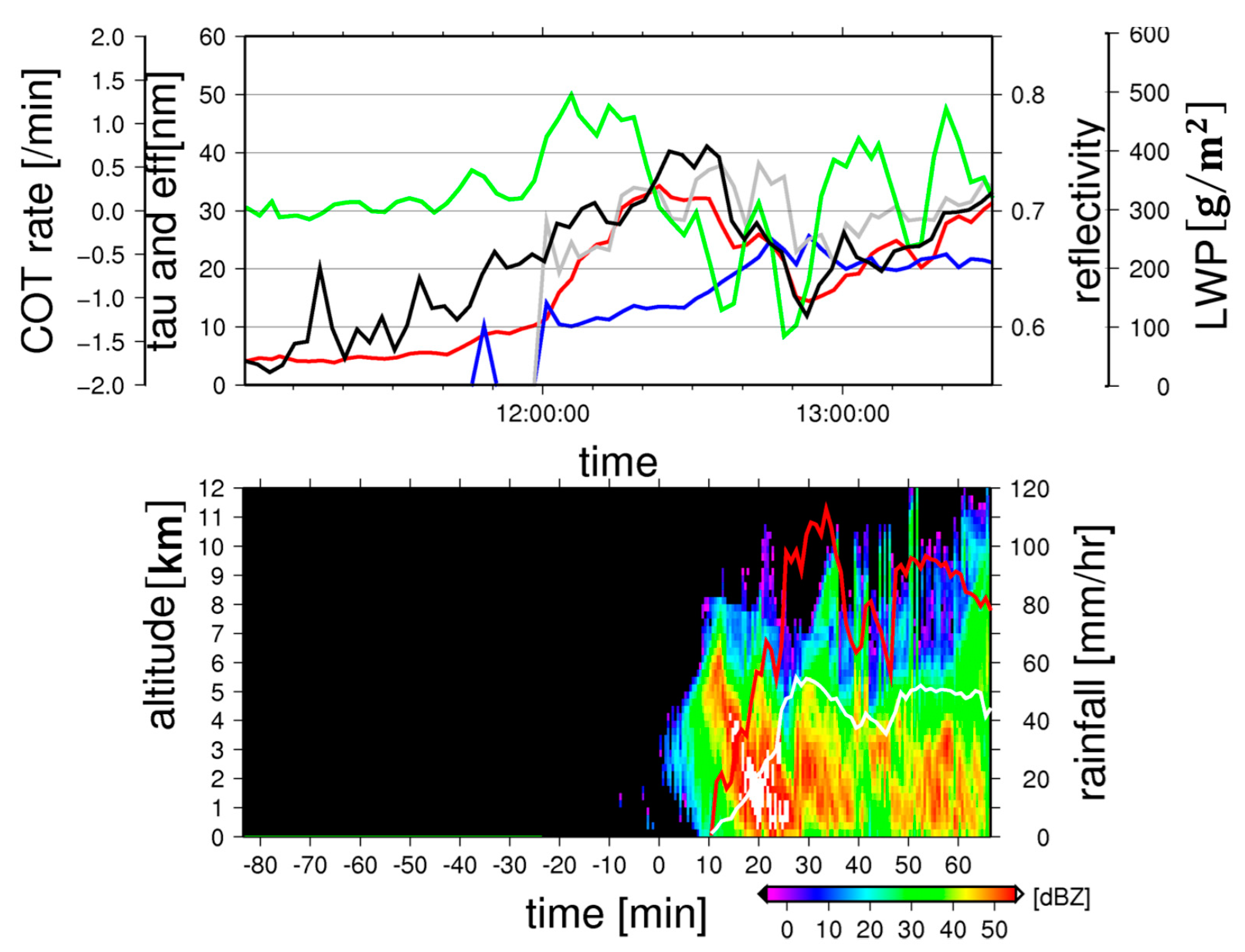
One of the features of third-generation GEOs is that they are multichannel, similar to MODIS. Such similarities mean that the optical characteristics of clouds (the optical thickness of clouds, and the effective radiative radius of cloud particles) estimated by optical sensors such as MODIS [56,57,58,59] can be applied to third-generation GEOs [60,61,62,63]. In addition, the synergistic observation of the same target by the multi-principle sensors called A-Train [64,65] can deepen the understanding of the cloud growth process [66,67,68] system by taking advantage of the characteristics of high-frequency observations. As a good example, the comprehensive observation of cloud and precipitation systems [69] in the Boso area, Chiba Prefecture, Japan, will be introduced. In the same area, X-band Phased Array Weather Radar (PAWR) was installed and operated to monitor the three-dimensional precipitation cell structure with a 30-s ultra-fine time resolution [70]. Figure 1 demonstrates the time evolution of the optical properties of a cloud system estimated by the cloud microphysical properties algorithm (CAPCOM) [71] (Figure 1, top), and the same time changes in the vertical profile of radar reflectivity captured by the PAWR (Figure 1, bottom), with the time of the first-echo detection by PAWR set to zero. Himawari-8 captured an apparent increase in cloud optical thickness (red line) starting 30 min before the first echo detection, and followed by a peak in visible reflectance (black line). The dramatic enhancement of the third-generation GEO provides a breakthrough in the better understanding cloud and precipitation processes by identifying the detail of cloud systems lifetime. In addition, attempts are made to refine the classification of cloud types proposed by the International Satellite Cloud Climatology Project (ISCCP) [72], by using the split windows method with multiband data and the brightness temperature difference parameter [73].
The enhanced functionality of third-generation GEOs has a substantial impact on weather forecasting with computer resource advancement and data assimilation [74,75,76]. One of the original purposes of GEOs was to calculate atmospheric moving vector winds, and they have contributed to the accuracy of weather forecasting by improving the atmospheric wind field. In addition, the Himawari-8 has a target area observation mode, especially for typhoons. It can make a high-frequency observation every 2.5 min [5]. Typhoons are a great source of material for machine learning because they cause significant damage by landing [77,78]. An excellent example of the combination of the development of machine learning and the enhancement of third-generation GEOs is the estimation of rain rate by the Himawari-8 using random-forest machine learning [79]. Hirose et al. [79] applied the methodology used initially for MSG to learn from ground-based radar data [80], and they succeeded in better reproducing precipitation with low storm height but heavy rain rate, which is often seen in wet areas [81], by utilizing the three-splitting bands in water vapor (WV) absorption bands around 7 µm. In addition, the improvement of precipitation estimation accuracy by nowcasting global precipitation products [82] using high-frequency observations may improve disaster prediction accuracy, mainly for flood event detection.
2.3.2. Dust Events and Aerosols
Precise monitoring of large-scale dust events in the temporal direction provides essential information for reducing the impact of dust on human activities [83]. Therefore, dust monitoring by satellite observations was conducted during the early satellite operation era [84]. Ackerman [85] described the utilization of tree bands in TIR (8.5, 11 (or 10), and 12 μm) for the detection of volcanic and soil-derived aerosols. The satellites have been used to generate RGB composite images (Dust RGB: ΔTbb 12.4–10.4 μm in red, ΔTbb 10.4–8.6 μm in green, and Tbb 10.4 μm in blue) by applying thermal infrared 3-band information. Because MSG and third-generation GEOs have achieved multiple bands in the thermal infrared region and increased observation frequencies, many studies on dust monitoring now use the brightness temperature difference in the thermal infrared region [86,87,88,89,90,91,92].
Aerosol optical parameters, such as aerosol optical thickness, can also be retrieved from optical sensors onboard satellites, although only during the daytime and only in areas without cloud cover [93,94,95,96,97,98,99]. The multi-band capability of third-generation GEOs has improved aerosol optical parameter estimation accuracy, and its use is expanding [100,101,102,103,104,105]. The aging of optical sensors’ sensitivity, which is essential for aerosol estimation, has been reported [106], and aerosol optical properties are steadily moving into the monitoring phase. Although aerosol optical properties and vertical structure of cloud-covered areas cannot be determined in principle, more detailed aerosol information in the spatio–temporal direction has been successfully derived by using the data assimilation technique as described in Section 2.3.1 [107,108,109]. It is noteworthy that the aerosol observation impact of third-generation GEOs can be derived to a greater extent through more advanced coordination with numerical forecast information.
2.3.3. Volcanic Plumes and Lightning Activity
It is essential to use satellite observations for disaster monitoring and immediate response in monitoring volcanic plumes, which are extremely difficult to predict in advance. Similar to the dust event monitoring described in Section 2.3.2, multi-band monitoring is effective by taking advantage of the aerosol ejection fraction (mostly SO2) emitted in an eruption, depending on the thermal infrared wavelength region [85,110]. It is helpful to summarize what approaches, including satellite observations, are effective for eruption monitoring, using the example of Eyjaföll volcano in Iceland, which erupted from 23 March to 14 April 2010 [111]. There are examples of utilizing the multi-band TIR channels in second-generation GEOs [112,113]. Monitoring examples by third-generation GEOs with increased observation frequency and number of bands, include the eruption of Aso Caldera in Japan on 8 October 2016, by Himawari-8 [114], and the eruption of Raung, Indonesia [115], focusing on the behavior of shorter wavelengths (1.6, 2.3, and 3.9 μm) [116].
From a natural disaster monitoring point of view, such as the effects of lightning strikes on electronic equipment and the causes of spontaneous ignition, lightning activity monitoring using satellites is also effective [117]. Because it can also be used as an indicator of atmospheric upwelling motion [118], a lightning imaging sensor (LIS) was installed on the Tropical Rainfall Measuring Mission (TRMM) [119,120]. The geostationary lightning mapper (GLM) was installed in the GOES-R series [121]. Preliminary observations of lightning captured by GLM have been obtained [122], and there are reports on lightning-related Fuego eruptions [123].
2.4. Target Phenomena for the Terrestrial Environment
2.4.1. Vegetation Activity and Forest Fires
The Landsat series was the first satellite to monitor terrestrial environments. The NOAA/AVHRR series of meteorological satellites separated the visible and near-infrared bands in the AVHRR/2 series. Thus, the normalized difference vegetation index (NDVI), which is a widely utilized vegetation index, can be applied. The NOAA/AVHRR could monitor vegetation dynamics globally in the early era of environmental remote sensing [124,125]. The generation of global datasets derived from the NOAA/AVHRR has begun to yield important insights into the response of vegetation to climate change [126,127], the application of satellite data for phenological timings [128], and fundamental studies of vegetation response to temperature and precipitation [129]. Our understanding of global environmental research has been enhanced by using highly accurate products produced by a well-organized MODIS science team for analysis [130]. However, the interpretation of tropical rainforests with frequent cloud cover is, for example, in contrast to the vegetation response of the Amazon rainforest to the 2005 drought [131,132], and increasing the frequency of cloud-free observations is considered to be the key to further understanding of vegetation response, especially in the tropics.
With an increase in the number of observation bands in MSG (Table 1) and an increase in the observation frequency (once every 15 min), the possibility of vegetation monitoring by GEO has greatly expanded. A series of investigations by Fensholt et al. [133,134,135] and others [136] have shown its usefulness. As evidence, the EUMETSAT provides vegetation indices such as leaf area index (LAI) from MSG [137], and expectations for vegetation monitoring by GEO with enhanced functions are high.
In the mid-latitudes, Miura et al. [138] monitored deciduous broadleaf trees in Japan by Himawari-8, and Wheeler and Dietze [139] by the GEOS-R series; this points to a dramatic increase in third-generation GEOs’ frequency of observations compared to LEOs (approximately 50 times more). Hashimoto et al. [140] conducted an analysis using GOES-16 on the Amazon rainforest. They demonstrated seasonal changes in NDVI in the Amazon rainforest, which could not be confirmed by conventional LEO, such as MODIS, due to the dramatic increase in the frequency of observations by GOES-R. Key to this result is the geometric correction [38,40,42] and atmospheric correction accuracies including in aerosols. For the latter, the standard atmospheric correction developed in MODIS (multiangle implementation of atmospheric correction (MAIAC) [141]) was adapted to GOES-R, and its usefulness was demonstrated by comparison with the local observation network “AERONET”. In terms of aerosol correction, there is room for further improvement in accuracy by utilizing the results obtained in atmospheric research [99,109], but the high computational cost is prohibitive in terms of providing data in quasi-real-time. To overcome this problem, further advances using AI, such as neural networks, are required. In addition, there is a more integrated relationship between GEOs and LEOs, and it is necessary for future applications to make a more sophisticated link between the high temporal frequency and low spatial resolution vegetation information obtained by GEOs, with research that looks at vegetation in a more detailed spatial direction (using LEO satellites such as Landsat, Satellite Pour l’Observation de la Terre (SPOT), and Sentinel [142]). For example, improving the spatial resolution of GEO by coupling the use of LEO optics is the one of potential utilization. Otherwise, based on LEO optics, phenological cycles interpolation with the assist of GEO data is another way.
One of the most effective applications that benefits from GEOs’ high temporal resolution and excellent latency to provide data, is forest fire monitoring [117]. There is a long history of forest fire monitoring by satellites [143,144], and the detection algorithms developed in MODIS [145,146] can be easily applied, as well as the algorithms developed in the second-generation GEOs [147]. It has been visualized in the JAXA Himawari Monitor [25] and the GOES-R standard product.
2.4.2. Land Surface Temperature (LST), Heat Islands, and Heatwaves
Estimating land surface temperature (LST) using the split windows method with multi-band NOAA/AVHRR thermal infrared has taken place since the early days when satellite observations began [148,149,150,151]. LST estimation using second-generation GEOs has also been conducted [152,153], and with third-generation GEOs, LST estimation methods that take advantage of the further multi-banding of TIR have been proposed [154,155,156,157]. As the frequency of observations increases dramatically, the removal of cloud pixels [158,159] becomes key to accurate LST estimation. Because GEOs can observe the diurnal cycle of LST at a higher frequency, it effectively analyzes the phenomena that cause daily changes, especially the factors that cause heat islands [160,161,162]. In addition, there is a possibility that third-generation GEOs can provide more detailed information in the time direction of the heatwave [163], which has been occurring increasingly in recent years. With LEOs, only a snapshot can be obtained, but with GEOs, for example, in principle it is possible to predict high LST duration times that can be harmful to the human body.
2.4.3. Landslides and Flooded Area Monitoring
The most acceptable resolution for third-generation GEOs is 500 m at the Nadir, which is equivalent to MODIS. By taking advantage of high-frequency observation characteristics, it is possible to monitor the general state of a large-scale disaster more quickly than any other satellite observation when the weather is clear. Miura and Nagai [164] demonstrated that landslides occurring after record-breaking heavy rainfall in Japan could be predicted by focusing on a rapid decrease in NDVI. The prediction of landslides based on changes in NDVI requires the original NDVI values to be high, and it is difficult to apply this method during the low NDVI periods of spring and fall in deciduous broadleaf forests, but it remains a highly effective approach.
As all third-generation GEOs are equipped with a 1.6 μm band, water-related monitoring, for example, flood area monitoring by calculating the normalized difference water index (NDWI) [165], is also possible in principle. Even without inter-band computation, it is possible to visualize a wide area of the flooded area using a natural color RGB composite by assigning a 1.6 μm band. In MSG, the resolution at 1.6 μm was 4 km, which was rough, but in third-generation GEOs, the resolution is 2 km, even in the 1.6 μm band, so more detailed information can be obtained.
3. Possible Further Collaboration between GEOs and LEOs—Case Study
Using the example of Typhoon Hagibis in 2019, which caused extensive flooding in Japan, we posed the question, “If we had been able to issue a high-resolution LEO observation request based on GEO information, how quickly would we have been able to acquire high-resolution observation images over the damaged area?” A simple simulation was conducted to answer this question. Please note that this is only a hypothetical check, and the assumptions presented here have not been explored in detail.
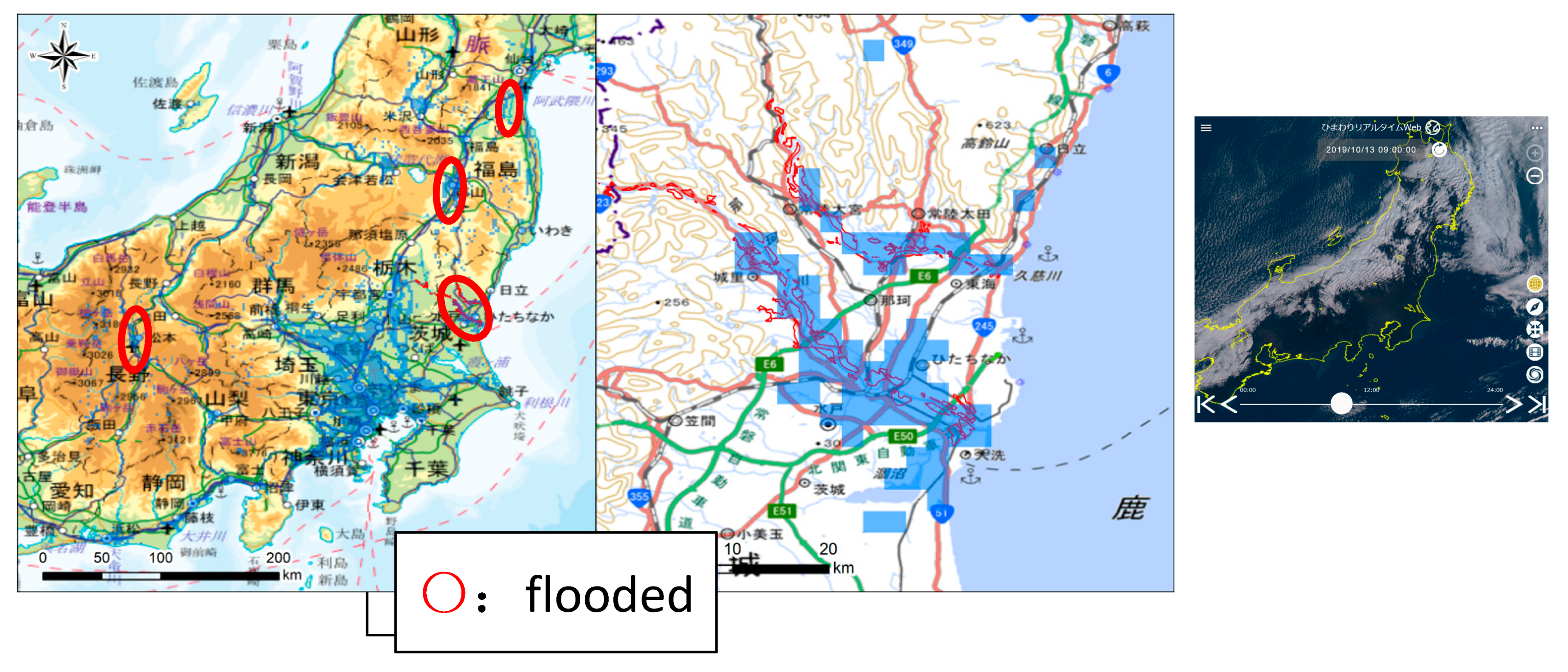
Typhoon Hagibis made landfall in Japan on 12 October 2019, reaching a minimum pressure of 915 hPa and causing extensive damage mainly in eastern Japan. This typhoon brought the heaviest daily precipitation recorded since 1982 at 613 comparable JMA observation sites, with a 24-h accumulated precipitation amount reaching 942.5 mm at Hakone. The death toll was 105, and according to the Ministry of Land, Infrastructure, Transport, and Tourism (MLIT), the area inundated by Hagibis reached approximately 25,000 ha in extent, exceeding the 18,500 ha by the extreme heavy rainfall event of July 2018 [166].
We first tried to extract the inundated area under a typhoon situation such as that of the case study, by hypothetically using Himawari-8 data. We used the Himawari-8 gridded FD data [41] provided by CEReS, Chiba University, Japan. Cloud removal used in the LST estimation algorithm [154] was performed, and the NDWI [165] was computed. To determine the threshold value of the flooded area, we used the map information of the flooded area visually identified by high-resolution optical sensors, and tentatively identified the pixels below −0.2 in the NDWI as the flooded area. Figure 2 shows the geographical map of the flooded area with an NDWI below −0.2 on the day after the Hagibis passage (09:00 Japan Standard Time (JST), 13 October 2019) captured in Himawari-8 true-color composite image from the Himawari real-time website at the same time. It can be seen that there were many misidentifications of inundated areas in the metropolitan urban areas, but the suburban areas appropriately reflected the inundated areas of rivers. The NDWI calculations were available from 06:00 JST on the same day, but due to the low solar elevation, the NDWI did not correctly represent the flooded area (figures are not shown), and although qualitatively, it showed an overestimation from 07:30 JST (figures are not shown).
Based on the observation information from Himawari-8, we hypothetically assumed the observation requirements for a commercial-based high-resolution optical satellite and a synthetic-aperture radar (SAR) satellite. On the one hand, for optical satellites, requests are accepted up to 03:00 JST on the same day, so in this case, it was difficult to determine the possible flooded area and issue an observation request on the same day (12 October). On the other hand, SAR requests can be accepted up to one hour before the command uplink, so it was possible to request observations by making a quick decision based on the NDWI flooded area information on the morning after typhoon Hagibis hit. This showed that disaster monitoring could be organically linked to LEO observations by using GEO observation information more appropriately than has been done to date.
4. Closing Remarks and Future Perspectives
A review was conducted focusing on third-generation GEOs, with visualization (RGB full-color composite, visualization via the web interface), baseline dataset, and phenomena to be covered limited to the atmospheric and terrestrial environments. For both atmospheric and terrestrial environments, enhanced capabilities of third-generation GEO were found to provide critical information for disaster management and risk mitigation. In particular, it is essential to reiterate that GEO data make a better contribution to bridging the gap between observation data and virtual data such as numerical forecasts, through the latest technologies such as data assimilation and Artificial Intelligence (AI). The improvement of near-future forecast with the assist of GEO data implicitly contributes to disaster risk mitigations. Numerical simulations of hydrological processes using global precipitation datasets as inputs [167,168], which also utilize GEO data such as GSMaP, are also highly effective for risk mitigation of flood damage, and further integration of satellite observation and numerical prediction, not limited to GEO, is an excellent way to mitigate damage caused by disasters.
According to the Vision for the World Meteorological Organization (WMO) Integrated Global Observing System in 2040 [169], there are four types of sensors that should be onboard geostationary meteorological satellites by the year 2040: (1) high-frequency, multi-wavelength imagers or radiometers; (2) hyperspectral infrared sounders; (3) lightning imagers; and (4) ultraviolet, visible, and near-infrared sounders. By achieving this, hyperspectral infrared sounder observations will, for example, be able to provide more frequent and accurate information on the vertical profiles of temperature and water vapor in clear-sky pixels. Using this information, the accuracy of the atmospheric correction of optical sensors can be drastically improved.
The enhancement of functions by third-generation GEOs has resulted in a dramatic expansion in data volume, and some GEOs have started to provide data through cloud services, but even in the context of citizen science, the general use of third-generation GEOs is still low compared to the high level of interest shown in it. Putting aside the issue of who is responsible for associated costs, it is essential to establish a system where the data can be used in a broader range, considering the amount of publicity it has achieved and the need for its immediate use.
Funding
The author is partly supported by Grants-in-Aid for Scientific Research (grant number 20K04080) from the Japan Society for the Promotion of Science (JSPS) and Precipitation Measurement Mission/RA (grant number JX-PSPC-519794) from the Japan Aerospace Exploration Agency (JAXA), and collaborative work between PASCO CORPORATION (PASCO) and Chiba University for “Research on Extraction and Visualization of Floodable Area Using Himawari Satellite and Operation of Earth-Orbiting Satellite”.
Institutional Review Board Statement
Not applicable.
Informed Consent Statement
Informed consent was obtained from all subjects involved in the study.
Data Availability Statement
The data analyzed in Figure 1 and Figure 2 are partly available. Himawari-8 base gridded data can be accessed via the Internet [41]. The Himawari-8 analyzed dataset, the so-called AMATERASS, can be accessed via the NPO solar radiation consortium (http://www.amaterass.org/, accessed on 19 March 2021). XRAIN data can also be accessed via the Data Integration and Analysis System Program (DIAS) (https://diasjp.net/en/, accessed on 19 March 2021). PAWR data were obtained from Japan Radio Co. (JRC) Ltd., with data policies decided by the JRC. Validation data for determination of the NDWI threshold were obtained from PASCO with data policies decided by PASCO.
Acknowledgments
Hideaki Takenaka, CEReS Chiba University, provided the Himawari-8 oriented cloud optical properties dataset through the NPO solar radiation consortium. PAWR data were provided by Kazuomi Morotomi and Shigeharu Shimamura of Japan Radio Co. Ltd., Japan. The XRAIN data were obtained from DIAS. Hitoshi Nozawa, a student at Chiba University, analyzed the dataset shown in Figure 1. Takashi Shibayama and Hiroto Kikuchi, Yoshiki Hamaguchi of PASCO, and Yuhei Yamamoto and Ryotaro Suzuki of CEReS, Chiba University conducted the data analysis in Section 3. The author appreciates their contributions.
Conflicts of Interest
The author declares no conflict of interest.
References
- Kidder, S.Q.; Vonder Haar, T.H. Satellite Meteorology, an Introduction; Academic Press, Inc.: San Diego, CA, USA, 1995; p. 466. [Google Scholar]
- Suomi, V.E.; Parent, R. A color view of Planet Earth. Bull. Am. Meteorol. Soc. 1968, 49, 74–75. [Google Scholar] [CrossRef] [Green Version]
- Schmit, T.J.; Griffith, P.; Gunshor, M.M.; Daniels, J.M.; Goodman, S.J.; Lebair, W.J. A closer look at the ABI on the GOES-R series. Bull. Am. Meteorol. Soc. 2017, 98, 681–698. [Google Scholar] [CrossRef]
- Kodaira, N.; Murayama, N.; Yamashita, H.; Kohno, T. On the Geostationary Meteorological Satellite. GMS (Himawari). Tenki 1978, 25, 245–268. (In Japanese) [Google Scholar]
- Bessho, K.; Date, K.; Hayashi, M.; Ikeda, A.; Imai, T.; Inoue, H.; Kumagai, Y.; Miyakawa, T.; Murata, H.; Ohno, T.; et al. An introduction to Himawari-8/9 Japan’s new-generation geostationary meteorological satellites. J. Meteorol. Soc. Jpn. 2016, 94, 151–183. [Google Scholar] [CrossRef] [Green Version]
- Menzel, W.P.; Purdom, J.F.W. Introducing GOES-I: The first of a new generation of Geostationary Operational Environmental Satellites. Bull. Am. Meteorol. Soc. 1994, 75, 757–782. [Google Scholar] [CrossRef] [Green Version]
- Puschell, J.J.; Lowe, H.A.; Jeter, J.W.; Kus, S.M.; Hurt, W.T.; Gilman, D.; Rogers, D.L.; Hoelter, R.L.; Ravella, R. Japanese Advanced Meteorological Imager: A next-generation GEO imager for MTSAT-1R. In Earth Observing Systems VII, Proceedings of the International Symposium on Optical Science and Technology, Seattle, WA, USA, 7–11 July 2002; SPIE: Bellingham, WA, USA, 2002; Volume 4814. [Google Scholar] [CrossRef]
- Inoue, T. A cloud type classification with NOAA 7 split-window measurements. J. Geophys. Res. 1987, 92, 3991–4000. [Google Scholar] [CrossRef]
- Ohsawa, T.; Ueda, H.; Hayashi, T.; Watanabe, A.; Matsumoto, J. Diurnal variations of convective activity and rainfall in Tropical Asia. J. Meteorol. Soc. Jpn. 2001, 79, 333–352. [Google Scholar] [CrossRef] [Green Version]
- Hirose, H.; Yamamoto, M.K.; Shige, S.; Higuchi, A.; Mega, T.; Ushio, T.; Hamada, A. A rain potential map with high temporal and spatial resolutions retrieved from five geostationary meteorological satellites. SOLA 2016, 12, 297–301. [Google Scholar] [CrossRef] [Green Version]
- Schmetz, J.; Pili, P.; Tjemkes, S.; Just, D.; Kerkmann, J.; Rota, S.; Ratier, A. An introduction to Meteosat Second Generation (MSG). Bull. Am. Meteorol. Soc. 2002, 83, 977–992. [Google Scholar] [CrossRef]
- Yang, J.; Zhang, Z.; Wei, C.; Lu, F.; Guo, Q. Introducing the new generation of Chinese geostationary weather satellites, Fengyun-4. Bull. Am. Meteorol. Soc. 2017, 98, 1637–1658. [Google Scholar] [CrossRef]
- Aminou, D.M.; Lamarre, D.; Stark, H.; Braembussche, P.V.D.; Blythe, P.; Fowler, G.; Gigli, S.; Stuhlmann, R.; Rota, S. Meteosat Third Generation (MTG) status of space segment definition. In Sensors, Systems, and Next-Generation Satellites XIII, Proceedings of the SPIE Remote Sensing, Berlin, Germany, 31 August–3 September 2009; SPIE: Bellingham, WA, USA, 2009; Volume 7474, p. 747406. [Google Scholar] [CrossRef]
- Miller, S.D.; Schmit, T.L.; Seaman, C.J.; Lindsey, D.T.; Gunshor, M.M.; Kohrs, R.A.; Sumida, Y.; Hillger, D. A sight for sore eyes: The return of true color to geostationary satellites. Bull. Am. Meteorol. Soc. 2016, 97, 1803–1816. [Google Scholar] [CrossRef]
- Bah, M.K.; Gunshor, M.M.; Schmit, T.J. Generation of GOES-16 true color imagery without a green band. Earth Space Sci. 2018, 5, 549–558. [Google Scholar] [CrossRef]
- Murata, H.; Saitoh, K.; Sumida, Y. True color imagery rendering for Himawari-8 with a color reproduction approach based on the CIE XYZ color system. J. Meteorol. Soc. Jpn. 2018, 96B, 211–238. [Google Scholar] [CrossRef] [Green Version]
- Broomhall, M.A.; Majewski, L.J.; Villani, V.O.; Grant, I.F.; Miller, S.D. Correcting Himawari-8 Advanced Himawari Imager data for the production of vivid true-color imagery. J. Atmos. Ocean. Technol. 2019, 36, 427–442. [Google Scholar] [CrossRef]
- Miller, S.D.; Lindsey, D.T.; Seaman, C.J.; Solbrig, J.E. GeoColor: A blending technique for satellite imagery. J. Atmos. Ocean. Technol. 2020, 37, 429–448. [Google Scholar] [CrossRef]
- EUMETSAT. Complication of RGB Recipies, How to Create the Standard RGB Images from METEOSAT/SEVIRI and MetOp/AVHRR and VIIRS Data? Available online: http://www.eumetrain.org/RGBguide/recipes/RGB_recipes.pdf (accessed on 4 March 2021).
- JMA. RGB Training Library. Available online: http://www.jma.go.jp/jma/jma-eng/satellite/RGB_TL.html (accessed on 4 March 2021).
- COMET MetEd. Multispectral Satellite Applications: RGB Products Explained. Available online: https://www.meted.ucar.edu/training_module.php?id=568&tab=01#.YEDIhuZUtR5 (accessed on 4 March 2021).
- Murata, K.T.; Pavarangkoon, P.; Higuchi, A.; Toyoshima, K.; Yamamoto, K.; Muranaga, K.; Nagaya, Y.; Izumikawa, Y.; Kimura, E.; Mizuhara, T. A web-based real-time and full-resolution data visualization for Himawari-8 satellite sensed images. Earth Sci. Inform. 2018, 11, 217–237. [Google Scholar] [CrossRef] [Green Version]
- Pavarangkoon, P.; Murata, K.T.; Yamamoto, K.; Muranaga, K.; Higuchi, A.; Mizuhara, T.; Kagebayashi, Y.; Charnsripinyo, C.; Nupairoj, N.; Ikeda, T.; et al. Development of international mirroring system for real-time web of meteorological satellite data. Earth Sci. Inform. 2020, 13, 1461–1476. [Google Scholar] [CrossRef]
- NICT Science Cloud Team. Himawari Real-Time Web. Available online: https://himawari8.nict.go.jp/ (accessed on 5 March 2021).
- JAXA Himawari Monitor. Available online: https://www.eorc.jaxa.jp/ptree/ (accessed on 5 March 2021).
- JMA Himawari Monitor. Available online: https://www.jma.go.jp/bosai/map.html#contents=himawari&lang=en (accessed on 5 March 2021).
- NOAA. GOES Image Viewer. Available online: https://www.star.nesdis.noaa.gov/GOES/index.php (accessed on 5 March 2021).
- JMA. Dissemination and Distribution. Available online: https://www.jma.go.jp/jma/jma-eng/satellite/dissemination.html (accessed on 11 March 2021).
- NOAA. Data Access for GOES-R Series Satellites. Available online: https://www.ncdc.noaa.gov/data-access/satellite-data/goes-r-series-satellites (accessed on 11 March 2021).
- EUMETSAT. How to Access Our Data. Available online: https://www.eumetsat.int/access-our-data (accessed on 11 March 2021).
- Japan Meteorological Business Support Center (JMBSC) Service. Available online: http://www.jmbsc.or.jp/en/index-e.html (accessed on 11 March 2021).
- NOAA. GOES-R Series Satellite Data in the NOAA Big Data Project. Available online: https://www.ncdc.noaa.gov/data-access/satellite-data/satellite-data-noaa-big-data-project (accessed on 11 March 2021).
- AWS Public Sector Blog Team. Accessing NOAA’s GOES-R Series Satellite Weather Imagery Data on AWS. 2017. Available online: https://aws.amazon.com/jp/blogs/publicsector/accessing-noaas-goes-r-series-satellite-weather-imagery-data-on-aws/ (accessed on 11 March 2021).
- JMA Meteorological Satellite Center. Sample Data and Sample Source Code. Available online: https://www.data.jma.go.jp/mscweb/en/himawari89/space_segment/spsg_sample.html (accessed on 11 March 2021).
- Space Science and Engineering Center, University of Wisconsin-Madison. Community Satellite Processing Package for Geostationary Data (CSPP Geo). Available online: http://cimss.ssec.wisc.edu/csppgeo/ (accessed on 11 March 2021).
- Okuyama, A.; Andou, A.; Date, K.; Hoasaka, K.; Mori, N.; Murata, H.; Tabata, T.; Takahashi, M.; Yoshino, R.; Bessho, K. Preliminary validation of Himawari-8/AHI navigation and calibration. In Earth Observing Systems XX, Proceedings of the SPIE Optical Engineering + Applications, San Diego, CA, USA, 9–13 August 2015; SPIE: Bellingham, WA, USA, 2015; Volume 9607, p. 96072E. [Google Scholar] [CrossRef]
- Tan, B.; Dellomo, J.; Wolfe, R.; Reth, A. GOES-16 ABI navigation assessment. In Earth Observing Systems XXIII, Proceedings of the SPIE Optical Engineering + Applications, San Diego, CA, USA, 19–23 August 2018; SPIE: Bellingham, WA, USA, 2018; Volume 10764, p. 107640G. [Google Scholar] [CrossRef]
- Takenaka, H.; Sakashita, T.; Higuchi, A.; Nakajima, T. Geolocation correction for geostationary satellite observations by a phase-only correlation method using a visible channel. Remote Sens. 2020, 12, 2472. [Google Scholar] [CrossRef]
- Foroosh, H.; Zerubia, J.; Berthod, M. Extension of phase correlation to subpixel registration. IEEE Trans. Image Process. 2002, 11, 188–200. [Google Scholar] [CrossRef] [Green Version]
- Wang, W.; Li, S.; Hashimoto, H.; Takenaka, H.; Higuchi, A.; Kalluri, S.; Nemani, R. An introduction to the Geostationary–NASA Earth Exchange (GeoNEX) products: 1. Top-of-Atmosphere reflectance and brightness temperature. Remote Sens. 2020, 12, 1267. [Google Scholar] [CrossRef] [Green Version]
- Center for Environmental Remote Sensing, Chiba University. Release Note of “Himawari 8” Gridded Data for Full-Disk (FD) Observation Mode. Available online: http://www.cr.chiba-u.jp/databases/GEO/H8_9/FD/ (accessed on 11 March 2021).
- Yamamoto, Y.; Ichii, K.; Higuchi, A.; Takenaka, H. Geolocation accuracy assessment of Himawari-8/AHI imagery for application to terrestrial monitoring. Remote Sens. 2020, 12, 1372. [Google Scholar] [CrossRef]
- Liu, Z.; Ostrenga, D.; Teng, W.; Kempler, S. Tropical Rainfall Measuring Mission (TRMM) precipitation data and services for research and applications. Bull. Am. Meteorol. Soc. 2012, 93, 1317–1325. [Google Scholar] [CrossRef] [Green Version]
- Liu, Z.; Shie, C.-L.; Li, A.; Meyer, D. NASA global satellite and model data products and services for tropical meteorology and climatology. Remote Sens. 2020, 12, 2821. [Google Scholar] [CrossRef]
- Knapp, K.R.; Ansari, S.; Bain, C.L.; Bourassa, M.A.; Dickinson, M.J.; Funk, C.; Helms, C.N.; Hennon, C.C.; Holmes, C.D.; Huffman, G.J.; et al. Globally gridded satellite (GridSat) observations for climate studies. Bull. Am. Meteorol. Soc. 2011, 92, 893–907. [Google Scholar] [CrossRef]
- Knapp, K.R.; Wilkins, S. Gridded Satellite (GridSat) GOES and CONUS data. Earth Syst. Sci. Data 2018, 10, 1417–1425. [Google Scholar] [CrossRef] [Green Version]
- Nitta, T.; Sekine, S. Diurnal variation of convective activity over the Tropical Western Pacific. J. Meteorol. Soc. Jpn. 1994, 72, 627–641. [Google Scholar] [CrossRef] [Green Version]
- Fujinami, H.; Yasunari, T. The seasonal and intraseasonal variability of diurnal cloud activity over the Tibetan Plateau. J. Meteorol. Soc. Jpn. 2001, 79, 1207–1227. [Google Scholar] [CrossRef] [Green Version]
- Kurosaki, Y.; Kimura, F. Relationship between topography and daytime cloud activity around Tibetan Plateau. J. Meteorol. Soc. Jpn. 2002, 80, 1339–1355. [Google Scholar] [CrossRef] [Green Version]
- Kondo, Y.; Higuchi, A.; Nakamura, K. Small-scale cloud activity over the Maritime Continent and the Western Pacific as revealed by satellite data. Mon. Weather Rev. 2006, 134, 1581–1599. [Google Scholar] [CrossRef]
- Inoue, T.; Vila, D.; Rajendran, K.; Hamada, A.; Wu, X.; Machado, L.A.T. Life cycle of deep convective systems over the Eastern Tropical Pacific observed by TRMM and GOES-W. J. Meteorol. Soc. Jpn. 2009, 87A, 381–391. [Google Scholar] [CrossRef] [Green Version]
- Imaoka, K.; Nakamura, K. Statistical analysis of the life cycle of isolated tropical cold cloud systems using MTSAT-1R and TRMM data. Mon. Weather Rev. 2012, 140, 3552–3572. [Google Scholar] [CrossRef]
- Senf, F.; Deneke, H. Satellite-based characterization of convective growth and glaciation and its relationship to precipitation formation over central Europe. J. Appl. Meteorol. Climatol. 2017, 56, 1827–1845. [Google Scholar] [CrossRef]
- Hamada, A.; Takayabu, Y.N. Convective cloud top vertical velocity estimated from geostationary satellite rapid-scan measurements. Geophys. Res. Lett. 2016, 43, 5435–5441. [Google Scholar] [CrossRef] [Green Version]
- Gallucci, D.; De Natale, M.P.; Cimini, D.; Di Paola, F.; Gentile, S.; Geraldi, E.; Larosa, S.; Nilo, S.T.; Ricciardelli, E.; Viggiano, M.; et al. Convective initiation proxies for nowcasting precipitation severity using the MSG-SEVIRI rapid scan. Remote Sens. 2020, 12, 2562. [Google Scholar] [CrossRef]
- Nakajima, T.Y.; Nakajima, T. Wide-area determination of cloud microphysical properties from NOAA AVHRR measurements for FIRE and ASTEX regions. J. Atmos. Sci. 1995, 52, 4043–4059. [Google Scholar] [CrossRef] [Green Version]
- Nakajima, T.Y.; Nakajima, T.; Nakajima, M.; Fukushima, H.; Kuji, M.; Uchiyama, A.; Kishino, M. Optimization of the Advanced Earth Observing Satellite II Global Imager channels by use of radiative transfer calculations. Appl. Opt. 1998, 37, 3149–3163. [Google Scholar] [CrossRef] [PubMed]
- Nakajima, T.Y.; Suzuki, K.; Stephens, G.L. Droplet growth in warm water clouds observed by the A-Train. Part I: Sensitivity analysis of the MODIS-derived cloud droplet size. J. Atmos. Sci. 2010, 67, 1884–1896. [Google Scholar] [CrossRef]
- Iwabuchi, H.; Saito, M.; Tokoro, Y.; Putri, N.S.; Sekiguchi, M. Retrieval of radiative and microphysical properties of cloud from multispectral infrared measurements. Prog. Earth Planet. Sci. 2016, 3, 32. [Google Scholar] [CrossRef] [Green Version]
- Iwabuchi, H.; Putri, N.S.; Saito, M.; Tokoro, Y.; Sekiguchi, M.; Yang, P.; Baum, B.A. Cloud property retrieval from multiband infrared measurements by Himawari-8. J. Meteorol. Soc. Jpn. 2018, 96B, 27–42. [Google Scholar] [CrossRef] [Green Version]
- Putri, N.S.; Iwabuchi, H.; Hayasaka, T. Evolution of mesoscale convective system properties as derived from Himawari-8 high resolution data analyses. J. Meteorol. Soc. Jpn. 2018, 96B, 239–250. [Google Scholar] [CrossRef] [Green Version]
- Khatri, P.; Hayasaka, T.; Iwabuchi, H.; Takamura, T.; Irie, H.; Nakajima, T.Y. Validation of MODIS and AHI observed water cloud properties using surface radiation data. J. Meteorol. Soc. Jpn. 2018, 96B, 151–172. [Google Scholar] [CrossRef] [Green Version]
- Letu, H.; Yang, K.; Nakajima, T.Y.; Ishimoto, H.; Nagao, T.M.; Riedi, J.; Baran, A.J.; Ma, R.; Wang, T.; Shang, H.; et al. High-resolution retrieval of cloud microphysical properties and surface solar radiation using Himawari-8/AHI next-generation geostationary satellite. Remote Sens. Environ. 2020, 239, 111583. [Google Scholar] [CrossRef]
- Stephens, G.L.; Vane, D.G.; Boain, R.J.; Mace, G.G.; Sassen, K.; Wang, Z.; Illingworth, A.J.; O’connor, E.J.; Rossow, W.B.; Durden, S.L.; et al. The CloudSat Mission and the A-TRAIN: A new dimension of space-based observations of clouds and precipitation. Bull. Am. Meteorol. Soc. 2002, 83, 1771–1790. [Google Scholar] [CrossRef] [Green Version]
- Stephens, G.; Winker, D.; Pelon, J.; Trepte, C.; Vane, D.; Yuhas, C.; L’Ecuyer, T.; Lebsock, M. CloudSat and CALIPSO within the A-Train: Ten years of actively observing the Earth system. Bull. Am. Meteorol. Soc. 2018, 99, 569–581. [Google Scholar] [CrossRef] [Green Version]
- Nakajima, T.Y.; Suzuki, K.; Stephens, G.L. Droplet growth in warm water clouds observed by the A-Train. Part II: A Multi-sensor view. J. Atmos. Sci. 2010, 67, 1897–1907. [Google Scholar] [CrossRef]
- Suzuki, K.; Nakajima, T.Y.; Stephens, G.L. Particle growth and drop collection efficiency of warm clouds as inferred from joint CloudSat and MODIS observations. J. Atmos. Sci. 2010, 67, 3019–3032. [Google Scholar] [CrossRef]
- Nagao, T.M.; Suzuki, K. Identifying particle growth processes in marine low clouds using spatial variances of imager-derived cloud parameters. Geophys. Res. Lett. 2020, 47, e2020GL087121. [Google Scholar] [CrossRef] [Green Version]
- Kobayashi, F.; Takano, T.; Takamura, T. Isolated cumulonimbus initiation observed by 95-GHz FM-CW radar, X-band radar, and photogrammetry in the Kanto Region, Japan. SOLA 2011, 7, 125–128. [Google Scholar] [CrossRef] [Green Version]
- Morotomi, K.; Shimamura, S.; Kobayashi, F.; Takamura, T.; Takano, T.; Higuchi, A.; Iwashita, H. Evolution of a tornado and debris ball associated with Super Typhoon Hagibis 2019 observed by X-band Phased Array Weather Radar in Japan. Geophys. Res. Lett. 2020, 47, e2020GL091061. [Google Scholar] [CrossRef]
- Nakajima, T.Y.; Ishida, H.; Nagao, T.M.; Hori, M.; Letu, H.; Higuchi, R.; Tamaru, N.; Imoto, N.; Yamazaki, A. Theoretical basis of the algorithms and early phase results of the GCOM-C (Shikisai) SGLI cloud products. Prog. Earth Planet. Sci. 2019, 6, 52. [Google Scholar] [CrossRef]
- Schiffer, R.A.; Rossow, W.B. The International Satellite Cloud Climatology Project (ISCCP): The first project of the World Climate Research Programme. Bull. Am. Meteorol. Soc. 1983, 64, 779–784. [Google Scholar] [CrossRef] [Green Version]
- Purbantoro, B.; Aminuddin, J.; Manago, N.; Toyoshima, K.; Lagrosas, N.; Sumantyo, J.; Kuze, H. Comparison of cloud type classification with split window algorithm based on different infrared band combinations of Himawari-8 satellite. Adv. Remote Sens. 2018, 7, 218–234. [Google Scholar] [CrossRef] [Green Version]
- Honda, T.; Miyoshi, T.; Lien, G.; Nishizawa, S.; Yoshida, R.; Adachi, S.A.; Terasaki, K.; Okamoto, K.; Tomita, H.; Bessho, K. Assimilating all-sky Himawari-8 satellite infrared radiances: A case of Typhoon Soudelor (2015). Mon. Weather Rev. 2018, 146, 213–229. [Google Scholar] [CrossRef]
- Zhang, Y.; Zhang, F.; Stensrud, D.J. Assimilating all-sky infrared radiances from GOES-16 ABI using an ensemble Kalman filter for convection-allowing severe thunderstorms prediction. Mon. Weather Rev. 2018, 146, 3363–3381. [Google Scholar] [CrossRef]
- Okamoto, K.; Sawada, Y.; Kunii, M. Comparison of assimilating all-sky and clear-sky infrared radiances from Himawari-8 in a mesoscale system. Q. J. Roy. Meteorol. Soc. 2019, 145, 745–766. [Google Scholar] [CrossRef]
- Chen, B.; Chen, B.; Lin, H.; Elsberry, R.L. Estimating tropical cyclone intensity by satellite imagery utilizing convolutional neural networks. Weather Forecast. 2019, 34, 447–465. [Google Scholar] [CrossRef]
- Chen, R.; Zhang, W.; Wang, X. Machine learning in tropical cyclone forecast modeling: A review. Atmosphere 2020, 11, 676. [Google Scholar] [CrossRef]
- Hirose, H.; Shige, S.; Yamamoto, M.K.; Higuchi, A. High temporal rainfall estimations from Himawari-8 multiband observations using the random-forest machine-learning method. J. Meteorol. Soc. Jpn. 2019, 97, 689–710. [Google Scholar] [CrossRef] [Green Version]
- Kühnlein, M.; Appelhans, T.; Thies, B.; Nauß, T. Precipitation estimates from MSG SEVIRI daytime, nighttime, and twilight data with random forests. J Appl. Meteorol. Climatol. 2014, 53, 2457–2480. [Google Scholar] [CrossRef] [Green Version]
- Hamada, A.; Takayabu, Y.; Liu, C.; Zipser, E.J. Weak linkage between the heaviest rainfall and tallest storms. Nat. Commun. 2015, 6, 6213. [Google Scholar] [CrossRef]
- Kubota, T.; Aonashi, K.; Ushio, T.; Shige, S.; Takayabu, Y.N.; Kachi, M.; Arai, Y.; Tashima, T.; Masaki, T.; Kawamoto, N.; et al. Global Satellite Mapping of Precipitation (GSMaP) products in the GPM era. In Satellite Precipitation Measurement; Springer: Berlin/Heidelberg, Germany, 2020; pp. 355–373. [Google Scholar]
- Kurosaki, Y.; Mikami, M. Recent frequent dust events and their relation to surface wind in East Asia. Geophys. Res. Lett. 2003, 30, 1736. [Google Scholar] [CrossRef]
- Legrand, M.; Bertrand, J.J.; Desbois, M.; Menenger, L.; Fouquart, Y. The potential of infrared satellite data for the retrieval of Saharan-dust optical depth over Africa. J. Appl. Meteorol. Climatol. 1989, 28, 309–319. [Google Scholar] [CrossRef] [Green Version]
- Ackerman, S.A. Remote sensing aerosols using satellite infrared observations. J. Geophys. Res. 1997, 102, 17069–17079. [Google Scholar] [CrossRef]
- Marchese, F.; Sannazzaro, F.; Falconieri, A.; Filizzola, C.; Pergola, N.; Tramutoli, V. An enhanced satellite-based algorithm for detecting and tracking dust outbreaks by means of SEVIRI data. Remote Sens. 2017, 9, 537. [Google Scholar] [CrossRef] [Green Version]
- Miller, S.D.; Bankert, R.L.; Solbrig, J.E.; Forsythe, J.M.; Noh, Y.-J. A dynamic enhancement with background reduction algorithm: Overview and application to satellite-based dust storm detection. J. Geophys. Res. Atmos. 2017, 122, 12938–12959. [Google Scholar] [CrossRef]
- Minamoto, Y.; Nakamura, K.; Wang, M.; Kawai, K.; Ohara, K.; Noda, J.; Davaanyam, E.; Sugimoto, N.; Kai, K. Large-scale dust event in East Asia in May 2017: Dust emission and transport from multiple source regions. SOLA 2018, 14, 33–38. [Google Scholar] [CrossRef] [Green Version]
- She, L.; Xue, Y.; Yang, X.; Guang, J.; Li, Y.; Che, Y.; Fan, C.; Xie, Y. Dust detection and intensity estimation using Himawari-8/AHI observation. Remote Sens. 2018, 10, 490. [Google Scholar] [CrossRef] [Green Version]
- Berndt, E.; Elmer, N.; Schultz, L.; Molthan, A. A methodology to determine recipe adjustments for multispectral composites derived from next-generation advanced satellite imagers. J. Atmos. Ocean. Technol. 2018, 35, 643–664. [Google Scholar] [CrossRef]
- Jee, J.B.; Lee, K.T.; Lee, K.H.; Zo, I.S. Development of GK-2A AMI aerosol detection algorithm in the East-Asia region using Himawari-8 AHI data. Asia-Pac. J. Atmos. Sci. 2020, 56, 207–223. [Google Scholar] [CrossRef]
- Sowden, M.; Blake, D. Which dual-band infrared indices are optimum for identifying aerosol compositional change using Himawari-8 data? Atmos. Environ. 2020, 241, 117620. [Google Scholar] [CrossRef]
- Nakajima, T.; Tanaka, M. Matrix formulations for the transfer of solar radiation in a plane-parallel scattering atmosphere. J. Quant. Spectrosc. Radiat. Trans. 1986, 35, 13–21. [Google Scholar] [CrossRef]
- Kaufman, Y.J.; Tanré, D.; Gordon, H.R.; Nakajima, T.; Lenoble, J.; Frouin, R.; Grassl, H.; Herman, B.M.; King, M.D.; Teillet, P.M. Passive remote sensing of tropospheric aerosol and atmospheric correction for the aerosol effect. J. Geophys. Res. 1997, 102, 16815–16830. [Google Scholar] [CrossRef] [Green Version]
- Tanré, D.; Kaufman, Y.J.; Herman, M.; Mattoo, S. Remote sensing of aerosol properties over oceans using the MODIS/EOS spectral radiances. J. Geophys. Res. 1997, 102, 16971–16988. [Google Scholar] [CrossRef]
- Higurashi, A.; Nakajima, T. Development of a two-channel aerosol retrieval algorithm on a global scale using NOAA AVHRR. J. Atmos. Sci. 1999, 56, 924–941. [Google Scholar] [CrossRef]
- Kaufman, Y.J.; Gobron, N.; Pinty, B.; Widlowski, J.L.; Verstraete, M.M. Relationship between surface reflectance in the visible and mid-IR used in MODIS aerosol algorithm-Theory. Geophys. Res. Lett. 2002, 29, 2116. [Google Scholar] [CrossRef] [Green Version]
- Remer, L.A.; Kaufman, Y.J.; Tanrré, D.; Mattoo, S.; Chu, D.A.; Martins, J.V.; Li, R.-R.; Ichoku, C.; Levy, R.C.; Kleidman, R.G.; et al. The MODIS aerosol algorithm, products, and validation. J. Atmos. Sci. 2005, 62, 947–973. [Google Scholar] [CrossRef] [Green Version]
- Hashimoto, M.; Nakajima, T. Development of a remote sensing algorithm to retrieve atmospheric aerosol properties using multiwavelength and multipixel information. J. Geophys. Res. Atmos. 2017, 122, 6347–6378. [Google Scholar] [CrossRef] [Green Version]
- Yoshida, M.; Kikuchi, M.; Nagao, T.M.; Murakami, H.; Nomaki, T.; Higurashi, A. Common retrieval of aerosol properties for imaging satellite sensors. J. Meteorol. Soc. Jpn. 2018, 96B, 193–209. [Google Scholar] [CrossRef] [Green Version]
- Kikuchi, M.; Murakami, H.; Suzuki, K.; Nagao, T.M.; Higurashi, A. Improved hourly estimates of aerosol optical thickness using spatiotemporal variability derived from Himawari-8 geostationary satellite. IEEE Trans. Geosci. Remote Sens. 2018, 56, 3442–3455. [Google Scholar] [CrossRef]
- Zhang, Z.; Fan, M.; Wu, W.; Wang, Z.; Tao, M.; Wei, J.; Wang, Q. A simplified aerosol retrieval algorithm for Himawari-8 Advanced Himawari Imager over Beijing. Atmos. Environ. 2019, 199, 127–135. [Google Scholar] [CrossRef]
- Zhang, W.; Xu, H.; Zhang, L. Assessment of Himawari-8 AHI aerosol optical depth over land. Remote Sens. 2019, 11, 1108. [Google Scholar] [CrossRef] [Green Version]
- ABI AOD ATBD: GOES-R Advanced Baseline Imager (ABI) Algorithm Theoretical Basis Document for Suspended Matter/Aerosol Optical Depth and Aerosol Size Parameter, NOAA/NESDIS/STAR, Version 4.2. 14 February 2018. Available online: https://www.star.nesdis.noaa.gov/smcd/spb/aq/AerosolWatch/docs/GOES-R_ABI_AOD_ATBD_V4.2_20180214.pdf (accessed on 5 March 2021).
- Zhang, H.; Kondragunta, S.; Laszlo, I.; Zhou, M. Improving GOES Advanced Baseline Imager (ABI) aerosol optical depth (AOD) retrievals using an empirical bias correction algorithm. Atmos. Meas. Tech. 2020, 13, 5955–5975. [Google Scholar] [CrossRef]
- Okuyama, A.; Takahashi, M.; Date, K.; Hosaka, K.; Murata, H.; Tabata, T.; Yoshino, R. Validation of Himawari-8/AHI radiometric calibration based on two years of in-orbit data. J. Meteorol. Soc. Jpn. 2018, 96B, 91–109. [Google Scholar] [CrossRef] [Green Version]
- Yumimoto, K.; Nagao, T.M.; Kikuchi, M.; Sekiyama, T.T.; Murakami, H.; Tanaka, T.Y.; Ogi, A.; Irie, H.; Khatri, P.; Okumura, H.; et al. Aerosol data assimilation using data from Himawari-8, a next-generation geostationary meteorological satellite. Geophys. Res. Lett. 2016, 43, 5886–5894. [Google Scholar] [CrossRef]
- Yumimoto, K.; Tanaka, T.Y.; Yoshida, M.; Kikuchi, M.; Nagao, T.M.; Murakami, H.; Maki, T. Assimilation and forecasting experiment for heavy Siberian wildfire smoke in May 2016 with Himawari-8 aerosol optical thickness. J. Meteorol. Soc. Jpn. 2018, 96B, 133–149. [Google Scholar] [CrossRef] [Green Version]
- Dai, T.; Cheng, Y.; Suzuki, K.; Goto, D.; Kikuchi, M.; Schutgens, N.A.J.; Yoshida, M.; Zhang, P.; Husi, L.; Shi, G.; et al. Hourly aerosol assimilation of Himawari-8 AOT using the four-dimensional local ensemble transform Kalman filter. J. Adv. Modeling Earth Syst. 2019, 11, 680–711. [Google Scholar] [CrossRef]
- Prata, A.J. Observations of volcanic ash clouds in the 10−12 μm window using AVHRR/2 data. Int. J. Remote Sens. 1989, 10, 751–761. [Google Scholar] [CrossRef]
- Zehner, C. (Ed.) Monitoring Volcanic Ash from Space; ESA-EUMETSAT Workshop on the 14 April to 23 May 2010 Eruption at Eyjaföll Volcano, South Iceland (ESA/SRIN 26–27 May 2010); ESA Publication STM-280; ESA Communications: Noordwijk, The Netherlands, 2010. [Google Scholar] [CrossRef] [Green Version]
- Pergola, N.; Tramutoli, V.; Marchese, F.; Scaffidi, I.; Lacava, T. Improving volcanic ash cloud detection by a robust satellite technique. Remote Sens. Environ. 2004, 90, 1–22. [Google Scholar] [CrossRef]
- Mannen, K.; Hasenaka, T.; Higuchi, A.; Kiyosugi, K.; Miyabuchi, Y. Simulations of tephra fall deposits from a bending eruption plume and the optimum model for particle release. J. Geophys. Res. Solid Earth 2020, 125, e2019JB018902. [Google Scholar] [CrossRef]
- Ishii, K.; Hayashi, Y.; Shimbori, T. Using Himawari-8, estimation of SO2 cloud altitude at Aso volcano eruption, on October 8, 2016. Earth Planets Space 2018, 70, 19. [Google Scholar] [CrossRef] [Green Version]
- Kaneko, T.; Takasaki, K.; Maeno, F.; Wooster, M.J.; Yasuda, A. Himawari-8 infrared observations of the June–August Mt Raung eruption, Indonesia. Earth Planets Space 2018, 70, 89. [Google Scholar] [CrossRef] [Green Version]
- Kaneko, T.; Yasuda, A.; Yoshizaki, Y.; Terasaki, K.; Honda, Y. Pseudo-thermal anomalies in the shortwave infrared bands of the Himawari-8 AHI and their correction for volcano thermal observation. Earth Planets Space 2018, 70, 175. [Google Scholar] [CrossRef]
- Pettinari, M.L.; Chuvieco, E. Fire danger observed from space. Surv. Geophys. 2020, 41, 1437–1459. [Google Scholar] [CrossRef]
- Takayabu, Y.N. Rain-yield per flash calculated from TRMM PR and LIS data and its relationship to the contribution of tall convective rain. Geophys. Res. Lett. 2006, 33, L18705. [Google Scholar] [CrossRef] [Green Version]
- Kummerow, C.; Barnes, W.; Kozu, T.; Shiue, J.; Simpson, J. The Tropical Rainfall Measuring Mission (TRMM) sensor package. J. Atmos. Ocean. Technol. 1998, 15, 809–817. [Google Scholar] [CrossRef]
- Albrecht, R.I.; Goodman, S.J.; Buechler, D.E.; Blakeslee, R.J.; Christian, H.J. Where are the lightning hotspots on Earth? Bull. Am. Meteorol. Soc. 2016, 97, 2051–2068. [Google Scholar] [CrossRef]
- Goodman, S.J.; Blakeslee, R.J.; Koshak, W.J.; Mach, D.; Bailey, J.; Buechler, D.; Carey, L.; Schultz, C.; Bateman, M.; McCaul, E.; et al. The GOES-R Geostationary Lightning Mapper (GLM). Atmos. Res. 2013, 125–126, 34–49. [Google Scholar] [CrossRef] [Green Version]
- Peterson, M.; Lay, E. GLM observations of the brightest lightning in the Americas. J. Geophys. Res. Atmos. 2020, 125, e2020JD033378. [Google Scholar] [CrossRef]
- Schultz, C.J.; Andrews, V.P.; Genareau, K.D.; Naeger, A.R. Observations of lightning in relation to transitions in volcanic activity during the 3 June 2018 Fuego Eruption. Sci. Rep. 2020, 10, 18015. [Google Scholar] [CrossRef] [PubMed]
- Tucker, C.J.; Vanpraet, C.L.; Sharman, M.J.; Van Ittersum, G. Satellite remote sensing of total herbaceous biomass production in the Senegalese Sahel: 1980‒1984. Remote Sens. Environ. 1985, 17, 233–249. [Google Scholar] [CrossRef]
- Justice, C.O.; Townshend, J.R.G.; Holben, A.N.; Tucker, C.J. Analysis of the phenology of global vegetation using meteorological satellite data. Int. J. Remote Sens. 1985, 6, 1271–1318. [Google Scholar] [CrossRef]
- Myneni, R.B.; Keeling, C.D.; Tucker, C.J.; Asrar, G.; Nemani, R.R. Increased plant growth in the northern high latitudes from 1981 to 1991. Nature 1997, 386, 698–702. [Google Scholar] [CrossRef]
- Nemani, R.R.; Keeling, C.D.; Hashimoto, H.; Jolly, W.M.; Piper, S.C.; Tucker, C.J.; Myneni, R.B.; Running, S.W. Climate-driven increases in global terrestrial net primary production from 1982 to 1999. Science 2003, 300, 1560–1563. [Google Scholar] [CrossRef] [PubMed] [Green Version]
- White, M.A.; Thornton, P.E.; Running, S.W. A continental phenology model for monitoring vegetation responses to interannual climatic variability. Glob. Biogeochem. Cycles 1997, 11, 217–234. [Google Scholar] [CrossRef]
- Suzuki, R.; Xu, J.; Motoya, K. Global analyses of satellite-derived vegetation index related to climatological wetness and warmth. Int. J. Climatol. 2006, 26, 425–438. [Google Scholar] [CrossRef]
- Huete, A.; Didan, K.; Miura, T.; Rodriguez, E.P.; Gao, X.; Ferreira, L.G. Overview of the radiometric and biophysical performance of the MODIS vegetation indices. Remote Sens. Environ. 2002, 83, 195–213. [Google Scholar] [CrossRef]
- Huete, A.R.; Didan, K.; Shimabukuro, Y.E.; Ratana, P.; Saleska, S.R.; Hutyra, L.R.; Yang, W.; Nemani, R.R.; Myneni, R. Amazon rainforests green-up with sunlight in dry season. Geophys. Res. Lett. 2006, 33, L06405. [Google Scholar] [CrossRef] [Green Version]
- Samanta, A.; Ganguly, S.; Hashimoto, H.; Devadiga, S.; Vermote, E.; Knyazikhin, Y.; Nemani, R.R.; Myneni, R.B. Amazon forests did not green-up during the 2005 drought. Geophys. Res. Lett. 2010, 37, L05401. [Google Scholar] [CrossRef]
- Fensholt, R.; Sandholt, I.; Stisen, S.; Tucker, C. Analysing NDVI for the African continent using the geostationary Meteosat Second Generation SEVIRI sensor. Remote Sens. Environ. 2006, 101, 212–229. [Google Scholar] [CrossRef]
- Fensholt, R.; Anyamba, A.; Stisen, S.; Sandholt, I.; Pak, E.; Small, J. Comparisons of compositing period length for vegetation index data from polar-orbiting and geostationary satellites for the cloud-prone region of West Africa. Photogramm. Eng. Remote Sens. 2007, 73, 297–309. [Google Scholar] [CrossRef]
- Fensholt, R.; Anyamba, A.; Huber, S.; Proud, S.R.; Tucker, C.J.; Small, J.; Pak, E.; Rasmussen, M.O.; Sandholt, I.; Shisanya, C. Analysing the advantages of high temporal resolution geostationary MSG SEVIRI data compared to polar operational environmental satellite data for land surface monitoring in Africa. Int. J. Appl. Earth Obs. Geoinf. 2011, 13, 721–729. [Google Scholar] [CrossRef]
- Sobrino, J.S.; Julien, Y.; Soria, G. Phenology estimation from Meteosat Second Generation data. IEEE J. Sel. Top. Appl. Earth Obs. 2013, 6, 1653–1659. [Google Scholar] [CrossRef]
- EUMETSAT: Daily Leaf Area Index—MSG. Available online: https://navigator.eumetsat.int/product/EO:EUM:DAT:MSG:LAI-SEVIRI?query=LAI&s=simple (accessed on 22 March 2021).
- Miura, T.; Nagai, S.; Takeuchi, M.; Ichii, K.; Yoshioka, H. Improved characterisation of vegetation and land surface seasonal dynamics in central Japan with Himawari-8 hypertemporal data. Sci. Rep. 2019, 9, 15692. [Google Scholar] [CrossRef] [PubMed] [Green Version]
- Wheeler, K.I.; Dietze, M.C. Improving the monitoring of deciduous broadleaf phenology using the Geostationary Operational Environmental Satellite (GOES) 16 and 17. Biogeosciences 2021, 18, 1971–1985. [Google Scholar] [CrossRef]
- Hashimoto, H.; Wang, W.; Dungan, J.; Li, S.; Michaelis, A.; Takenaka, H.; Higuchi, A.; Myneni, R.; Nemani, R. New generation geostationary satellite observations support seasonality in greenness of the Amazon evergreen forests. Nat. Commun. 2021, 12, 684. [Google Scholar] [CrossRef] [PubMed]
- Lyapustin, A.; Martonchik, J.; Wang, Y.; Laszlo, I.; Korkin, S. Multiangle implementation of atmospheric correction (MAIAC): 1. Radiative transfer basis and look-up tables. J. Geophys. Res. 2011, 116, D03210. [Google Scholar] [CrossRef]
- Misra, G.; Cawkwell, F.; Wingler, A. Status of phenological research using Sentinel-2 data: A review. Remote Sens. 2020, 12, 2760. [Google Scholar] [CrossRef]
- Setzer, A.W.; Pereira, A.C., Jr.; Pereira, M.C. Satellite studies of biomass burning in Amazonia: Some practical aspects. Remote Sens. Rev. 1994, 10, 91–103. [Google Scholar] [CrossRef]
- Kaufman, Y.J.; Justice, C.O.; Flynn, L.P.; Kendall, J.D.; Prins, E.M.; Giglio, L.; Ward, D.E.; Menzel, W.P.; Setzer, A.W. Potential global fire monitoring from EOS-MODIS. J. Geophys. Res. 1998, 103, 32215–32238. [Google Scholar] [CrossRef]
- Justice, C.O.; Giglio, L.; Korontzi, S.; Owens, J.; Morisette, J.T.; Roy, D.; Descloitres, J.; Alleaume, S.; Petitcolin, F.; Kaufman, Y. The MODIS fire products. Remote Sens. Environ. 2002, 83, 244–262. [Google Scholar] [CrossRef]
- Morisette, J.T.; Giglio, L.; Csiszar, I.; Setzer, A.; Schroeder, W.; Morton, D.; Justice, C.O. Validation of MODIS active fire detection products derived from two algorithms. Earth Interact. 2005, 9, 1–25. [Google Scholar] [CrossRef] [Green Version]
- Takeuchi, W.; Matsumura, Y. Evaluation of wildfire duration time over Asia using MTSAT and MODIS. Asian J. Geoinf. 2008, 8, 13–17. [Google Scholar]
- Price, J.C. Land surface temperature measurements from the split window channels of the NOAA 7 Advanced Very High Resolution Radiometer. J. Geophys. Res. 1984, 89, 7231–7237. [Google Scholar] [CrossRef]
- Sobrino, J.A.; Li, Z.-L.; Stoll, M.P.; Becker, F. Improvements in the split-window technique for land surface temperature determination. IEEE Trans. Geosci. Remote Sens. 1994, 32, 243–253. [Google Scholar] [CrossRef]
- Wan, Z.; Dozier, J. A generalized split-window algorithm for retrieving land-surface temperature from space. IEEE Trans. Geosci. Remote Sens. 1996, 34, 892–905. [Google Scholar] [CrossRef] [Green Version]
- Li, Z.-L.; Tang, B.-H.; Wu, H.; Ren, H.; Yan, G.; Wan, Z.; Trigo, I.F.; Sobrino, J.A. Satellite-derived land surface temperature: Current status and perspectives. Remote Sens. Environ. 2013, 131, 14–37. [Google Scholar] [CrossRef] [Green Version]
- Oku, Y.; Ishikawa, H. Estimation of land surface temperature over the Tibetan Plateau using GMS data. J. Appl. Meteorol. 2004, 43, 548–561. [Google Scholar] [CrossRef]
- Atitar, M.; Sobrino, J.A. A split-window algorithm for estimating LST from Meteosat 9 data: Test and comparison with in situ data and MODIS LSTs. IEEE Geosci. Remote Sens. Lett. 2009, 6, 122–126. [Google Scholar] [CrossRef]
- Yamamoto, Y.; Ishikawa, H.; Oku, Y.; Hu, Z. An algorithm for land surface temperature retrieval using three thermal infrared bands of Himawari-8. J. Meteorol. Soc. Jpn. 2018, 96B, 59–76. [Google Scholar] [CrossRef] [Green Version]
- Yamamoto, Y.; Ishikawa, H. Thermal land surface emissivity for retrieving land surface temperature from Himawari-8. J. Meteorol. Soc. Jpn. 2018, 96B, 43–58. [Google Scholar] [CrossRef] [Green Version]
- Choi, Y.-Y.; Suh, M.-S. Development of Himawari-8/Advanced Himawari Imager (AHI) land surface temperature retrieval algorithm. Remote Sens. 2018, 10, 2013. [Google Scholar] [CrossRef] [Green Version]
- Choi, Y.-Y.; Suh, M.-S. Development of a land surface temperature retrieval algorithm from GK2A/AMI. Remote Sens. 2020, 12, 3050. [Google Scholar] [CrossRef]
- Frey, R.A.; Ackerman, S.A.; Liu, Y.; Strabala, K.I.; Zhang, H.; Key, J.R.; Wang, X. Cloud detection with MODIS. Part I: Improvements in the MODIS cloud mask for Collection 5. J. Atmos. Ocean. Technol. 2008, 25, 1057–1072. [Google Scholar] [CrossRef]
- Ackerman, S.A.; Holz, R.E.; Frey, R.; Eloranta, E.W.; Maddux, B.C.; McGill, M. Cloud detection with MODIS. Part II: Validation. J. Atmos. Ocean. Technol. 2008, 25, 1073–1086. [Google Scholar] [CrossRef] [Green Version]
- Weng, Q. Thermal infrared remote sensing for urban climate and environmental studies: Methods, applications, and trends. ISPRS J. Photogram. Remote Sens. 2009, 64, 335–344. [Google Scholar] [CrossRef]
- Zhou, D.; Zhao, S.; Zhang, L.; Sun, G.; Liu, Y. The footprint of urban heat island effect in China. Sci. Rep. 2015, 5, 11160. [Google Scholar] [CrossRef] [PubMed]
- Yamamoto, Y.; Ishikawa, H. Influence of urban spatial configuration and sea breeze on land surface temperature on summer clear-sky days. Urban Clim. 2020, 31, 100578. [Google Scholar] [CrossRef]
- Albright, T.P.; Pidgeon, A.M.; Rittenhouse, C.D.; Clayton, M.K.; Flather, C.H.; Culbert, P.D.; Radeloff, V.C. Heat waves measured with MODIS land surface temperature data predict changes in avian community structure. Remote Sens. Environ. 2011, 115, 245–254. [Google Scholar] [CrossRef] [Green Version]
- Miura, T.; Nagai, S. Landslide detection with Himawari-8 geostationary satellite data: A case study of a torrential rain event in Kyushu, Japan. Remote Sens. 2020, 12, 1734. [Google Scholar] [CrossRef]
- McFeeters, S.K. The use of the Normalized Difference Water Index (NDWI) in the delineation of open water features. Int. J. Remote Sens. 1996, 17, 1425–1432. [Google Scholar] [CrossRef]
- Typhoon Hagibis. Available online: https://en.wikipedia.org/wiki/Typhoon_Hagibis (accessed on 23 March 2021).
- Yoshimura, K.; Sakimura, T.; Oki, T.; Kanae, S.; Seto, S. Toward flood risk prediction: A statistical approach using a 29-year river discharge simulation over Japan. Hydrol. Res. Lett. 2008, 2, 22–26. [Google Scholar] [CrossRef] [Green Version]
- Kotsuki, S.; Takenaka, H.; Tanaka, K.; Higuchi, A.; Miyoshi, T. 1-km-resolution land surface analysis over Japan: Impact of satellite-derived solar radiation. Hydrol. Res. Lett. 2015, 9, 14–19. [Google Scholar] [CrossRef] [Green Version]
- World Meteorological Organization (WMO). Vision for the WMO Integrated Global Observing System in 2040, 2019 ed.; WMO-No. 1243; WMO: Geneva, Switzerland, 2020; p. 38. [Google Scholar]
Figure 1.
Time series of Himawari-8 captured cloud optical properties from 11:03 to 13:33 Japan Standard Time (JST), 4 August 2016, at 34.4° N and 140.00° E, Boso Area, Japan (top panel). Himawari-8 AHI band 3 (red) reflectivity (black line), effective radii of clouds (eff, unit nm, blue line), liquid water path (LWP, unit g m−2, gray line), the optical depth of cloud (tau, unit dimensionless, red line) and its time evaluation (cloud optical thickness, same as the optical depth of cloud (COT) rate, unit min−1, light green line) analyzed by the cloud microphysical properties algorithm (CAPCOM). Time–height section of Phased Array Weather Radar (PAWR) radar reflectivity (colored, in dBZ), area maximum rain rate (mm h−1, red line), and area aggregated rain rate (mm h−1, white line) observed by the eXtended RAdar Information Network (XRAIN) (bottom panel). Plotted variable times are synchronized, and the X-axis in the bottom panel is normalized at the first echo detection by PAWR (12:34:49 JST).

Figure 2.
Geographical map of the flooded area (blue-colored area) detected by Himawari-8 AHI at 09:00 JST on 13 October 2020. The background maps are under copyright by Geospatial Information Authority of Japan. National Institute of Information and Communications Technology (NICT) Himawari real-time web true-color red, green, and blue (RGB) image at the same time also shown in the right panel.


Table 1.
Band center wavelength specifications for major third-generation geostationary meteorological satellite optical imagers (in µm). AHI, Advanced Himawari Imager; GOES, Geostationary Operational Environmental Satellites; ABI, Advanced Baseline Imager; MTG, Meteosat Third Generation; FCI, Flexible Combined Imager; FY-4A, Fengyun-4A; AGRI, Advanced Geostationary Radiation Imager; GK-2A, GEO-KOMPSAT 2A; AMI, Advanced Meteorological Imager; VIS, visible; NIR, near infrared; TIR, thermal infrared.
| H8/9 AHI | GOES ABI | MTG FCI | FY-4A AGRI | GK-2A AMI | |
|---|---|---|---|---|---|
| VIS | 0.47 | 0.47 | 0.44 | 0.47 | 0.46 |
| 0.51 | 0.51 | 0.51 | |||
| 0.64 | 0.64 | 0.64 | 0.65 | 0.64 | |
| NIR | 0.86 | 0.86 | 0.86 | 0.83 | 0.86 |
| 0.91 | |||||
| 1.37 | 1.38 | 1.38 | 1.38 | ||
| 1.6 | 1.6 | 1.6 | 1.6 | 1.6 | |
| 2.2 | 2.2 | 2.2 | 2.2 | ||
| TIR | 3.9 | 3.9 | 3.8 | 3.8 | 3.8 |
| 6.2 | 6.2 | 6.3 | 6.3 | 6.2 | |
| 6.9 | 6.9 | 7.1 | 6.9 | ||
| 7.3 | 7.3 | 7.3 | 7.3 | ||
| 8.6 | 8.4 | 8.7 | 8.5 | 8.6 | |
| 9.6 | 9.6 | 9.6 | 9.6 | ||
| 10.4 | 10.3 | 10.5 | 10.7 | 10.4 | |
| 11.2 | 11.2 | 11.2 | |||
| 12.4 | 12.3 | 12.3 | 12.0 | 12.4 | |
| 13.3 | 13.3 | 13.3 | 13.5 | 13.3 |
Publisher’s Note: MDPI stays neutral with regard to jurisdictional claims in published maps and institutional affiliations. |
© 2021 by the author. Licensee MDPI, Basel, Switzerland. This article is an open access article distributed under the terms and conditions of the Creative Commons Attribution (CC BY) license (https://creativecommons.org/licenses/by/4.0/).
Share and Cite
MDPI and ACS Style
Higuchi, A. Toward More Integrated Utilizations of Geostationary Satellite Data for Disaster Management and Risk Mitigation. Remote Sens. 2021, 13, 1553. https://0-doi-org.brum.beds.ac.uk/10.3390/rs13081553
AMA Style
Higuchi A. Toward More Integrated Utilizations of Geostationary Satellite Data for Disaster Management and Risk Mitigation. Remote Sensing. 2021; 13(8):1553. https://0-doi-org.brum.beds.ac.uk/10.3390/rs13081553
Chicago/Turabian StyleHiguchi, Atsushi. 2021. "Toward More Integrated Utilizations of Geostationary Satellite Data for Disaster Management and Risk Mitigation" Remote Sensing 13, no. 8: 1553. https://0-doi-org.brum.beds.ac.uk/10.3390/rs13081553
Note that from the first issue of 2016, this journal uses article numbers instead of page numbers. See further details here.