
Interannual Variability of GPS Heights and Environmental Parameters over Europe and the Mediterranean Area

1
Dipartimento di Fisica e Astronomia (DIFA), University of Bologna, 40126 Bologna, Italy
2
CNR—Istituto di Scienze Marine, 34123 Trieste, Italy
*
Author to whom correspondence should be addressed.
Remote Sens. 2021, 13(8), 1554; https://0-doi-org.brum.beds.ac.uk/10.3390/rs13081554
Submission received: 22 March 2021
/
Revised: 9 April 2021
/
Accepted: 11 April 2021
/
Published: 16 April 2021
(This article belongs to the Special Issue GNSS for Geosciences)
Abstract
:Vertical deformations of the Earth’s surface result from a host of geophysical and geological processes. Identification and assessment of the induced signals is key to addressing outstanding scientific questions, such as those related to the role played by the changing climate on height variations. This study, focused on the European and Mediterranean area, analyzed the GPS height time series of 114 well-distributed stations with the aim of identifying spatially coherent signals likely related to variations of environmental parameters, such as atmospheric surface pressure (SP) and terrestrial water storage (TWS). Linear trends and seasonality were removed from all the time series before applying the principal component analysis (PCA) to identify the main patterns of the space/time interannual variability. Coherent height variations on timescales of about 5 and 10 years were identified by the first and second mode, respectively. They were explained by invoking loading of the crust. Single-value decomposition (SVD) was used to study the coupled interannual space/time variability between the variable pairs GPS height–SP and GPS height–TWS. A decadal timescale was identified that related height and TWS variations. Features common to the height series and to those of a few climate indices—namely, the Arctic Oscillation (AO), the North Atlantic Oscillation (NAO), the East Atlantic (EA), and the multivariate El Niño Southern Oscillation (ENSO) index (MEI)—were also investigated. We found significant correlations only with the MEI. The first height PCA mode of variability, showing a nearly 5-year fluctuation, was anticorrelated (−0.23) with MEI. The second mode, characterized by a decadal fluctuation, was well correlated (+0.58) with MEI; the spatial distribution of the correlation revealed, for Europe and the Mediterranean area, height decrease till 2015, followed by increase, while Scandinavian and Baltic countries showed the opposite behavior.
1. Introduction
A multiplicity of processes is responsible for the vertical movements of the land occurring at different spatial and temporal scales and with different magnitudes. We may recall solid-Earth tides, the glacial isostatic adjustment (GIA), the loadings, such as the pressure exerted by the atmosphere, the liquid water and the snow, seismic activity, volcanic eruptions, sedimentation, landslides, and ground fluid exploitation. Except for tides, these motions are typically an order of magnitude smaller than the horizontal deformation [1]. Therefore, the identification and description of their distinctive nature has always been challenging. Today, new observational capabilities allow monitoring, in a global reference system and with a high degree of accuracy, both horizontal and vertical velocities of stations located on the Earth’s surface. Space geodetic observations, such as those acquired by GPS systems (Global Positioning System) and by InSAR imaging (Interferometric Synthetic Aperture Radar), have enabled significant advances in the description of the processes influencing vertical surface deformations. In the framework of studies conducted to assess the consequences of climate variability/change, the reliable quantification of the vertical deformation is key to resolving the contribution of the different aspects.
Vertical deformations occur on a wide range of temporal scales from millions of years to seconds and can be due to global geophysical processes but also to local causes. As an example, the last glacial maximum occurred about 20 kyr BP; however, the surface of the Earth still rebounds visco-elastically to the subsequent melting of the ice load. The vertical movements of the land associated with this process, known as GIA (glacial isostatic adjustment), are clearly recognizable in different types of records. Rapid deformation, within seconds, takes place locally in conjunction with earthquakes and volcanic activity. At annual scale, Blewitt et al. [2] and Blewitt and Lavallée [3,4] showed that the most significant vertical displacements of the Earth’s crust are driven by environmental mass redistribution generating changes in the gravitational and surface forces. The stress response in the solid Earth generated by changes/variations of surface atmospheric pressure (SP), terrestrial water storage (TWS), and of the oceans is usually accompanied by patterns of surface deformation [5,6]. Accurate monitoring of the vertical motions of the crust is now possible, thus contributing to advancing the understanding of the related dynamic processes—important in the light of the impacts of climate variability/change on our planet, which are becoming more and more dramatically evident.
It is well recognized that atmospheric pressure loading causes deformations of the land surface; the induced annual vertical displacements can be as large as 18 mm in mid-to high- latitudes [7,8,9]. The TWS is also a significant source of loading on the Earth’s crust. It is the loading induced by the sum of all waters on the land surface and in the subsurface, including water stored in the vegetation [10]. TWS can cause vertical displacements between 9 and 15 mm over most of the continental areas [11]. Earth tides and ocean loading also play a pivotal role when dealing with vertical crustal displacements. In the case of ocean loading, the forcing is due to both the tidal and non-tidal component. Deformation of the sea floor and surface displacements of the adjacent lands up to several centimeters result from the elastic response of the Earth’s crust to ocean tides (tidal loading) [12]. The ocean is also responsible for the so-called non-tidal ocean loading [13,14,15]. These changes of the ocean bottom pressure are due to different processes—namely, the internal mass redistribution of the ocean driven by atmospheric circulation, the global water cycle, and a change in the integrated atmospheric mass over the ocean areas [14]. In general, the seasonal variability due to the superposition of the environmental loadings described above is the most prominent short-period feature characterizing the GPS height time series. Modelling of the environmental loading series made by GFZ (GeoForschungsZentrum, Potsdam, Germany) and EOST (École and Observatoire des Sciences de la Terre, Strasbourg, France) indicates average annual amplitudes of 2.7 and 3.1 mm, respectively, explaining about 40% of the annual amplitude of GPS height time series [16]. Long-period signals of tectonic nature contribute to the observed height variability, which may also be affected by the consequences of anthropogenic activities.
In this work, we analyzed the residual heights time series of 114 GPS stations distributed over Europe and the Mediterranean area. Residuals were the series of the GPS height estimates after having removed the relevant seasonal signal and the linear trend. The purpose of the work was to identify, by means of PCA (principal component analysis), the main modes of interannual variability in the residuals of the GPS heights, SP, and TWS. The SVD (single-value decomposition) technique was also used with the aim of studying the coupled variability between the height residuals and those of the SP and TWS. The correlations between the vertical deformations and the multivariate ENSO (El Niño Southern Oscillation) index (MEI) were also investigated. The possibility of disentangling and interpreting the effects of the different geophysical processes is crucial for providing insights into the evolution of the increasing stress put on the Earth by changing climate.
During the past two decades at least, many studies have been published describing the seasonal variability of the GPS-estimated heights in response to the force exerted by different types of environmental loads. Among others, recent contributions include the following [11,15,16,17,18]. Long-term signals due to different natural and anthropogenic processes may also characterize the GPS height time series [1,19]. A recent work by Springer et al. [20] assessed hydrological loading, even at daily time scale, in GPS height time series over Europe. Not as many studies are yet available for Europe and the Mediterranean area concerning interannual variations of GPS heights in relation to changing climate and variability of environmental parameters. Over southern India, Tiwari et al. [21], comparing deformation derived from GRACE (Gravity Recovery and Climate Experiment) and GPS data, suggest that hydrological variations are the major cause of vertical deformation measured by GPS at seasonal and interannual time scales. In southwestern USA, Jin and Zhang [22] found consistency over the six years from 2008 to 2014 between the interannual TWS changes derived from GPS heights and the pattern of precipitation, which also included the severe drought in 2012. In the USA, Adusumilli et al. [23] found positive correlation between TWS anomalies and the El Niño/Southern Oscillation in the southeastern Texas-Gulf and South Atlantic-Gulf watersheds and an unexpected negative correlation in the southwest. Accelerating uplift in Iceland resulting from climate change was found by Compton et al. [24] from the analysis of GPS observations over the period 1995–July 2014. Zerbini et al. [25], using the empirical orthogonal function (EOF), identified spatially coherent patterns in the GPS height time series of 19 stations located in Europe and the Mediterranean area over an 11-year period (1999–2009) and in those of SP, TWS, and GRACE surface mass anomalies.
This study benefited from the global development that occurred during the past twenty years, which led to the installation of a very many permanent GPS sites and to the public availability of accurate time series of the coordinates. Over the continental area object of the study, our analysis identified coherent height variations with timescales of about 5 and 10 years, which could be related to the space and time variability of the SP, TWS, and MEI. The observed height variations are explained by crustal loading induced by mass variations. The entire study area behaved coherently over the 5-year period, while the spatial pattern of the decadal fluctuation was characterized by a north–south gradient. This is likely attributable to the strong 2015–2016 El Niño event and to the associated hydroclimate anomalies that in the European–Mediterranean area are, in general, described by a north–south path.
The results of the SVD analysis of the height and SP elucidate the different response to the same SP forces of inland and coastal sites, with the former showing larger effects. The second SVD mode between height and TWS shows a nearly decadal variation, which was not found in the SVD results of the pair height and SP, suggesting that the observed decadal variation of the height was due to the TWS variations rather than to those of SP.
The spatial distribution of the correlation coefficients between height and MEI identified two coherent regions, the southwest, where height and MEI are anticorrelated, and the northeast, where they are correlated. The second height time component turned out to be well correlated with MEI over the decadal time scale.
2. Materials and Methods
There are several parameters of interest for this study. First, we discuss the heights (Up local coordinate) of the 114 GPS stations identified for this work. These were rather uniformly distributed in the European and Mediterranean area; Figure 1 shows the location of the stations. In the second place, we introduce the SP and TWS at the same sites. For each site, weekly time series of these parameters were created.
2.1. GPS Up Time Series
The daily values of the GPS Up coordinate time series were obtained from the Nevada Geodetic Laboratory (NGL) at their web site (http://geodesy.unr.edu/, accessed on 14 July 2020, ref. [26]). We downloaded the latest release labelled GipsyX-1.0/IGS14/Repro3.0. A first check of the data series showed that, over the area of interest to the study, many stations started to acquire data continuously around 2010. The next step was to inspect the GPS Up data, starting from 2010, to check the completeness of the daily time series using the following relationship
where N is the number of daily data, and τ is the period of activity in days. The completeness threshold was set to C = 92%. This was an arbitrary choice; however, it represented a reasonably good compromise between discarding too many stations if the percentage was set higher, versus accepting many more stations but with a lower percentage of completeness. The selected stations started to acquire data at different epochs; thus, the subsequent action was to cut the time series over the period of maximum overlap to favor the application of the PCA and SVD methodologies. This led to selection of the time span from 9 June 2010 to 5 September 2018. Outliers were removed from the data series using a 3-σ rejection criterion, which identified as outliers those observations deviating from the mean by an amount equal or greater than 3 times the standard deviation. Linear trends were then estimated for each series and removed from the data sets, thus creating residual time series for each station. The estimated linear trends should have accounted for the long-period tectonic and anthropic deformation.
The GPS coordinates time series, in particular the Up component, can be characterized by sudden jumps. These are offsets or discontinuities that it is necessary to account for and remove because they would have a detrimental effect on the estimate of the stations position and velocity. A large percentage of offsets, about 66% (http://sopac.ucsd.edu/, accessed on 14 July 2020, ref. [27]), were due to well-known causes, thus allowing the identification of the epoch at which the jump took place. The NGL provided, for each site and for specific causes, the epochs at which discontinuities occurred. The specific causes were equipment changes, earthquakes, and change of reference frame. For jumps of undetermined origin, the epoch of occurrence must be properly estimated. In this work, the epoch and magnitude of the observed discontinuities in the residual Up time series were estimated by means of the STARS (Sequential t test Analysis of Regime Shifts) methodology [28].
Once the discontinuities were removed, the residual Up series were deseasonalized after estimating, by stacking of the daily values, a mean seasonal cycle for each station. Finally, weekly mean values were computed.
2.2. Atmospheric Pressure Time Series
The atmospheric pressure data consisted of surface pressure (SP) time series of the NCEP Daily Global Reanalyses over the period 2010–2019 on a 2.5° × 2.5° grid covering the latitudinal range 25°N–70°N and the longitudinal range 30°W–60°E. The daily SP values are given in hPa. Data were provided by the NOAA/OAR/ESRL PSL, Boulder, CO, USA, from their Web site at https://psl.noaa.gov/ (accessed on 14 July 2020) [29]. We recall here that a reanalysis is a systematic approach to produce data sets for climate monitoring and research. It uses an unchanging data assimilation scheme and model ingesting all available observations every 6–12 h, thus providing a dynamically consistent estimate of the climate state at each time step.
We interpolated the SP data in order to obtain pressure values at the locations of the 114 GPS sites shown in Figure 1. The resulting time series were detrended and deseasonalized. Finally, weekly means were computed.
2.3. Terrestrial Water Storage Time Series
The TWS represents the summation of all water on the land surface and in the subsurface. It includes surface soil moisture, root zone soil moisture, groundwater, snow, ice, water stored in the vegetation, and river and lake water [10].
The TWS data set used in this work was the M2T1NXLND which was one of the products of Modern-Era Retrospective analysis for Research and Applications version 2 (MERRA-2), i.e., the project that places the NASA Earth Observation System (EOS) suite of observations in a climate context [30]. These data are available on the NASA Goddard Earth Sciences (GES) Data and Information Services Center (DISC) Web site at https://disc.gsfc.nasa.gov/ (accessed on 14 July 2020). We downloaded a data series of daily means with spatial resolution 0.5° × 0.625° spanning the period 2010–2019. The daily time series were detrended and deseasonalized, and weekly mean time series were estimated. These data were then interpolated in order to obtain values of the TWS at the GPS locations.
2.4. Climate Indexes
We investigated possible correlations between height variations and climate indexes, such as MEI, Arctic Oscillation (AO), North Atlantic Oscillation (NAO), and the East Atlantic Pattern (EA).
The MEI combines both oceanic and atmospheric variables in a single index to provide an assessment of the ENSO (El Niño Southern Oscillation). This is a periodic fluctuation (2-to-7 years), across the equatorial Pacific Ocean, of the sea surface temperature (SST) and the air pressure of the overlying atmosphere. The ENSO consists of the alternation of two phases: a warm phase called El Niño and a cold phase called La Niña. It is the time series of the leading combined EOF of five different variables—namely, the sea level pressure, the sea surface temperature, the zonal and meridional components of the surface wind, and the outgoing longwave radiation over the tropical Pacific basin (https://www.psl.noaa.gov/enso/mei/, accessed on 14 July 2020).
The AO, NAO, and EA indexes describe major modes of variability of the atmospheric pressure field. In particular, AO accounts for the Northern Hemisphere field, and NAO and EA more specifically for the North Atlantic pressure field.
2.5. PCA and SVD Methodologies
The methodologies adopted to derive the main patterns of the space-time variability and co-variability of the various parameters were PCA and the SVD.
PCA is a statistical method used for the analysis of the spatial and temporal variability of an individual dataset, and it is widely used in the geophysical environment. The basic concept on which the technique works is to reduce the dimensionality of a dataset by providing a compact description of the temporal and spatial variability of the dataset of a single variable in terms of orthogonal components (statistical modes), while preserving as much statistical information as possible. A review and recent developments on this subject are provided by Joliffe and Cadima [31].
In principle, PCA requires complete data sets; that is, all the time series should be defined at the same epochs. Considering that the great majority, if not all, the GPS series were characterized by missing data, this would have led to a massive loss of information and would have reduced the ability to detect common patterns. Therefore, in order minimize the data loss, we decided to fill the data gaps.
The simplest approach to perform this task is to provide values derived by the time averaging of the series. Other methods are based on iterative algorithms, for example, those of Papoulis and Gerchberg [32,33] and the expectation maximization algorithm [34], which are among the most used approaches. However, the iterative characteristics of these methods, with the relevant computational burden, and the low convergence rates preclude their use in several applications. Among the available GPS Up time series [26] for the area of interest of this study, we selected those in which the longest data gap was two months. The missing weekly means were estimated by using an adjacent averaging procedure. The time window was, of course, an arbitrary choice, and we believe that it was quite appropriate for our work since we were looking for interannual variability common to the time series. However, we point out that only three time series were characterized by data gaps longer than 1 month.
The variables analyzed using the PCA approach were the residual series of the GPS Up, the SP, and TWS.
The SVD method, which has the same mathematical basis of PCA [35], allows the coupling of different fields to be explored by identifying significant correlations between pairs of variables. The approach enables extracting orthogonal components that are common to both variables, therefore representing modes of coupled variability. We compared the interannual variations observed in the residual series of the Up coordinate of the 114 GPS stations with those present in the residual time series of the SP and TWS.
We shall remark that PCA and SVD are mathematical tools providing common modes and statistical correlations between pairs of parameters, respectively. Therefore, these methodologies do not allow direct inference of the physical mechanisms responsible for the observed behaviors, which should be unraveled by means of appropriate modelling.
3. Results of the PCA Analysis
In this section we present the results of the PCA analysis, performed on the residuals series of the GPS Up coordinate, SP, and TWS. The three data sets were organized in three matrices where each column was a detrended, deseasonalized and standardized time series of weekly values. The analysis allowed the spatial pattern coefficients (Figures 2, 4 and 6) and the time components (Figures 3, 5, and 7) to be obtained. The maps of the spatial pattern coefficients of the three data sets were created by assigning the PCA-derived value to the station points on the map. For display purposes, the spatial pattern coefficients were multiplied by 100 because they were always smaller than the unit. The series of the time components were smoothed by means of a 4 weekly data points (1 month) running mean.
3.1. Spatial Patterns and Time Components of the GPS Up Residuals
The first four modes explain 54% of the total variance, they are listed in Table 1. Figure 2a,b, presents the spatial behavior of the first two modes of the residuals of the GPS Up component. The first spatial pattern, presented in Figure 2a, shows a coherent behavior of Europe, Scandinavia, and the Mediterranean area (coefficients of the same sign). On the Atlantic side, the Azores Islands and Iceland show coefficients close to zero. Figure 3a presents the first time component describing the main interannual variations of the GPS Up coordinate residuals. These are characterized by large oscillations that may be interpreted in terms of loading variations on the Earth’s crust occurring in connection with variations of essential climate variables (ECV), such as surface pressure, temperature, precipitation, and land groundwater [36]. The first mode of variability explains about 33% of the total variance (Table 1) which is a significant amount, if one considers the large number of stations (114).
In the following, for a few variables, we highlight main anomalies observed during the years of this study in the effort to recognize fingerprints of these anomalies in the residual series of the Up time component. The year 2011 was a generally warm year all over Europe, the British Isles, Scandinavia, and the Mediterranean area. The year had a warm start and finish, with above-average temperatures in January and February and during the months of September, November, and December [37]. During February–April 2011 there was also a significant rain deficit over large parts of Europe, and similar conditions occurred in autumn. In 2011, the first time component of the Up residuals is characterized by a clear oscillation showing an Up increase since the start of the year, likely associated with unloading of the crust. In December 2011, drought conditions were confined to the Mediterranean area; however, from January to March 2012, the drought period first spread to Western Europe and then on to Central and Southeastern Europe where it peaked in March [38]. The Up residuals show a steep increase till about the second half to April. Although the year 2013 was also anomalously warm over Europe, it was characterized during spring by extreme precipitation in the Alpine region and in Austria, Czech Republic, Germany, Poland, and Switzerland. Great Britain experienced the coldest spring since 1962, and Spain had the wettest March since 1947 [39]. The Up residuals do not exhibit any clear behavior during the whole year. The year 2014 was the warmest year on record in 19 European countries. France, Spain, and Portugal experienced above-average temperatures in January, and all over Europe, February and March were characterized by exceptionally warm and wet conditions. Annual rainfall was above average for several countries in Europe and in the Balkans [40]. This might explain the large oscillation observed at the beginning of 2014, with a noticeable increase of the Up component (crustal unloading) till the second half of February, followed by a sharp decrease (crustal loading) due to excess of precipitation and related increase of groundwater storage. During 2015, heatwaves affected Central and Eastern Europe from May through September. The months of November and December were also unusually warm [41]. During summer, large portions of continental Europe were affected by one of the most severe droughts since 2003 [42]. The Up residuals display a clear oscillation, peaking during summer, likely associated with unloading of the crust. Western and Central Europe were again affected by a record-breaking drought from July 2016 to June 2017 [43], as well as many parts of the Mediterranean region [44]. The winter of 2017 was the second driest winter in the ERA-Interim record in terms of precipitation [45]. Additionally, during 2018 large parts of Europe were affected by exceptional heat and drought through the late spring and summer [46], with a significant increase of the Up residuals till the second half of March. However, by examining all together the nine-year period 2010–2019 of the Up residuals shown in Figure 3a, we can observe both variations related to significant weather and climate events of a particular year, as described above, and also a nearly 5-year oscillation that might be associated with the sequence of severe droughts that affected the study area. In fact, the GPS Up residuals show a marked increase during the three-year period 2010–2012 (crustal unloading, droughts 2010, 2011, and 2012), followed by a period of two years (2013 and 2014) during which an Up decrease is apparent and again a steep increase starting from 2015 (crustal unloading, droughts 2015, 2016, 2017, and 2018).
Figure 2b presents the second spatial pattern, characterized by a south (negative coefficients)–north (positive coefficients) gradient. This mode explains almost 12% of the total variance (Table 1), which is about one-third of the first one. The second time component shown in Figure 3b is characterized by a nearly decadal oscillation, with change of slope in 2015 and superimposed shorter-period variations. The behavior of this time component might be related to decadal impacts of the ENSO phenomenon. Although clear associations of European hydroclimate anomalies with extreme El Niños are still a subject of debate [47], there are studies showing that, in Europe, the ENSO climate impacts are generally characterized by a north–south path [48]. In particular, concerning precipitation, El Niño is connected to negative anomaly in Scandinavia and positive anomaly in Southern Europe. For La Niña events, these relationships are close to symmetric. During the period of our study, the time series of the MEI shows a strong La Niña event in 2010–2011 (positive precipitation anomaly in Scandinavia and negative anomaly in Southern Europe), followed by a moderate event in 2011–2012 gradually weakening till the onset, at the beginning of 2015, of a strong El Niño lasting for about two years (negative precipitation anomaly in Scandinavia and positive anomaly in Southern Europe). The pattern exhibited by the second Up time component in Figure 3b is compatible in terms of loading/unloading effects on the crust with this scenario. Southern Europe and the Mediterranean are characterized, in fact, by negative coefficients, as illustrated by Figure 2b, indicating decrease of the Up from 2010 till 2015 (weakening of La Niña), followed by an Up increase (unloading) in the remaining period related to the strong El Niño event. Figure 2b indicates that Scandinavia, or more generally, the northeast (positive coefficients) shows increasing Up (weakening of La Niña), followed by a decrease after 2015.
In brief, the Up coordinate and hydrology appear to be connected to a significant extent. The first mode of the Up variability is related to local hydrological changes on seasonal to interannual time scales. The second mode appears to be related to hydrological variations modulated by the ENSO.
3.2. Spatial Patterns and Time Components of the SP Residuals
Table 2 lists the first four modes of the SP residuals, which explain about 90% of the data variability; the first mode alone contributes 50%. Before being analyzed with the PCA methodology, the SP time series were detrended, deseasonalized, and finally standardized.
Figure 4a,b and Figure 5a,b present the spatial patterns and the time components of the first two modes, respectively. Figure 4a illustrates the map of the first spatial pattern coefficients, showing over the Atlantic side the meridional pressure difference between the Icelandic Low (positive coefficients) and the Azores anticyclone (slightly negative coefficients). These correspond to the two poles of the NAO. The north–south pressure gradient is also clearly identified by two coherent areas, one including the British Isles, Central Europe, the Mediterranean, the Balkans, and southern Scandinavia characterized by negative coefficients, and a second one with Iceland and central and northern Scandinavia characterized by slightly positive coefficients. Figure 4b shows the presence of a southwest–northeast gradient related to opposite pressure variations between the Mediterranean regions and Scandinavia.
Figure 5a,b shows the SP residuals time components, which were smoothed by means of a 4 weekly data points (1 month) running mean. They are characterized mainly by short period fluctuations and winter peaks. The first spatial pattern, presented in Figure 5a, shows a discontinuity around March 2016, which may be associated with the rapid reversal of a pressure gradient across the Alpine range that took place in mid-March 2016 [49]. The positive peak at the beginning of the 2018 might be related to the anomalous cold weather conditions all over Europe and the Mediterranean area that characterized the month of February and early March 2018 [46].
3.3. Spatial Patterns and Time Components of the TWS Residuals
Table 3 lists the first four spatial patterns of the TWS residuals, explaining 60% of the variance of the data set. Figure 6a presents a map of the coefficients of the first spatial pattern; it shows that the coefficients are positive all over Europe. In particular, the stations in Central Europe are characterized by a larger magnitude of the coefficients. Figure 7 shows the first two time components of the TWS residuals. Both time series were smoothed by means of a 4 weekly data points (1 month) running mean.
The first time component, Figure 7a, explains almost 30% of the variance (Table 3); it is characterized by large oscillations with period of about 2 years. A peak value can be recognized at the end of 2010, followed by a minimum during the first few months of the 2011. The year 2010 was a very wet year in large parts of Central and Southeastern Europe and adjacent areas of Asia, with parts of the region experiencing rainfall 50% or more above normal [50]. The maximum occurred after a period of heavy rainfalls that started in July 2010 and ended in December 2010. The spring of 2011 was particularly dry in the western part of Europe, many areas of which received less than 40% of usual annual precipitation [38]. In December 2011, drought conditions were basically confined to the Mediterranean area. During spring 2012, much of Europe was characterized by unusual warmth and dry weather peaking in March, i.e., when the minimum occurs in the first time component of the TWS residuals as shown in Figure 7a. However, a marked difference between Northern and Southern Europe was observed during 2012, with most of Northern Europe experiencing above-average precipitation, while Southern Europe experienced below-average precipitation [51]. The year 2013 was the sixth warmest on record across Europe, and many regions were warmer than average already at the start of the year [39]. Figure 7a shows loss of TWS during the whole year except for a short and small fluctuation at the end. The beginning of 2014 till March was also exceptionally warm in Europe, as evidenced by the yearly minimum of the first time component, but most of the year in Europe was characterized by rainfall above average [40]. During 2016, precipitation was close to average over most of Central and Western Europe, with a very wet first half of the year contrasting with a dry second half. December was also extremely dry, with many areas having less than 20% of normal precipitation [52]. Finally, the figure shows, for the year 2017, a rapid decrease until about March in conjunction with temperatures well above average throughout the year but with the strongest anomalies early in the year, from January to March. A marked increase then follows, likely because the most extensive area with annual rainfall above the 90th percentile in 2017 was in Northeastern Europe, extending as far west as Northern Germany and Southern Norway [44].
Figure 6b presents the second spatial pattern, showing a coherent behavior of Central Europe (negative coefficients). The second time component exhibits a decadal period indicative of an increase of the TWS residuals during 2012–2013 and until February/March 2014 (winter months exceptionally warm and wet over Europe), followed by a general decrease.
4. Results of the SVD Analysis
In this section, the interannual variations observed in the residual time series of the GPS Up coordinate of the 114 stations are compared, by means of the SVD approach, with those present in the residual time series of the SP and TWS. The SVD approach allows recognition of significant correlations between pairs of variables; more specifically, the SVD analysis of two data fields identifies only those modes representing coupled variability. Each mode is described by two spatial patterns: one for each variable and two time components. In the following, we describe the results of the analysis for the pairs Up–SP and Up–TWS.
4.1. Spatial Patterns and Time Components of the Residuals of the Up–SP Pair
The first four modes of the pair SP and GPS Up coordinate account for 84.5% of the total covariance. The first mode alone of the coupled variability explains 52% of the total covariance (Table 4).
Figure 8, panel (a), shows the first SVD spatial pattern of the SP residuals, while that of the GPS Up coordinate residuals is presented in panel (b). Both spatial patterns are coherent over the study area, with SP characterized by negative coefficients and the Up coordinate by positive coefficients. This mode identifies anticorrelation between the SP and the Up time series, representative of the vertical crustal deformation induced by atmospheric loading. In particular, in Central Europe, Figure 8b shows larger positive values of the coefficients than those of the coastal areas. This can be explained by the different response of coastal and inland sites to the same pressure forcing. Larger effects of SP loading are expected in continental interiors [53,54]. Figure 9 presents the first SVD time components, where a 5-year oscillation can be recognized. A similar feature is also identifiable in the first time component resulting from the PCA analysis of the Up residuals, as shown in Figure 3a.
The second coupled mode of variability explains 19.43% of the total covariance. Figure 10 illustrates the second SVD spatial patterns of the SP (panel a) and GPS Up (panel b) residuals, respectively. Both spatial patterns show a clear south–north gradient, likely due to the SP difference between southern and warmer regions (high SP) and northern and cooler areas (low SP). The two fields are anticorrelated, thus supporting the response mechanism of the Earth’s crust to loadings. Figure 11 presents the second SVD time components, which are mostly characterized by short-period variability.
4.2. Spatial Patterns and Time Components of the Residuals of the Up–TWS Pair
Table 5 lists the first four SVD modes of the coupled variability of the pair TWS and GPS Up residuals. They account for 51% of the total covariance. The first mode explains 20% of the total covariance.
Figure 12a presents the first SVD spatial pattern of the TWS, characterized by negative coefficients all over Western and Central Europe, the Mediterranean, and the Balkans, while Scandinavia, Baltic countries, and Western Russia show positive coefficients. Figure 12b describes the first coupled mode of the GPS Up, which exhibits opposite behavior with respect to that of the TWS. The observed anticorrelation suggests that this mode is likely representative of the vertical deformation induced by the TWS loading on the Earth’s crust.
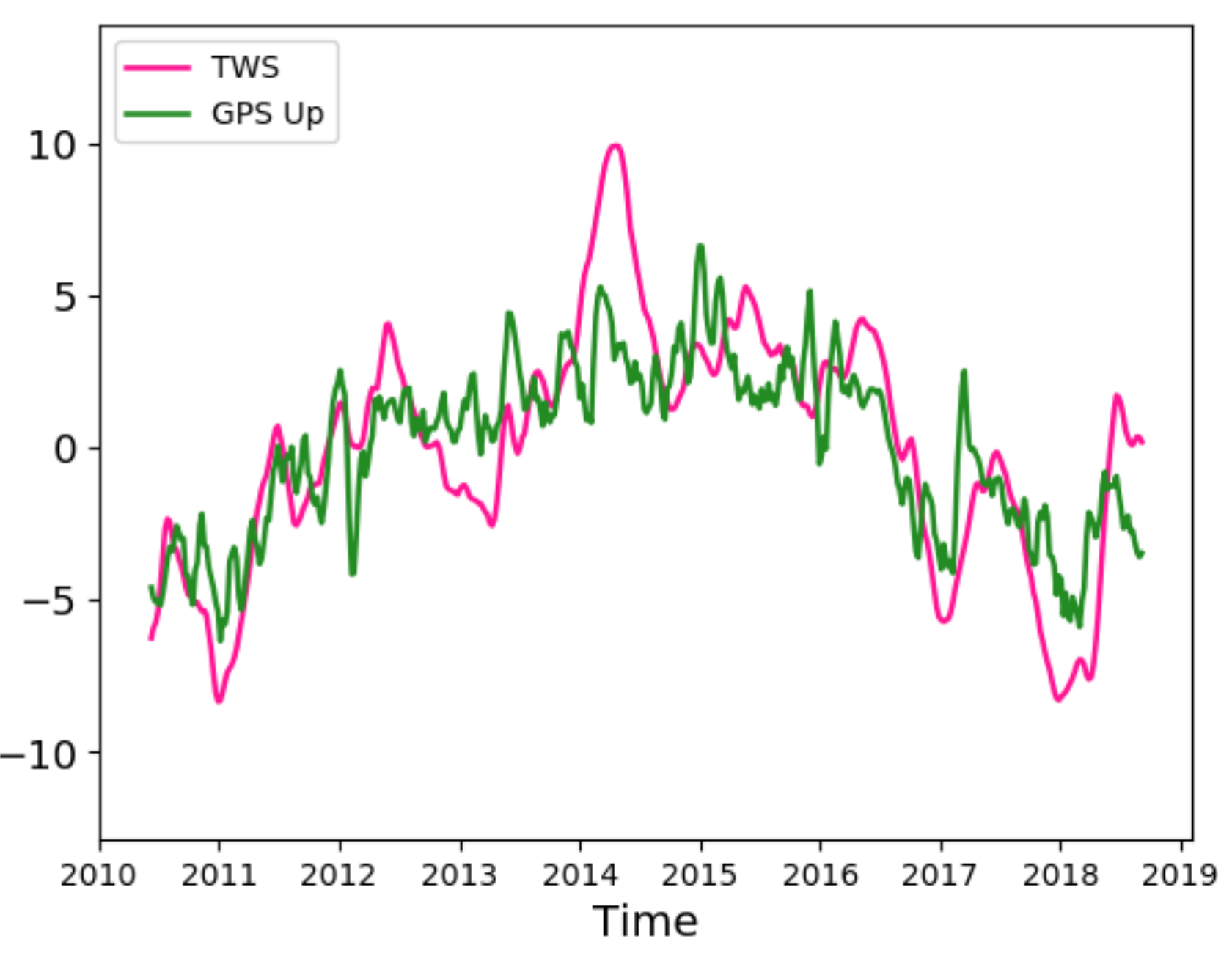
Figure 13 displays the first SVD time components, showing a 5-year period oscillation on which shorter-period variability is superimposed. We recall the detailed description of the climate-related effects provided in Section 3.1 concerning the Up, and Section 3.3 for the TWS. These effects can be recognized in this context as well. It is interesting to note that during 2014 and 2015 there is a phase shift between the relevant maxima and minima, while in the previous and following years this shift does not appear. During 2014, the Up increase anticipates by about two months the TWS decrease, while in 2015, the Up decrease follows the TWS increase by about three months.
The second coupled mode of variability explains 15% of total covariance. Figure 14a features the second spatial pattern of the TWS residuals, characterized by negative values in Eastern Europe, Baltic countries, Western Russia, and central-northern Scandinavia. Elsewhere, the coefficients are mostly slightly positive. Figure 14b shows the second spatial pattern of the Up coordinate exhibiting an opposite behavior with respect to that of the TWS, thus further supporting the idea of the loading effect on the Earth’s crust exerted by variations of the TWS. Figure 15 presents the second SVD time components, which are characterized by a parabolic variation (decadal period), with superimposed interannual fluctuations. Additionally, quite noticeable is the large fluctuation during the years 2016, 2017, and 2018, when climate warming caused record Northern Hemisphere average temperatures [55], and the European–Mediterranean area was affected by severe droughts. A long-period oscillation of similar shape does not appear in the SVD time components of the Up–SP pair, suggesting that the observed behavior is mostly due to the impact of the TWS.
5. GPS Up and Climate Indexes
Because in our study no significant correlations were found between the Up component and the AO, NAO, and EA indexes, in this section we only describe the correlation with the MEI.
We analyzed the correlation of the GPS Up residuals with the MEI because numerous studies have shed light on the association between precipitation in the European–Mediterranean region and the ENSO [56]. In order to reduce the potential effect of local anomalies, the GPS Up residuals were represented using the first two modes of variability, identified in Section 3.1. Since MEI is provided as a series of monthly values, monthly Up residuals were also estimated.
Figure 16 presents the monthly MEI time series made available by NOAA.
Figure 17 presents the standardized series of the MEI and those of the first (panel a) and second (panel b) PCA time components of the Up coordinate. The Up time components presented in this context were derived by a PCA analysis of the monthly Up time series. We observed significant (confidence level p < 0.05) correlations between the monthly time series of the MEI and those of the first and second time components of the GPS Up time series.
Over the whole period, MEI and the first time component are significantly anticorrelated (−0.23). However, if we account solely for the first four years (2010–2014), the two curves are positively correlated (+0.66). During this period, a strong La Niña event was active in 2010–2011, followed by a moderate event in 2011–2012, with decreasing strength until 2014. The following five years show a clear anticorrelation pattern. One of the most powerful El Niño events of the last few decades developed at the end of 2014; it lasted through middle 2016, followed by the warmest five-year period on record (2016–2020). The pattern described by the first time component suggests a fluctuation of about 5 years. A large deviation starting at the beginning of 2014 is noticeable when the transition from La Niña to a very strong El Niño event occurs. The second Up time component is well correlated (+0.58) with the MEI over an approximately decadal period.
Figure 18 shows the spatial distribution of the correlation coefficients between the MEI time series and those of the Up coordinate. The Up time series were reconstructed by means of the first two modes of variability (accounting for about 44% of total variance, see Table 1) of the PCA with the aim of avoiding possible disturbing signals induced by local effects. The grey dots identify those stations whose time series are not significantly correlated (p > 0.05) with MEI. The correlation map identifies two areas, one including Iberia, the Mediterranean, and Central and Northern Europe, where anticorrelation is clearly identifiable, and a second zone encompassing Scandinavia, Western Russia, and Baltic states, characterized by positive correlation.
6. Discussion
6.1. Interannual Vertical Deformations and Variations of SP and TWS
The Earth’s crust undergoes deformations of different nature. Recent studies have proposed methods to extract common mode components from GPS coordinates time series with the aim of identifying spatial and temporal patterns of certain signals [54,57]. Of increasing interest are signals related to climate variations/changes. Hence, it is important to identify interannual variations and examine their possible attribution. Vertical displacements induced by loading of the crust are explained for environmental parameters, such as the SP and TWS. Using a PCA approach and eight years of data (2010–2018) from a network of 114 GPS stations, we investigated the interannual variability of the vertical deformation over the European continent, including the Mediterranean area, in relation to fluctuations of the SP and TWS. Main modes of variability of the vertical component were identified through the PCA analysis, with the first two modes explaining 44.3% of the total (Table 1). The first mode shows a homogenous spatial behavior of Europe and the Mediterranean, with larger magnitudes of the coefficients around central-northern Europe and the Balkans. The behavior of the first time component, characterized by a 5-year period oscillation with maxima in 2012 and 2018 and minimum in 2015, can be explained in terms of loading variations, likely attributable to TWS. Evidence of this process is also provided by the result of the first SVD between the GPS Up and the TWS, which identifies two different spatially coherent behaviors—namely, that of Europe and the Mediterranean area in the center-south and Scandinavia, Baltic countries, and Western Russia in the north. The second time component reveals a decadal period suggesting Up decrease till about 2015, followed by increase in the south west of Europe, while the northeast shows an opposite pattern. The second SVD between the Up and the TWS substantiates this finding.
The SP loading effect on the crust is also noticeable. The first SVD space and time components between the GPS Up and the SP clearly indicate an opposite behavior of the two fields over the entire study area. The second SVD spatial pattern confirms the opposite behavior of Southern Europe and the Mediterranean with respect to the north.
The footprint of hydrological loading in GPS time series has been recognized. Another example is a study focusing on the Eastern Tibetan Plateau [58], which has shown interannual nonlinear signals in the common mode components of the GPS time series, predominantly related to hydrological loading.
6.2. MEI and Vertical Deformations
Several studies have underpinned the association between precipitation in the Mediterranean region and the ENSO. Shaman and Tziperman [56] have shown that interannual variability of fall and early winter (September–December) precipitation over Southwestern Europe (Iberia, Southern France, and Italy) is linked to ENSO variability in the eastern Pacific via an eastward-propagating stationary Rossby wave train. It has been documented [59] that, when El Niño is active, precipitation increases during late summer, autumn, and early winter in Western Europe and the Mediterranean region; however, during late winter and spring, the correlation is negative. The study also found spatially coherent patterns in Central and Eastern Europe, where the correlation is negative in autumn and positive during winter and spring. The outcomes of these studies corroborate our findings. In fact, the first time component of the TWS presented in Figure 7a shows precipitation increase in late summer, autumn, and early winter of 2014 and 2015. We recall that 2014 was characterized by the onset of a very strong El Niño that fully developed during 2015 and terminated in middle 2016. In Figure 17a, during the strong El Niño conditions, we observe anticorrelation between the MEI and the Up first time component during late summer and autumn of 2014 and early winter 2014–2015, while positive correlation is found during late winter and spring 2015. A similar pattern is recognizable during 2015–2016. This behavior can be explained with the loading/unloading process of the Earth’s crust exerted by the increase/absence of precipitation. The outcomes of the SVD analysis of the TWS and the GPS Up, described in Section 4.2, agree with these results, which is expected since precipitation is among the main contributors to TWS. The pattern of the first time component of the vertical deformation shows a nearly 5-year oscillation, with a well-recognizable change at the beginning of 2014, when switching from a period of about 4 years of strong first and then moderate La Niña to a very strong El Niño. Figure 7b illustrates an approximately decadal fluctuation of the second time component of the vertical deformation peaking in middle March 2015, about six months before El Niño reaches its maximum strength in middle October 2015. Timescales like the ones observed in this study were identified by Cheng and Ries [60] when analyzing four decades of significant variations in the Earth’s dynamical oblateness (J2) derived from satellite laser ranging data. They explain a timescale of ~2~6 years by the mass redistribution in the atmosphere and ocean associated with the ENSO events during the period from 1998 to 2016. The significant oscillation they find at ~10.4 timescale can be described by existing models of atmosphere, ocean, and surface water changes only up to the level of ~18%. However, they suggest that the observed decadal variation is a consequence of mass redistribution within atmosphere–ocean-hydrosphere associated with ENSO events since the observed variation is well correlated with a 5-year running mean of the ENSO index. Additionally, Chao et al. [61] investigated the variation of the Earth’s oblateness J2 on interannual-to-decadal timescales. They indicate contributions from the Antarctic Oscillation (AAO) and the AO for time scale shorter than 5 years and from the Pacific Decadal Oscillation (PDO) for timescale longer than 5 years. According to their findings, contributions from ENSO and the Atlantic Multidecadal Oscillation (AMO) are absent. For the 10.5-year signal, they suggest a non-climatic origin—namely, the solar cycle, although this apparent correlation is presently uncertain.
7. Conclusions
The time series of the vertical movements of the Earth’s crust contain signals due to the evolution of geophysical and climatic processes. This study shows evidence, over Europe and the Mediterranean area, of interannual and longer period variability of GPS-derived vertical deformations and of their relationship with the spatial and temporal variability of environmental parameters, such as TWS, SP, and the MEI climate index. The GPS heights and the environmental parameters data series were analyzed using a PCA approach, further correlated by means of the SVD technique. The first two modes of variability of the height were also correlated with the MEI index.
The first and second time component of the height residuals, responsible for more than 44% of the observed variance, show a 5-year and a decadal variation (9 years is the time frame of this study), respectively. Both curves exhibit superimposed shorter period variability. Over the 5-year timescale, the whole of Europe and the Mediterranean behave coherently, with Central Europe and the Balkans denoted by larger coefficients. The spatial pattern of the decadal fluctuation presents a north–south gradient. The observed height variations are explained in terms of loading variations on the Earth’s crust, likely associated for the 5-year periodicity with the transition from a few years of strong and moderate La Niña to a very strong El Niño and to a sequence of severe droughts that affected the study area during 2010–2012 and again during 2015–2018. The decadal timescale can be related to the occurrence of the strong ENSO event and the associated hydroclimate anomalies that are generally characterized, in the European–Mediterranean area, by a north–south path. The retrieved pattern is compatible, in fact, with positive precipitation anomaly in Scandinavia and negative anomaly in Southern Europe related to a strong La Niña event (2010–2011), followed by a moderate event (2011–2012) weakening until the beginning of 2015 when a strong El Niño started lasting about one and one-half years. This last period was characterized by negative precipitation anomaly in Scandinavia and positive anomaly in Southern Europe. The short-period variations superimposed to both the 5-year and to the decadal period are related to specific weather and climate events.
The spatial patterns found for the SP and the TWS time series are in good agreement with those of the height by showing for the first mode a coherent behavior of the study area and a north–south gradient for the second mode, which is particularly clear for the SP series. As for the TWS, coefficients of larger magnitude are present in Central Europe. A periodicity of about 2 years can be recognized in the first time component, while a decadal timescale shows up in the second.
The SVD analysis between height and SP has clearly identified the anticorrelation between these two parameters, which is explained by the loading response of the crust to SP variations. The results also elucidate the different response, to the same SP forcing, of inland and coastal sites, with the former showing larger effects. A 5-year timescale is present in the SVD first time component. We observe a north–south gradient in the second spatial component; however, the relevant time behavior does not present any identifiable long-period feature.
The coupled variability of height and TWS shows clear anticorrelation, explained by the loading mechanism. The study area is not coherent since an opposite behavior between north and south is observed. A 5-year oscillation can be recognized in the first SVD mode. The second mode of coupled variability, also showing anticorrelation, exhibits a nearly decadal variation which was not found in the SVD results of the pair height and SP. This suggests that the observed decadal variation of the height is due to the TWS variations rather than to those of SP.
The comparison between the MEI index and the stations’ height, represented by the first two modes of a monthly PCA analysis, shows quite a coherent pattern of anticorrelation in the large area encompassing Iberia, the Mediterranean, and central-northern Europe. Instead, more to the north, the region comprising Scandinavia, Baltic countries, and Western Russia is positively correlated. The comparison between the first and second time components and MEI sheds light on the height interannual variability due to climatic fluctuations—namely, those that may be associated with the ENSO phenomenon. The 5-year fluctuation present in the first time component is likely modulated by the sequence of a strong and a moderate La Niña, followed by the strongest El Niño of the last two decades. The large oscillations that characterize the years 2016, 2017, and 2018 are realistically due to the severe droughts that affected the study area. The decadal oscillation shaping the second height time component is well correlated with the MEI index behavior. The correlation is significant, p < 0.05, with a value of +0.58. Iberia, central-northern Europe, and the Mediterranean area experience height decrease till about the onset of the strong 2015–2016 El Niño event, followed by increase during the subsequent four years. The opposite behavior characterizes Scandinavia, the Baltic countries, and Western Russia.
Author Contributions
L.E., F.R., S.Z. Individual contributions are according to the following statements: Conceptualization, S.Z., L.E. and F.R.; methodology, S.Z., L.E. and F.R.; software, L.E.; validation, S.Z., L.E. and F.R.; formal analysis, L.E.; investigation, L.E., S.Z. and F.R.; resources S.Z.; data curation, L.E.; writing S.Z., L.E. and F.R.; writing—review and editing, S.Z., L.E. and F.R.; visualization, L.E.; supervision, S.Z.; project administration, S.Z.; funding acquisition, S.Z. All authors have read and agreed to the published version of the manuscript.
Funding
This research was funded by the University of Bologna, grant ECOCZERB and The APC was funded by grant ECOCZERB.
Institutional Review Board Statement
Not applicable.
Informed Consent Statement
Not applicable.
Data Availability Statement
The data presented in this study are available on request from the corresponding author.
Acknowledgments
This research was funded by the University of Bologna, grant ECOCZERB.
Conflicts of Interest
The authors declare no conflict of interest.
References
- Teixell, A.; Bertotti, G.; Frizon de Lamotte, D.; Charroud, M. The geology of vertical movements of the lithosphere: An overview. Tectonophysics 2009, 475, 1–8. [Google Scholar] [CrossRef]
- Blewitt, G.; Lavallée, D.; Clarke, P.; Nurutdinov, K. A New Global Mode of Earth Deformation: Seasonal Cycle Detected. Science 2001, 294, 2342–2345. [Google Scholar] [CrossRef] [PubMed] [Green Version]
- Blewitt, G.; Lavallée, D. Effect of annual signals on geodetic velocity. J. Geophys. Res. Solid Earth 2002, 107, ETG 9-1–ETG 9-11. [Google Scholar] [CrossRef] [Green Version]
- Blewitt, G.; Lavallée, D. Correction to “Effect of annual signals on geodetic velocity” by Geoffrey Blewitt and David Lavallée. J. Geophys. Res. Solid Earth 2003, 108, ETG 4-1. [Google Scholar] [CrossRef]
- Farrell, W.E. Deformation of the Earth by surface loads. Rev. Geophys. 1972, 10, 761–797. [Google Scholar] [CrossRef]
- Van Dam, T.M.; Wahr, J. Modeling environment loading effects: A review. Phys. Chem. Earth 1998, 23, 1077–1087. [Google Scholar] [CrossRef]
- Gegout, P.; Boy, J.-P.; Hinderer, J.; Ferhat, G. Modeling and Observation of Loading Contribution to Time-Variable GPS Sites Positions. In Gravity, Geoid and Earth Observation; Mertikas, S., Ed.; Springer: Berlin/Heidelberg, Germany, 2010; Volume 135, pp. 651–659. [Google Scholar] [CrossRef]
- Petrov, L.; Boy, J.-P. Study of the atmospheric pressure loading signal in very long baseline interferometry observations. J. Geophys. Res. Solid Earth 2004, 109, B03405. [Google Scholar] [CrossRef] [Green Version]
- Tregoning, P.; Van Dam, T.M. Atmospheric pressure loading corrections applied to GPS data at the observation level. Geophys. Res. Lett. 2005, 32, L22310. [Google Scholar] [CrossRef] [Green Version]
- Girotto, M.; Rodell, M. Chapter Two—Terrestrial water storage. In Extreme Hydroclimatic Events and Multivariate Hazards in a Changing Environment; Maggioni, V., Massari, C., Eds.; Elsevier: Amsterdam, The Netherlands, 2019; pp. 41–64. [Google Scholar] [CrossRef] [Green Version]
- Van Dam, T.; Lavallée, D.; Wahr, J.; Milly, C.D.; Shmakin, A.B.; Blewitt, G.; Larson, K.M. Crustal displacements due to continental water loading. Geophys. Res. Lett. 2001, 28, 651–654. [Google Scholar] [CrossRef] [Green Version]
- Subirana, J.S.; Zornoza, J.M.J.; Hernández-Pajares, M. Earth Deformation Effects Modelling. In GNSS Data Processing, Vol. I: Fundamentals and Algorithms; Fletcher, K., Ed.; ESA Communications ESTEC: Noordwijk, The Netherlands, 2013; Volume 1, pp. 134–137. ISSN 1013-7076. Available online: https://gssc.esa.int/navipedia/GNSS_Book/ESA_GNSS-Book_TM-23_Vol_I.pdf (accessed on 28 October 2020).
- Zerbini, S.; Matonti, F.; Raicich, F.; Richter, B.; van Dam, T. Observing and assessing nontidal ocean loading using ocean, continuous GPS and gravity data in the Adriatic area. Geophys. Res. Lett. 2004, 31, L23609. [Google Scholar] [CrossRef]
- van Dam, T.; Collilieux, X.; Wuite, J.; Altamimi, Z.; Ray, J. Nontidal ocean loading: Amplitudes and potential effects in GPS height time series. J. Geod. 2012, 86, 1043–1057. [Google Scholar] [CrossRef] [Green Version]
- Mémin, A.; Boy, J.-P.; Santamaría-Gómez, A. Correcting GPS measurements for non-tidal loading. GPS Solut. 2020, 24, 45. [Google Scholar] [CrossRef]
- Wu, S.; Nie, G.; Meng, X.; Liu, J.; He, Y.; Xue, C.; Li, H. Comparative Analysis of the Effect of the Loading Series from GFZ and EOST on Long-Term GPS Height Time Series. Remote Sens. 2020, 12, 2822. [Google Scholar] [CrossRef]
- Kaczmarek, A. Influence of Geophysical signals on coordinate variations GNSS permanent stations in central Europe. Artif. Satell. 2019, 54, 57–71. [Google Scholar] [CrossRef] [Green Version]
- Li, Z.; Chen, W.; van Dam, T.; Reibischung, P.; Altamimi, Z. Comparative analysis of different atmospheric surface pressure models and their impacts on daily ITRF2014 GNSS residual time series. J. Geod. 2020, 94, 42. [Google Scholar] [CrossRef]
- Ostanciaux, E.; Husson, L.; Choblet, G.; Robin, C.; Pedoja, K. Present-day trends of vertical ground motion along the coast lines. Earth Sci. Rev. 2012, 110, 74–92. [Google Scholar] [CrossRef] [Green Version]
- Springer, A.; Karegar, M.A.; Kusche, J.; Keune, J.; Kurtz, W.; Kollet, S. Evidence of daily hydrological loading in GPS time series over Europe. J. Geod. 2019, 93, 2145–2153. [Google Scholar] [CrossRef]
- Tiwari, V.M.; Srinivas, N.; Singh, B. Hydrological changes and vertical crustal deformation in south India: Inference from GRACE, GPS and absolute gravity data. Phys. Earth Planet. Int. 2014, 231, 74–80. [Google Scholar] [CrossRef]
- Jin, S.; Zhang, T. Terrestrial Water Storage Anomalies Associated with Drought in Southwestern USA from GPS Observations. Surv. Geophys. 2016, 37, 1139–1156. [Google Scholar] [CrossRef]
- Adusumilli, S.; Borsa, A.A.; Fish, M.A.; McMillan, H.K.; Silverii, F. A decade of Water Storage Changes across the Contiguous United States from GPS and Satellite Gravity. Geophys. Res. Lett. 2019, 46, 13006–13015. [Google Scholar] [CrossRef]
- Compton, K.; Bennett, R.A.; Hreinsdóttir, S. Climate-driven vertical acceleration of Icelandic crust measured by continuous GPS geodesy. Geophys. Res. Lett. 2015, 42, 743–750. [Google Scholar] [CrossRef]
- Zerbini, S.; Raicich, F.; Errico, M.; Cappello, G. An EOF and SVD analysis of interannual variability of GPS coordinates, environmental parameters and space gravity data. J. Geodyn. 2013, 67, 111–124. [Google Scholar] [CrossRef]
- Blewitt, G.; Hammond, W.C.; Kreemer, C. Harnessing the GPS Data Explosion for Interdisciplinary Science. Eos 2018, 99. [Google Scholar] [CrossRef]
- SOPAC. The Scripps Orbit and Permanent Array Center. Available online: http://sopac.ucsd.edu/ (accessed on 18 June 2020).
- Bruni, S.; Zerbini, S.; Raicich, F.; Errico, M.; Santi, E. Detecting discontinuities in GNSS coordinate time series with STARS: Case study, the Bologna and Medicina GPS sites. J. Geod. 2014, 88, 1203–1214. [Google Scholar] [CrossRef]
- Kalnay, E.; Kanamitsu, M.; Kistler, R.; Collins, W.; Deaven, D.; Gandin, L.; Iredell, M.; Saha, S.; White, G.; Woollen, J.; et al. The NCEP/NCAR 40-year reanalysis project. Bull. Amer. Meteor. Soc. 1996, 77, 437–470. [Google Scholar] [CrossRef] [Green Version]
- Global Modeling and Assimilation Office (GMAO). MERRA-2 tavg1_2d_lnd_Nx: 2d,1-Hourly, Time-Averaged, Single-Level, Assimilation, Land Surface Diagnostics V5.12.4, Greenbelt, MD, USA, Goddard Earth Sciences Data and Information Services Center (GES DISC), 2015. Available online: https://arcticdata.io/catalog/view/doi%3A10.18739%2FA27M0416J (accessed on 30 September 2020). [CrossRef]
- Jolliffe, I.T.; Cadima, J. Principal component analysis: A review and recent developments. Phil. Trans. R. Soc. A 2016, 374, 20150202. [Google Scholar] [CrossRef]
- Papoulis, A. A new algorithm in spectral analysis and band-limited extrapolation. IEEE Trans. Circuits Syst. 1975, 22, 735–742. [Google Scholar] [CrossRef]
- Gerchberg, R. Super-resolution through error energy reduction. Opt. Acta 1974, 21, 709–720. [Google Scholar] [CrossRef]
- Roweis, S. EM algorithms for PCA and SPCA. In Advances in Neural Information Processing Systems; MIT Press: Cambridge, MA, USA, 1998; Volume 10, pp. 626–632. [Google Scholar]
- Björnsson, H.; Venegas, S. A Manual for EOF and SVD Analyses of Climatic Data. McGill Univ. Rep. N 1997, 97, 112–134. Available online: http://www.geog.mcgill.ca/gec3/wp-content/uploads/2009/03/Report-no.-1997-1.pdf (accessed on 4 May 2020).
- GCOS. Available online: https://gcos.wmo.int/en/essential-climate-variables (accessed on 22 January 2020).
- WMO. Statement on the State of the Global Climate in 2011; World Meteorological Organization: Geneva, Switzerland, 2012; No 1085; p. 19. ISBN 978-92-63-11085-5. Available online: https://library.wmo.int/index.php?lvl=notice_display&id=9754#.YBLB9-hKhjk (accessed on 14 January 2021).
- Bissolli, P.; Ziese, M.; Pietzsch, S.; Finger, P.; Friedrich, K.; Nitsche, H.; Obregón, A. Drought conditions in Europe in the spring of 2012. Dtsch. Wetterd. 2012. Available online: https://www.dwd.de/EN/ourservices/specialevents/drought/20120810_Trockenheit_2012_en.pdf?_blob=publicationFile&v=4 (accessed on 13 January 2021).
- WMO. Statement on the State of the Global Climate in 2013; World Meteorological Organization: Geneva, Switzerland, 2014; No 1130; Volume 21, ISBN 978-92-63-11130-2. Available online: https://library.wmo.int/index.php?lvl=notice_display&id=15957#.YBLBq-hKhjk (accessed on 14 January 2021).
- WMO. Statement on the State of the Global Climate in 2014; World Meteorological Organization: Geneva, Switzerland, 2015; No 1152; Volume 19, ISBN 978-92-63-11152-4. Available online: https://library.wmo.int/index.php?lvl=notice_display&id=16898#.YBLVeehKhjk (accessed on 14 January 2021).
- WMO. Statement on the State of the Global Climate in 2015; World Meteorological Organization: Geneva, Switzerland, 2016; No 1167; Volume 23, ISBN 978-92-63-11167-8. Available online: https://library.wmo.int/index.php?lvl=notice_display&id=19125#.YBLDkOhKhjk (accessed on 14 January 2021).
- Ionita, M.; Tallaksen, L.M.; Kingstone, D.G.; Stagge, J.H.; Laaha, G.; Van Lanen, H.A.J.; Scholz, P.; Chelcea, S.M.; Haslinger, K. The European 2015 drought from a climatological perspective. Hydrol. Earth Syst. Sci. 2017, 21, 1397–1419. [Google Scholar] [CrossRef] [Green Version]
- García-Herrera, R.; Garrido-Perez, J.M.; Barriopedro, D.; Ordóñez, C.; Vicente-Serrano, S.M.; Nieto, R.; Gimeno, L.; Sorí, R.; Yiou, P. The European 2016/17 Drought. J. Clim. 2019, 32, 3169–3187. [Google Scholar] [CrossRef]
- WMO. Statement on the State of the Global Climate in 2017; World Meteorological Organization: Geneva, Switzerland, 2018; No 1212; Volume 35, ISBN 978-92-63-11212-5. Available online: https://library.wmo.int/index.php?lvl=notice_display&id=20220#.YBLgL-hKhjk (accessed on 15 January 2021).
- Copernicus. Climate in 2017—European Wet and Dry Indicators. Available online: https://climate.copernicus.eu/climate-2017-european-wet-and-dry-indicators (accessed on 11 February 2021).
- WMO. Statement on the State of the Global Climate in 2018; World Meteorological Organization: Geneva, Switzerland, 2019; No 1233; Volume 39, ISBN 978-92-63-11233-0. Available online: https://library.wmo.int/index.php?lvl=notice_display&id=20799#.YBPg5-hKhjk (accessed on 15 January 2021).
- King, M.P.; Yu, E.; Sillmann, J. Impact of strong and extreme El Niños on European hydroclimate. Tellus A 2020, 72, 1–10. [Google Scholar] [CrossRef] [Green Version]
- Brönnimann, S.; Xoplaki, E.; Casty, C.; Pauling, A.; Luterbacher, J. ENSO influence on Europe during the last centuries. Clim. Dyn. 2007, 28, 181–197. [Google Scholar] [CrossRef] [Green Version]
- Roesli, H.-P. A Westward Travelling ULL Induced the Rapid Reversal of a Pressure Gradient across the Alpine Range in Mid-March 2016. Last Updated 4 November 2020. Available online: http://eumetsat.int/upper-level-low-ull-over-northern-europe (accessed on 12 February 2021).
- WMO. Statement on the State of the Global Climate in 2010; World Meteorological Organization: Geneva, Switzerland, 2011; No 1074; Volume 15, ISBN 978-92-63-11074-9. Available online: https://library.wmo.int/doc_num.php?explnum_id=7739 (accessed on 22 January 2021).
- WMO. Statement on the State of the Global Climate in 2012; World Meteorological Organization: Geneva, Switzerland, 2013; No 1108; p. 33. ISBN 978-92-63-11108-1. Available online: https://library.wmo.int/index.php?lvl=notice_display&id=14750#.YBP0s-hKhjk (accessed on 15 January 2021).
- WMO. Statement on the State of the Global Climate in 2016; World Meteorological Organization: Geneva, Switzerland, 2017; No 1189; Volume 23, ISBN 978-92-63-11189-0. Available online: https://library.wmo.int/index.php?lvl=notice_display&id=19835#.YBP9VOhKhjk (accessed on 15 January 2021).
- van Dam, T.M.; Blewitt, G.; Heflin, M.B. Atmospheric pressure loading effects on Global Positioning System coordinate determinations. J. Geophys. Res. 1994, 99, 23939–23950. [Google Scholar] [CrossRef]
- Kreemer, C.; Blewitt, G. Robust estimation of spatially varying common-mode components in GPS time-series. J. Geod. 2021, 95, 13. [Google Scholar] [CrossRef]
- Wouter, P.; Bastos, A.; Ciais, P.; Vermeulen, A. A Historical, geographical and ecological perspective on the 2018 summer drought. Phil. Trans. R. Soc. B 2020, 375, 20190505. [Google Scholar] [CrossRef]
- Shaman, J.; Tziperman, E. An Atmospheric Teleconnection Linking ENSO and Southwestrn European Precipitation. J. Clim. 2011, 24, 124–139. [Google Scholar] [CrossRef] [Green Version]
- Tian, Y.; Shen, Z.-K. Extracting the regional common-mode component O GPS station position time series from dense continuous network. J. Geophys. Res. Solid Earth 2016, 121, 1080–1096. [Google Scholar] [CrossRef]
- Pan, Y.; Chen, R.; Ding, H.; Xu, X.; Zheng, G.; Shen, W.; Xiao, I. Common Mode Component and Its Potential Effect on GPS-Inferred Three-Dimensional Crustal Deformations in the Eastern Tibetan Plateau. Remote Sens. 2019, 11, 1975. [Google Scholar] [CrossRef] [Green Version]
- Mariotti, A.; Zeng, N.; Lau, K.-M. Euro Mediterranean rainfall and ENSO—A seasonally varying relationship. Geophys. Res. Lett. 2002, 29, 1621. [Google Scholar] [CrossRef] [Green Version]
- Cheng, M.; Ries, J.C. Decadal variation in Earth’s oblateness (J2) from satellite laser ranging data. Geophys. J. Int. 2018, 212, 1218–1224. [Google Scholar] [CrossRef]
- Chao, B.F.; Yu, Y.; Chung, C.H. Variation of Earth’s Oblateness J2 on Interannual-to-Decadal Timescales. J. Geophys. Res. Solid Earth 2020, 125, e2020JB019421. [Google Scholar] [CrossRef]
Figure 1.
Location of the GPS stations selected for this work.

Figure 2.
First (a) and second (b) spatial pattern of the weekly GPS Up coordinate residuals.

Figure 3.
First (a) and second (b) time component of the weekly GPS Up coordinate residuals.

Figure 4.
First (a) and second (b) spatial pattern of the weekly SP residuals.

Figure 5.
First (a) and second (b) time component of the weekly SP residuals.

Figure 6.
First (a) and second (b) spatial pattern of the weekly TWS residuals.

Figure 7.
First (a) and second (b) time component of the weekly TWS residuals.

Figure 8.
Spatial pattern coefficients describing the first single-value decomposition (SVD) of the residuals of the SP and of those of the Up coordinate. (a) SP spatial pattern; (b) Up spatial pattern.
Figure 8.
Spatial pattern coefficients describing the first single-value decomposition (SVD) of the residuals of the SP and of those of the Up coordinate. (a) SP spatial pattern; (b) Up spatial pattern.

Figure 9.
Time components of the first SVD of the residuals of the variable pair (monthly values) SP (magenta line) and Up coordinate (green line).
Figure 9.
Time components of the first SVD of the residuals of the variable pair (monthly values) SP (magenta line) and Up coordinate (green line).

Figure 10.
Spatial pattern coefficients describing the second SVD of the residuals of the SP and those of the Up coordinate. (a) SP spatial pattern; (b) Up spatial pattern.
Figure 10.
Spatial pattern coefficients describing the second SVD of the residuals of the SP and those of the Up coordinate. (a) SP spatial pattern; (b) Up spatial pattern.

Figure 11.
Time components of the second SVD of the residuals of the variable pair (monthly values) SP (magenta line) and Up coordinate (green line).
Figure 11.
Time components of the second SVD of the residuals of the variable pair (monthly values) SP (magenta line) and Up coordinate (green line).

Figure 12.
Spatial pattern coefficients describing the first SVD of the residuals of the TWS and those of the Up coordinate. (a) TWS spatial pattern; (b) Up spatial pattern.
Figure 12.
Spatial pattern coefficients describing the first SVD of the residuals of the TWS and those of the Up coordinate. (a) TWS spatial pattern; (b) Up spatial pattern.

Figure 13.
Time components of the first SVD of the residuals of the variable pair (monthly values) TWS (magenta line) and Up coordinate (green line).
Figure 13.
Time components of the first SVD of the residuals of the variable pair (monthly values) TWS (magenta line) and Up coordinate (green line).

Figure 14.
Spatial pattern coefficients describing the second SVD of the residuals of the TWS and those of the Up coordinate. (a) TWS spatial pattern; (b) Up spatial pattern.
Figure 14.
Spatial pattern coefficients describing the second SVD of the residuals of the TWS and those of the Up coordinate. (a) TWS spatial pattern; (b) Up spatial pattern.

Figure 15.
Time components of the second SVD of the residuals of the variable pair (monthly values) TWS (magenta line) and Up coordinate (green line).
Figure 15.
Time components of the second SVD of the residuals of the variable pair (monthly values) TWS (magenta line) and Up coordinate (green line).

Figure 16.
Time series of the multivariate El Niño Southern Oscillation (ENSO) index (MEI)v2. The red color represents the warm phase (El Niño) while the blue color indicates the cold phase (La Niña). Image downloaded from https://psl.noaa.gov/enso/mei/, accessed on 20 January 2021.
Figure 16.
Time series of the multivariate El Niño Southern Oscillation (ENSO) index (MEI)v2. The red color represents the warm phase (El Niño) while the blue color indicates the cold phase (La Niña). Image downloaded from https://psl.noaa.gov/enso/mei/, accessed on 20 January 2021.

Figure 17.
Standardized monthly time series of the MEI (purple line) and of the first (a) and second (b) PCA time components of the Up coordinate.
Figure 17.
Standardized monthly time series of the MEI (purple line) and of the first (a) and second (b) PCA time components of the Up coordinate.

Figure 18.
Spatial distribution of the correlation coefficients between the MEI and the Up coordinate time series. The Up time series were generated by using the first two components of the PCA. The grey dots represent those stations whose time series are not significantly correlated with the MEI.
Figure 18.
Spatial distribution of the correlation coefficients between the MEI and the Up coordinate time series. The Up time series were generated by using the first two components of the PCA. The grey dots represent those stations whose time series are not significantly correlated with the MEI.


Table 1.
Percentage of variance explained by the first four modes of variability of the GPS Up coordinate residuals.
Table 1.
Percentage of variance explained by the first four modes of variability of the GPS Up coordinate residuals.
| Modes | Variance (%) |
|---|---|
| 1 | 32.77 |
| 2 | 11.55 |
| 3 | 5.58 |
| 4 | 4.13 |
Table 2.
Percentage of variance explained by the first four modes of variability of the surface pressure (SP) residuals.
Table 2.
Percentage of variance explained by the first four modes of variability of the surface pressure (SP) residuals.
| Modes | Variance (%) |
|---|---|
| 1 | 46.54 |
| 2 | 22.22 |
| 3 | 11.82 |
| 4 | 5.64 |
Table 3.
Percentage of variance explained by the first four modes of variability of the terrestrial water storage (TWS) residuals. Before being analyzed with the PCA methodology, the TWS time series were detrended, deseasonalized, and finally standardized.
Table 3.
Percentage of variance explained by the first four modes of variability of the terrestrial water storage (TWS) residuals. Before being analyzed with the PCA methodology, the TWS time series were detrended, deseasonalized, and finally standardized.
| Modes | Variance (%) |
|---|---|
| 1 | 29.67 |
| 2 | 12.08 |
| 3 | 10.39 |
| 4 | 7.78 |
Table 4.
Percentage of squared covariance explained by the first four modes of variability of the residuals of the pair Up–SP.
Table 4.
Percentage of squared covariance explained by the first four modes of variability of the residuals of the pair Up–SP.
| Modes | Squared Covariance (%) |
|---|---|
| 1 | 52.03 |
| 2 | 19.43 |
| 3 | 8.70 |
| 4 | 4.33 |
Table 5.
Percentage of squared covariance explained by the first four modes of variability of the residuals of the pair Up–TWS.
Table 5.
Percentage of squared covariance explained by the first four modes of variability of the residuals of the pair Up–TWS.
| Modes | Squared Covariance (%) |
|---|---|
| 1 | 20.20 |
| 2 | 14.98 |
| 3 | 9.35 |
| 4 | 6.30 |
Publisher’s Note: MDPI stays neutral with regard to jurisdictional claims in published maps and institutional affiliations. |
© 2021 by the authors. Licensee MDPI, Basel, Switzerland. This article is an open access article distributed under the terms and conditions of the Creative Commons Attribution (CC BY) license (https://creativecommons.org/licenses/by/4.0/).
Share and Cite
MDPI and ACS Style
Elia, L.; Zerbini, S.; Raicich, F. Interannual Variability of GPS Heights and Environmental Parameters over Europe and the Mediterranean Area. Remote Sens. 2021, 13, 1554. https://0-doi-org.brum.beds.ac.uk/10.3390/rs13081554
AMA Style
Elia L, Zerbini S, Raicich F. Interannual Variability of GPS Heights and Environmental Parameters over Europe and the Mediterranean Area. Remote Sensing. 2021; 13(8):1554. https://0-doi-org.brum.beds.ac.uk/10.3390/rs13081554
Chicago/Turabian StyleElia, Letizia, Susanna Zerbini, and Fabio Raicich. 2021. "Interannual Variability of GPS Heights and Environmental Parameters over Europe and the Mediterranean Area" Remote Sensing 13, no. 8: 1554. https://0-doi-org.brum.beds.ac.uk/10.3390/rs13081554
Note that from the first issue of 2016, this journal uses article numbers instead of page numbers. See further details here.