Joint Interpretation of Geophysical Results and Geological Observations for Detecting Buried Active Faults: The Case of the “Il Lago” Plain (Pettoranello del Molise, Italy)

 ,
,  ,
,  , , ,
, , ,  and
and
Abstract
:1. Introduction
2. Geological and Seismological Context
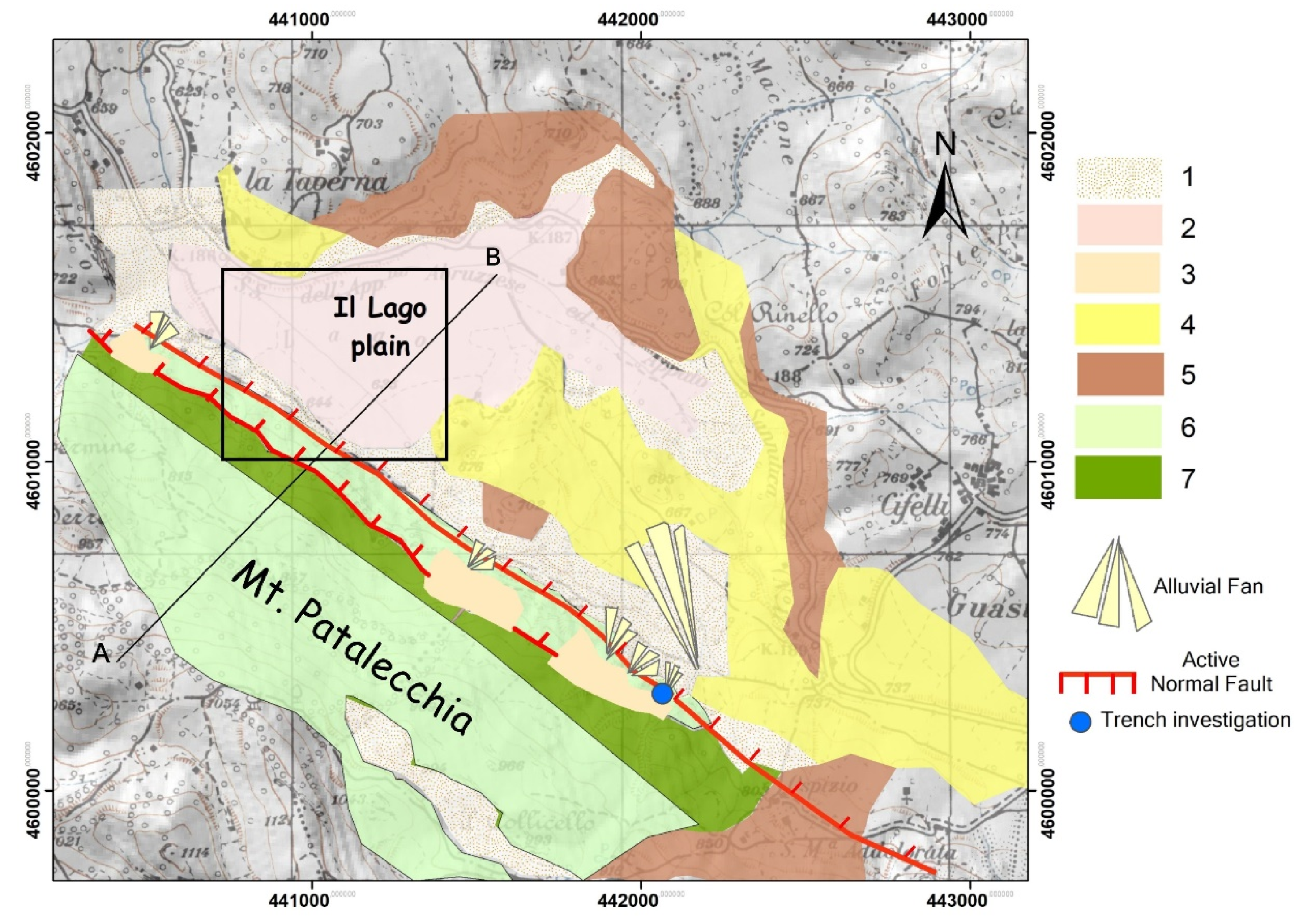
2.1. Regional Setting
2.2. The Bojano Basin Fault-System
2.3. Paleoseismicity and Historical Seismicity
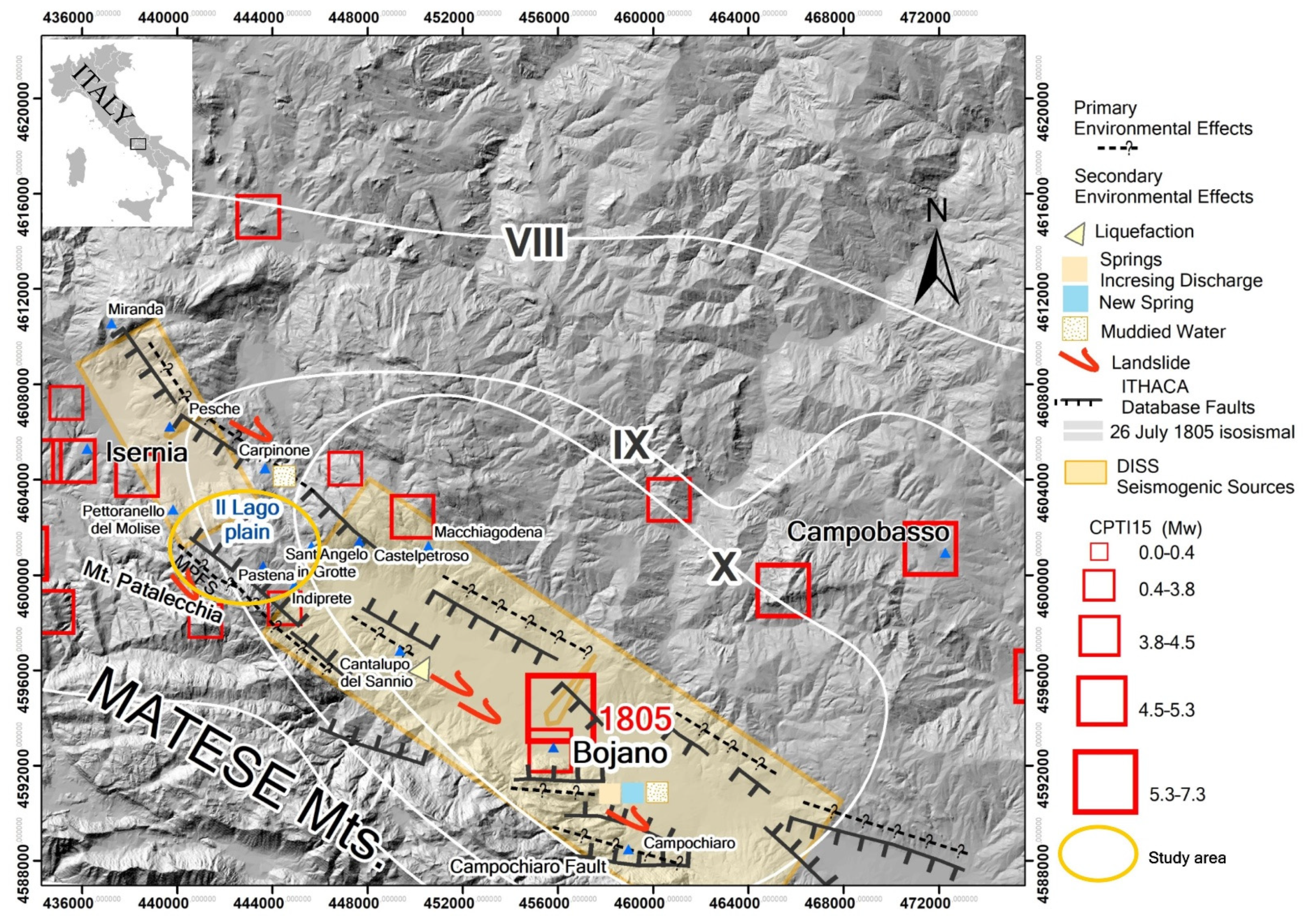
2.4. Environmental Effects of the 1805 S. Anna’s Earthquake
3. Data and Methods
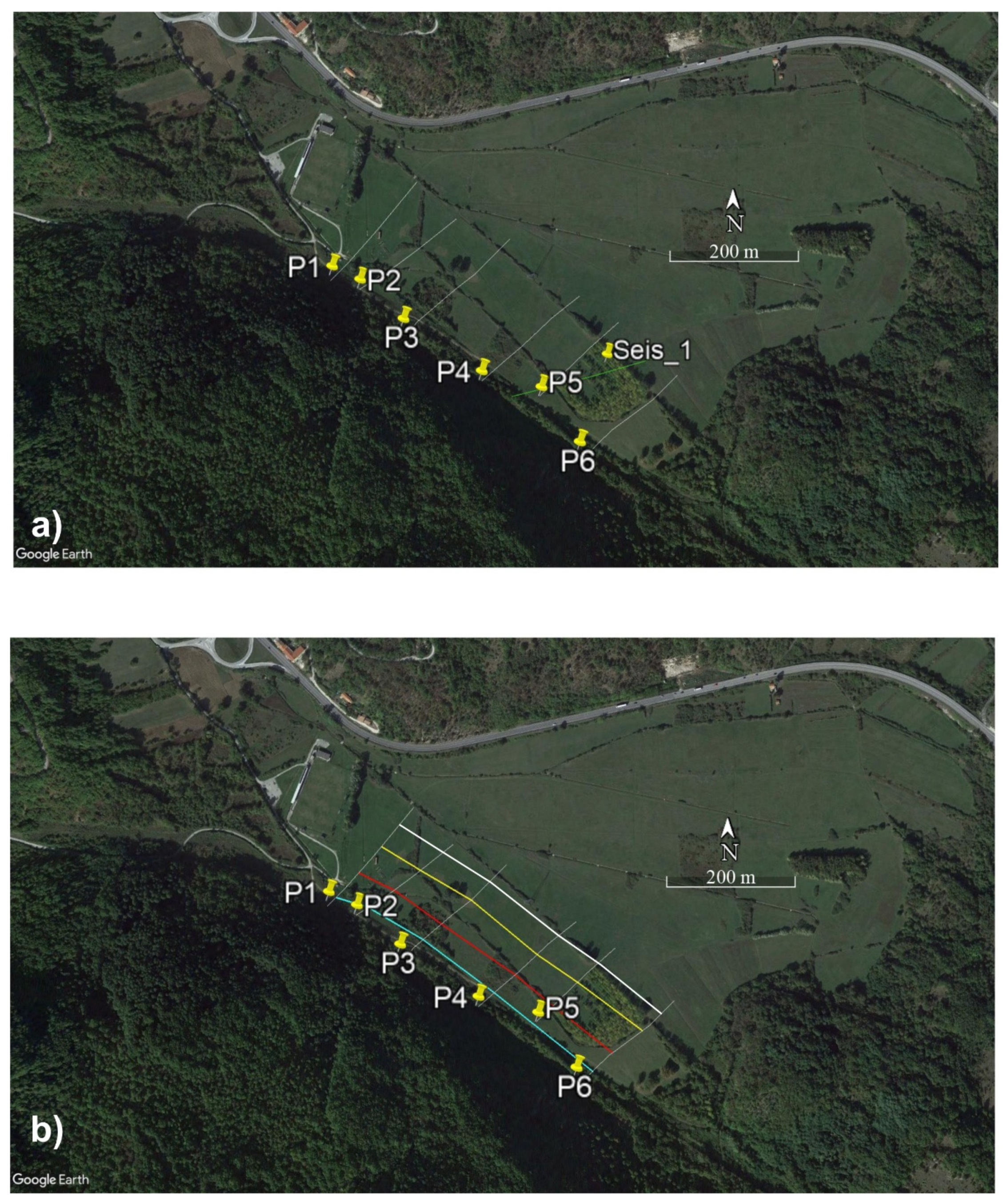
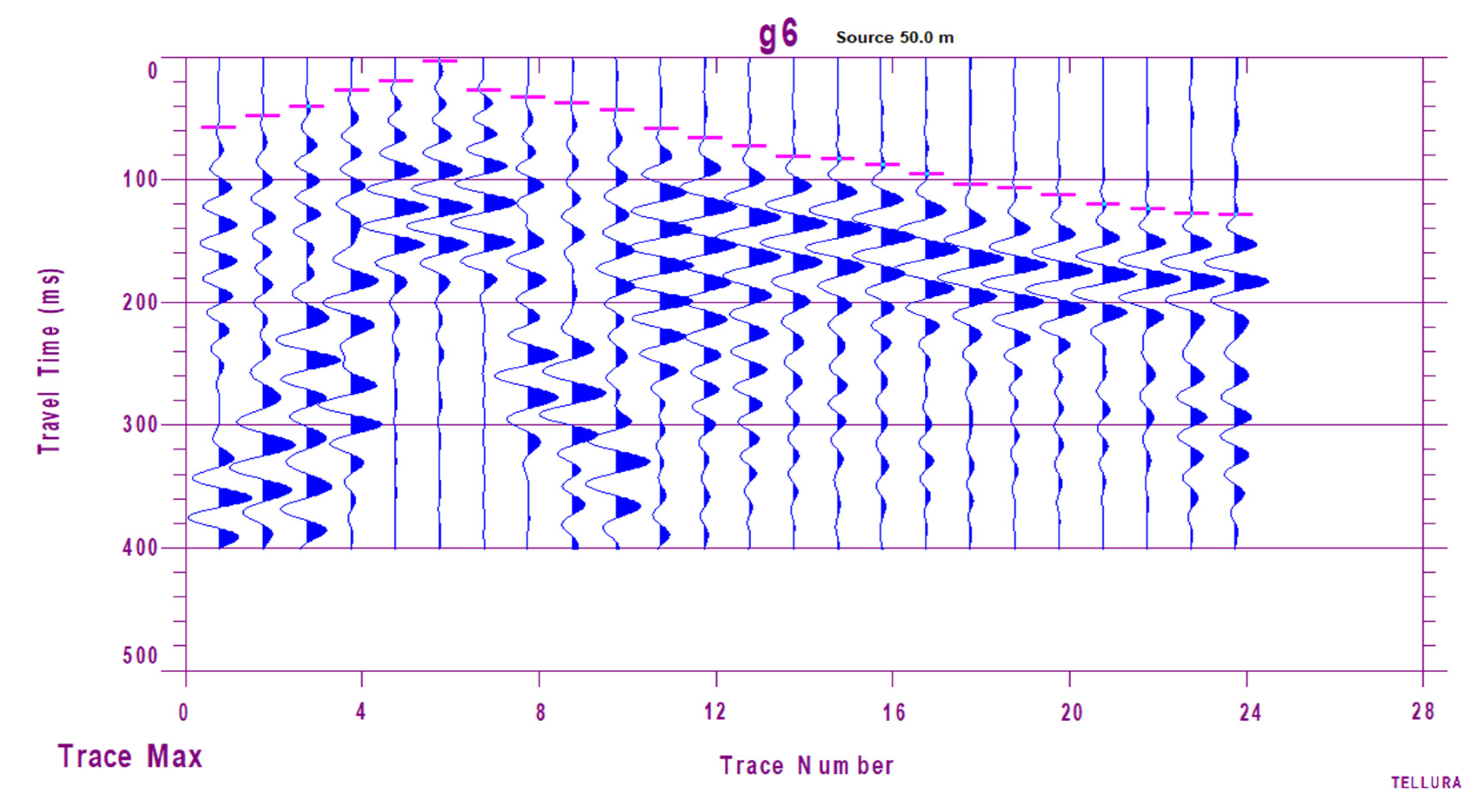
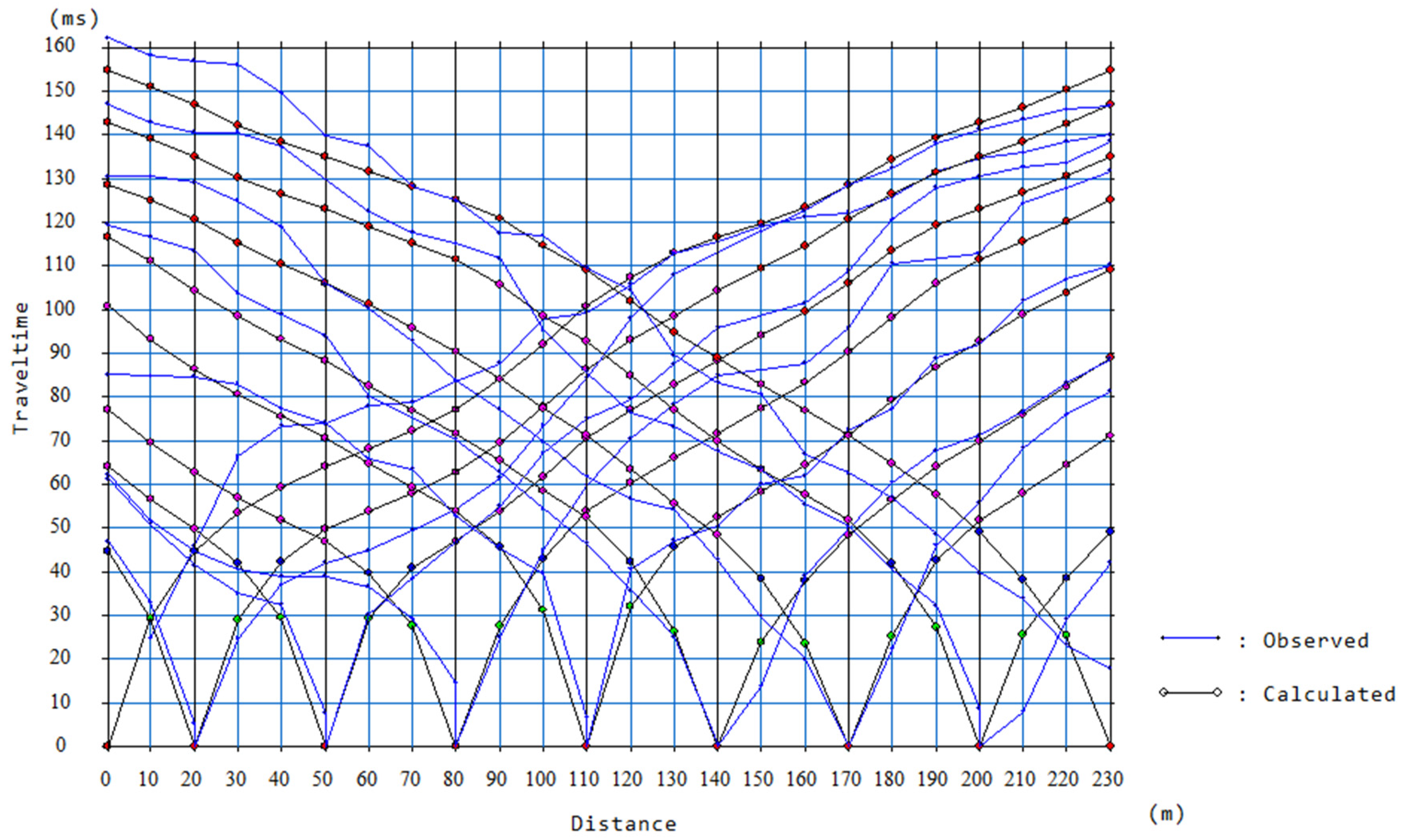
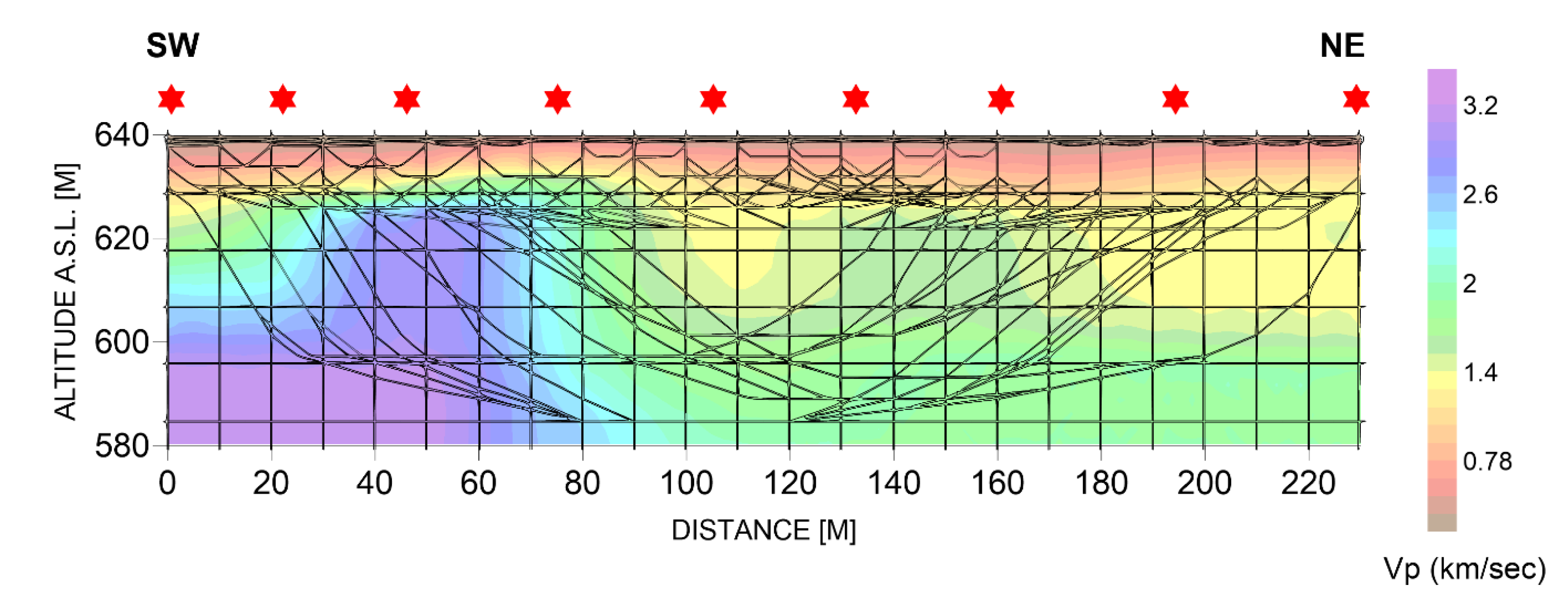
3.1. Seismic Refraction Data Acquisition and Processing
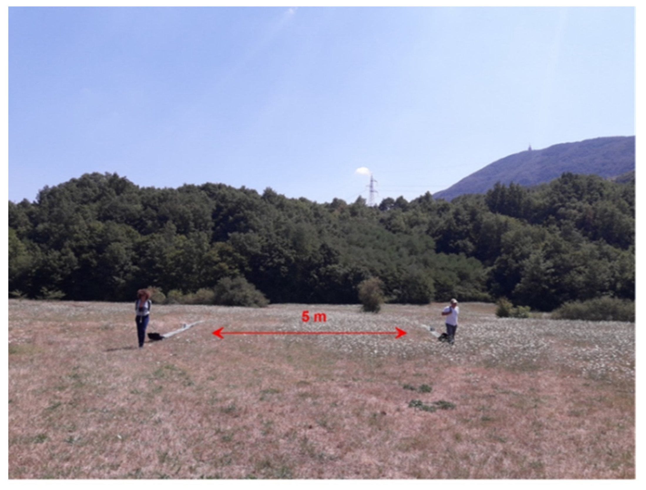
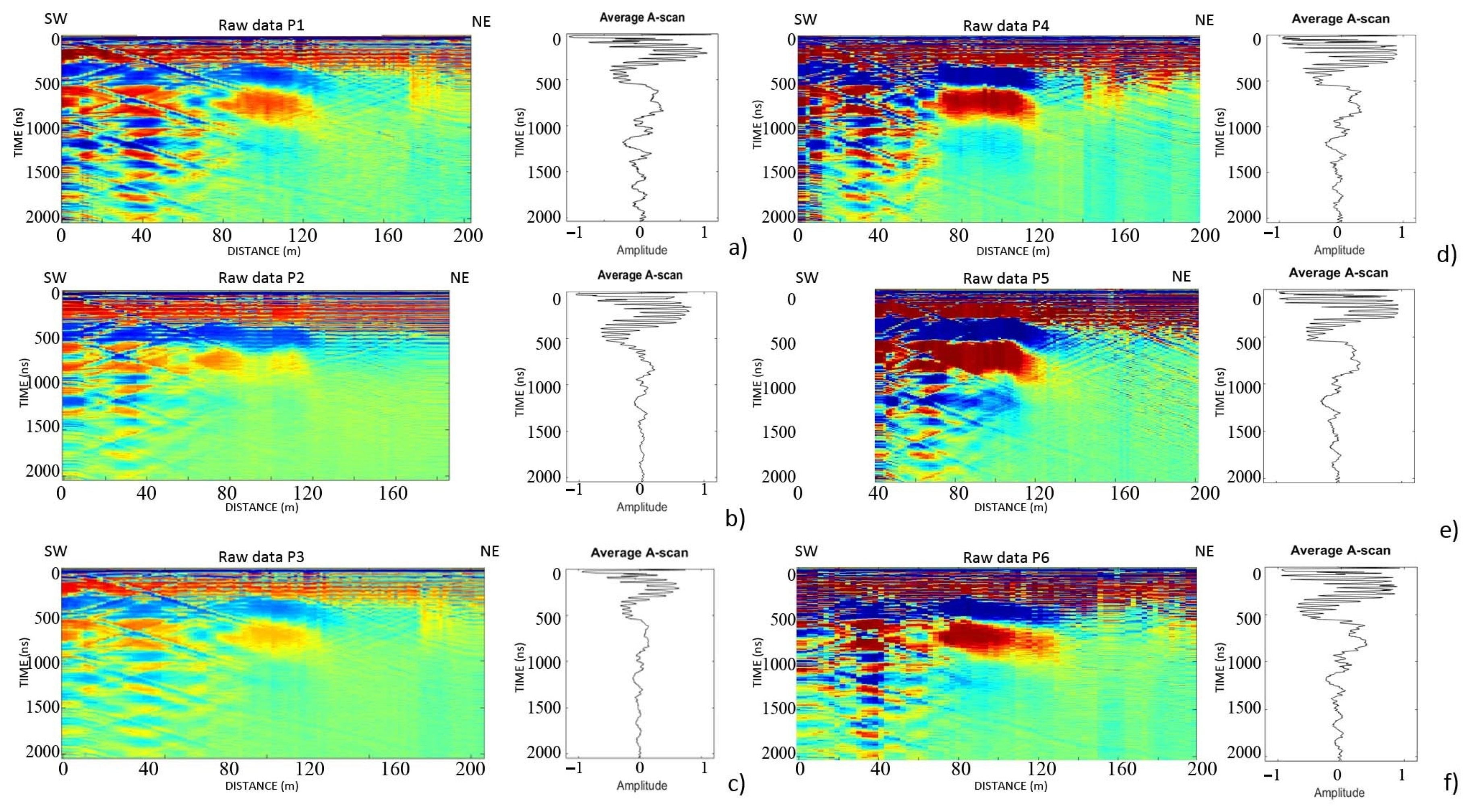
3.2. GPR Data Acquisition and Processing
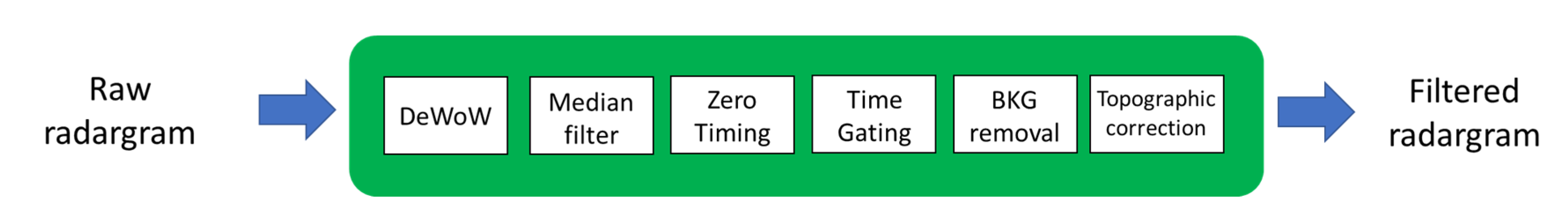
- (i)
- a high-power transmitter unit of 15 kV, 50 MW;
- (ii)
- a receiving unit to record broadband pulses with direct signal digitization, without stroboscopic conversion and 120 dB energy dynamic;
- (iii)
- two Wu–King antennas 6–15 m long without cable connection and with radio trigger placed on foils made of high-density polyethylene resistant to rubbing (Figure 7) that are resistively-loaded dipoles covered by a dielectric layer that avoids the dispersion of the transmitted signal;
- (iv)
- a controller connected to the receiver unit through a coaxial shielded multipolar cable.
- The DeWOW procedure subtracts at each collected waveforms its mean value along the time axis.
- The median filter, which allows removing noise from radargram and improving the results of later procedures [96].
- The zero timing defines the actual starting time, , of the observation time window.
- The time gating selects the portion of the observation time window where the target response occurs and allows eliminating the direct antenna coupling,, as well as the clutter signal, i.e., all the signals occurring outside the portion of the time windows of interest.
- Background (BKG) removal helps remove or mitigate the signal contributions due to antenna coupling, air–material interface, and (undesired) horizontal reflectors.
- Topographic correction inserts the real altitude of each acquired A-Scan and georeference the radargrams.
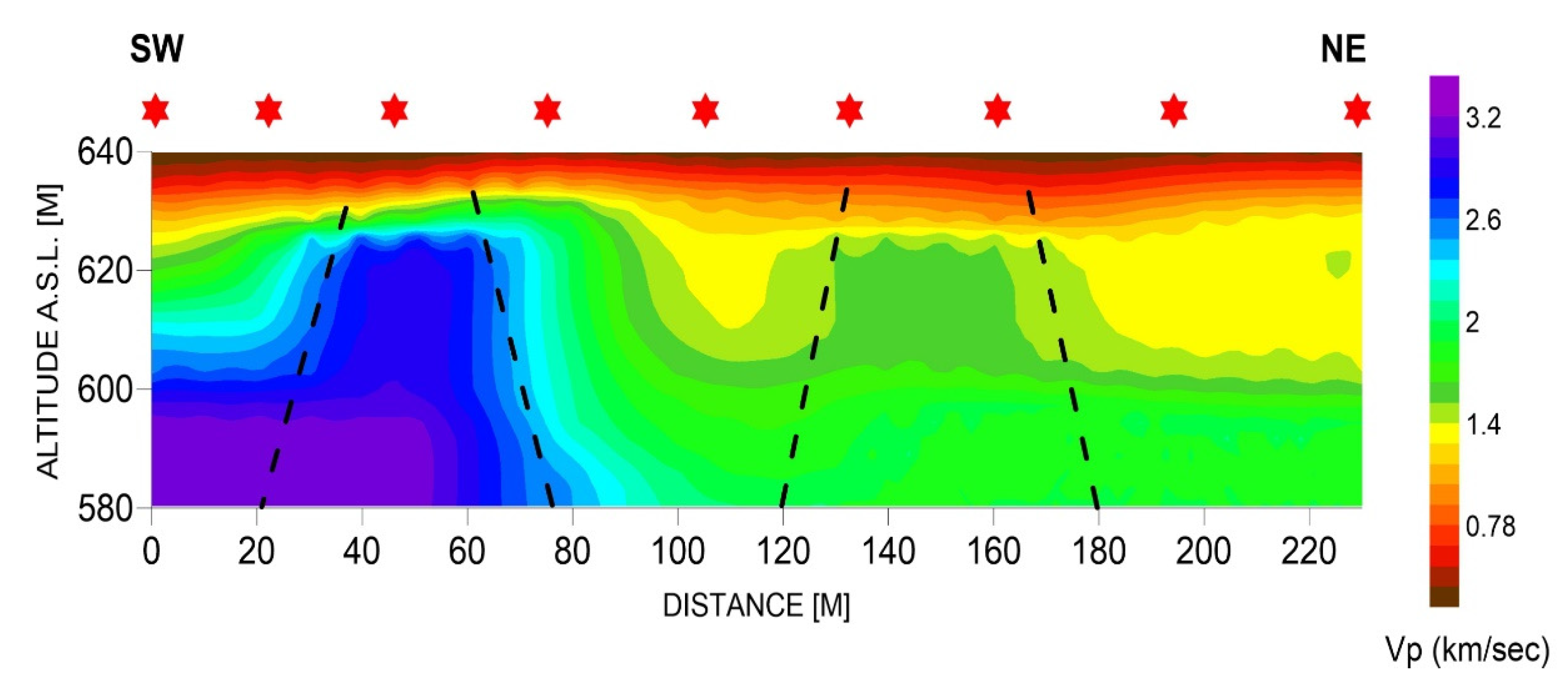
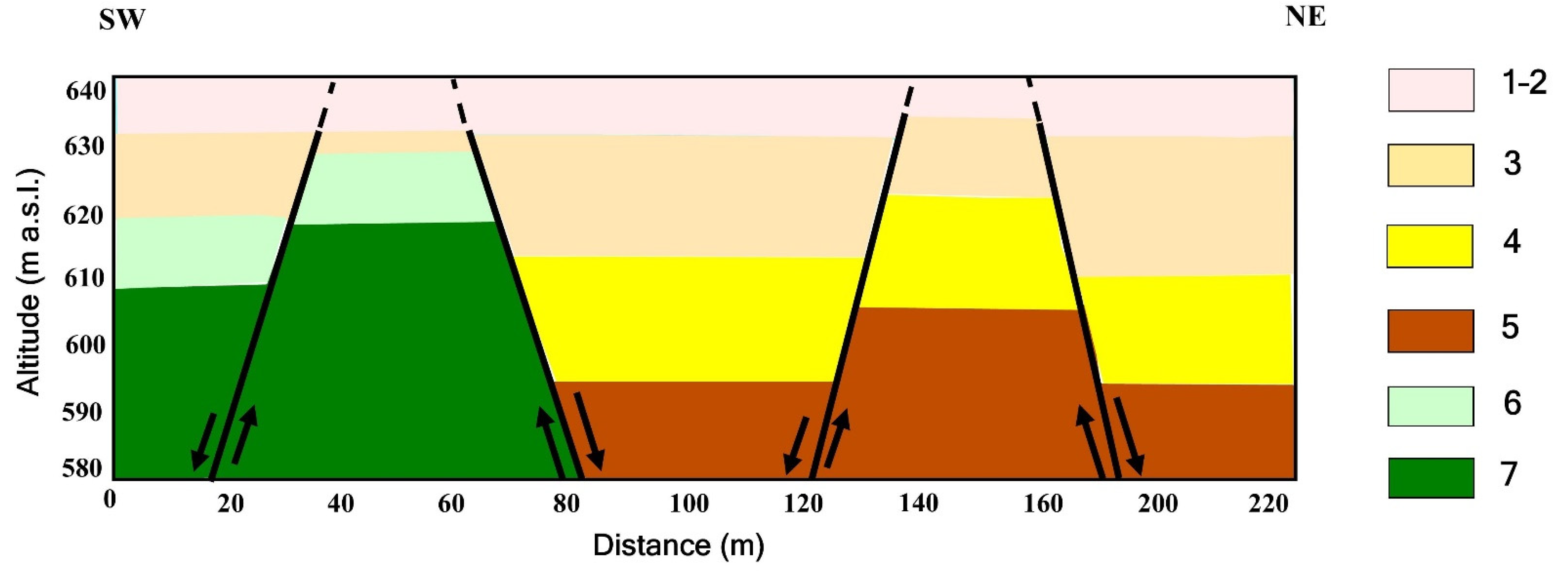
4. Results
5. Discussion
6. Conclusions
Author Contributions
Funding
Institutional Review Board Statement
Informed Consent Statement
Data Availability Statement
Acknowledgments
Conflicts of Interest
References
- Roberts, G.P.; Michetti, A.M. Spatial and temporal variations in growth rates along active normal fault systems: An example from The Lazio–Abruzzo Apennines, central Italy. J. Struct. Geol. 2004, 26, 339–376. [Google Scholar] [CrossRef]
- Jackson, J.; Leeder, M. Drainage systems and the development of normal faults: An example from Pleasant Valley, Nevada. J. Struct. Geol. 1994, 16, 1041–1059. [Google Scholar] [CrossRef]
- Bull, W.B. Tectonically Active Landscapes; Wiley Blackwell: Hoboken, NJ, USA, 2009; 320p, ISBN 978-1-4051-9012-1. [Google Scholar]
- Burbank, D.W.; Anderson, R.S. Tectonic Geomorphology, 2nd ed.; Wiley Blackwell: Hoboken, NJ, USA, 2011; p. 460. ISBN 978-1-444-33887-4. [Google Scholar]
- Ascione, A.; Nardò, S.; Mazzoli, S. The MS 6.9, 1980 Irpinia Earthquake from the Basement to the Surface: A Review of Tectonic Geomorphology and Geophysical Constraints, and New Data on Post-seismic Deformation. Geosciences 2020, 10, 493. [Google Scholar] [CrossRef]
- Galli, P. Roman to Middle Age Earthquakes Sourced by the 1980 Irpinia Fault: Historical, Archaeoseismological, and Paleoseismological Hints. Geosciences 2020, 10, 286. [Google Scholar] [CrossRef]
- Bello, S.; De Nardis, R.; Scarpa, R.; Brozzetti, F.; Cirillo, D.; Ferrarini, F.; Di Lieto, B.; Arrowsmith, R.; Lavecchia, G. Fault pattern and seismotectonic style of the Campania–Lucania 1980 earthquake (Mw 6.9, Southern Italy): New multidisciplinary constraints. Front. Earth Sci. 2021, 8, 652. [Google Scholar] [CrossRef]
- Aiello, G.; Ascione, A.; Barra, D.; Munno, R.; Petrosino, P.; Ermolli, E.R.; Villani, F. Evolution of the late Quaternary San Gregorio Magno tectono-karstic basin (southern Italy) inferred from geomorphological, tephrostratigraphical and palaeoecological analyses: Tectonic implications. J. Quat. Sci. 2007, 22, 233–245. [Google Scholar] [CrossRef]
- Galli, P.; Peronace, E. New paleoseismic data from the Irpinia Fault. A different seismogenic perspective for southern Apennines (Italy). Earth Sci. Rev. 2014, 136, 175–20110. [Google Scholar] [CrossRef]
- Improta, L.; Ferranti, L.; De Martini, P.M.; Piscitelli, S.; Bruno, P.P.; Burrato, P.; Civico, R.; Giocoli, A.; Iorio, M.; D’Addezio, G.; et al. Detecting young, slow-slipping active faults by geologic and multidisciplinary high-resolution geophysical investigations: A case study from the Apennine seismic belt, Italy. J. Geophys. Res. 2010, 115, B11307. [Google Scholar] [CrossRef] [Green Version]
- Everett, M.E. Near-Surface Applied Geophysics; Cambridge University Press: Cambridge, UK, 2013; 403p, ISBN 9781107018778. [Google Scholar]
- Villani, F.; Pucci, S.; Civico, R.; De Martini, P.M.; Nicolosi, I.; D’Ajello Caracciolo, F.; Carluccio, R.; Di Giulio, G.; Vassallo, M.; Smedile, A.; et al. Imaging the structural style of an active normal fault through multi-disciplinary geophysical investigation: A case study from the Mw 6.1, 2009 L’Aquila earthquake region (central Italy). Geophys. J. Int. 2015, 200, 1676–1691. [Google Scholar] [CrossRef] [Green Version]
- Luiso, P.; Paoletti, V.; Nappi, R.; Gaudiosi, G.; Cella, F.; Fedi, M. Testing the value of a multi/scale gravimetric analysis in characterizing active fault geometry at hypocentral depths: The 2016/2017 central Italy seismic sequence. Ann. Geophys. 2018, 61, DA558. [Google Scholar] [CrossRef]
- Luiso, P.; Paoletti, V.; Nappi, R.; La Manna, M.; Cella, F.; Gaudiosi, G.; Fedi, M.; Iorio, M. A multidisciplinary approach to characterize the geometry of active faults: The example of Mt. Massico, Southern Italy. Geophys. J. Int. 2018, 213, 1673–1681. [Google Scholar] [CrossRef]
- Galli, G.; Giaccio, B.; Messina, P.; Peronace, E.; Amato, V.; Naso, G.; Nomade, S.; Pereira, A.; Piscitelli, S.; Bellanova, J.; et al. Middle to Late Pleistocene activity of the northern Matese Fault System (southern Apennines, Italy). Tectonophysics 2017, 699, 61–81. [Google Scholar] [CrossRef]
- Ferrarini, F.; Boncio, P.; De Nardis, R.; Pappone, G.; Cesarano, M.; Aucelli, P.P.C.; Lavecchia, G. Segmentation pattern and structural complexities in seismogenic extensional setting: The north Matese Fault System (central Italy). J. Struct. Geol. 2017, 95, 93–112. [Google Scholar] [CrossRef]
- Meletti, C.; Patacca, E.; Scandone, P.; Figliuolo, B. Il terremoto del 1456 e la sua interpretazione nel quadro sismotettonico dell’Appennino meridionale. In Il Terremoto del 1456; Figliuolo, B., Ed.; Osservatorio Vesuviano e Istituto Italiano di Studi Filosofici, Storia e Scienze della Terra: Napoli, Italy, 1988; Volume 1, pp. 71–108. [Google Scholar]
- Locati, M.; Camassi, R.; Rovida, A.; Ercolani, E.; Bernardini, F.; Castelli, V.; Caracciolo, C.H.; Tertulliani, A.; Rossi, A.; Azzaro, R.; et al. DBMI15, the 2015 Version of the Italian Macroseismic Database; Istituto Nazionale di Geofisica e Vulcanologia: Rome, Italy, 2016. [Google Scholar] [CrossRef]
- Serva, L. The earthquake of 5 June, 1688 in Campania. In Atlas of Isoseismal Maps of Italian Earthquakes; Postpischl, D., Ed.; CNR-PFG: Rome, Italy, 1985; Volume 114, pp. 44–47. [Google Scholar]
- Esposito, E.; Luongo, G.; Marturano, A.; Porfido, S. Il terremoto di S. Anna del 26 Luglio 1805. Mem. Soc. Geol. Ital. 1987, 37, 171–191. [Google Scholar]
- Porfido, S.; Esposito, E.; Vittori, E.; Tranfaglia, G.; Michetti, A.M.; Blumetti, M.; Ferreli, L.; Guerreri, L.; Serva, L. Areal distribution of ground effect induced by strong earthquakes in the southern Apennines (Italy). Surv. Geophys. 2002, 23, 529–562. [Google Scholar] [CrossRef]
- Porfido, S.; Esposito, E.; Vittori, E.; Tranfaglia, G.; Guarrieri, L.; Pece, R. Seismically induced ground effects of the 1805, 1930 and 1980 earthquakes in the Southern Apennines (Italy). Boll. Soc. Geol. Ital. J. Geosci. 2007, 126, 333–346. [Google Scholar]
- DISS Working Group. Database of Individual Seismogenic Sources (DISS), Version 3.2.1; A Compilation of Potential Sources for Earthquakes Larger than M 5.5 in Italy and Surrounding Areas; Istituto Nazionale di Geofisica e Vulcanologia: Rome, Italy, 2018; Available online: http://diss.rm.ingv.it/diss/ (accessed on 1 February 2021). [CrossRef]
- Rovida, A.; Locati, M.; Camassi, R.; Lolli, B.; Gasperini, P. CPTI15, the 2015 Version of the Parametric Catalogue of Italian Earthquakes; Istituto Nazionale di Geofisica e Vulcanologia: Rome, Italy, 2016; 33p. [Google Scholar] [CrossRef]
- Michetti, A.M.; Blumetti, A.M.; Esposito, E.; Ferreli, L.; Guerrieri, L.; Porfido, S.; Serva, L.; Vittori, E. Earthquake ground effects and seismic hazard assessment in Italy examples from the Matese and Irpinia areas, Southern Apennines. Active Fault Research for the New Millennium. In Proceedings of the Hokudan Symposium and School on Active Faulting, Hokudan Town, Japan, 17–26 January 2000; pp. 279–284. [Google Scholar]
- Serva, L.; Esposito, E.; Guerrieri, L.; Porfido, S.; Vittori, E.; Comerci, V. Environmental effects from five historical earthquakes in Southern Apennines (Italy) and macroseismic intensity assessment. Contribution to INQUA EEE Scale Project. Quat. Intern. 2007, 173, 30–44. [Google Scholar] [CrossRef]
- Blumetti, A.M.; Caciagli, M.; Di Bucci, D.; Guerrieri, L.; Michetti, A.M.; Naso, G. Evidenze di fagliazione superficiale olocenica nel bacino di Bojano (Molise). In Proceedings of the 19° Meeting GNGTS, Rome, Italy, 7–9 November 2000; pp. 12–15. [Google Scholar]
- Westaway, R. Quaternary uplift of Southern Italy. J. Geophys. Res. 1993, 98, 21741–21772. [Google Scholar] [CrossRef]
- Cinque, A.; Patacca, E.; Scandone, P.; Tozzi, M. Quaternary kinematic evolution of the Southern Apennines. Relationship between surface geological features and deep lithospheric structures. Ann. Geof. 1993, 36, 249–260. [Google Scholar]
- Esposito, A.; Galvani, A.; Sepe, V.; Atzori, S.; Brandi, G.; Cubellis, E.; De Martino, P.; Dolce, M.; Massuccia, A.; Obrizzo, F.; et al. Concurrent deformation processes in the Matese massif area (Central-Southern Apennines, Italy). Tectonophysics 2020, 774, 228234. [Google Scholar] [CrossRef]
- Carafa, M.M.C.; Galvani, A.; Di Naccio, D.; Kastelic, V.; Di Lorenzo, C.; Miccolis, S.; Sepe, V.; Pietrantonio, G.; Gizzi, C.; Massucci, A.; et al. Partitioning the Ongoing Extension of the Central Apennines (Italy): Fault Slip Rates and Bulk Deformation Rates from Geodetic and Stress Data. J. Geophys. Res. Solid Earth 2020, 125, e2019JB018956. [Google Scholar] [CrossRef]
- Ferranti, L.; Palano, M.; Cannavò, F.; Mazzella, M.E.; Oldow, J.S.; Gueguen, E.; Mattia, M.; Monaco, C. Rates of geodetic deformation across active faults in southern Italy. Tectonophysics 2014, 621, 101–122. [Google Scholar] [CrossRef]
- Sgambato, C.; Faure Walker, J.; Mildon, Z.; Roberts, G.P. Fault/shear-zone system geometry and Coulomb pre-stress heterogeneity provides insights into stress-loading variability for earthquake faults. Sci. Rep. 2020, 10, 12724. [Google Scholar] [CrossRef] [PubMed]
- Giraudi, C.; Frezzotti, M. Paleoseismicity in the Gran Sasso Massif (Abruzzo, central Italy). Quat. Int. 1995, 25, 81–93. [Google Scholar] [CrossRef]
- Benedetti, L.; Manighetti, I.; Gaudemer, Y.; Finkel, R.; Malavieille, J.; Pou, K.; Arnold, M.; Aumaître, G.; Bourlès, D.; Keddadouche, K. Earthquake synchrony and clustering on Fucino faults (Central Italy) as revealed from in situ 36 Cl exposure dating. J. Geophys. Res. Solid Earth 2013, 118, 4948–4974. [Google Scholar] [CrossRef]
- Corrado, S.; Di Bucci, D.; Leschiutta, I.; Naso, G.; Trigari, A. La tettonica quaternaria della piana di Isernia nell’evoluzione strutturale del settore molisano. Il Quaternario 1997, 10, 609–614. [Google Scholar]
- Di Bucci, D.; Naso, G.; Corrado, S.; Villa, I.M. Growth, interaction and seismogenetic potential of coupled active normal faults (Isernia Basin, central-southern Italy). Terra Nova 2005, 17, 44–55. [Google Scholar] [CrossRef]
- Galli, P.; Galadini, F. Disruptive earthquakes revealed by faulted archaeological relics in Samnium (Molise, southern Italy). Geophys. Res. Lett. 2003, 30, 1266. [Google Scholar] [CrossRef]
- Galderisi, A.; Galli, P.; Mazzoli, S.; Peronace, E. Kinematic constraints of the active northern Matese Fault System (southern Italy). Boll. Geofis. Teor. Ed. Appl. 2017, 58, 285–302. [Google Scholar] [CrossRef]
- Ithaca Working Group. ITHACA (ITaly HAzard from CApable Faulting), A Database of Active Capable Faults of the Italian Territory. Version December 2019. ISPRA Geological Survey of Italy. Web Portal. Available online: http://sgi2.isprambiente.it/ithacaweb/Mappatura.aspx (accessed on 1 February 2021).
- De Corso, S.; Scrocca, D.; Tozzi, M. Geologia dell’anticlinale del Matese e implicazioni per la tettonica dell’Appennino molisano. Boll. Soc. Geol. Ital. 1998, 117, 419–441. [Google Scholar]
- Paolino, A.; Cogo, F. Da Pectoranum a Pettoranello di Molise; CEP Eds.: Monteroduni, Italy, 1990; pp. 1–95. [Google Scholar]
- GEMINA. Il bacino del Tammaro. In Ligniti e Torbe dell’Italia Continentale; Ilte: Torino, Italy, 1963; pp. 123–125. [Google Scholar]
- Vezzani, L.; Ghisetti, F.; Festa, A. Carta Geologica del Molise; scale 1:100,000, 1 sheet; S.EL.CA: Firenze, Italy, 2004. [Google Scholar]
- ISPRA. Note Illustrative della Carta Geologica d’Italia alla Scala 1:50.000, 2014, Foglio 405 “Campobasso”; Servizio Geologico Nazionale: Roma, Italy, 2014. [Google Scholar]
- Bernabini, M.; Eva, C.; Nicolich, R.; Baranello, S.; Cercato, M.; De Ferrari, R.; Ferretti, G.; Pellegrino, P.; Scapillati, N. Microzonazione sismica del comune di Bojano (CB). In Proceedings of the 28° GNGTS Convegno, Trieste, Italy, 16–19 November 2009; pp. 262–265. [Google Scholar]
- Amato, V.; Aucelli, P.P.C.; Cesarano, M.; Jicha, B.; Lebreton, V.; Orain, R.; Pappone, G.; Petrosino, P.; Russo Ermolli, E. Quaternary evolution of the largest intermontane basin of the Molise Apennine (central-southern Italy). Rend. Lincei 2014, 25, 197–216. [Google Scholar] [CrossRef]
- Amato, V.; Aucelli, P.P.C.; Cesarano, M.; Cifelli, F.; Leone, N.; Mattei, M.; Russo Ermolli, E.; Petrosino, P.; Rosskopf, C.M. The infill timing of a quaternary intermontane basin: New chrono-stratigraphic and palaeoenvironmental data by a 900 m deep borehole from Campochiaro (central-southern Apennine, Italy). In Proceedings of the Geophysical Research Abstracts, EGU General Assembly, Wien, Austria, 17–22 April 2016. [Google Scholar]
- Caciagli, M. Analisi della Tettonica Attiva Lungo la Struttura del M. Patalecchia Tra i Bacini d’Isernia e Bojano. Tesi di Laurea in Science Geologiche; La Sapienza: Roma, Italy, 1997; p. 112. (In Italian) [Google Scholar]
- Galli, P.; Galadini, F.; Capini, S. Analisi archeosismologiche nel santuario di Ercole di Campochiaro (Matese). Evidenze di un terremoto distruttivo sconosciuto ed implicazioni sismotettoniche. Il Quat. Ital. J. Quat. Sci. 2002, 15, 151–163. [Google Scholar]
- Magri, G.; Molin, D. Il Terremoto del dicembre 1456 nell’Appennino Centromeridionale; Comitato Nazionale Energia Nucleare: Rome, Italy, 1984; p. 180. (In Italian) [Google Scholar]
- Fracassi, U.; Valensise, G. Unveiling the sources of the catastrophic 1456 multiple earthquake: Hints to an unexplored tectonic mechanism in southern Italy. Boll. Seism. Soc. Am. 2007, 97, 725–748. [Google Scholar] [CrossRef] [Green Version]
- Maramai, A.; Brizuela, B.; Graziani, L. The Euro-Mediterranean tsunami catalogue. Ann. Geophys. 2014, 57, 1–26. [Google Scholar] [CrossRef]
- Milano, G.; Di Giovambattista, R.; Alessio, G. Earthquake swarms in the Southern Apennines chain (Italy): The 1997 seismic sequence in the Sannio–Matese mountains. Tectonophysics 1999, 306, 57–78. [Google Scholar] [CrossRef]
- Chiarabba, C.; De Gori, P.; Mele, F.M. Recent seismicity of Italy: Active tectonics of the central Mediterranean region and seismicity rate changes after the Mw 6.3 L’Aquila earthquake. Tectonophysics 2015, 638, 82–93. [Google Scholar] [CrossRef]
- Branno, A.; Esposito, E.; Luongo, G.; Marturano, A.; Porfido, S.; Rinaldis, V. The largest earthquakes of the Appennines, Southern Italy. In Proceedings of the International Symposium on Engineering Geology Problems in Seismic Areas, IAEG-AIGI, Bari, Italy, 13–14 April 1986; Volume 4, pp. 3–14. [Google Scholar]
- Alessio, G.; Godano, C.; Gorini, A. A low magnitude seismic sequence near Isernia (Molise, central Italy) in January 1986. Pure Appl. Geophys. 1990, 134, 243–260. [Google Scholar] [CrossRef]
- Vilardo, G.; Nappi, R.; Petti, P.; Ventura, G. Fault geometries from the space distribution of the 1990–1997 Sannio–Benevento earthquakes: Inferences on the active deformation in Southern Apennines. Tectonophysics 2003, 363, 259–271. [Google Scholar] [CrossRef]
- Milano, G.; Di Giovanbattista, R.; Ventura, G. The 2001 seismic activity near Isernia (Italy): Implications for the seismictectonics of the Central-Southern Appennines. Tecnophysics 2005, 401, 167–178. [Google Scholar] [CrossRef]
- ISIDe Working Group INGV. Italian Seismological Instrumental and Parametric Database; INGV: Roma, Italy, 2015. Available online: http://iside.rm.ingv.it/iside/standard/index.jsp (accessed on 1 February 2021).
- Fortini, P. Della cause de’ terremoti e loro effetti. Danni di quelli sofferti dalla città di Isernia fino a quello de’ 26 luglio 1805; Sardelli, T., Ed.; Marinelli Editore: Isernia, Italy, 1984; p. 65. [Google Scholar]
- Iadone, P. Relazione dettagliata di tutto ciò che ha rapport all’accaduto per causa del tremuoto della sera de’ 26 luglio corrente anno 1805, in questa città di Cajazzo, e sua diocesi, conformemente all’istruzione ricevute per tal’ oggetto con dispaccio di 5 agosto. Colloquio sulle scienze della terra in onore di Nicola Covelli 1805. Ass. Storica del Caratino 1805, 8, 33–66. [Google Scholar]
- Poli, G.S. Memoria sul Tremuoto de’ 26 Luglio del Corrente Anno 1805; Ed. Orsino: Napoli, Italy, 1806; p. 225. [Google Scholar]
- Pepe, G. Ragguaglio Historico-Fisico del Tremuoto Accaduto nel Regno di Napoli la Sera de 26 Luglio 1805; Giacomo, S., Ed.; Domenico Sangiacomo: Napoli, Italy, 1806; p. 174. [Google Scholar]
- Capozzi, G. Memoria sul Tremuoto Avvenuto nel Contado di Molise nella Sera de 26 Luglio dell’Anno 1805; Independently Published: Benevento, Italy, 1834. [Google Scholar]
- Guerrieri, L.; Scarascia Mugnozza, G.; Vittori, E. Analisi stratigrafica e geomorfologica della conoide tardo-quaternaria di Campochiaro ed implicazioni per la conca di Bojano in Molise. Il Quaternario 1999, 12, 237–247. [Google Scholar]
- Michetti, A.M.; Esposito, E.; Guerrieri, L.; Porfido, S.; Serva, L.; Tatevossian, R.; Vittori, E.; Audemard, F.; Azuma, T.; Clague, J.; et al. Intensity Scale ESI 2007. Mem. Descr. Carta Geol. Ital. 2007, 74, 7–54. [Google Scholar]
- Serva, L.; Vittori, E.; Comerci, V.; Esposito, E.; Guerrieri, L.; Michetti, A.M.; Mohammadioun, B.; Porfido, S.; Tatevossian, R.E. Earthquake Hazard and the Environmental Seismic Intensity (ESI) Scale. Pure Appl. Geophys. 2016, 173, 1479–1515. [Google Scholar] [CrossRef]
- Cucci, L. Insights into the geometry and faulting style of the causative faults of the M6.7 1805 and M6.7 1930 earthquakes in the Southern Apennines (Italy) from coseismic hydrological changes. Tectonophysics 2019, 751, 192–211. [Google Scholar] [CrossRef]
- Cucci, L.; D’Addezio, G.; Valensise, G.; Burrato, P. Investigating seismogenic faults in Central and Southern Apennines (Italy): Modeling of fault-related landscape features. Ann. Geofis. 1996, 39, 603–618. [Google Scholar]
- Shebalin, N.V. Macroseismic data as information on source parameters of large earthquakes. Phys. Earth. Planet. Inter. 1972, 6, 316–323. [Google Scholar] [CrossRef]
- Esposito, E.; Luongo, G.; Petrazzuoli, S.M.; Porfido, S. Damage scenarious introduced by the major seismic events from XV to XIX century in Naples city with particular references to the seismic response. In Proceedings of the 10th World Conference on Earthquake Engeenering, Madrid, Spain, 19–24 July 1992; pp. 1075–1080. [Google Scholar]
- Esposito, E.; Pece, R.; Porfido, S.; Tranfaglia, G. Hydrological anomalies connected to earthquakes in Southern Apennines (Italy). Nat. Hazards Earth Syst. Sci. 2001, 1, 137–144. [Google Scholar] [CrossRef] [Green Version]
- Bruno, P.P.; Castiello, A.; Improta, L. Ultrashallow seismic imaging of the causative fault of the 1980, M6.9, southern Italy earthquake by pre-stack depth migration of dense wide-aperture data. Geophys. Res. Lett. 2010, 37, L19302. [Google Scholar] [CrossRef]
- Catapano, I.; Gennarelli, G.; Ludeno, G.; Soldovieri, F.; Persico, R. Ground-Penetrating Radar: Operation Principle and Data Processing. In Wiley Encyclopedia of Electrical and Electronics Engineering; Webster, J.G., Ed.; Wiley & Sons: Hoboken, NJ, USA, 2019; pp. 1–23. [Google Scholar] [CrossRef]
- Capozzoli, L.; De Martino, G.; Polemio, M.; Rizzo, E. Geophysical techniques for monitoring settlement phenomena occurring in reinforced concrete buildings. Surv. Geophys. 2020, 41, 575–604. [Google Scholar] [CrossRef]
- Rizzo, E.; Capozzoli, L.; De Martino, G.; Grimaldi, S. Urban Geophysical approach to characterize the subsoil of the main square in San Benedetto del Tronto town (Italy). J. Eng. Geol. 2019, 257, 105133. [Google Scholar] [CrossRef]
- Green, A.G.; Gross, R.; Holliger, K.; Horstmeyer, H.; Baldwin, J. Results of 3-D georadar surveying and trenching the San Andreas fault near its northern landwardlimit. Tectonophysics 2003, 368, 7–23. [Google Scholar] [CrossRef]
- Gross, R.; Green, A.G.; Horstmeyer, H.; Holliger, K.; Baldwin, J. 3-D georadar images of an active fault: Efficient data acquisition, processing and interpretation strategies. Subsurf. Sens. Technol. Appl. 2003, 4, 19–40. [Google Scholar] [CrossRef]
- Jewell, C.J.; Bristow, C.S. GPR studies in the Piano di Pezza area of the Ovindoli-Pezza Fault, Central Apennines, Italy: Extending paleoseismic trench investigations with high resolution GPR profiling. Near Surf. Geophys. 2006, 3, 65. [Google Scholar] [CrossRef]
- Vanneste, K.; Verbeeck, K.; Petermans, T. Pseudo-3D imaging of a low-slip-rate active normal fault using shallow geophysical methods: The Geleen fault in the Belgian Mass River valley. Geophysics 2008, 73, B1–B9. [Google Scholar] [CrossRef]
- Christie, M.; Tsoflias, G.P.; Stockli, D.F.; Black, R. Assessing fault displacement and off-fault deformation in an extensional tectonic setting using 3-D groundpenetrating radar imaging. J. Appl. Geophys. 2009, 68, 9–16. [Google Scholar] [CrossRef]
- Pauselli, C.; Federico, C.; Frigeri, A.; Orosei, R.; Barchi, M.R.; Basile, G. Ground penetrating radar investigations to study active faults in the Norcia Basin (Central Italy). J. Appl. Geophys. 2010, 72, 39–45. [Google Scholar] [CrossRef]
- McClymont, A.F.; Green, A.G.; Kaiser, A.; Horstmeyer, H.; Langridge, R. Shallow fault segmentation of the Alpine fault zone, New Zealand revealed from 2- and 3-D GPR surveying. J. Appl. Geophys. 2010, 70, 343–354. [Google Scholar] [CrossRef]
- Carpentier, S.F.A.; Green, A.G.; Langridge, R.; Boschetti, S.; Doetsch, J.; Abächerli, A.N.; Horstmeyer, H.; Finnemore, M. Flower structures and Riedel shears at a step over zone along the Alpine Fault (New Zealand) inferred from 2-D and 3-D GPR images. J. Geophys. Res. 2012, 117, B02406. [Google Scholar] [CrossRef]
- Ercoli, M.; Pauselli, C.; Frigeri, A.; Forte, E.; Federico, C. “Geophysical paleoseismology” through high resolution GPR data: A case of shallow faulting imaging in Central Italy. J. Appl. Geophys. 2013, 90, 27–40. [Google Scholar] [CrossRef]
- Ercoli, M.; Pauselli, C.; Frigeri, A.; Forte, E.; Federico, C. 3-D GPR data analysis for high-resolution imaging of shallow subsurface faults: The Mt Vettore case study (Central Apennines, Italy). Geophys. J. Int. 2014, 198, 609–621. [Google Scholar] [CrossRef] [Green Version]
- Kopeikin, V.V.; Kuznetsov, V.D.; Morozov, P.A.; Popov, A.V.; Berkut, A.I.; Merkulov, S.V.; Alexeev, V.A. Ground penetrating radar investigation of the supposed fall site of a fragment of the Chelabinsk meteorite in Lake Chebarkul’. Geochem. Int. 2013, 51, 575–582. [Google Scholar] [CrossRef]
- Buzin, V.; Edemsky, D.; Gudoshnikov, S.; Kopeikin, V.; Morozov, P.; Popov, A.; Prokopovich, I.; Skomarovsky, V.; Melnik, N.; Berkut, A.; et al. Search for Chelyabinsk Meteorite Fragments in Chebarkul Lake Bottom (GPR and Magnetic Data). J. Telecommun. Inf. Technol. 2017, 69–78. [Google Scholar] [CrossRef]
- Prokopovich, I.; Edemsky, A.D.; Popov, P.; Morozov, P.A. GPR Survey of Fortification Objects on Matua Island. In Proceedings of the 17th International Conference on Ground Penetrating Radar (GPR), Rapperswil, Switzerland, 18–21 June 2018; IEEE Xplore. pp. 1–4. [Google Scholar] [CrossRef]
- Rezaei, A.; Hassani, H.; Moarefvand, P.; Golmohammadi, A. Determination of unstable tectonic zones in C–North deposit, Sangan, NE Iran using GPR method: Importance of structural geology’. J. Min. Environ. 2019, 10, 177–195. [Google Scholar] [CrossRef]
- Daniels, D.J. Ground penetrating radar. In Encyclopedia of RF and Microwave Engineering; Wiley & Sons, Inc.: Hoboken, NJ, USA, 2005. [Google Scholar] [CrossRef]
- Kopeikin, V.V.; Morozov, P.A.; Edemskiy, F.D.; Edemskiy, D.E.; Pavloskii, B.R.; Sungurov, Y.A. Experience of GPR Application in Oil-and-Gas Industry. In Proceedings of the 14th International Conference on Ground Penetrating Radar (GPR), Shanghai, China, 4–8 June 2012. [Google Scholar] [CrossRef]
- Persico, R. Introduction to Ground Penetrating Radar: Inverse Scattering and Data Processing; Wiley-IEEE: Hoboken, NJ, USA, 2014; ISBN 978-1-118-30500-3. [Google Scholar]
- Ludeno, G.; Capozzoli, L.; Rizzo, E.; Soldovieri, F.; Catapano, I.A. Microwave Tomography Strategy for Underwater Imaging via Ground Penetrating Radar. Remote Sens. 2018, 10, 1410. [Google Scholar] [CrossRef] [Green Version]
- Oskooi, B.; Parnow, S.; Smirnov, M.; Varfinezhad, R.; Yari, M. Attenuation of random noise in GPR data by image processing. Arab. J. Geosci. 2018, 11, 677. [Google Scholar] [CrossRef]
- Slemmons, D.B. Geological effects of the Dixie Valley—Fairview Peak, Nevada, earthquakes of December 16, 1954. Bull. Seismol. Soc. Am. 1957, 47, 353–375. [Google Scholar]
- Caskey, S.J.; Wesnousky, S.G. Static stress changes and earthquake triggering during the 1954 Fairview Peak and Dixie Valley earthquakes, central Nevada. Bull. Seismol. Soc. Am. 1997, 87, 521–527. [Google Scholar]
- Zuo, J.; Wu, Z.H.; Ha, G.; Hu, M.; Zhou, C.; Gai, H. Spatial variation of nearly NS-trending normal faulting in the southern Yadong-Gulu rift, Tibet: New constraints from the Chongba Yumtso fault, Duoqing Co graben. J. Struct. Geol. 2021, 144, 104256. [Google Scholar] [CrossRef]
- Pantosti, D.; Schwartz, D.P.; Valensise, G. Paleoseismology along the 1980 surface rupture of the Irpinia fault: Implications for earthquake recurrence in the Southern Apennines, Italy. J. Geophys. Res. 1993, 98, 6561–6577. [Google Scholar] [CrossRef]


| Location | Type | Historical Description | Ref. | Note |
|---|---|---|---|---|
| Miranda S. Angelo in Grotte | Surface faulting/ground crack | “A very long fracture was surveyed from Miranda, Pesche up to S. Angelo in Grotte. Especially in the upper mountain from Miranda to S. Angelo in Grotte chasms were open for about a half palm.” | [61] | One Neapolitan palm = 26.3 cm |
| Matese Mt. Guardiaregia Morcone From Campobasso to Bussi Isernia (Mt. Patalecchia) Carpinone | Surface faulting/ground crack | “In the Matese and other mountains of the county have made considerable cracks. Very evident and deep fractures with offsets up to seven palms... you can also see horrible cracks of stones in the northern flank of Guardiareggia, and in the southern flank of Isernia. A third can be admired north of Carpinone…” | [63] | Offset of about 150 cm |
| Pesche Carpinone Guardia regia Matese Mt Salcito Trivento Montagano Morcone | Surface faulting/ground crack | “An opening wider than a Neapolitan palm, and more than two miles long was found throughout the back of the hill of Pesche…Carpinone also had in its surroundings two cracks, as still Guardia Regia, ... The surface of Mount Matese is all traced of considerable cracks... Equally considerable cracks were observed in the lands of Salcito, Trivento, Montagano, and Morcone...” | [64] | 1 mile = 1845.69 m |
| Morcone | Surface faulting/ground crack | “Horrible chasms opened over a length of about one-third of a mile, some of which had the ground overthrown at a height exceeding two palms, and of which the width was over three palms and comparable the depth. These fractures now can be seen from far away, because the grass along the crevasses is desiccated as it had been on fire. In one such crevasse I observed a pear tree, that, in that moment [of the earthquake], lost all its unripe fruits, threw many branches to the ground and, of the ones left, many are now desiccated. In the same place the soil was completely disturbed, as it had excavated by innumerable moles.” | [65] | 1 mile = 1845.69 m |
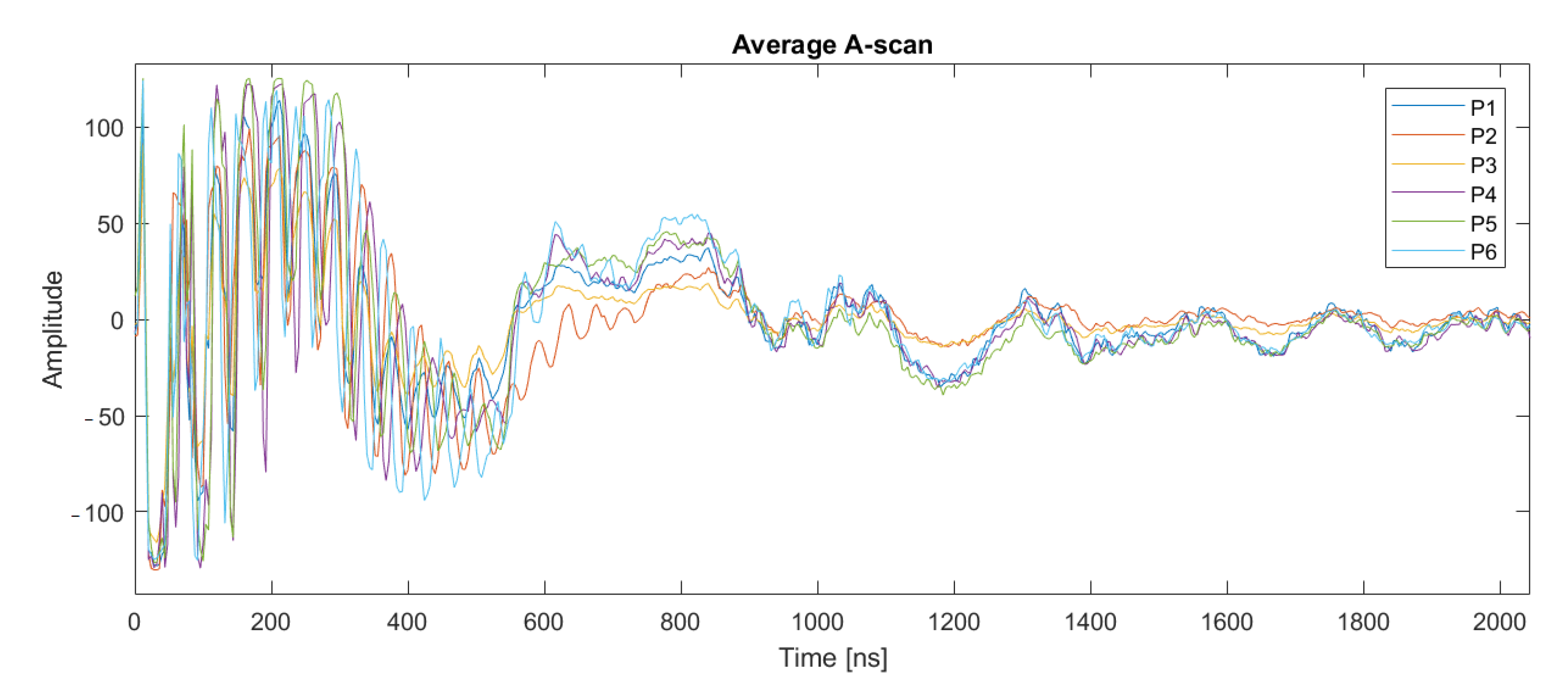
| ID Data | Length (m) | Spatial Step (m) | Frequency (MHz) | Easting Start (UTM-m) | Northing Start (UTM-m) | Easting End (UTM-m) | Northing End (UTM-m) |
|---|---|---|---|---|---|---|---|
| P1 | 203 | 2.5 | 15 | 440,755.19 | 4,601,386.77 | 440,890.79 | 4,601,538.72 |
| P2 | 185 | 2.5 | 15 | 440,801.55 | 4,601,373.14 | 440,951.19 | 4,601,479.89 |
| P3 | 206 | 2.4 | 15 | 440,880.19 | 4,601,312.10 | 441,033.00 | 4,601,446.72 |
| P4 | 199 | 2.3 | 15 | 440,988.88 | 4,601,231.02 | 441,142.06 | 4,601,359.67 |
| P5 | 160 | 1.6 | 15 | 441,078.61 | 4,601,207.34 | 441,202.22 | 4,601,319.15 |
| P6 | 198 | 3.3 | 25 | 441,138.12 | 4,601,115.96 | 441,290.82 | 4,601,233.27 |
Publisher’s Note: MDPI stays neutral with regard to jurisdictional claims in published maps and institutional affiliations. |
© 2021 by the authors. Licensee MDPI, Basel, Switzerland. This article is an open access article distributed under the terms and conditions of the Creative Commons Attribution (CC BY) license (https://creativecommons.org/licenses/by/4.0/).
Share and Cite
Nappi, R.; Paoletti, V.; D’Antonio, D.; Soldovieri, F.; Capozzoli, L.; Ludeno, G.; Porfido, S.; Michetti, A.M. Joint Interpretation of Geophysical Results and Geological Observations for Detecting Buried Active Faults: The Case of the “Il Lago” Plain (Pettoranello del Molise, Italy). Remote Sens. 2021, 13, 1555. https://0-doi-org.brum.beds.ac.uk/10.3390/rs13081555
Nappi R, Paoletti V, D’Antonio D, Soldovieri F, Capozzoli L, Ludeno G, Porfido S, Michetti AM. Joint Interpretation of Geophysical Results and Geological Observations for Detecting Buried Active Faults: The Case of the “Il Lago” Plain (Pettoranello del Molise, Italy). Remote Sensing. 2021; 13(8):1555. https://0-doi-org.brum.beds.ac.uk/10.3390/rs13081555
Chicago/Turabian StyleNappi, Rosa, Valeria Paoletti, Donato D’Antonio, Francesco Soldovieri, Luigi Capozzoli, Giovanni Ludeno, Sabina Porfido, and Alessandro Maria Michetti. 2021. "Joint Interpretation of Geophysical Results and Geological Observations for Detecting Buried Active Faults: The Case of the “Il Lago” Plain (Pettoranello del Molise, Italy)" Remote Sensing 13, no. 8: 1555. https://0-doi-org.brum.beds.ac.uk/10.3390/rs13081555