
Effect of Time of Day and Sky Conditions on Different Vegetation Indices Calculated from Active and Passive Sensors and Images Taken from UAV


 and
and
Abstract
:
1. Introduction
2. Materials and Methods
2.1. Experimental Site
2.2. Spectral Reflectance Measurements
2.3. Data Analysis
3. Results
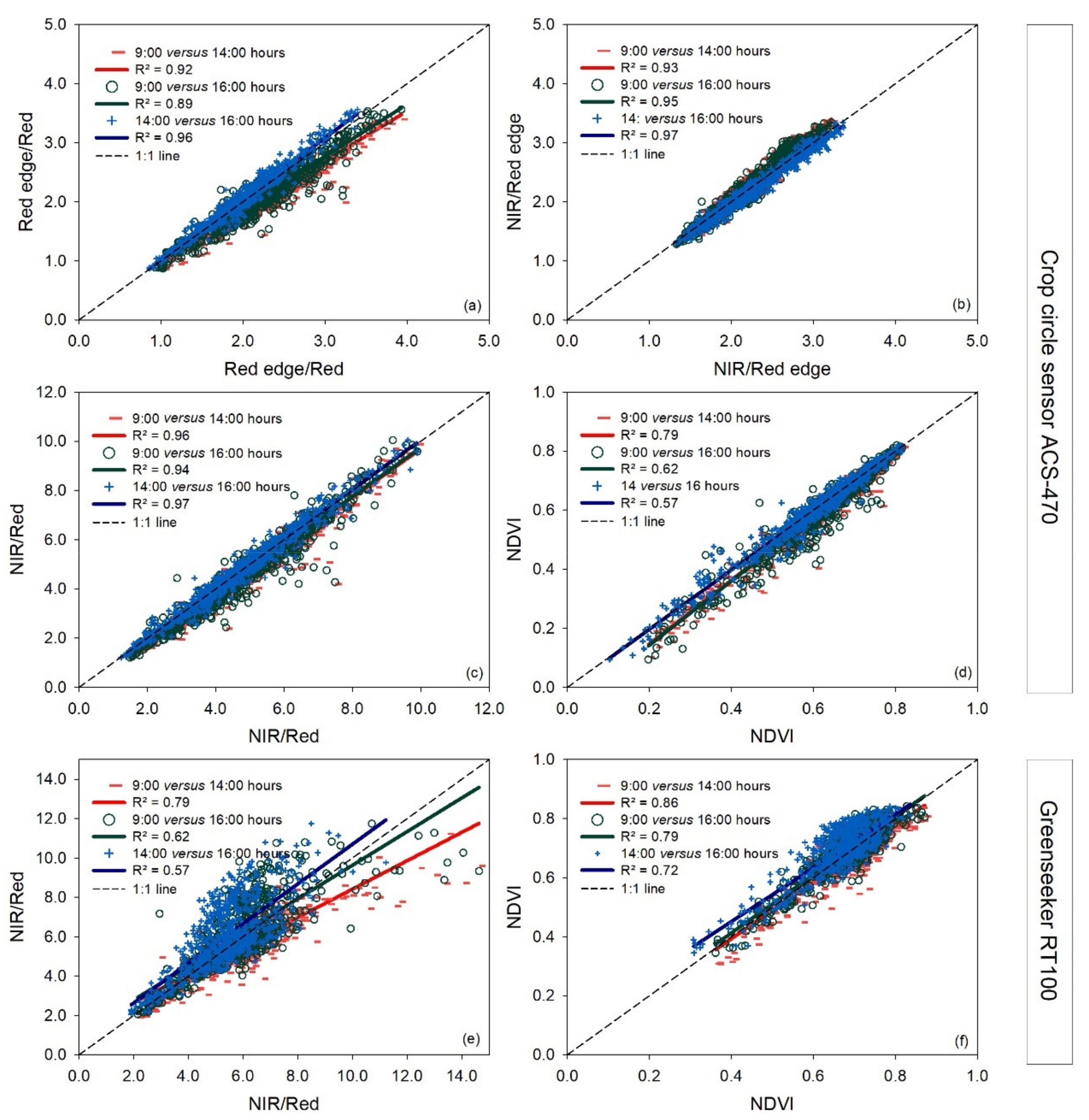
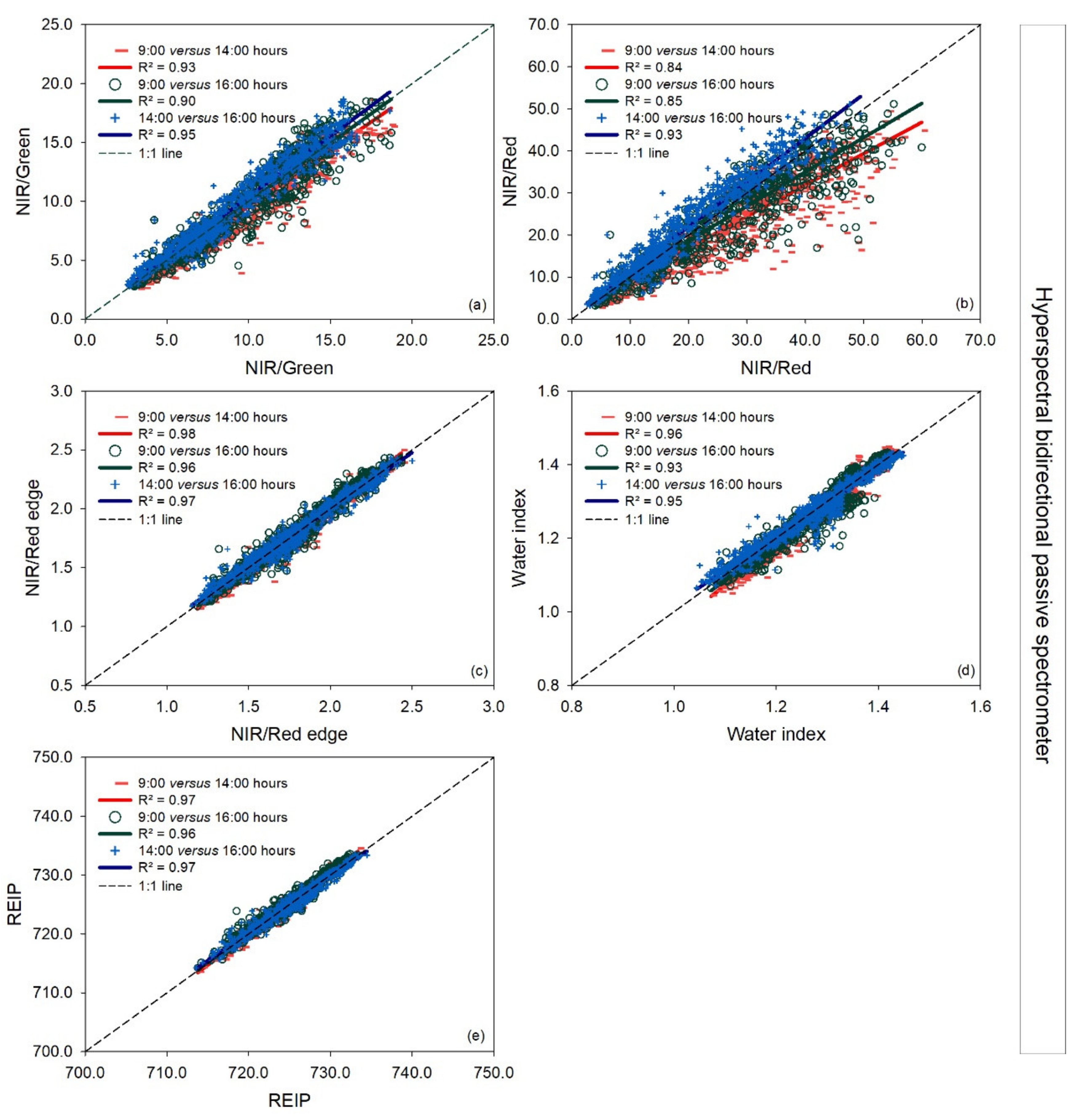
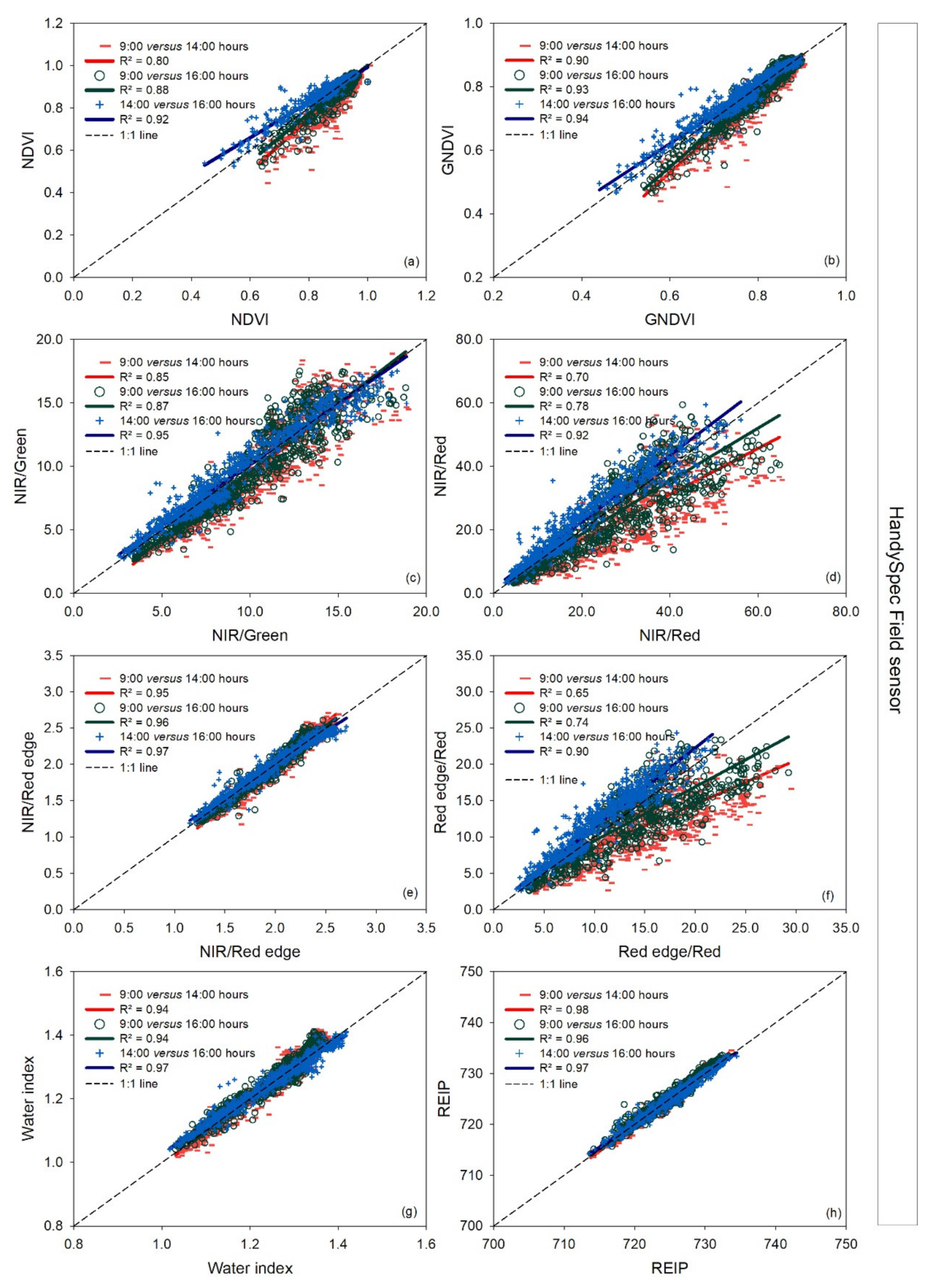
3.1. Evaluation of Time of Day Effects
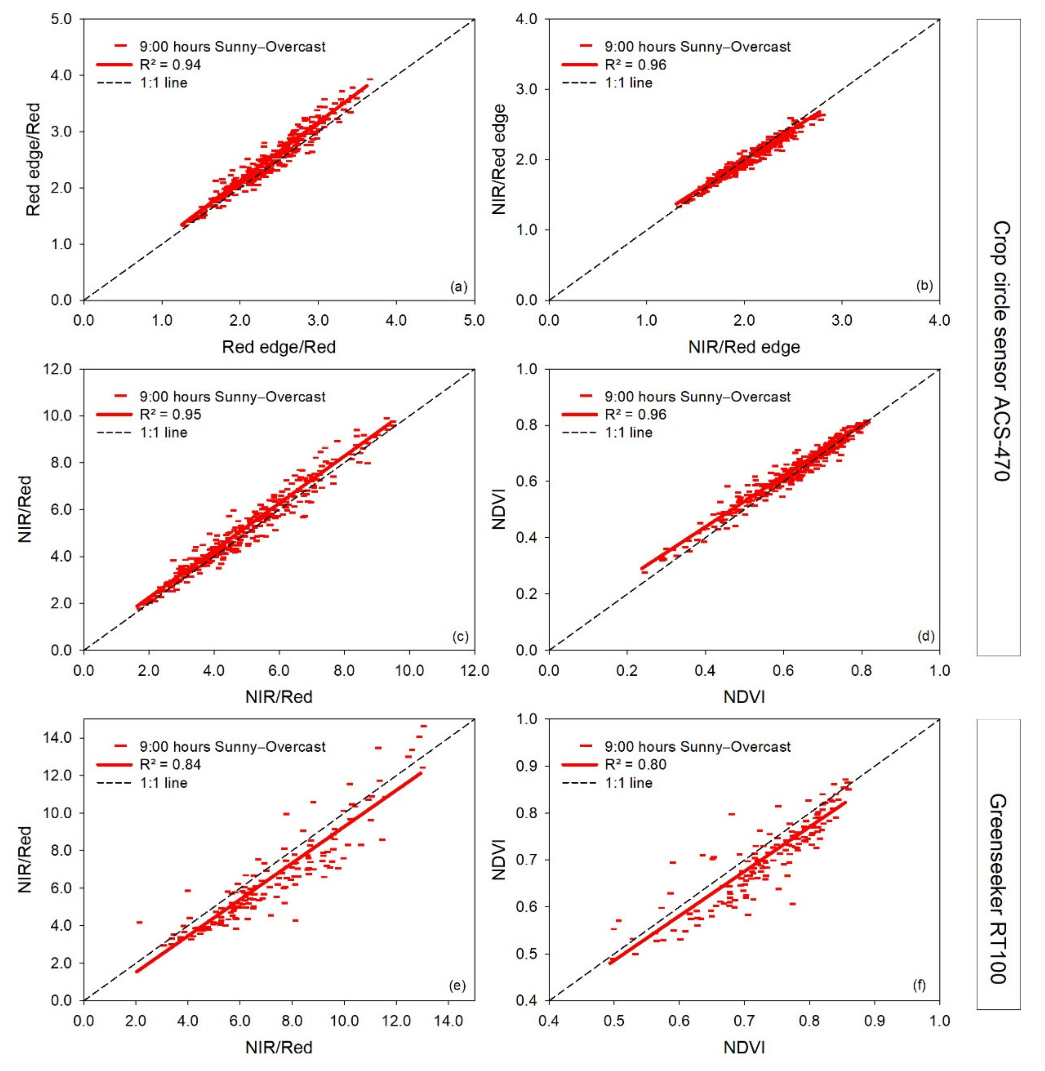
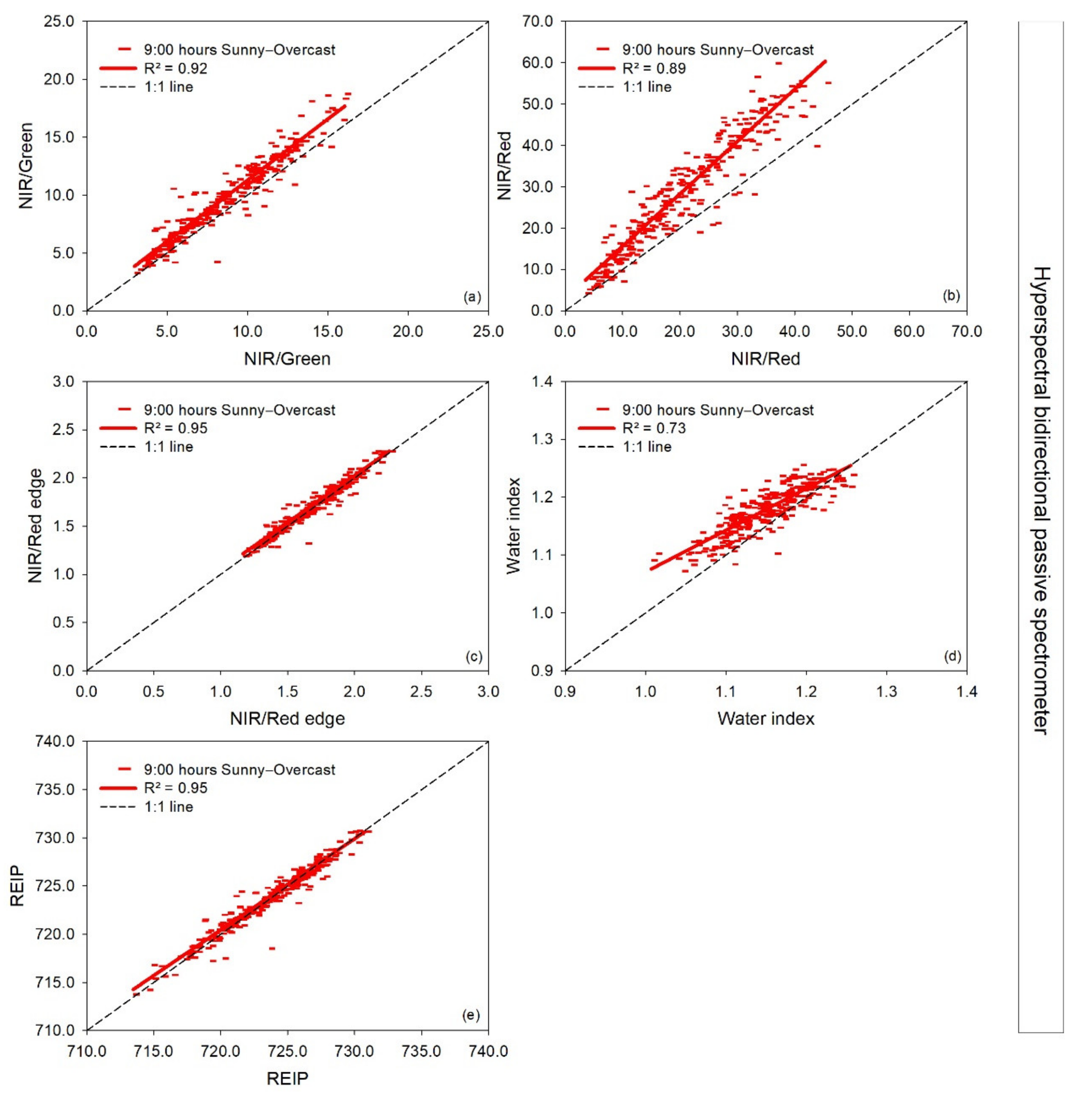
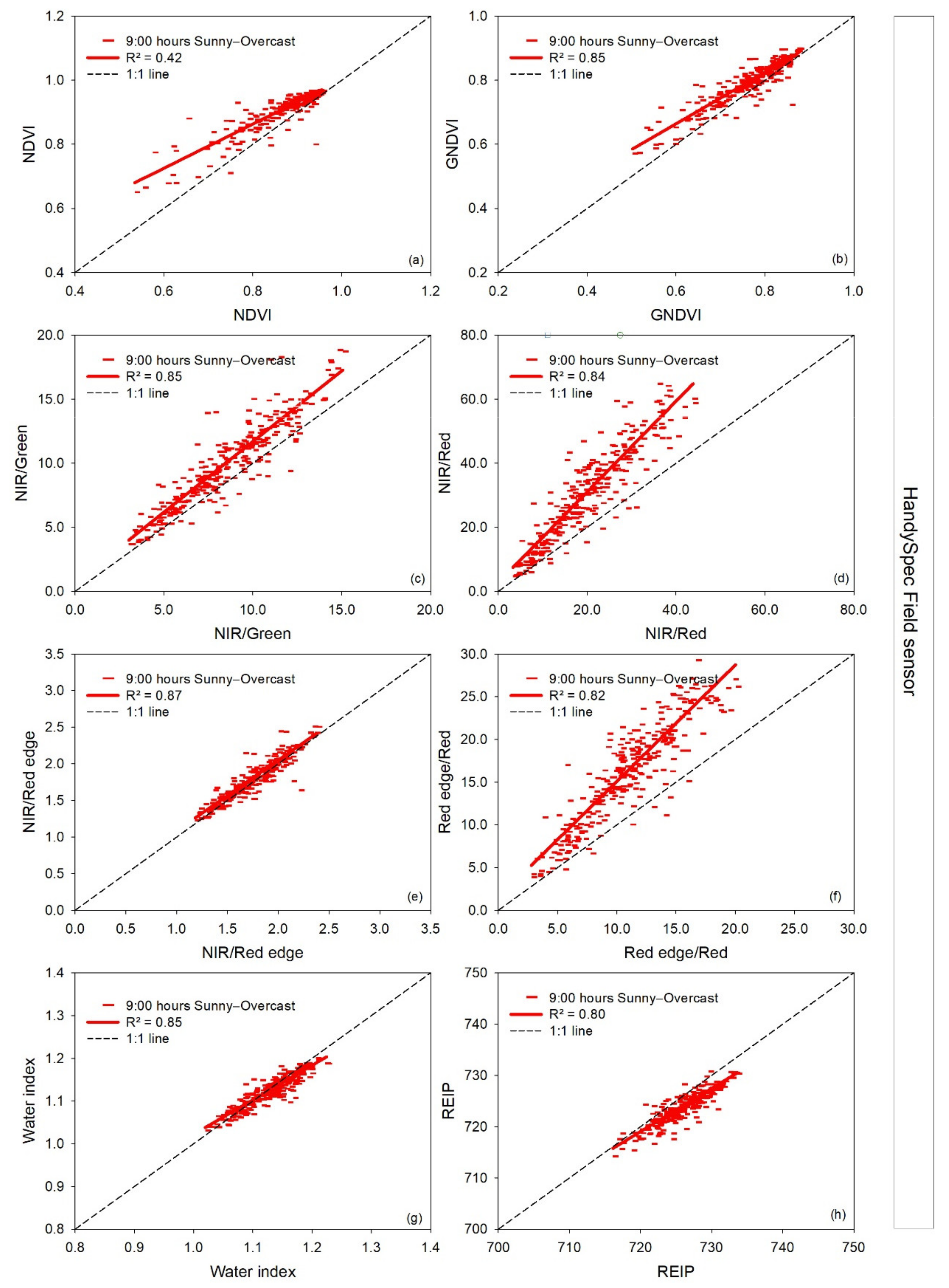
3.2. Evaluation of Sky Conditions Effects
4. Discussion
4.1. General Effects of Time of Day
4.2. Sensor Specific Performance Influenced by Time of Day
4.3. Evaluation of Sky Condition Effects
5. Conclusions
Author Contributions
Funding
Acknowledgments
Conflicts of Interest
References
- Thompson, R.B.; Tremblay, N.; Fink, M.; Gallardo, M.; Padilla, F.M. Tools and strategies for sustainable nitrogen fertilisation of vegetable crops. In Advances in Research on Fertilization Management in Vegetable Crops; Tei, F., Nicola, S., Benincasa, P., Eds.; Springer: Heidelberg, Germany, 2017; pp. 11–63. [Google Scholar]
- Scharf, P.C.; Shannon, D.K.; Palm, H.L.; Sudduth, K.A.; Drummond, S.T.; Kitchen, N.R.; Mueller, L.J.; Hubbard, V.C.; Oliveira, L.F. Sensor-based nitrogen applications out-performed producer-chosen rates for corn in on-farm demonstrations. Agron. J. 2011, 103, 1683–1691. [Google Scholar] [CrossRef]
- Schepers, J.S.; Blackmer, T.M.; Wilhelm, W.W.; Resende, M. Transmittance and reflectance measurements of corn leaves from plants with different nitrogen and water supply. J. Plant Physiol. 1996, 148, 523–529. [Google Scholar] [CrossRef] [Green Version]
- Olivier, M.; Goffart, J.P.; Ledent, J.F. Threshold value for chlorophyll meter as decision tool for nitrogen management of potato. Agron. J. 2006, 98, 496–506. [Google Scholar] [CrossRef]
- Nogueira Martins, R.; Marcus Fialho e Moraes, H.; Fagundes Portes, M.; Orlando Junior, W.d.A.; Furtado Ribeiro Junior, M. Do optical sensor readings change throughout the day? An evaluation of two sensor systems. J. Plant Nutr. 2020, 43, 1689–1696. [Google Scholar] [CrossRef]
- Padilla, F.M.; Gallardo, M.; Peña-Fleitas, M.T.; de Souza, R.; Thompson, R.B. Proximal optical sensors for nitrogen management of vegetable crops: A review. Sensors 2018, 18, 2083. [Google Scholar] [CrossRef] [Green Version]
- Gianquinto, G.; Orsini, F.; Pennisi, G.; Bona, S. Sources of variation in assessing canopy reflectance of processing tomato by means of multispectral radiometry. Sensors 2019, 19, 4730. [Google Scholar] [CrossRef] [Green Version]
- Bannari, A.; Morin, D.; Bonn, F.; Huete, A.R. A review of vegetation indices. Remote Sens. Rev. 1995, 13, 95–120. [Google Scholar] [CrossRef]
- Zarco-Tejada, P.J.; Berjón, A.; López-Lozano, R.; Miller, J.R.; Martín, P.; Cachorro, V.; González, M.R.; De Frutos, A. Assessing vineyard condition with hyperspectral indices: Leaf and canopy reflectance simulation in a row-structured discontinuous canopy. Remote Sens. Environ. 2005, 99, 271–287. [Google Scholar] [CrossRef]
- Li, D.; Chen, J.M.; Zhang, X.; Yan, Y.; Zhu, J.; Zheng, H.; Zhou, K.; Yao, X.; Tian, Y.; Zhu, Y.; et al. Improved estimation of leaf chlorophyll content of row crops from canopy reflectance spectra through minimizing canopy structural effects and optimizing off-noon observation time. Remote Sens. Environ. 2020, 248, 111985. [Google Scholar] [CrossRef]
- Kalogirou, S.A. Environmental Characteristics. In Solar Energy Engineering; Elsevier: Amsterdam, The Netherlands, 2009; pp. 49–120. ISBN 978-0-12-374501-9. [Google Scholar]
- Oliveira, L.F.; Scharf, P.C. Diurnal variability in reflectance measurements from cotton. Crop Sci. 2014, 54, 1769–1781. [Google Scholar] [CrossRef]
- Ollinger, S. V Sources of variability in canopy reflectance and the convergent properties of plants. New Phytol. 2011, 189, 375–394. [Google Scholar] [CrossRef] [PubMed]
- Usha, K.; Singh, B. Potential applications of remote sensing in horticulture—A review. Sci. Hortic. 2013, 153, 71–83. [Google Scholar] [CrossRef]
- Tremblay, N. Sensing technologies in horticulture: Options and challenges. Chron. Hortic. 2013, 53, 10–13. [Google Scholar]
- Hatfield, J.L.; Gitelson, A.A.; Schepers, J.S.; Walthall, C.L. Application of spectral remote sensing for agronomic decisions. Agron. J. 2008, 100, S117–S131. [Google Scholar] [CrossRef] [Green Version]
- Erdle, K.; Mistele, B.; Schmidhalter, U. Comparison of active and passive spectral sensors in discriminating biomass parameters and nitrogen status in wheat cultivars. Field Crop. Res. 2011, 124, 74–84. [Google Scholar] [CrossRef]
- Quemada, M.; Gabriel, J.L.; Zarco-Tejada, P.J. Airborne Hyperspectral Images and Ground-Level Optical Sensors As Assessment Tools for Maize Nitrogen Fertilization. Remote Sens. 2014, 6, 2940–2962. [Google Scholar] [CrossRef] [Green Version]
- Hu, Y.; Knapp, S.; Schmidhalter, U. Advancing high-throughput phenotyping of wheat in early selection cycles. Remote Sens. 2020, 12, 574. [Google Scholar] [CrossRef] [Green Version]
- Peña, J.M.; Torres-Sánchez, J.; de Castro, A.I.; Kelly, M.; López-Granados, F. Weed Mapping in Early-Season Maize Fields Using Object-Based Analysis of Unmanned Aerial Vehicle (UAV) Images. PLoS ONE 2013, 8, e77151. [Google Scholar] [CrossRef] [Green Version]
- Lelong, C.C.D.; Burger, P.; Jubelin, G.; Roux, B.; Labbé, S.; Baret, F. Assessment of unmanned aerial vehicles imagery for quantitative monitoring of wheat crop in small plots. Sensors 2008, 8, 3557–3585. [Google Scholar] [CrossRef]
- Haboudane, D.; Miller, J.R.; Pattey, E.; Zarco-Tejada, P.J.; Strachan, I.B. Hyperspectral vegetation indices and novel algorithms for predicting green LAI of crop canopies: Modeling and validation in the context of precision agriculture. Remote Sens. Environ. 2004, 90, 337–352. [Google Scholar] [CrossRef]
- de Souza, E.G.; Scharf, P.C.; Sudduth, K.A. Sun position and cloud effects on reflectance and vegetation indices of corn. Agron. J. 2010, 102, 734–744. [Google Scholar] [CrossRef] [Green Version]
- Broge, N.H.; Thomsen, A.G.; Andersen, P.B. Comparison of selected vegetation indices as indicators of crop status. Geoinf. Eur. Integr. 2003, 591–596. Available online: https://www.researchgate.net/publication/265814721_Comparison_of_selected_vegetation_indices_as_indicators_of_crop_status (accessed on 23 April 2021).
- Fitzgerald, G.J. Characterizing vegetation indices derived from active and passive sensors. Int. J. Remote Sens. 2010, 31, 4335–4348. [Google Scholar] [CrossRef]
- Kipp, S.; Mistele, B.; Schmidhalter, U. The performance of active spectral reflectance sensors as influenced by measuring distance, device temperature and light intensity. Comput. Electron. Agric. 2014, 100, 24–33. [Google Scholar] [CrossRef]
- Padilla, F.M.; de Souza, R.; Peña-Fleitas, M.T.; Grasso, R.; Gallardo, M.; Thompson, R.B. Influence of time of day on measurement with chlorophyll meters and canopy reflectance sensors of different crop N status. Precis. Agric. 2019, 20, 1087–1106. [Google Scholar] [CrossRef] [Green Version]
- Allen, P.; Wilkerson, J.; Benitez Ramirez, M. Evaluating Temporal Variation in Active-Light Plant Sensors. In Proceedings of the Beltwide Cotton Conferences, San Antonio, TX, USA; 2009; pp. 367–373. [Google Scholar]
- Verger, A.; Vigneau, N.; Chéron, C.; Gilliot, J.M.; Comar, A.; Baret, F. Green area index from an unmanned aerial system over wheat and rapeseed crops. Remote Sens. Environ. 2014, 152, 654–664. [Google Scholar] [CrossRef]
- Rasmussen, J.; Ntakos, G.; Nielsen, J.; Svensgaard, J.; Poulsen, R.N.; Christensen, S. Are vegetation indices derived from consumer-grade cameras mounted on UAVs sufficiently reliable for assessing experimental plots? Eur. J. Agron. 2016, 74, 75–92. [Google Scholar] [CrossRef]
- Barmeier, G.; Schmidhalter, U. High-throughput field phenotyping of leaves, leaf sheaths, culms and ears of spring barley cultivars at anthesis and dough ripeness. Front. Plant Sci. 2017, 8, 1920. [Google Scholar] [CrossRef] [PubMed] [Green Version]
- Sellers, P.J. Canopy reflectance, photosynthesis and transpiration. Int. J. Remote Sens. 1985, 6, 1335–1372. [Google Scholar] [CrossRef]
- Ma, B.L.; Morrison, M.J.; Dwyer, L.M. Canopy light reflectance and field greenness to assess nitrogen fertilization and yield of maize. Agron. J. 1996, 88, 915–920. [Google Scholar] [CrossRef]
- Birth, G.S.; McVey, G.R. Measuring the color of growing turf with a reflectance spectrophotometer. Agron. J. 1968, 60, 640–643. [Google Scholar] [CrossRef]
- Gitelson, A.A.; Gritz, Y.; Merzlyak, M.N. Relationships between leaf chlorophyll content and spectral reflectance and algorithms for non-destructive chlorophyll assessment in higher plant leaves. J. Plant Physiol. 2003, 160, 271–282. [Google Scholar] [CrossRef] [PubMed]
- Peñuelas, J.; Filella, I.; Biel, C.; Serrano, L.; Savé, R. The reflectance at the 950–970 nm region as an indicator of plant water status. Int. J. Remote Sens. 1993, 14, 1887–1905. [Google Scholar] [CrossRef]
- Guyot, G.; Baret, F.; Major, D.J. High spectral resolution: Determination of spectral shifts between the red and infrared. Int. Arch. Photogramm. Remote Sens. 1988, 11, 750–760. [Google Scholar]
- Teixeira Crusiol, L.G.; Corrêa Carvalho, J.F.; Ribeiro Sibaldelli, R.N.; Neiverth, W.; Do Rio, A.; Ferreira, L.C.; de Oliveira Procópio, S.; Mertz-Henning, L.M.; Lima Nepomuceno, A.; Neumaier, N.; et al. NDVI variation according to the time of measurement, sampling size, positioning of sensor and water regime in different soybean cultivars. Precis. Agric. 2017, 18, 470–490. [Google Scholar] [CrossRef] [Green Version]
- Kim, Y.; Glenn, D.M.; Park, J.; Ngugi, H.K.; Lehman, B.L. Characteristics of active spectral sensor for plant sensing. Trans. ASABE 2012, 55, 293–301. [Google Scholar] [CrossRef]
- Barmeier, G.; Schmidhalter, U. High-throughput phenotyping of wheat and barley plants grown in single or few rows in small plots using active and passive spectral proximal sensing. Sensors 2016, 16, 1860. [Google Scholar] [CrossRef] [PubMed] [Green Version]
- Becker, E.; Schmidhalter, U. Evaluation of yield and drought using active and passive spectral sensing systems at the reproductive stage in wheat. Front. Plant. Sci. 2017, 8, 379. [Google Scholar] [CrossRef] [PubMed] [Green Version]


| Date | Measurement Time | Sum of Incoming Solar Radiation (Wh m−2) | Minutes of Sunshine Duration per Hour | Air Temperature at 2 m Height (°C) |
|---|---|---|---|---|
| 07/05/19 | 9:00 AM | 268 | 0 | 8.8 |
| 07/05/19 | 2:00 PM | 544 | 60 | 12.6 |
| 07/05/19 | 4:00 PM | 326 | 60 | 12.7 |
| 08/05/19 | 9:00 AM | 711 | 60 | 12.0 |
| 03/06/19 | 9:00 AM | 846 | 60 | 24.3 |
| 03/06/19 | 2:00 PM | 717 | 60 | 28.2 |
| 03/06/19 | 4:00 PM | 392 | 60 | 28.2 |
| 27/06/19 | 9:00 AM | 727 | 58 | 28.3 |
| 27/06/19 | 2:00 PM | 624 | 52 | 30.5 |
| 27/06/19 | 4:00 PM | 384 | 60 | 29.6 |
| Name of Sensor | Kind of Sensor | Company | Wavelengths Detected | Field of View |
|---|---|---|---|---|
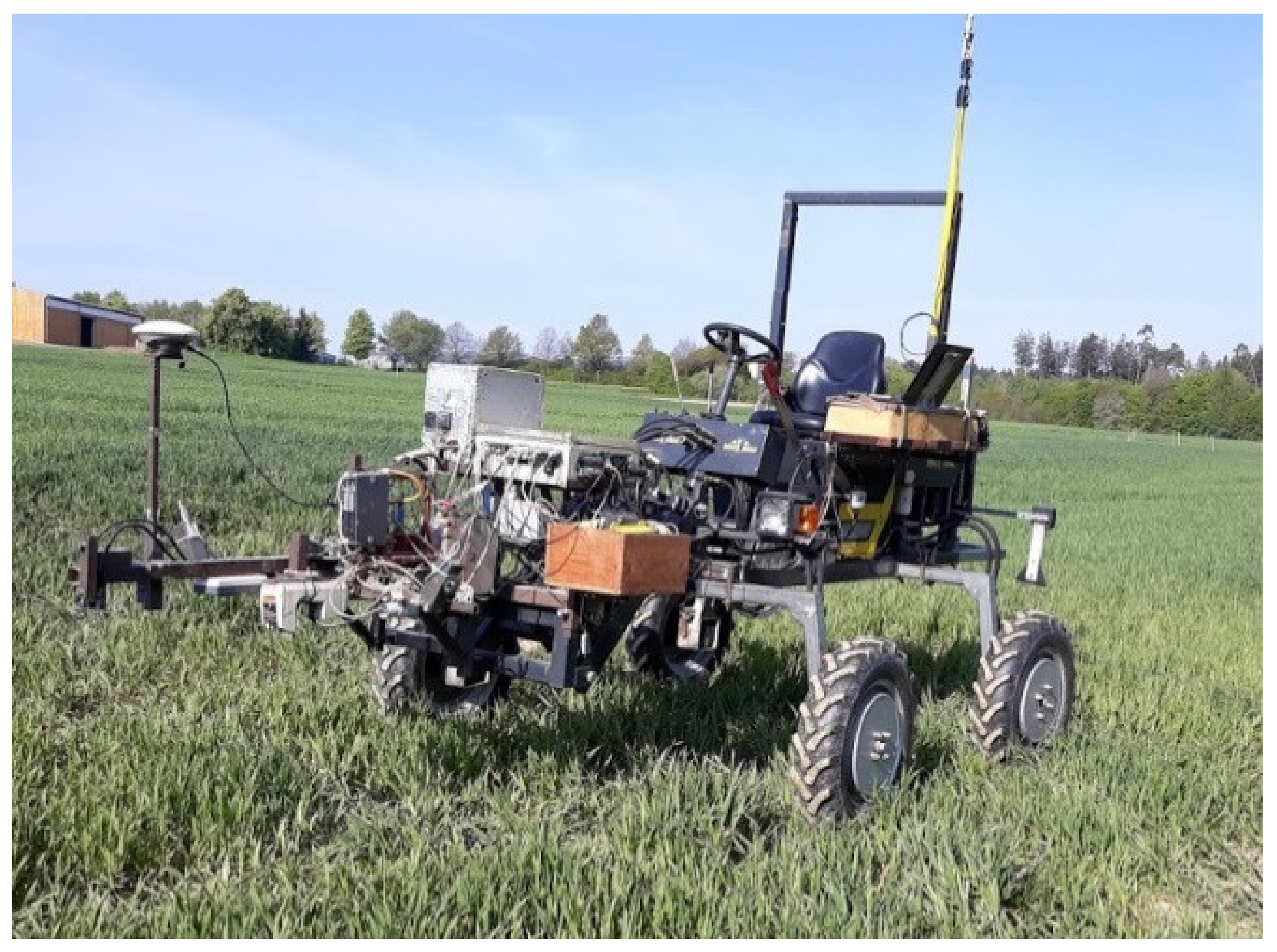
| Crop Circle ACS-470 (vehicle-carried) | Active | Holland Scientific, Inc, Lincoln, NE | 670 (Red), 730 (Red edge), and 760 nm (near-infrared; NIR) | Oval of ~32° by ~6°: 0.600 × 0.112 m (0.0527 m2) |
| Greenseeker RT100 (vehicle-carried) | Active | NTech Industries, Inc., Ukiah, CA | 656 (Red) and 774 nm (NIR) | Rectangle of 0.69 × 0.015 m (0.010 m2) |
| UAV senseFly eBee | Passive | Sensefly, Cheseaux, Switzerland | 530–570 (Green), 640–680 (Red), 730–740 (Red edge), 770–818 (NIR) | Horizontally 61.9°, vertically 48.5°, diagonally 73.7° |
| HandySpec Field (handheld) | Passive | tec5, Oberursel, Germany | Nominal resolution of 2 nm between 302 and 1148 nm | Circle with 12° aperture (0.02 m2) |
| Hyperspectral bidirectional passive spectrometer (vehicle-carried) | Passive | tec5, Oberursel, Germany | Nominal resolution of 3.3 nm between 300 and 1000 nm | Circle with 22° aperture (0.021 m2) |
| Spectral Reflectance Indices | Formula | Reference |
|---|---|---|
| Normalized Difference Vegetation Index (NDVI) | NIR−Red/NIR+Red | (Sellers, 1985) [32] |
| Green Normalized Difference Vegetation Index (GNDVI) | NIR−Green/NIR+Green | (Ma et al., 1996) [33] |
| Red Ratio of Vegetation Index | NIR/Red | (Birth and McVey, 1968) [34] |
| Green Ratio of Vegetation Index | NIR/Green | (Birth and McVey, 1968) [34] |
| Red Edge Ratio of Vegetation Index | NIR/Red edge | (Gitelson et al., 2003) [35] |
| Water Index | R900/R970 | (Peñuelas et al., 1993) [36] |
| Red Edge/Red Ratio | Red edge/Red | (Kipp et al., 2014) [26] |
| Red Edge Inflection Point (REIP) | 700 + 40 × [(R670 + R780)/2−R700)/(R740−R700)] | (Guyot et al., 1988) [37] |
| Sensor | Date (dd-mm-yyyy) | Index | n | 9:00 Versus 14:00 h | 9:00 Versus 16:00 h | 14:00 Versus 16:00 h | |||
|---|---|---|---|---|---|---|---|---|---|
| 9:00 h | 14:00 h | 9:00 h | 16:00 h | 14:00 h | 16:00 h | ||||
| Crop Circle ACS-470 † | 07-05-2019 | Red edge/Red | 320 | 2.47 | 2.19 | 2.47 | 2.24 | 2.19 | 2.24 |
| NIR/Red edge | 320 | 1.99 | 2.10 | 1.99 | 2.01 | 2.10 | 2.01 | ||
| NIR/Red | 320 | 5.07 | 4.78 | 5.07 | 4.70 | 4.78 | 4.70 | ||
| NDVI | 320 | 0.638 | 0.615 | 0.638 | 0.608 | 0.615 | 0.608 | ||
| 03-06-2019 | Red edge/Red | 230 | 2.07 | 1.85 | 2.07 | 1.92 | 1.85 | 1.92 | |
| NIR/Red edge | 230 | 2.67 | 2.81 | 2.67 | 2.76 | 2.8 | 2.76 | ||
| NIR/Red | 230 | 5.63 | 5.34 | 5.63 | 5.42 | 5.34 | 5.42 | ||
| NDVI | 230 | 0.674 | 0.654 | 0.674 | 0.657 | 0.654 | 0.657 | ||
| 27-06-2019 | Red edge/Red | 313 | 1.96 | 1.92 | 1.96 | 1.95 | 1.92 | 1.95 | |
| NIR/Red edge | 313 | 2.15 | 2.10 | 2.15 | 2.09 | 2.10 | 2.09 | ||
| NIR/Red | 313 | 4.27 | 4.10 | 4.27 | 4.13 | 4.10 | 4.13 | ||
| NDVI | 313 | 0.602 | 0.590 | 0.602 | 0.591 | 0.590 | 0.591 | ||
| Greenseeker RT100 ɸ | 07-05-2019 | NIR/Red | 160 | 6.29 | 5.72 | 6.29 | 6.10 | 5.72 | 6.10 |
| NDVI | 160 | 0.694 | 0.678 | 0.694 | 0.691 | 0.678 | 0.691 | ||
| 03-06-2019 | NIR/Red | 201 | 5.74 | 5.13 | 5.74 | 7.15 | 5.13 | 7.15 | |
| NDVI | 201 | 0.681 | 0.650 | 0.681 | 0.730 | 0.650 | 0.730 | ||
| 27-06-2019 | NIR/Red | 313 | 5.56 | 5.36 | 5.56 | 5.27 | 5.36 | 5.27 | |
| NDVI | 313 | 0.681 | 0.671 | 0.681 | 0.668 | 0.671 | 0.669 | ||
| Date (dd-mm-yyyy) | Index | n | 9:00 Versus 14:00 h | 9:00 Versus 16:00 h | 14:00 Versus 16:00 h | |||
|---|---|---|---|---|---|---|---|---|
| 9:00 h | 14:00 h | 9:00 h | 16:00 h | 14:00 h | 16:00 h | |||
| 07-05-2019 | NDVI | 320 | No data | No data | 0.835 | 0.843 | ||
| GNDVI | 320 | No data | No data | 0.762 | 0.763 | |||
| NIR/Green | 320 | No data | No data | 8.10 | 7.99 | |||
| NIR/Red | 320 | No data | No data | 13.25 | 13.41 | |||
| NIR/Red edge | 320 | No data | No data | 1.61 | 1.70 | |||
| Red edge/Red | 320 | No data | No data | 7.90 | 7.66 | |||
| 03-06-2019 | NDVI | 320 | 0.894 | 0.841 | 0.894 | 0.886 | 0.841 | 0.886 |
| GNDVI | 320 | 0.821 | 0.790 | 0.821 | 0.793 | 0.790 | 0.793 | |
| NIR/Green | 320 | 10.63 | 8.86 | 10.63 | 8.99 | 8.86 | 8.99 | |
| NIR/Red | 320 | 19.38 | 12.46 | 19.38 | 17.56 | 12.46 | 17.56 | |
| NIR/Red edge | 320 | 1.94 | 1.75 | 1.94 | 1.85 | 1.75 | 1.85 | |
| Red edge/Red | 320 | 9.88 | 7.05 | 9.88 | 9.39 | 7.05 | 9.39 | |
| 27-06-2019 | NDVI | 312 | 0.821 | 0.781 | 0.821 | 0.800 | 0.781 | 0.800 |
| GNDVI | 312 | 0.744 | 0.716 | 0.744 | 0.730 | 0.716 | 0.730 | |
| NIR/Green | 312 | 6.96 | 6.24 | 6.96 | 6.55 | 6.24 | 6.55 | |
| NIR/Red | 312 | 10.59 | 8.62 | 10.5 | 9.37 | 8.62 | 9.37 | |
| NIR/Red edge | 312 | 1.76 | 1.69 | 1.76 | 1.72 | 1.69 | 1.72 | |
| Red edge/Red | 312 | 5.96 | 5.06 | 5.96 | 5.41 | 5.06 | 5.41 | |
| Date (dd-mm-yyyy) | Index | n | 9:00 Versus 14:00 h | 9:00 Versus 16:00 h | 14:00 Versus 16:00 h | |||
|---|---|---|---|---|---|---|---|---|
| 9:00 h | 14:00 h | 9:00 h | 16:00 h | 14:00 h | 16:00 h | |||
| 07-05-2019 | NIR/Green | 293 | 9.63 | 8.43 | 9.63 | 8.65 | 8.43 | 8.65 |
| NIR/Red | 293 | 28.55 | 19.65 | 28.55 | 22.22 | 19.65 | 22.22 | |
| NIR/Red edge | 293 | 1.68 | 1.66 | 1.68 | 1.67 | 1.66 | 1.67 | |
| Water index | 293 | 1.176 | 1.160 | 1.176 | 1.167 | 1.160 | 1.167 | |
| REIP | 293 | 723.66 | 723.80 | 723.66 | 723.77 | 723.80 | 723.77 | |
| 03-06-2019 | NIR/Green | 320 | 12.16 | 11.99 | 12.16 | 12.92 | 11.99 | 12.92 |
| NIR/Red | 320 | 29.95 | 26.70 | 29.95 | 29.96 | 26.70 | 29.96 | |
| NIR/Red edge | 320 | 2.03 | 2.05 | 2.03 | 2.07 | 2.05 | 2.07 | |
| Water index | 320 | 1.34 | 1.35 | 1.34 | 1.35 | 1.35 | 1.35 | |
| REIP | 320 | 728.78 | 729.39 | 728.78 | 729.40 | 729.39 | 729.40 | |
| 27-06-2019 | NIR/Green | 313 | 6.53 | 6.63 | 6.53 | 6.62 | 6.63 | 6.62 |
| NIR/Red | 313 | 13.02 | 12.68 | 13.02 | 12.9 | 12.68 | 12.90 | |
| NIR/Red edge | 313 | 1.66 | 1.66 | 1.66 | 1.65 | 1.66 | 1.65 | |
| Water index | 313 | 1.29 | 1.27 | 1.29 | 1.25 | 1.27 | 1.25 | |
| REIP | 313 | 725.03 | 725.12 | 725.03 | 724.98 | 725.12 | 724.98 | |
| Date (dd-mm-yyyy) | Index | n | 9:00 Versus 14:00 h | 9:00 Versus 16:00 h | 14:00 Versus 16:00 h | |||
|---|---|---|---|---|---|---|---|---|
| 9:00 h | 14:00 h | 9:00 h | 16:00 h | 14:00 h | 16:00 h | |||
| 07-05-2019 | NDVI | 320 | 0.911 | 0.852 | 0.911 | 0.880 | 0.851 | 0.880 |
| GNDVI | 320 | 0.794 | 0.747 | 0.794 | 0.767 | 0.747 | 0.767 | |
| NIR/Red | 320 | 29.76 | 17.49 | 29.76 | 21.60 | 17.49 | 21.60 | |
| NIR/Green | 320 | 9.73 | 7.83 | 9.73 | 8.49 | 7.83 | 8.49 | |
| NIR/Red edge | 320 | 1.79 | 1.72 | 1.79 | 1.76 | 1.72 | 1.76 | |
| Red edge/Red | 320 | 15.93 | 9.73 | 15.93 | 11.80 | 9.73 | 11.80 | |
| Water index | 320 | 1.122 | 1.125 | 1.122 | 1.139 | 1.125 | 1.139 | |
| REIP | 320 | 725.95 | 725.38 | 725.95 | 725.78 | 725.38 | 725.78 | |
| 03-06-2019 | NDVI | 315 | 0.931 | 0.921 | 0.931 | 0.933 | 0.921 | 0.933 |
| GNDVI | 315 | 0.839 | 0.843 | 0.839 | 0.848 | 0.843 | 0.848 | |
| NIR/Red | 315 | 31.99 | 30.76 | 31.99 | 34.35 | 30.76 | 34.35 | |
| NIR/Green | 315 | 12.12 | 12.85 | 12.12 | 13.03 | 12.85 | 13.03 | |
| NIR/Red edge | 315 | 2.19 | 2.25 | 2.19 | 2.23 | 2.25 | 2.23 | |
| Red edge/Red | 315 | 14.42 | 13.15 | 14.42 | 15.76 | 13.15 | 15.76 | |
| Water index | 315 | 1.295 | 1.320 | 1.295 | 1.314 | 1.320 | 1.314 | |
| REIP | 315 | 731.51 | 732.45 | 731.51 | 732.09 | 732.45 | 732.09 | |
| 27-06-2019 | NDVI | 305 | 0.852 | 0.841 | 0.852 | 0.844 | 0.841 | 0.844 |
| GNDVI | 305 | 0.751 | 0.729 | 0.751 | 0.723 | 0.729 | 0.723 | |
| NIR/Red | 305 | 13.46 | 12.91 | 13.46 | 12.94 | 12.91 | 12.94 | |
| NIR/Green | 305 | 7.33 | 6.71 | 7.33 | 6.49 | 6.71 | 6.49 | |
| NIR/Red edge | 305 | 1.77 | 1.76 | 1.77 | 1.75 | 1.76 | 1.75 | |
| Red edge/Red | 305 | 7.48 | 7.33 | 7.48 | 7.25 | 7.33 | 7.25 | |
| Water index | 305 | 1.268 | 1.253 | 1.268 | 1.252 | 1.253 | 1.252 | |
| REIP | 305 | 727.94 | 727.41 | 727.94 | 727.21 | 727.41 | 727.21 | |
| Sensor | Index | N | 9:00 h Sunny | 9:00 h Overcast |
|---|---|---|---|---|
| Crop Circle ACS-470 | Red edge/Red | 320 | 2.33 | 2.47 |
| NIR/Red edge | 320 | 2.00 | 1.99 | |
| NIR/Red | 320 | 4.82 | 5.07 | |
| NDVI | 320 | 0.621 | 0.638 | |
| Greenseeker RT100 | NIR/Red | 160 | 6.74 | 6.29 |
| NDVI | 160 | 0.69 | 0.694 | |
| Bidirectional spectrometer | NIR/Green | 293 | 8.44 | 9.63 |
| NIR/Red | 293 | 20.19 | 28.55 | |
| NIR/Red edge | 293 | 1.65 | 1.68 | |
| Water index | 293 | 1.146 | 1.176 | |
| REIP | 293 | 723.4 | 723.66 | |
| HandySpec Field Sensor | NDVI | 320 | 0.873 | 0.911 |
| GNDVI | 320 | 0.765 | 0.794 | |
| NIR/Red | 320 | 19.47 | 29.76 | |
| NIR/Green | 320 | 8.34 | 9.73 | |
| NIR/Red edge | 320 | 1.74 | 1.79 | |
| Red edge/Red | 320 | 10.77 | 15.93 | |
| Water index | 320 | 1.13 | 1.12 | |
| REIP | 320 | 725.56 | 725.95 |
Publisher’s Note: MDPI stays neutral with regard to jurisdictional claims in published maps and institutional affiliations. |
© 2021 by the authors. Licensee MDPI, Basel, Switzerland. This article is an open access article distributed under the terms and conditions of the Creative Commons Attribution (CC BY) license (https://creativecommons.org/licenses/by/4.0/).
Share and Cite
de Souza, R.; Buchhart, C.; Heil, K.; Plass, J.; Padilla, F.M.; Schmidhalter, U. Effect of Time of Day and Sky Conditions on Different Vegetation Indices Calculated from Active and Passive Sensors and Images Taken from UAV. Remote Sens. 2021, 13, 1691. https://0-doi-org.brum.beds.ac.uk/10.3390/rs13091691
de Souza R, Buchhart C, Heil K, Plass J, Padilla FM, Schmidhalter U. Effect of Time of Day and Sky Conditions on Different Vegetation Indices Calculated from Active and Passive Sensors and Images Taken from UAV. Remote Sensing. 2021; 13(9):1691. https://0-doi-org.brum.beds.ac.uk/10.3390/rs13091691
Chicago/Turabian Stylede Souza, Romina, Claudia Buchhart, Kurt Heil, Jürgen Plass, Francisco M. Padilla, and Urs Schmidhalter. 2021. "Effect of Time of Day and Sky Conditions on Different Vegetation Indices Calculated from Active and Passive Sensors and Images Taken from UAV" Remote Sensing 13, no. 9: 1691. https://0-doi-org.brum.beds.ac.uk/10.3390/rs13091691