
Simultaneous Time-Varying Vibration and Nonlinearity Compensation for One-Period Triangular-FMCW Lidar Signal

 , , and
Abstract
:
1. Introduction
2. Analysis of Ranging Principle for FMCW Lidar
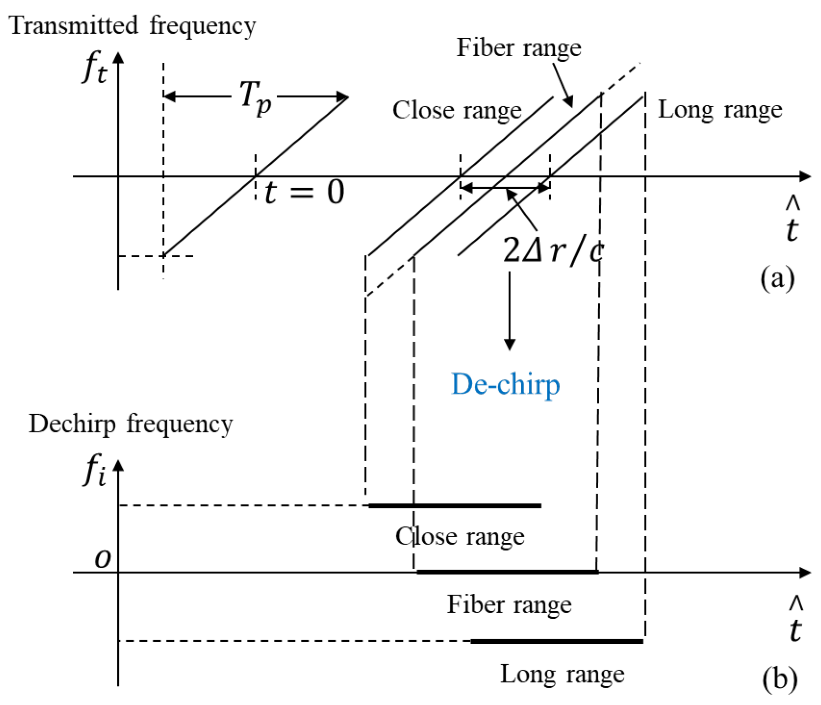
2.1. Ideal Coherent Detection Process
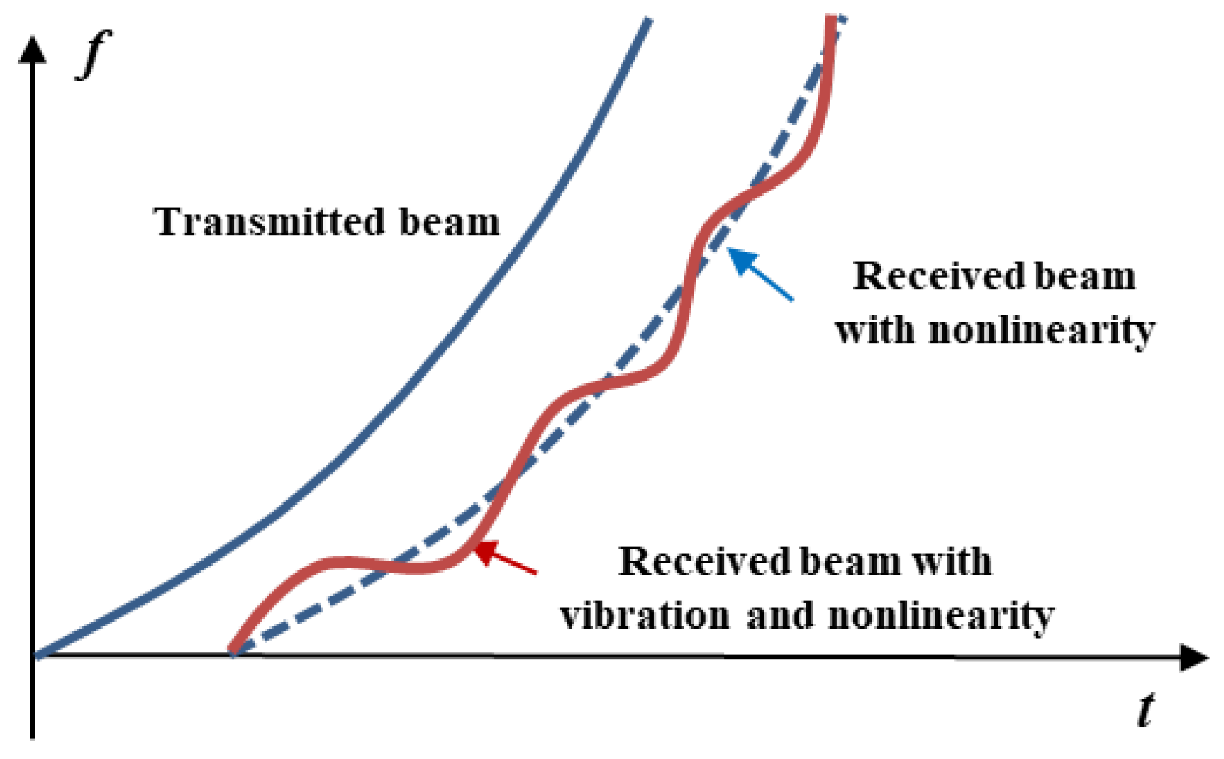
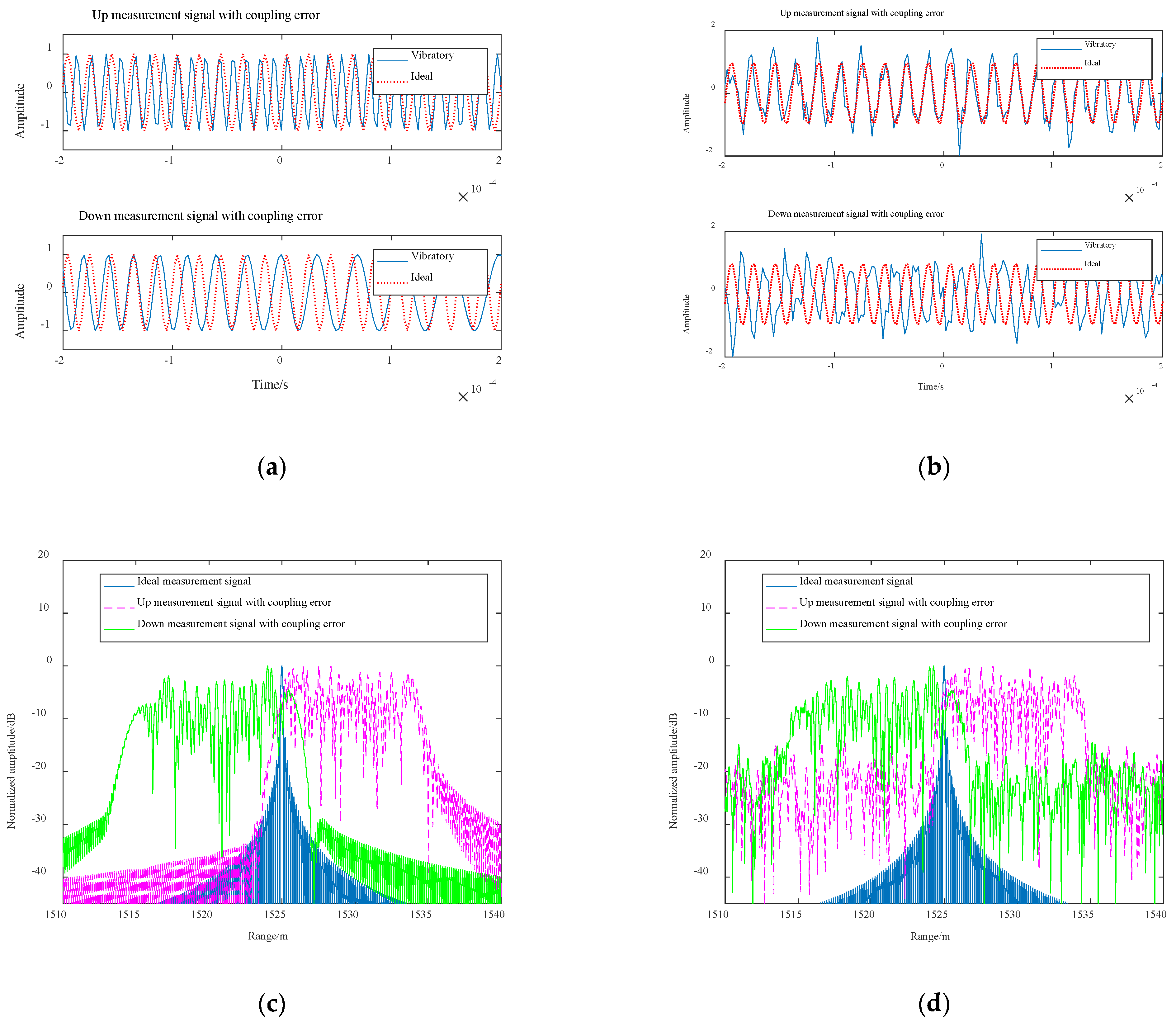
2.2. Impact of Vibration Coupled with Nonlinearity on FMCW Lidar Ranging
3. Time-Varying Vibration and Nonlinearity Compensation Method
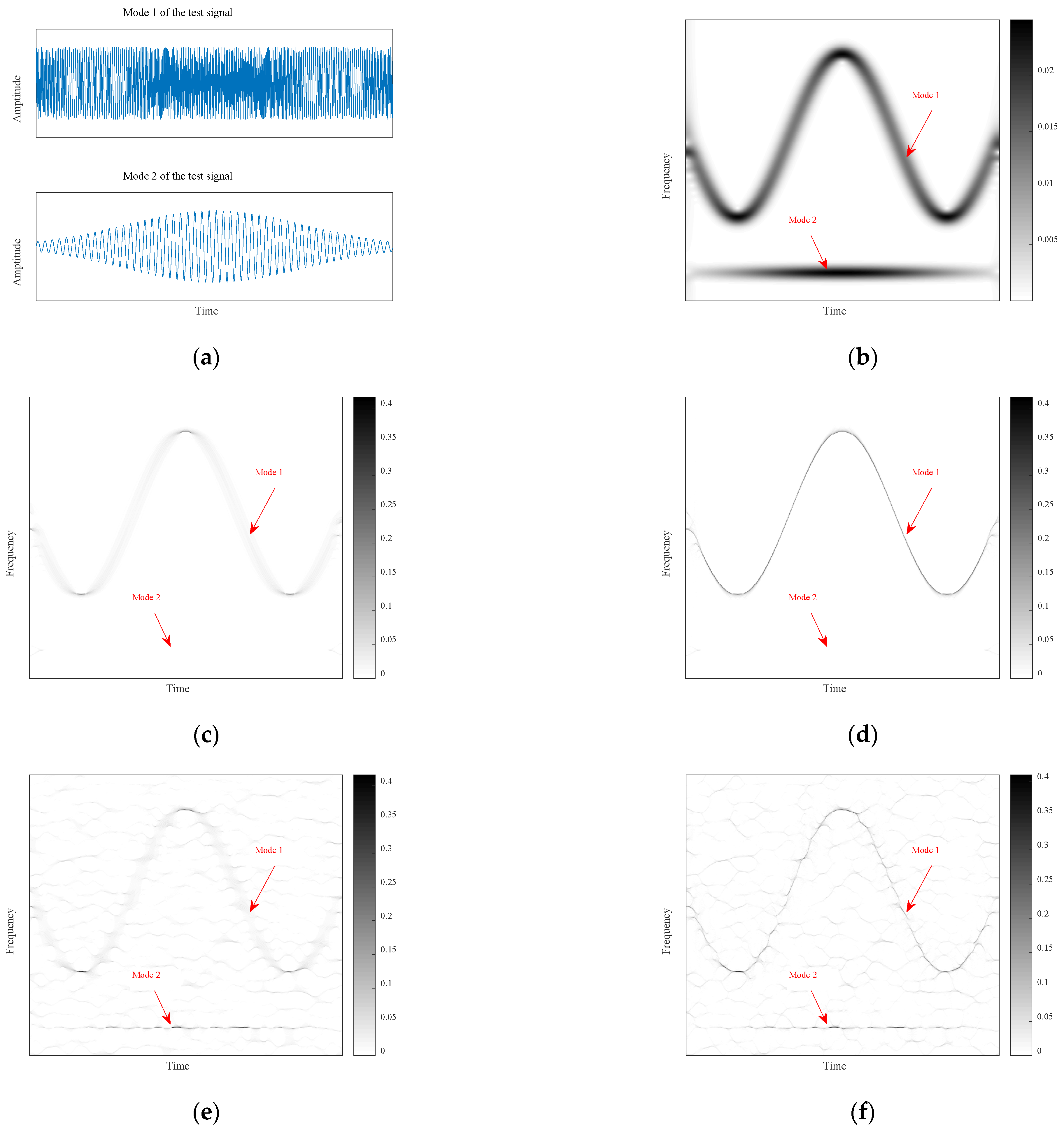
3.1. Instantaneous Ranging Model Based on Second-Order SST
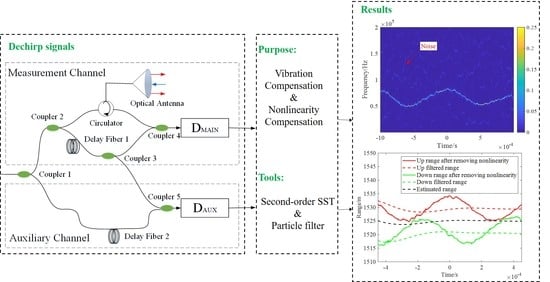
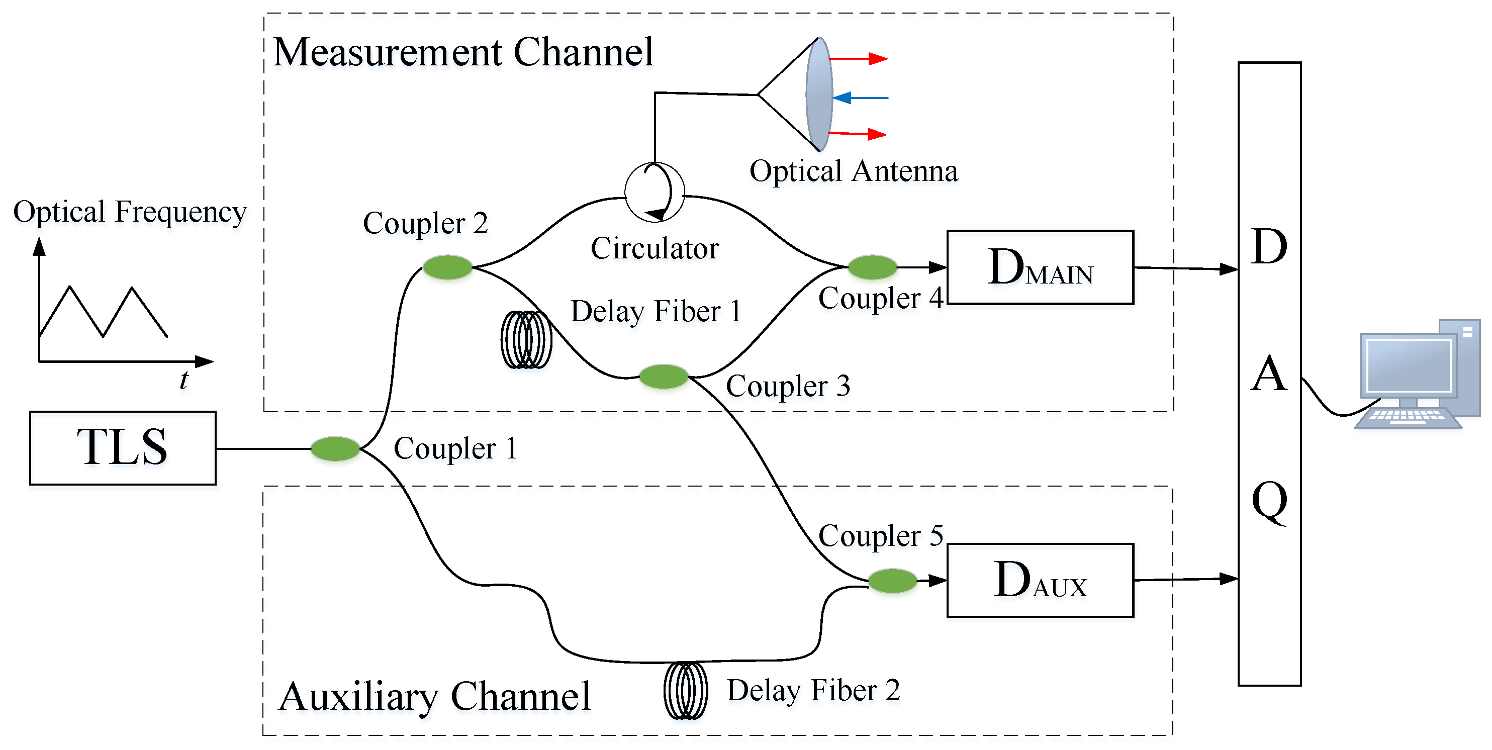
3.2. Lidar System Design and Time-Varying Vibration and Nonlinearity Compensation Method
3.3. Workflow of the Proposed Method
- (a):
- Extract up and down dechirp signals from one-period T-FMCW Lidar signals. The up and down measurement dechirp signals obtained from the measurement channel are denoted as and , respectively. The up and down reference dechirp signals obtained from the auxiliary channel are denoted as and , respectively.
- (b):
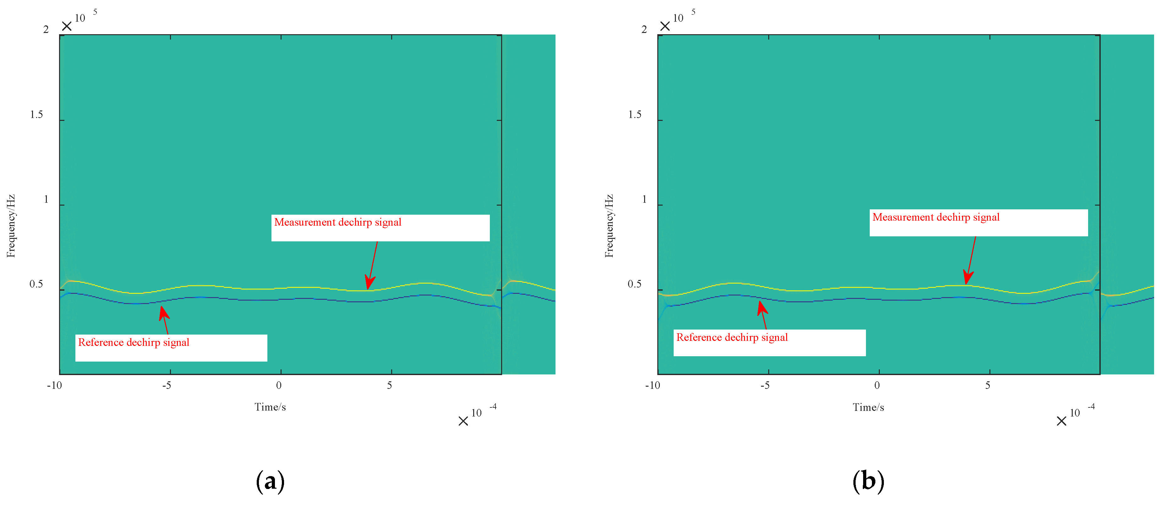
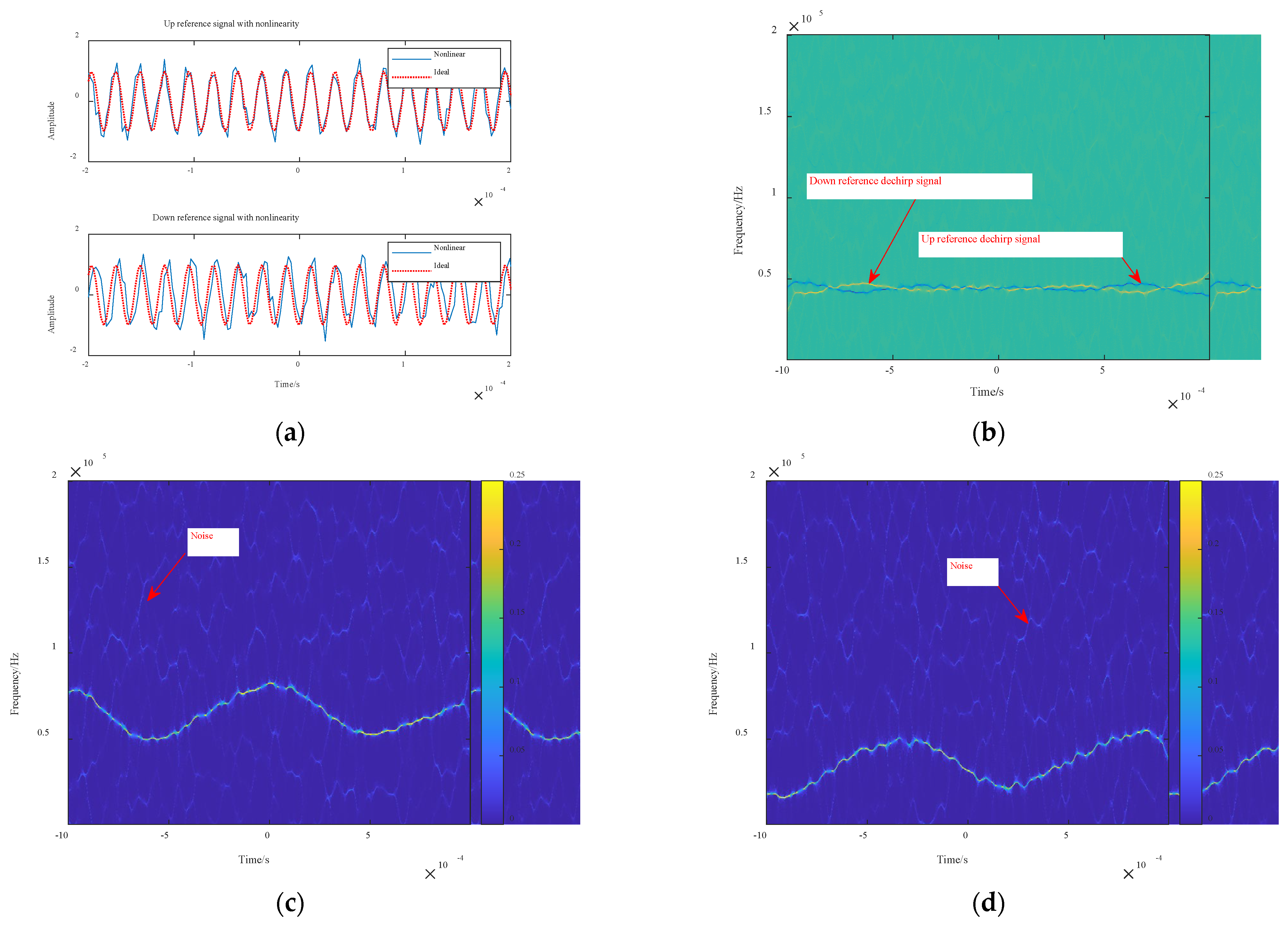
- Calculate the second-order modulation operators and the estimation operator of second-order instantaneous frequency for reference dechirp signals and measurement dechirp signals by using Equations (19) and (20), and determine the criterion of energy rearrangement.
- (c):
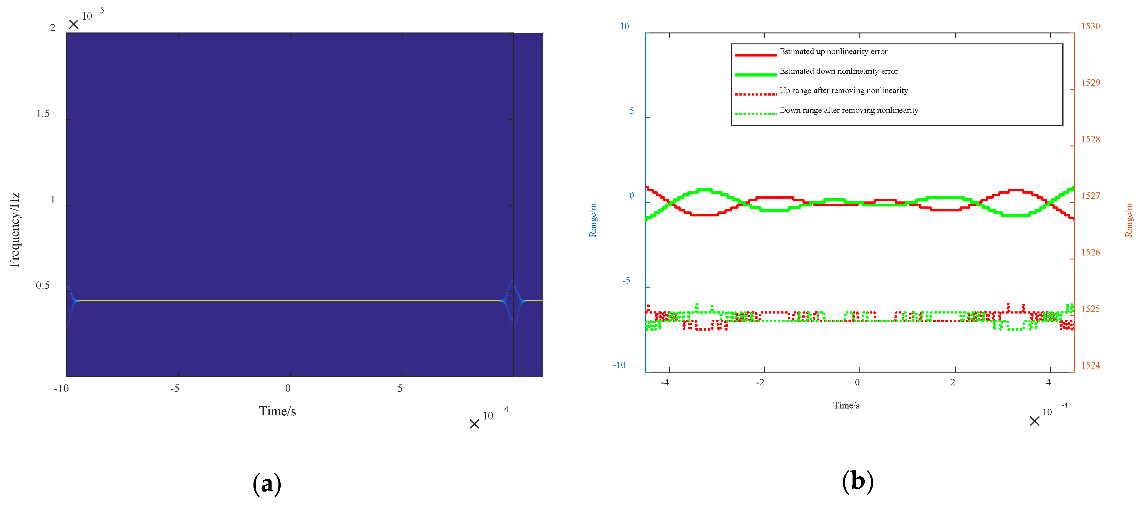
- Rearrange the time-varying spectrums by using the second-order estimation operator and obtain the squeezing results by using Equation (21).
- (d):
- Extract central time-frequency curves based on the ridge detection method. The time-frequency curves of the up and down measurement dechirp signals are denoted as and, respectively. The time-frequency curves of the up and down reference dechirp signals are denoted as and , respectively.
- (e):
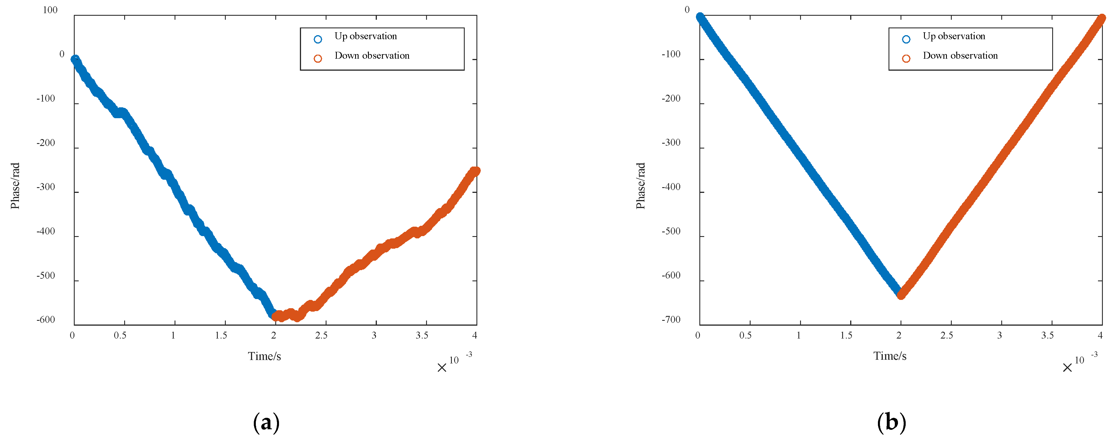
- Calculate the instantaneous measurement ranges and corresponding to and , and the instantaneous reference ranges and corresponding to and by using Equation (23).
- (f):
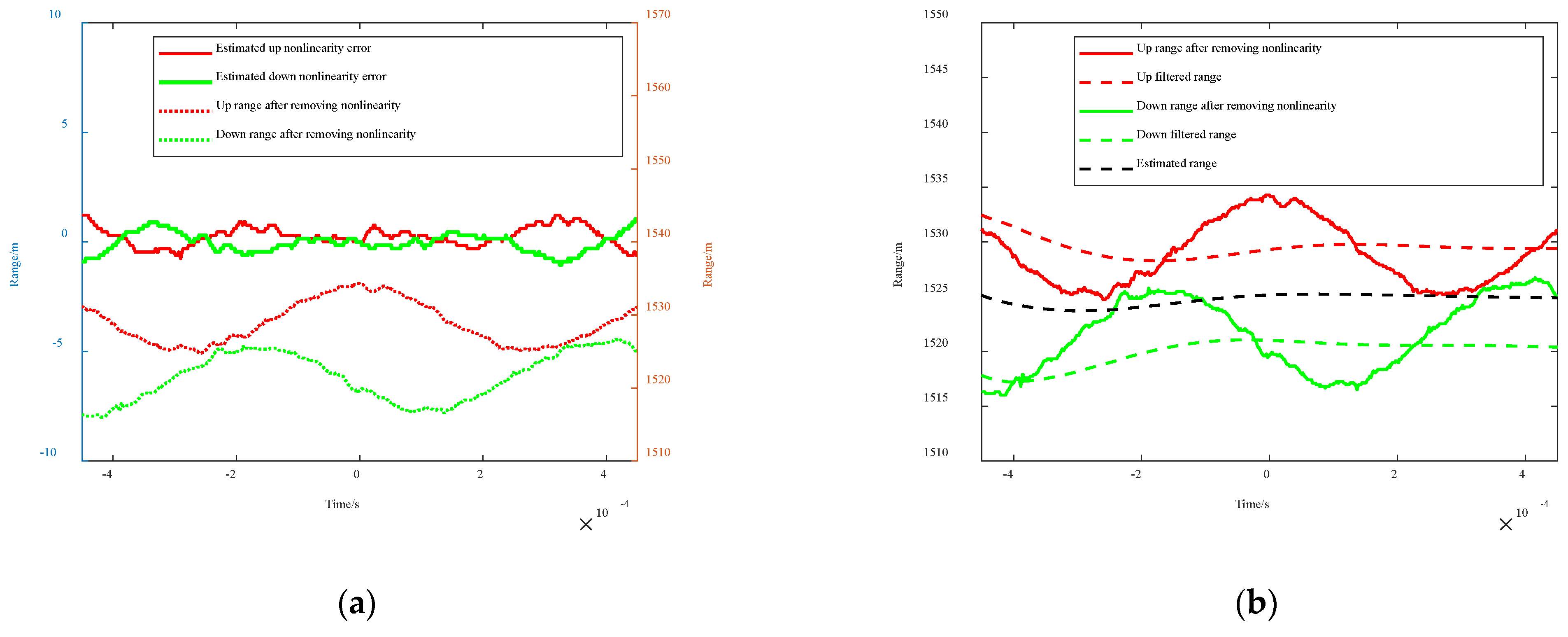
- Estimate the nonlinearity errors and of up and down observations by using and according to Equation (25), and eliminate and from the instantaneous measurement ranges and. The instantaneous ranges after preliminarily compensating for the nonlinearity errors are denoted as and .
- (g):
- Construct the state function and measurement function of and using Equations (28) and (29).
- (h):
- Establish the PF model for T-FMCW, and compensate for the disturbance errors and the residual nonlinearity errors by applying PF to and .
- (i):
- Substitute the filtered ranges into Equation (34) to estimate the actual range of target.
4. Experimental Analysis
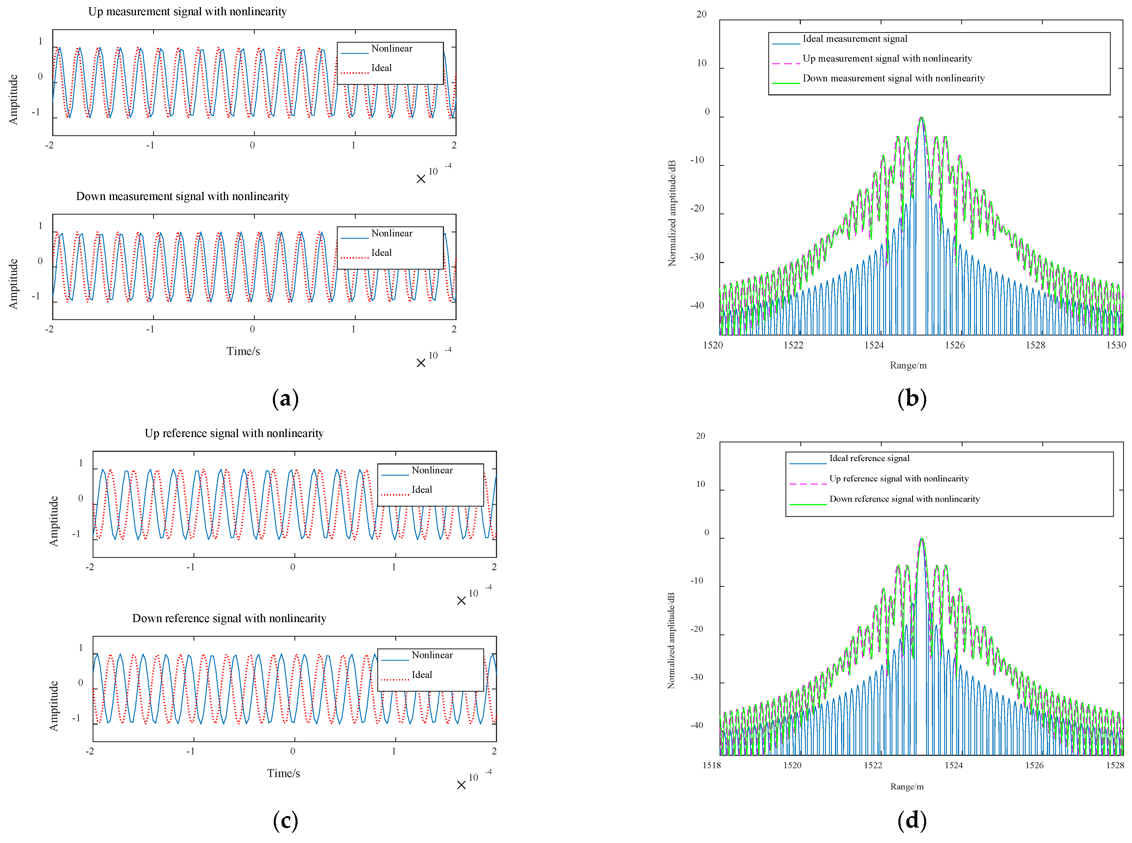
4.1. Prove the Validity of the Proposed Method with Nonlinearity
4.2. Prove the Validity of the Proposed Method with Coupling Error
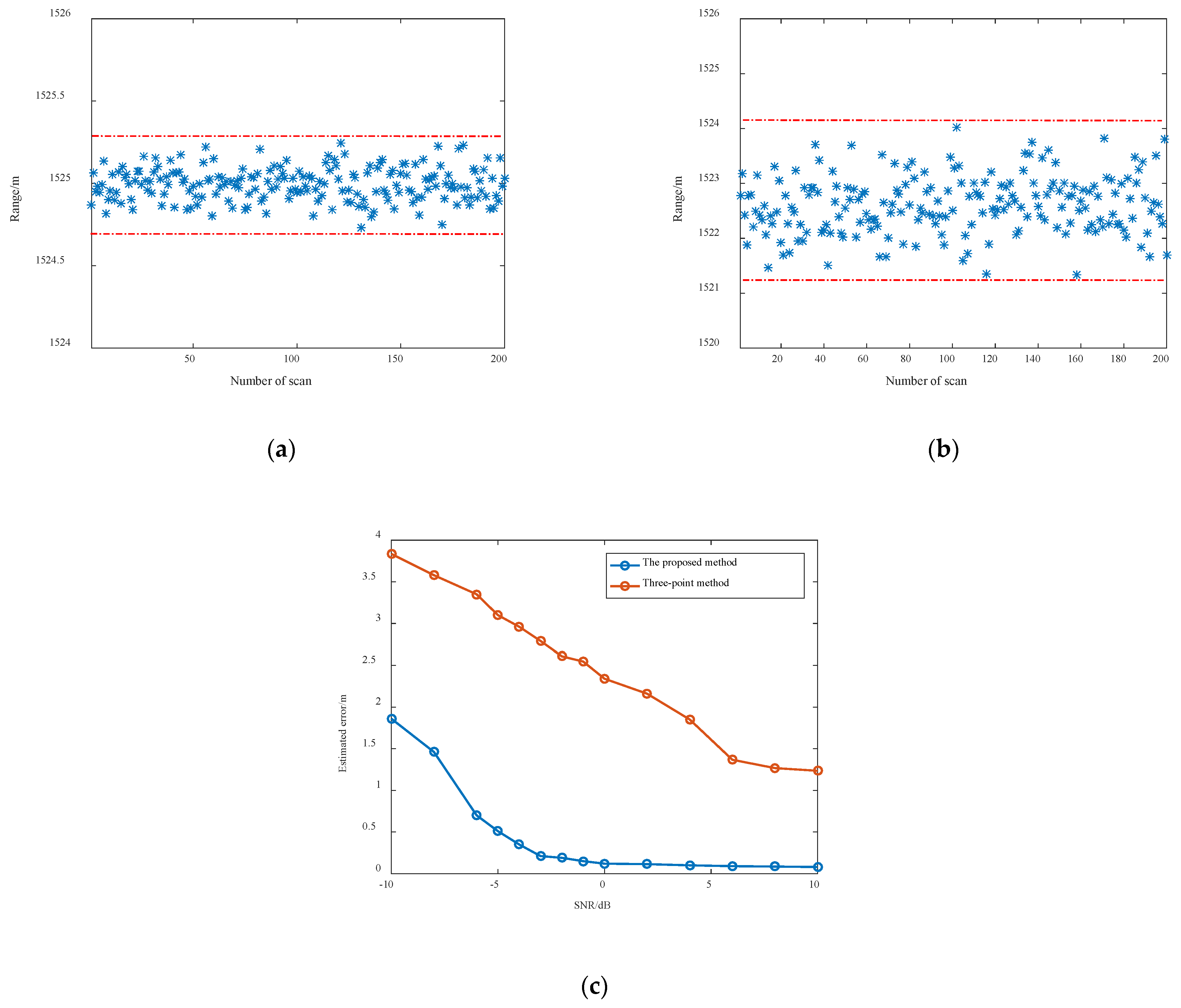
4.3. Compare the Ranging Performance with Traditional Three-Point Method
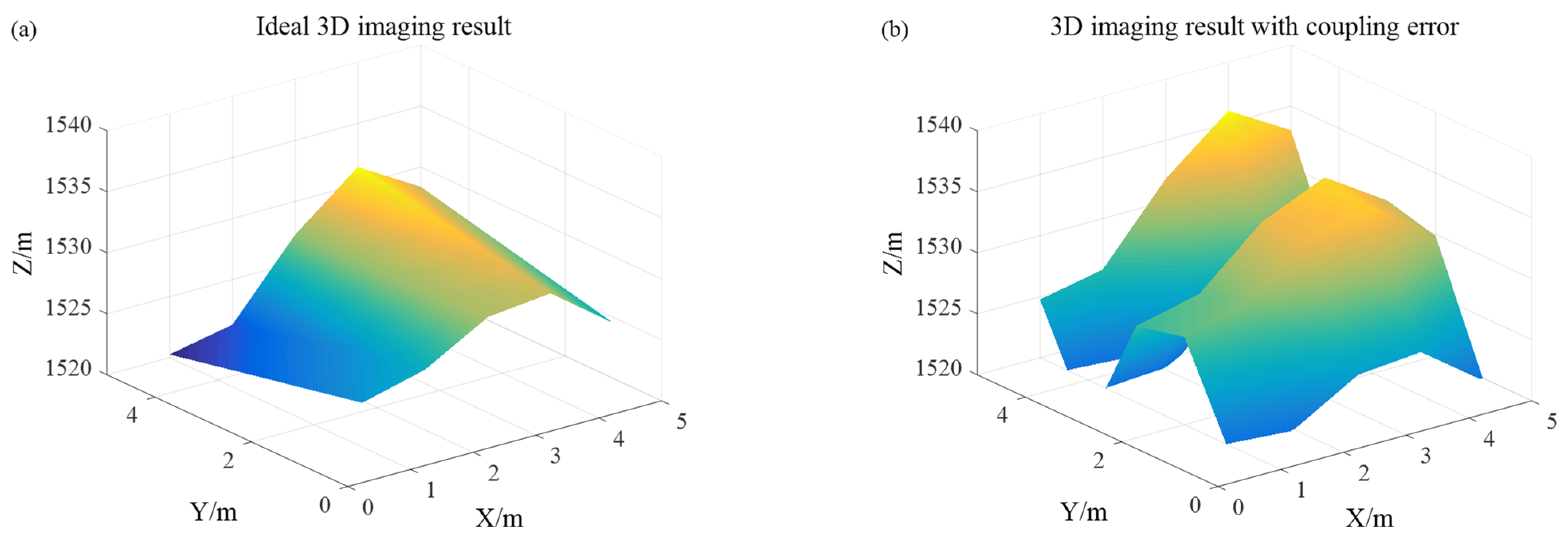
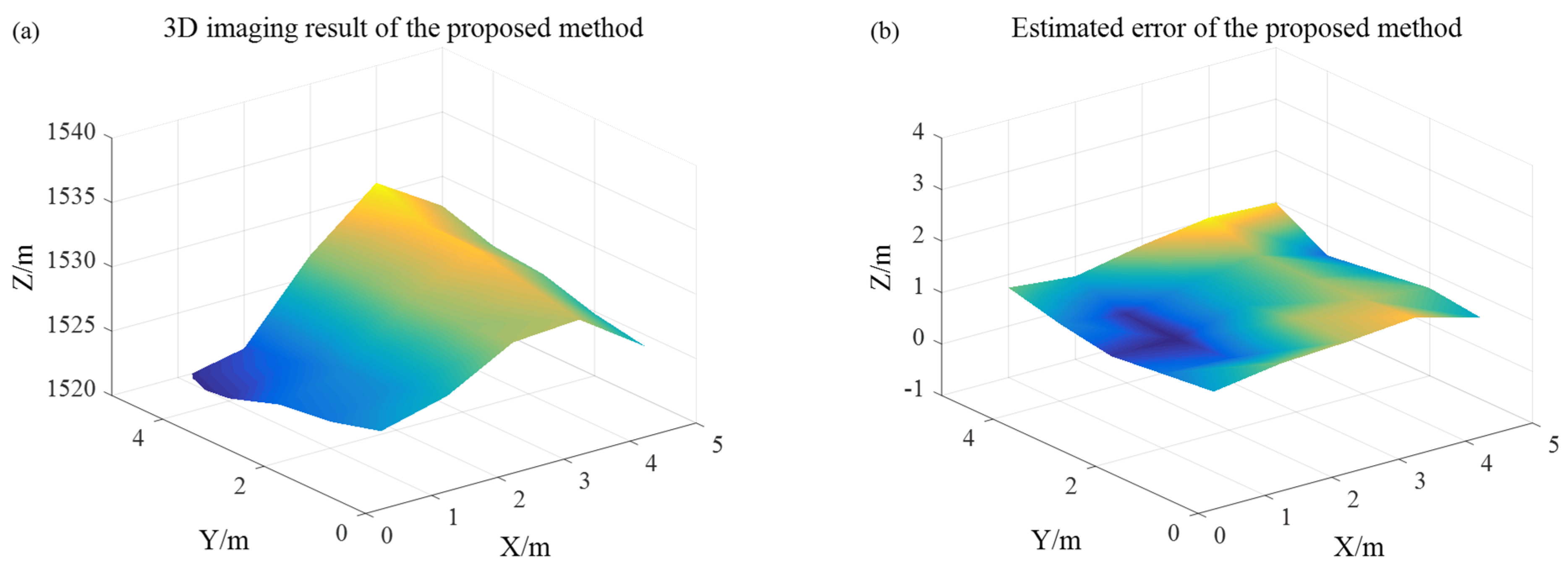
4.4. Prove the Applicability of the Proposed Method to 3D Imaging
5. Discussion
6. Conclusions
Author Contributions
Funding
Institutional Review Board Statement
Informed Consent Statement
Data Availability Statement
Acknowledgments
Conflicts of Interest
Abbreviations
| FMCW | Frequency modulation continuous wave |
| T-FMCW | Triangular FMCW |
| second-order SST | Second-order synchrosqueezing transform |
| PF | Particle filtering |
| 3D | Three dimensional |
References
- Moore, E.D.; McLeod, R.R. Correction of sampling errors due to laser tuning rate fluctuations in swept-wavelength interferometry. Opt. Express 2008, 16, 13139–13149. [Google Scholar] [CrossRef]
- Gao, S.; Hui, R. Frequency-modulated continuous-wave lidar using I/Q modulator for simplified heterodyne detection. Opt. Lett. 2012, 37, 2022–2024. [Google Scholar] [CrossRef] [PubMed] [Green Version]
- Batet, O.; Dios, F.; Comeron, A.; Agishev, R.R. Intensity-modulated linear-frequency-modulated continuous-wave lidar for distributed media: fundamentals of technique. Appl. Opt. 2010, 49, 3369–3379. [Google Scholar] [CrossRef]
- Redman, B.; Ruff, W.; Stann, B.; Giza, M.; Lawler, W.; Dammann, J.; Potter, W. Anti-ship missile tracking with a chirped AM ladar—Update: Design, model predictions, and experimental results. Def. Secur. 2005, 5791, 330–341. [Google Scholar] [CrossRef]
- Karlsson, C.J.; Olsson, F.Å.A. Linearization of the frequency sweep of a frequency-modulated continuous-wave semiconductor laser radar and the resulting ranging performance. Appl. Opt. 1999, 38, 3376–3386. [Google Scholar] [CrossRef] [PubMed]
- Beck, S.M.; Buck, J.R.; Buell, W.F.; Dickinson, R.P.; Kozlowski, D.A.; Marechal, N.J.; Wright, T.J. Synthetic-aperture imaging laser radar: laboratory demonstration and signal processing. Appl. Opt. 2005, 44, 7621–7629. [Google Scholar] [CrossRef]
- Roos, P.A.; Reibel, R.R.; Berg, T.; Kaylor, B.; Barber, Z.W.; Babbitt, W.R. Ultrabroadband optical chirp linearization for precision metrology applications. Opt. Lett. 2009, 34, 3692–3694. [Google Scholar] [CrossRef]
- Kakuma, S.; Katase, Y. Frequency scanning interferometry immune to length drift using a pair of vertical-cavity surface-emitting laser diodes. Opt. Rev. 2012, 19, 376–380. [Google Scholar] [CrossRef]
- Krause, B.W.; Tiemann, B.G.; Gatt, P. Motion compensated frequency modulated continuous wave 3D coherent imaging ladar with scannerless architecture. Appl. Opt. 2012, 51, 8745–8761. [Google Scholar] [CrossRef]
- Yang, H.-J.; Nyberg, S.; Riles, K. High-precision absolute distance measurement using dual-laser frequency scanned interferometry under realistic conditions. Nucl. Instrum. Methods Phys. Res. Sect A Accel. Spectrom. Detect. Assoc. Equip. 2007, 575, 395–401. [Google Scholar] [CrossRef] [Green Version]
- Martinez, J.J.; Campbell, M.A.; Warden, M.S.; Hughes, E.B.; Copner, N.J.; Lewis, A.J. Dual-Sweep Frequency Scanning Interferometry Using Four Wave Mixing. IEEE Photon Technol. Lett. 2015, 27, 733–736. [Google Scholar] [CrossRef]
- Swinkels, B.L.; Bhattacharya, N.; Braat, J.J. Correcting movement errors in frequency-sweeping interferometry. Opt. Lett. 2005, 30, 2242–2244. [Google Scholar] [CrossRef] [Green Version]
- Tao, L.; Liu, Z.; Zhang, W.; Zhou, Y. Frequency-scanning interferometry for dynamic absolute distance measurement using Kalman filter. Opt. Lett. 2014, 39, 6997–7000. [Google Scholar] [CrossRef] [PubMed]
- Jia, X.; Liu, Z.; Tao, L.; Deng, Z.; Deng, L.T.A.Z. Frequency-scanning interferometry using a time-varying Kalman filter for dynamic tracking measurements. Opt. Express 2017, 25, 25782. [Google Scholar] [CrossRef] [PubMed]
- Guo, L.; Huang, Y.; Li, X.; Zeng, X.; Xing, M. A Novel 3-D Imaging Configuration Exploiting Synthetic Aperture Ladar. Curr. Opt. Photon. 2017, 1, 598–603. [Google Scholar] [CrossRef]
- Pierrottet, D.; Amzajerdian, F.; Petway, L.; Barnes, B.; Lockard, G.; Rubio, M. Linear FMCW Laser Radar for Precision Range and Vector Velocity Measurements. MRS Online Proc. Libr. 2008, 1076. [Google Scholar] [CrossRef] [Green Version]
- Ahn, T.-J.; Lee, J.Y.; Kim, D.Y. Suppression of nonlinear frequency sweep in an optical frequency-domain reflectometer by use of Hilbert transformation. Appl. Opt. 2005, 44, 7630–7634. [Google Scholar] [CrossRef]
- Ahn, T.-J.; Kim, D.Y. Analysis of nonlinear frequency sweep in high-speed tunable laser sources using a self-homodyne measurement and Hilbert transformation. Appl. Opt. 2007, 46, 2394. [Google Scholar] [CrossRef]
- Jabbour, C.; Camarero, D.; Nguyen, V.T.; Loumeau, P. A 1 V 65 nm CMOS reconfigurable time interleaved high pass Σ ADC. In Proceedings of the 2009 IEEE International Symposium on Circuits and Systems, Taipei, Taiwan, 24–27 May 2009; pp. 1557–1560. [Google Scholar] [CrossRef]
- Yuksel, K.; Wuilpart, M.; Mégret, P. Analysis and suppression of nonlinear frequency modulation in an optical frequency-domain reflectometer. Opt. Express 2009, 17, 5845–5851. [Google Scholar] [CrossRef] [Green Version]
- Lu, C.; Liu, G.; Liu, B.; Chen, F.; Gan, Y. Absolute distance measurement system with micron-grade measurement uncertainty and 24 m range using frequency scanning interferometry with compensation of environmental vibration. Opt. Express 2016, 24, 30215–30224. [Google Scholar] [CrossRef] [PubMed]
- Lu, C.; Xiang, Y.; Gan, Y.; Liu, B.; Chen, F.; Liu, X.; Liu, G. FSI-based non-cooperative target absolute distance measurement method using PLL correction for the influence of a nonlinear clock. Opt. Lett. 2018, 43, 2098–2101. [Google Scholar] [CrossRef]
- Oberlin, T.; Meignen, S.; Perrier, V. Second-Order Synchrosqueezing Transform or Invertible Reassignment? Towards Ideal Time-Frequency Representations. IEEE Trans. Signal Process. 2015, 63, 1335–1344. [Google Scholar] [CrossRef] [Green Version]
- Shan, C.; Tan, T.; Wei, Y. Real-time hand tracking using a mean shift embedded particle filter. Pattern Recognit. 2007, 40, 1958–1970. [Google Scholar] [CrossRef]
- Iiyama, K.; Matsui, S.-I.; Kobayashi, T.; Maruyama, T. High-Resolution FMCW Reflectometry Using a Single-Mode Vertical-Cavity Surface-Emitting Laser. IEEE Photon Technol. Lett. 2011, 23, 703–705. [Google Scholar] [CrossRef] [Green Version]
- Anghel, A.; Vasile, G.; Cacoveanu, R.; Ioana, C.; Ciochina, S. Short-Range Wideband FMCW Radar for Millimetric Displacement Measurements. IEEE Trans. Geosci. Remote. Sens. 2014, 52, 5633–5642. [Google Scholar] [CrossRef] [Green Version]
- Stove, A.G. Linear FMCW radar techniques. Radar Signal Process. IEE Proc. F 1992, 139, 343. [Google Scholar] [CrossRef]
- Ding, Z.; Yao, X.S.; Liu, T.; Du, Y.; Liu, K.; Jiang, J.; Meng, Z.; Chen, H. Compensation of laser frequency tuning nonlinearity of a long range OFDR using deskew filter. Opt. Express 2013, 21, 3826–3834. [Google Scholar] [CrossRef]
- Song, N.; Yang, D.; Lin, Z.; Ou, P.; Jia, Y.; Sun, M. Impact of transmitting light’s modulation characteristics on LFMCW Lidar systems. Opt. Laser Technol. 2012, 44, 452–458. [Google Scholar] [CrossRef]
- Barber, Z.W.; Babbitt, W.R.; Kaylor, B.; Reibel, R.R.; Roos, P.A. Accuracy of active chirp linearization for broadband frequency modulated continuous wave ladar. Appl. Opt. 2010, 49, 213–219. [Google Scholar] [CrossRef] [PubMed]
- Meta, A.; Hoogeboom, P.; Ligthart, L.P. Signal Processing for FMCW SAR. IEEE Trans. Geosci. Remote. Sens. 2007, 45, 3519–3532. [Google Scholar] [CrossRef]
- Jia, X.; Liu, Z.; Deng, Z.; Deng, W.; Wang, Z.; Zhen, Z. Dynamic absolute distance measurement by frequency sweeping interferometry based Doppler beat frequency tracking model. Opt. Commun. 2019, 430, 163–169. [Google Scholar] [CrossRef]
- Meignen, S.; Oberlin, T.; McLaughlin, S. A New Algorithm for Multicomponent Signals Analysis Based on SynchroSqueezing: with an Application to Signal Sampling and Denoising. IEEE Trans. Signal Process. 2012, 60, 5787–5798. [Google Scholar] [CrossRef]
- Wang, S.; Chen, X.; Cai, G.; Chen, B.; Li, X.; He, Z. Matching Demodulation Transform and SynchroSqueezing in Time-Frequency Analysis. IEEE Trans. Signal Process. 2014, 62, 69–84. [Google Scholar] [CrossRef]
- Carmona, R.; Hwang, W.L.; Torresani, B. Multiridge detection and time-frequency reconstruction. IEEE Trans. Signal Process. 1999, 47, 480–492. [Google Scholar] [CrossRef] [Green Version]
- Halmos, M.J.; Klotz, M.J.; Bulot, J.P. Optical Delay Line to Correct Phase Errors in Coherent LADAR. U.S. Patent US20060279723A1, 18 March 2008. [Google Scholar]
- Zhang, L.; Gao, Y.; Liu, X. Fast channel phase error calibration algorithm for azimuth multichannel high-resolution and wide-swath synthetic aperture radar imaging system. J. Appl. Remote Sens. 2017, 11, 035003. [Google Scholar] [CrossRef]


| Parameters | Values |
|---|---|
| Waveform | T-FMCW |
| Period | 4 ms |
| Wavelength of laser | 1.55 μm |
| Bandwidth | 1 GHz |
Publisher’s Note: MDPI stays neutral with regard to jurisdictional claims in published maps and institutional affiliations. |
© 2021 by the authors. Licensee MDPI, Basel, Switzerland. This article is an open access article distributed under the terms and conditions of the Creative Commons Attribution (CC BY) license (https://creativecommons.org/licenses/by/4.0/).
Share and Cite
Wang, R.; Wang, B.; Xiang, M.; Li, C.; Wang, S.; Song, C. Simultaneous Time-Varying Vibration and Nonlinearity Compensation for One-Period Triangular-FMCW Lidar Signal. Remote Sens. 2021, 13, 1731. https://0-doi-org.brum.beds.ac.uk/10.3390/rs13091731
Wang R, Wang B, Xiang M, Li C, Wang S, Song C. Simultaneous Time-Varying Vibration and Nonlinearity Compensation for One-Period Triangular-FMCW Lidar Signal. Remote Sensing. 2021; 13(9):1731. https://0-doi-org.brum.beds.ac.uk/10.3390/rs13091731
Chicago/Turabian StyleWang, Rongrong, Bingnan Wang, Maosheng Xiang, Chuang Li, Shuai Wang, and Chong Song. 2021. "Simultaneous Time-Varying Vibration and Nonlinearity Compensation for One-Period Triangular-FMCW Lidar Signal" Remote Sensing 13, no. 9: 1731. https://0-doi-org.brum.beds.ac.uk/10.3390/rs13091731