
Distance Transform-Based Spectral-Spatial Feature Vector for Hyperspectral Image Classification with Stacked Autoencoder

Electrical and Computer Engineering Department, Western University, London, ON N6A 3K7, Canada
*
Author to whom correspondence should be addressed.
Remote Sens. 2021, 13(9), 1732; https://0-doi-org.brum.beds.ac.uk/10.3390/rs13091732
Submission received: 8 February 2021
/
Revised: 15 April 2021
/
Accepted: 19 April 2021
/
Published: 29 April 2021
(This article belongs to the Special Issue Feature Extraction and Data Classification in Hyperspectral Imaging)
Abstract
:Pixel-wise classification of hyperspectral images (HSIs) from remote sensing data is a common approach for extracting information about scenes. In recent years, approaches based on deep learning techniques have gained wide applicability. An HSI dataset can be viewed either as a collection of images, each one captured at a different wavelength, or as a collection of spectra, each one associated with a specific point (pixel). Enhanced classification accuracy is enabled if the spectral and spatial information are combined in the input vector. This allows simultaneous classification according to spectral type but also according to geometric relationships. In this study, we proposed a novel spatial feature vector which improves accuracies in pixel-wise classification. Our proposed feature vector is based on the distance transform of the pixels with respect to the dominant edges in the input HSI. In other words, we allow the location of pixels within geometric subdivisions of the dataset to modify the contribution of each pixel to the spatial feature vector. Moreover, we used the extended multi attribute profile (EMAP) features to add more geometric features to the proposed spatial feature vector. We have performed experiments with three hyperspectral datasets. In addition to the Salinas and University of Pavia datasets, which are commonly used in HSI research, we include samples from our Surrey BC dataset. Our proposed method results compares favorably to traditional algorithms as well as to some recently published deep learning-based algorithms.
1. Introduction
Hyperspectral images collect both spectral and spatial information of the scene of interest. Since spectral signature varies with material composition and there is a spectrum for each pixel in the image, an HSI gives the spatial distribution of different materials in the image. The number of spectral bands in an HSI depends on the imaging system but usually there are hundreds of bands in an HSI providing a useful source of information. HSIs provide rich datasets that are useful in many areas such as remote sensing [1,2,3,4], agriculture [5], food processing [6,7,8], face recognition [9], etc. In some of these applications such as in most of the remote sensing related areas, the goal is to perform pixel-wise segmentation. Different algorithms have been proposed in the literature to perform remote sensing HSI classification that can be divided into two categories: traditional and deep-learning based methods.
Traditional methods such as k-nearest neighbor (KNN) classifier [10], random forest [11] and support vector machine (SVM) [12] have been successfully applied and achieved good results. However, these methods only use spectral information and do not take into account the spatial location of the input pixels. To further exploit the existing information in an HSI and advance the classification accuracies, spectral-spatial feature extraction methods have been proposed and widely used in the literature. The logic of these methods is that in an HSI, pixels in a local region most likely own similar spectra. Extended multi-attribute profile (EMAP) [13] as an example of these joint spectral-spatial methods, processes the input image by applying attribute filters to extract geometric or textural information. This method models spatial features with respect to operators based on fixed structural elements (SEs).
Deep learning-based methods have been used for remote sensing HSI classification applications since the year 2014 [14] and have become very popular ever since. In this work, Chen et al. used joint spectral-spatial features and stacked auto-encoder (SAE) as the deep learning framework. In 2016, Ma et al. [15] proposed a variation of SAE called spatial updated deep auto-encoder (SDAE). In this method to consider sample similarity and accommodate contextual information, a regularization term is added to the energy function. More recently, Teffahi et al. [16] used EMAP features along with sparse auto-encoder to perform HSI classification. Deep belief network (DBN) is another type of deep neural network which is built of layers of restricted Boltzmann machine (RBM) and is successfully employed in the classification of remote sensing hyperspectral images. In 2015, Chen et al. [17] employed the similar framework as used in [14] and replaced SAE with a DBN. In 2017, Zhou et al. [18] also used DBN to perform HSI classification. However, they applied a group based weight-decay process in training of the group- restricted Boltzmann machine (GRBM), the bottom layer of the DBN. Convolutional neural network (CNN) as another type of the deep learning models has been successfully applied in HSI classification as well [19,20,21]. In 2017, Li et al. [20] proposed a data augmentation method to deal with the large number of training samples required for training the CNN. Also, to incorporate the spatial information, the authors used the majority voting strategy in the test time. Pan et al. [21] proposed a CNN based deep-learning model to classify HSI datasets. In this paper, spectral and spatial information are merged through rolling guidance filter (RGF), an edge-preserving filter. In 2018, Shu et al. [19] used two shallow CNNs whose inputs are a one-channel spectral quilt obtained by stacking spectral patches.
In remote sensing HSI classification, in addition to the spectral data, spatial relationships between pixels provides additional information that can be used to enhance accuracy of classification. In other words, rather than considering each pixel as an independent spectrum during the feature extraction phase, pixel location and geometric relationship to nearby pixels are used to help label pixels. One question we consider in this work is whether pixels should all weigh equally in this computation, or whether the weight of specific pixels should be weighted based on geometric relationships. If a target pixel location is close to an edge, there is a high probability that some of its neighbors are located on the other side of the border and thus belong to a different class. If all the neighboring pixels have the same contribution in building the target pixel’s spatial feature vector, this will not be a good representation of the pixel’s spatial information. So, the goal of this study is to create a more accurate representation of the spatial feature vectors by assigning different weights to the neighbors.
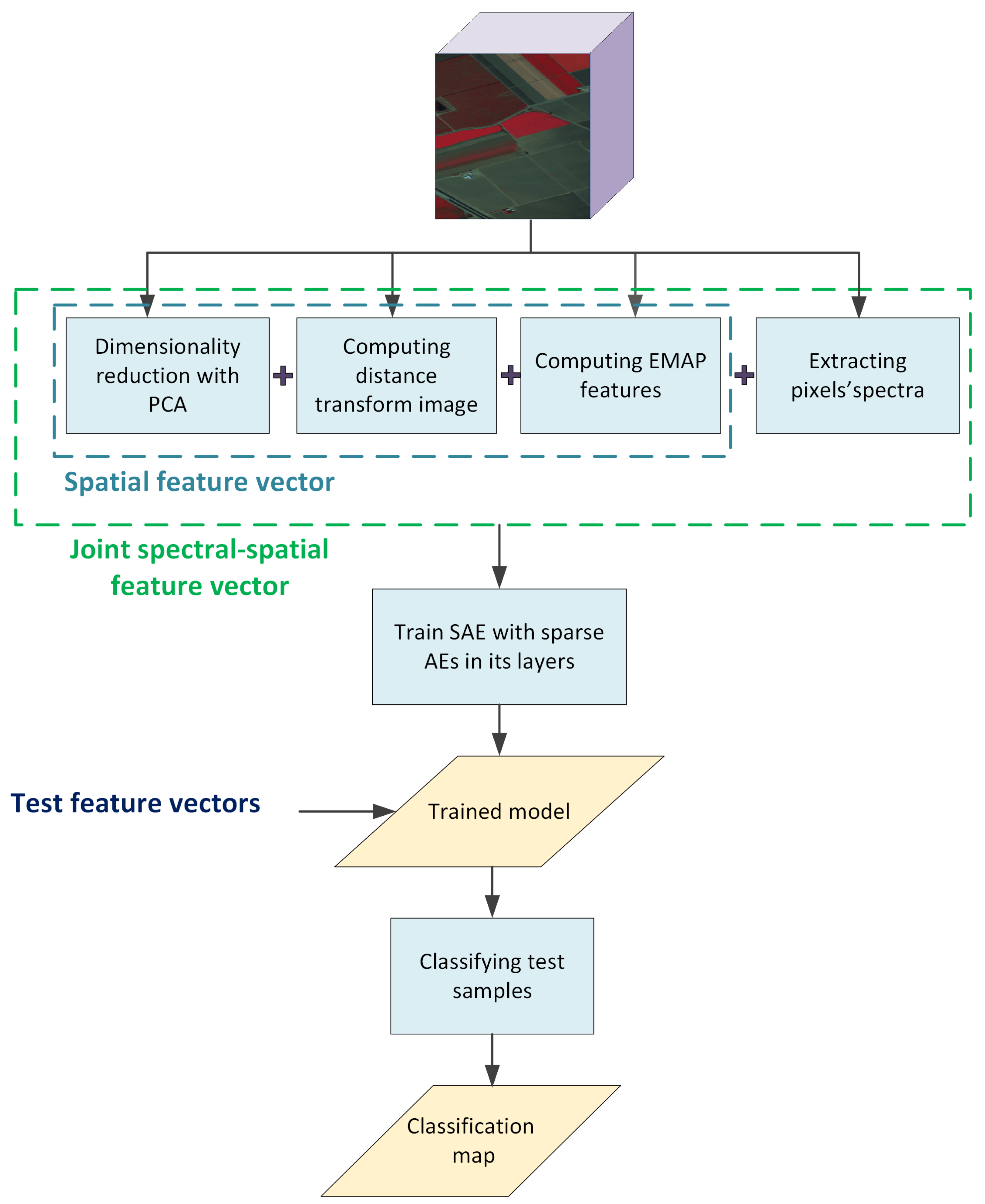
In this paper, we proposed a novel approach for spectral-spatial feature extraction. We weight pixels based on their difference to significant edges in the image based on the assumption that pixels well-separated from the boundaries of geometric regions are more likely to be representative of the whole region than pixels towards the edge. We first calculate the gradient image of the input HSI. We then use the results from a distance transform for each pixel with respect to the dominant edges to augment the pixel’s spatial feature vector. To the best of our knowledge, this is the first time distance transform values are used in this way to add weights to a target pixel surrounding neighbors. Next, we augment the spatial feature vector with EMAP features in order to integrate further geometric information. Finally, the joint spectral-spatial feature vectors provide input to a two-layer stacked autoencoder including a sparse AE in each layer. The workflow diagram of our proposed HSI classification method is shown in Figure 1. We performed extensive experiments on three hyperspectral datasets and results show that our proposed method outperforms the other methods examined in this study.
The rest of this paper is organized as follows: In Section 2, a brief description of the algorithms including in our proposed method is presented. Section 3 presents our proposed feature extraction and classification framework. Experimental results and comparison to other methods are presented in Section 4 and Section 5. Finally, Section 6 concludes this paper.
2. Background
In this study, we used SAE with sparse AEs in its layers as the deep learning framework. So, in Section 2.1–Section 2.3, we describe the structure of these machine learning models and how they are used to extract features. To extract geometrical attributes from the input HSI and build our proposed feature vector, we utilized EMAP features as well. EAP is an extended attribute profile obtained using only one attribute (e.g., area) filter. Since we are interested in extracting different information from the image, we used extended multi attribute profiles which applies multiple attribute filters on each principal component image extracted from the input HSI. In Section 2.4, we provide a brief description of the EMAP features.
2.1. Autoencoder
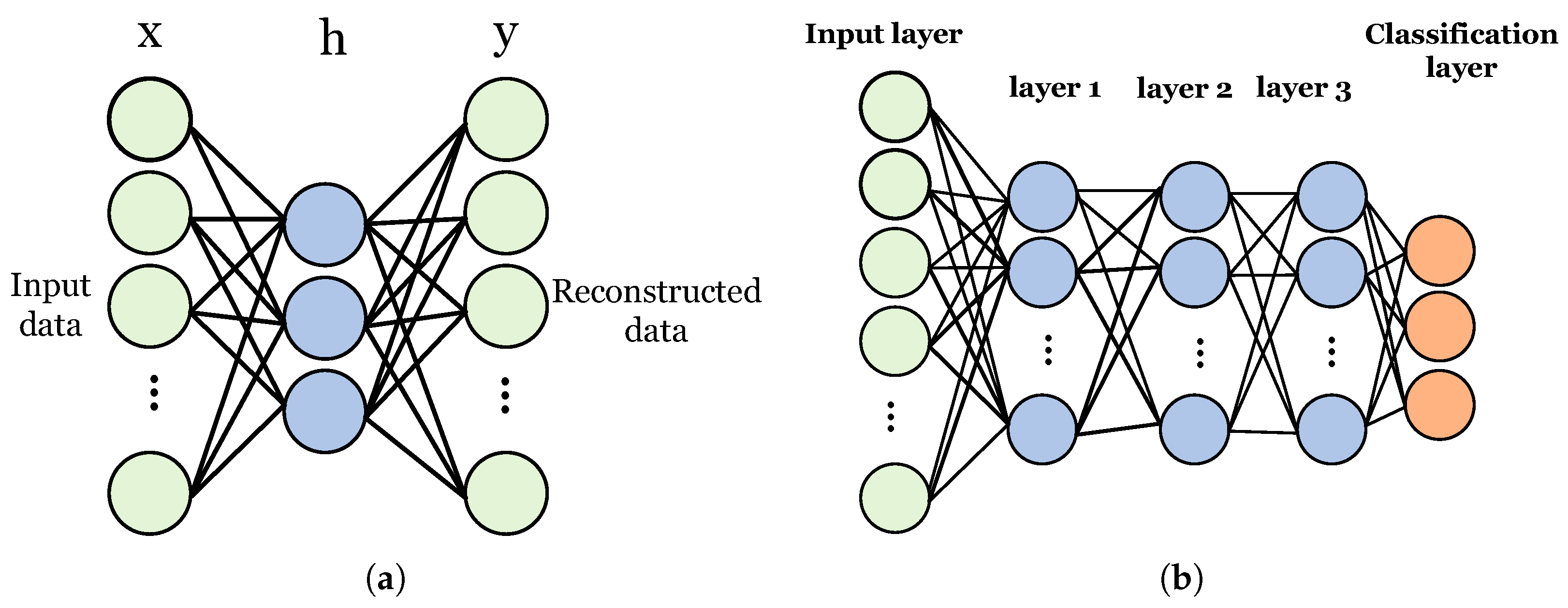
An autoencoder is a three-layer neural network with the goal of replicating its input into its output. These layers include input layer x, hidden layer h, and output layer y as shown in Figure 2a. Training an AE can be thought of as a two steps process: encoding and decoding. In the first step, input data is encoded to a new feature space and in the second part, input data is tried to be reconstructed using the extracted features during the encoding phase. The encoding and decoding processes can be formulated as Equations (1) and (2), respectively:
where and are the ith input and its corresponding hidden feature vector. represents the reconstructed version of . Also, f and g are the encoding and decoding functions. In practice, AEs are designed such that they cannot reproduce their input perfectly rather capable of delivering an approximation of the input. Since such a model is required to only copy important aspects of the data, it most likely represents favorable features of the input [22]. The goal of training an AE is to minimize the reconstruction error for all training samples through an optimization process which can be formulated as Equation (3):
where stands for the loss function. M and are the total number of training examples and the best set of parameters found during the optimization process, respectively.
2.2. Sparse Autoencoder
A sparse AE is a model whose training loss function involves a sparsity regularization term. This regularization term imposes the sparsity constraint on the output of the AE’s hidden layer and is a function of the mean of the output value of the hidden layer’s neurons [23]. This mean value can be represented as Equation (4):
where and are the vector of weights and the bias value of the jth neuron, respectively. A neuron is activated if its activation value is high enough. Having a low value for means that neuron j tends to be selective and respond only to that subset of the training data that includes specific features. Adding a term to the loss function that measures the difference between the and the desired neuron’s output value, called sparsity regularization, makes each neuron master learning features belonging to only a small portion of training samples. Kullback-Leibler divergence [24] can be considered as such sparsity regularization term:
where N and are the number of neurons in the hidden layer and the desired value for the average activation of each neuron, respectively. One drawback of having such a sparsity regularization term in the cost function is that during the training process, high values may be assigned to the weights of the network in order to maximize . To prevent this case to happen, a weight regularization term should be added to the AE’s cost function as shown in Equation (6):
where is the norm of the AE’s weight matrix. Finally, the cost function of the sparse AE can be expressed as Equation (7):
where and are the weight regularization and sparsity regularization coefficients, respectively.
2.3. Stacked Autoencoder
An SAE is composed of layers of AEs such that the hidden layer of AE in layer l becomes the input layer of the AE in layer as shown in Figure 2b. Training process of an SAE includes two steps: pre-training and fine-tuning.
During the pre-training step, each AE is trained individually in an unsupervised manner. Having trained an AE, the output layer with its weights and biases are removed and the hidden layer’s parameters are saved to be used for the next step. Also, except for the first AE whose input is the original data, the input of other AEs is the hidden features extracted from the previous AE.
In the fine-tuning step, the pre-trained AEs are put one after another with a classification layer on top to provide the supervised training. The input data is given to the AE in the first layer and the SAE is trained top to bottom. It should be noted that the hidden layers’ weights and biases which have been obtained from the pre- training step are used as the initial values during the SAE’s fine-tuning process.
2.4. Extended Multi-Attribute Profiles
Morphological attribute profiles (APs) [25] represent structural information in an image. They are extracted by the sequential application of morphological attribute filters. An attribute can be considered as any measure which can be computed on the connected component areas in an image. Examples of such attributes are area, length of the diagonal of the box bounding the region, length of the perimeter, image moments, standard deviation, etc. [13]. When the input data is a hyperspectral image, APs can be computed on the k principal components (PCs) extracted from the HSI which leads to the definition of the extended attribute profiles (EAP):
Since in practice, extracting different attributes from the image is desired, the concept of APs is expanded to EMAPs which applies multiple attribute filters on each PC image extracted from the input HSI:
where represents each of the n attributes used to compute the EMAP data structure. The prime sign indicates the exclusion of the original PC score image in forming the corresponding EAP to avoid the presence of each PC image multiple times in the final EMAP structure.
3. Methods
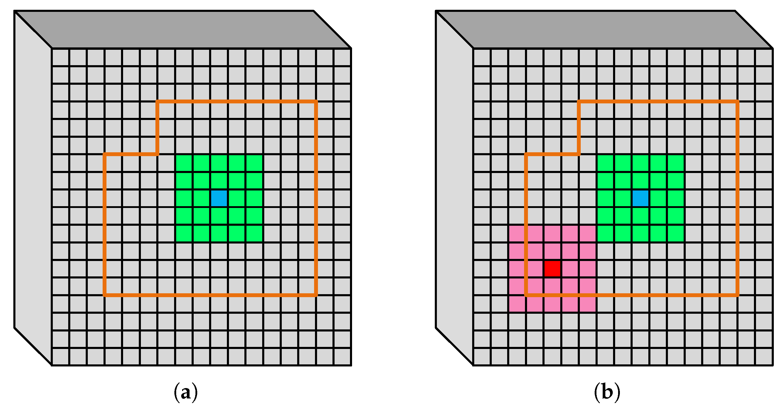
In pixel-wise classification, our goal is to group pixels according to their membership in a discrete set of classes (types). Spatial information can be used to enhance classification because it is likely that multiple pixels of the same class will be geometrically grouped together. Thus the classification of a particular pixel provides additional evidence towards the classification of its neighbours [15]. In our work, we have taken advantage of this tendency in a nuanced way. We predict that pixels away from the edges of a class should weigh more heavily in classification, because the likelihood that they will be similar to nearby pixels is assumed to be greater. A pixel at the edge of a region is likely to be near pixels of different classes, which means that its geometric location is less useful in classification. Consider the cases shown in Figure 3. In Figure 3a, the orange border enclosed a class of pixles of the same class. We have used the blue square to identify a pixel that is located well within the orange area. Green squares depict the neighborhood area around the blue pixel. Because the blue pixel is located well within the orange area far away from any boundary, our hypothesis is that this pixel and its neighbors should belong to the same class. Therefore, when we form the feature vector for the blue pixel, the spectral values of the green region will be included as features of the blue pixel. We treat pixels close to or on the border in the opposite way. Consider the red pixel and its pink neighbourhood depicted in Figure 3b. The red pixel is located close to a boundary, so its neighbours belong to multiple classes. In such cases as these, we would decrease the effect of the neighbors in the target pixel’s spatial feature by factoring in the (small) distance from the edge of the region. Our approach is to augment the feature vector with the value of each neighbor along with its distance transform value. This ensures that neighbours further from an edge are weighted more heavily, whereas neighbours nearer to an edge have their effect suppressed.
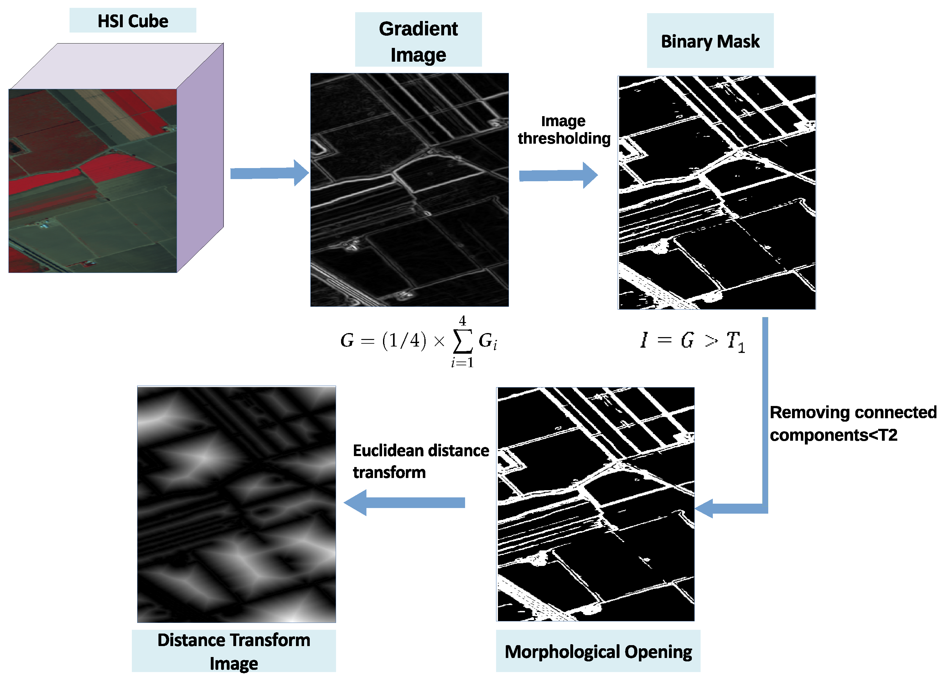
In order to find the distance transform image from an HSI cube (see Figure 4), we propose the following procedure: First, independently apply a Gaussian smoothing filter to each band of the HSI to suppress input noise. Next, we calculated the gradient image by employing the method described in [26].The aerial remote sensing scenes used in this study, consist of structures such as agricultural areas, roads and buildings representing edges at major directions as can be seen in Figure 5, Figure 6 and Figure 7. These edges represent borders of regions of different classes in each dataset. So, obtaining a gradient image which highlights these edges and so the borders of these regions is desired. Since HSI datasets are composed of many bands, we used the method described in [26] to obtain a one band gradient image from the entire dataset. This gradient image highlights the borders of the desired regions. This process is described as follows:
First, for each spectral band, we computed the image gradients at the four major directions 0°, 45°, 90°, and 135° using Sobel filters [27] according to Equation (10):
where is the image at band j, is the Sobel filter at one of the four specified directions, N is the total number of spectral bands, and is the gradient image of band j obtained from the ith Sobel filter. Also, * represents the convolution operation.
Next, to obtain the single image gradient for each direction, the corresponding gradients of all bands are added together:
where is the gradient image at direction i and N is the total number of spectral bands.
Finally, to compute the final gradient image of the whole HSI cube, the average of the four directional image gradients is computed:
where is the output gradient image of the input HSI.
Having calculated the gradient image, we apply a threshold to extract strong edges. Pixels with values greater than are labeled as foreground and the rest are labeled as background in the resulting binary mask. To remove small connected components in the thresholded image, first morphological opening is applied on the binary mask image and then connected components having fewer than pixels are removed from the image. In Section 4.2.3, we explain what values are chosen for these two hyperparameters. Finally, in order to find the distance of the pixels in the original image to the foreground (edge) pixels in the thresholded image, we used distance transform [28] with euclidean distance metric:
where and represent two pixels’ locations in the image. The distance transform yields a resulting image. The brightness of pixels in the transformed image indicates distance from the edge. Figure 4 illustrates how the process acts on an image from the Salinas HSI dataset.
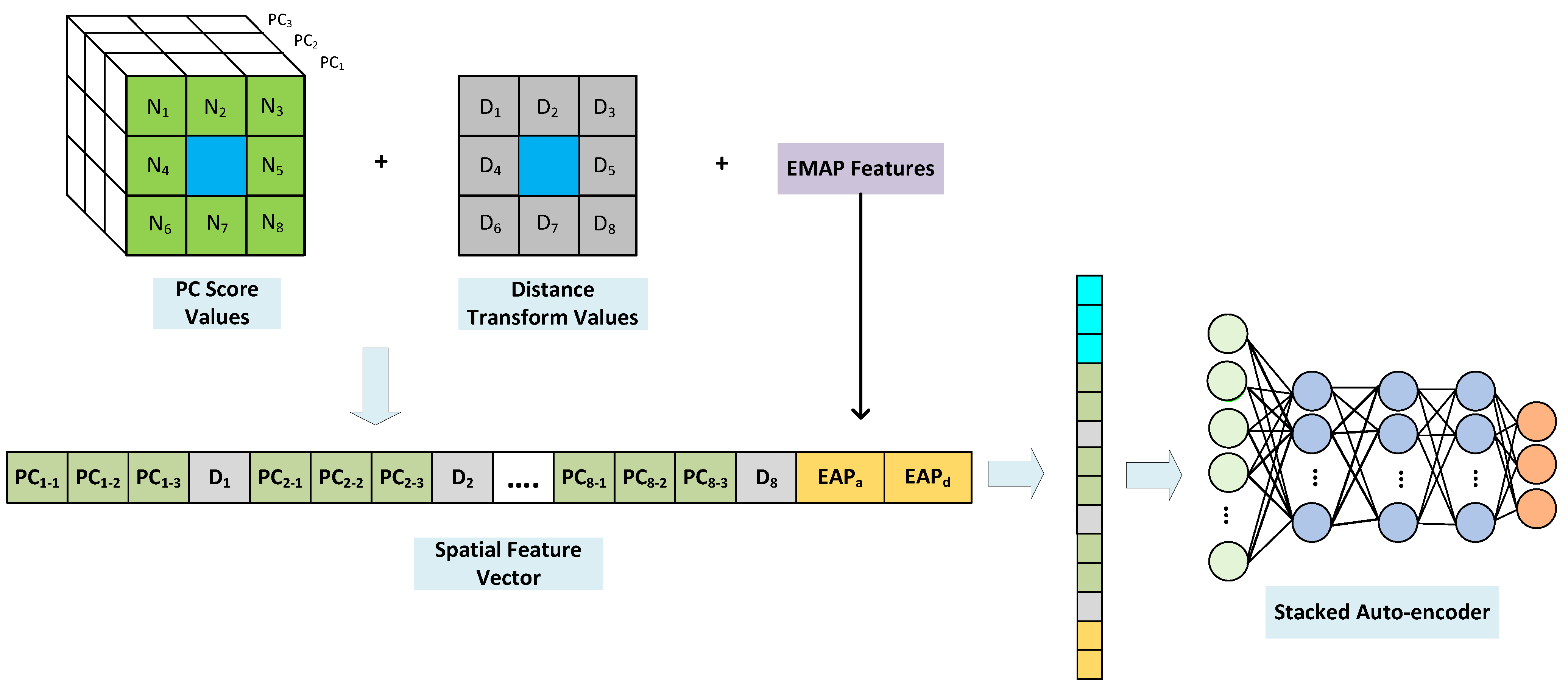
The spatial feature vector is then augmented with the distance transform values as is shown in Figure 8. To find the spatial features of the pixels in the HSI, similar to [14], we first reduced the dimension of the data along its spectral axis using the principal component analysis (PCA) method. Then, for each target pixel (blue square in Figure 8), a surrounding neighborhood area (green region) is considered. PCA searches for the most accurate data representation in a lower dimensional subspace composed of the uncorrelated linear combinations of the original variables called principal components. What PCA does is mapping the input data to the dimensions along which data vary the most. Since we are interested in reducing the dimensionality of the input data, we only keep the first few PCs which contain the most information of the original data. In Section 4.2.1, we talk about the number of preserved PCs in our experiments. To form the primary spatial feature vector, PC values of the neighbors and distance transform values from the corresponding distance transform image (Figure 4) are combined according to Equation (14):
where and represent the primary spatial feature vector associated with the target pixel and the ith pixel in the neighborhood region around this pixel, respectively. and represent a vector containing the PC score values and the distance transform value (scalar) associated with pixel , respectively. Also, indicates horizontal concatenation. Note that the distance transform values ( to ) can be placed either before or after each set of PC values for each neighbour of the target pixel. With this transformation, we ensure that the contribution of neighbour pixels in forming the target pixel’s spatial feature declines with proximity to edges of the region.
To compute the final proposed spatial feature vector and extract even more spatial information by adding geometric attributes to the primary spatial feature vector, similar to [16] we incorporated the EMAP features (see Section 2.4) as well. Finally, the pixel’s spectrum is added to the proposed spatial feature vector to form the input data to the stacked auto-encoder.
In Section 4, we test the effectiveness of our proposed method in classification of various remote sensing hyperspectral scenes. We performed two sets of experiments. In the first set of experiments (Proposed-P), we used only our primary proposed feature vector. In the second set of experiments (Proposed-F) we test our final feature vector that includes the EMAP features as well as the distance transform information.
In our Proposed-F feature vector to build the EMAP features for Salinas and University of Pavia datasets, we used area of the regions and the length of the diagonals of the regions’ bounding boxes as the regions attributes. For the Surrey dataset, area of the regions, length of the diagonals of the regions’ bounding boxes and standard deviation of the pixels in the regions are considered. For each attribute, an EAP is obtained from the first four PC images of the input HSI for all three datasets. For computing each AP, four different threshold values for filtering are used which are listed in Table 1.
4. Results
We have tested our method with applications to three hyperspectral datasets. The data sets are listed above (Section 4.1). The metrics used for the performance evaluation are class-specific accuracy, overall accuracy (OA), average accuracy (AA), Kappa coefficient, and the test time. In the experiments, we randomly picked 10% of the labeled samples for training and reserved the remaining 90% for testing. For each experiment we performed ten trials (with a different random selection each time). We have reported the mean value for each of the accuracy metrics along with the standard deviation. All experiments are performed using Matlab R2017a on a desktop with an Intel Core i7 3.7 GHz cpu and an NVIDIA GeForce GTX 1080 Ti gpu. Since all experiments have been performed on the same device, the test times are comparable.
4.1. Hyperspectral Datasets
In this study, we used three hyperspectral datasets. Salinas, University of Pavia (http://www.ehu.eus/ccwintco/index.php/Hyperspectral_Remote_Sensing_Scenes, accessed on 20 September 2019), and Surrey. Main characteristics of these datasets are listed in Table 2.
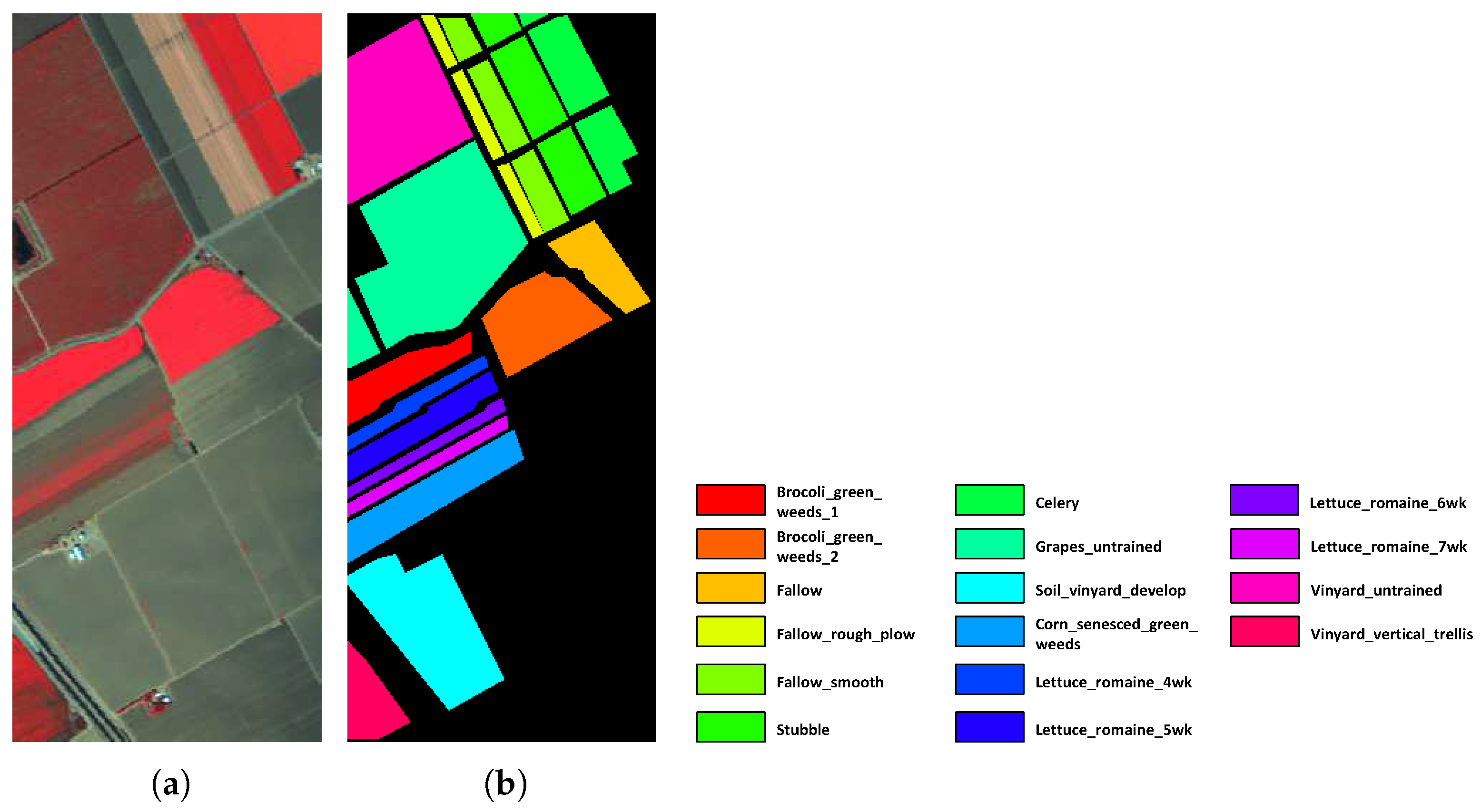
Salinas dataset was collected by the means of Airborne Visible/Infrared Imaging Spectrometer (AVIRIS) sensor in 1998 over Salinas Valley, California. Salinas hyperspectral dataset originally included 224 spectral bands. However, removal of 20 water absorption bands leaves only 204 bands of interest. This database contains an image of size 512 × 217 pixels in each band and has the high spatial resolution of 3.7 m. The ground truth of the Salinas scene covers 16 classes including vegetables, bare soil, and vineyard fields. Figure 5 shows the false color image of this dataset along with its pseudo color ground truth.
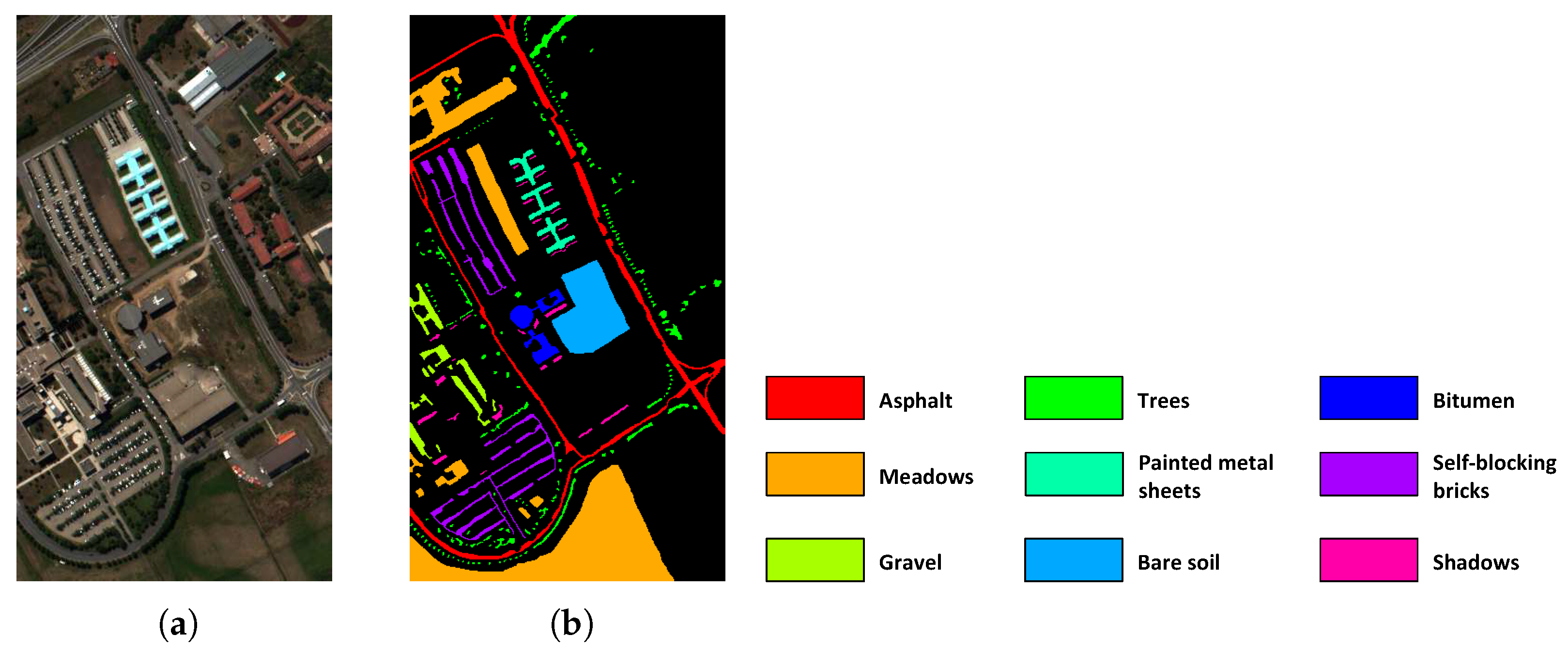
The University of Pavia database was gathered using a reflective optics system imaging spectrometer (ROSIS) sensor over the University of Pavia located in northern Italy. The University of Pavia dataset has 103 spectral bands in the wavelength range of 0.43–0.86 m. The spatial extent of each band is 610 × 340 pixels. The ground truth image contains 9 different classes. A true color image of this dataset and its corresponding pseudo color ground truth are shown in Figure 6.
The Surrey dataset is a novel data set collected by our team. In this work we have processed a small subset of a hyperspectral image captured by the airborne CASI-1500 sensor over the city of Surrey, BC, Canada in April 2013. This HSI includes 72 spectral bands in the range of 0.36 m to 1.05 m with the spectral resolution of 9.6 nm and the high spatial resolution of 1 m. The available ground truth includes 5 different classes. The false color and the pseudo color ground truth images are shown in Figure 7.
4.2. Parameter Tuning
Even though network’s parameters are tuned during the training step, there are hyperparameters in the model that need to be carefully set. These hyperparameters include the number of retained PCs during the dimensionality reduction step, n, size of the neighborhood region around each target pixel, s, number of the neurons in each layer of the network, and the required threshold parameters in the distance transform image acquisition process, and .
4.2.1. Number of Retained PCs and Size of the Neighborhood
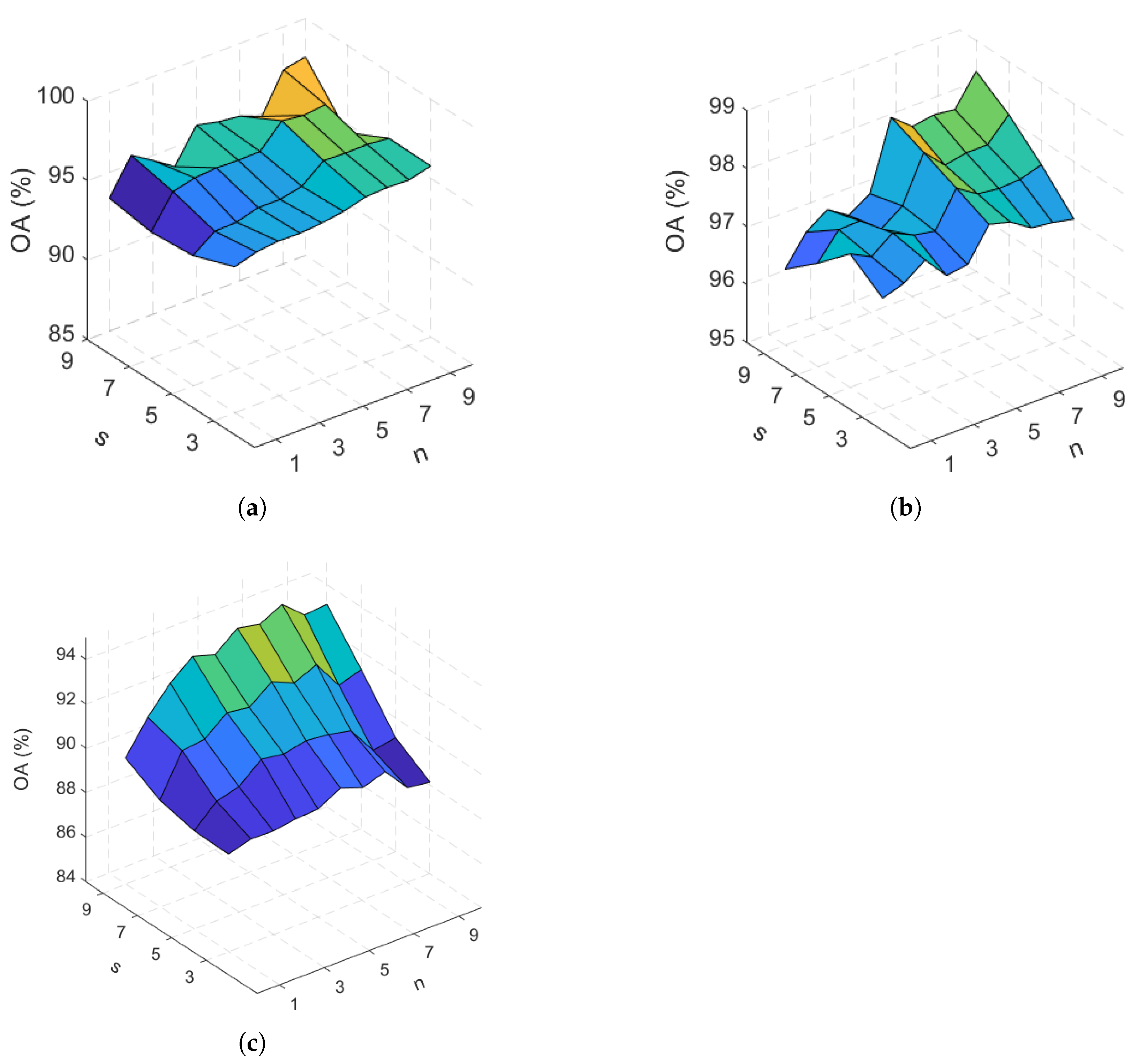
In this set of experiments, we used our primary proposed spatial feature vector and tried to find the best values for n and s hyperparameters. We considered keeping 1 to 10 PCs during the dimensionality reduction step. For the neighborhood size, we examined the following window sizes: , , , and . Distribution of the OA versus the aforementioned values for the two hyperparameters are depicted in Figure 9 for the three hyperspectral datasets.
As Figure 9a shows there is a general increase in the OA versus parameter n specially for and 7. Increasing the size of the neighborhood area has a positive effect on the OA as well. However, in the case of , for some values of n OA drops compared to some of its corresponding values for . Larger values for n and s result in increasing the size of the input vector to our deep network which consequently leads to having more trainable parameters. On the other hand, in general with larger n and s we achieve higher classification accuracies. Since larger neighborhood sizes has a more significant effect on increasing the accuracy than selecting more PCs, we chose the neighborhood size and set the n equal to 4 to decrease the computational cost. According to Figure 9b, OA generally increases with the increase of n. However, to have a trade off between the accuracy and the complexity of the feature vector, the value of 5 was chosen for this hyperparameter. Also, neighborhood window is chosen to be since it results in the best OA when n is set to be 5. For the Surrey dataset, we observed a general increase in the OA with the size of the neighborhood (Figure 9c). Increasing the value of parameter n results in a generally higher OA up to . To have an agreement between the accuracy and the size of the feature vector, similar to the case of University of Pavia, parameters s and n are chosen to be and 5, respectively. Table 3 summarizes all the selected values for parameters n and s for the three datasets.
4.2.2. Size of the Hidden Layers
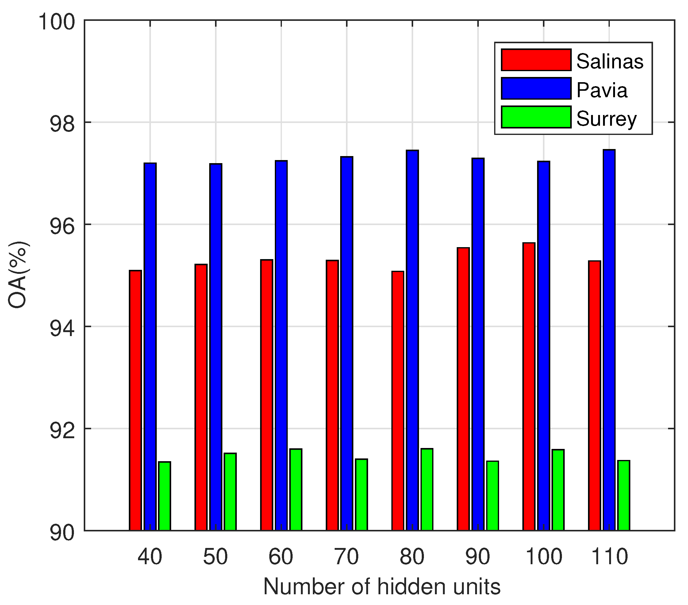
One of the hyperparameters that need to be set, is number of neurons in each layer. We tried eight values for this parameter for the three databases. Figure 10 shows the OA vs the size of the hidden layers for the three HSI databases. As can be seen from this figure, number of hidden units does not have much effect on the OA. So, in order to have an optimized number of trainable parameters in the network we chose the value of 60 for this hyperparameter for all three datasets.
4.2.3. Required threshold parameters
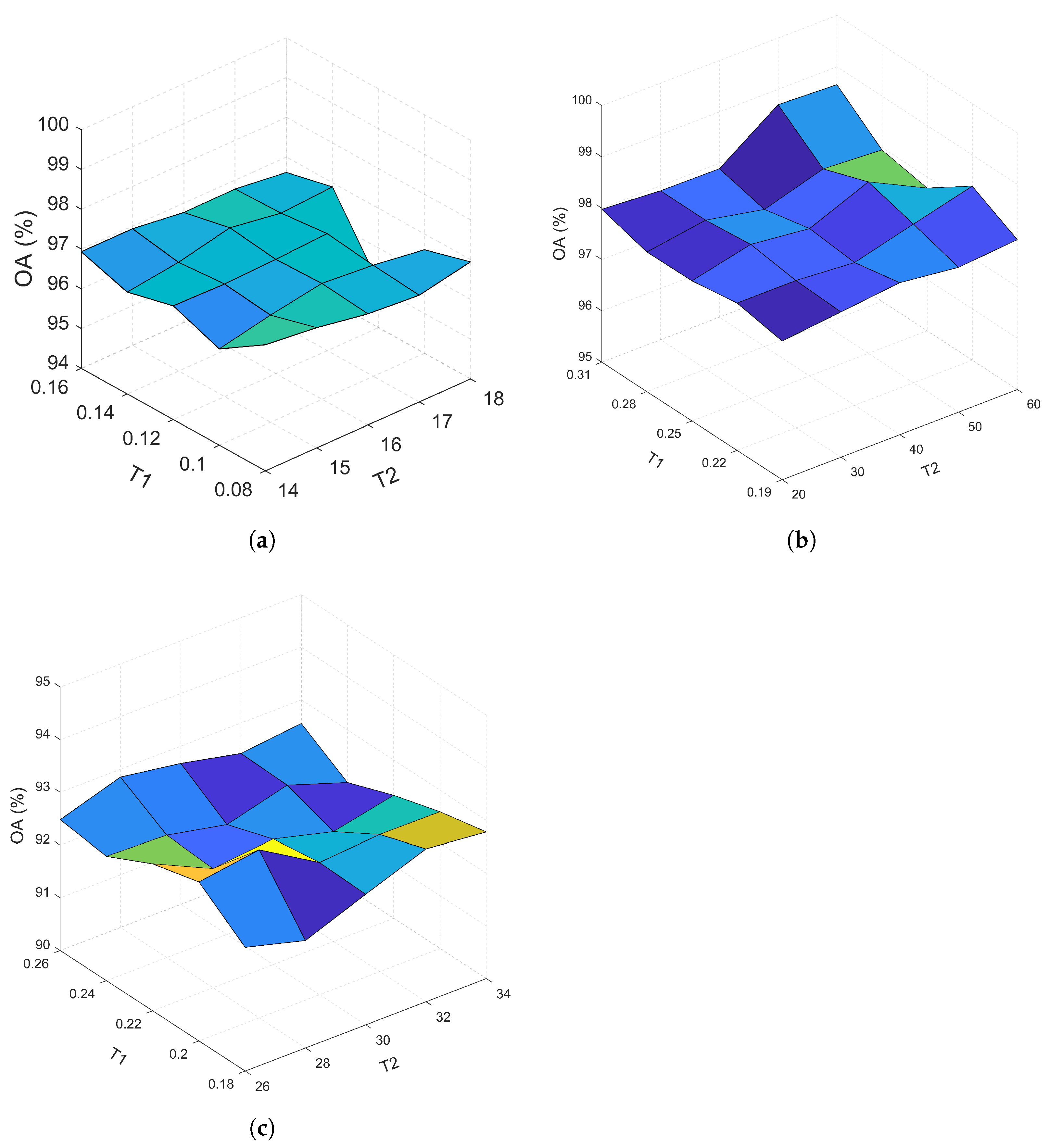
In our method, there are two thresholds in the process of obtaining the distance transform image of each dataset: A threshold above which pixels in the gradient image are considered strong edges , and a threshold for removing the connected components having fewer than P pixels in the binary mask image (see Figure 4) . We tried five different values for and for all three datasets in this study. Figure 11 shows the distribution of the OA versus the five values for these two parameters. For the Salinas dataset, and equal to 0.08 and 14 gave the highest OA. For the University of Pavia dataset, values of 0.31 and 50 for the and resulted in the highest OA. Also, for the Surrey dataset, and equal to 0.2 and 28 led to the best OA. Class specific accuracies, OA, AA, kappa coefficient, and the test time corresponding to these values are listed in the second last column of Table 4, Table 5 and Table 6. Corresponding classification maps are also shown in Figure 12, Figure 13 and Figure 14.
5. Discussion
To check the effectiveness of our proposed method, we compared it with some traditional and recent hyperspectral classification methods. These methods include linear SVM, Kernel SVM with radial basis function (RBF), extended multi-attribute profiles (EMAP), DAE [14], PPF-CNN [20], and EMAP-SAE [16]. We implemented both linear and kernel SVM using libsvm library [29].
We performed 10-fold cross validation to find the best values for the regularization parameter C and the width of the gaussian kernel gamma. For the Salinas database, value of for C in case of linear SVM and values of and 1 for C and gamma parameters of the gaussian SVM resulted in the best performance. For the University of Pavia dataset, C equal to 10 for the linear SVM and in case of the kernel SVM values of and 0.1 for C and gamma outperformed the other values. For the Surrey dataset, these values have been obtained as , , and 0.01, respectively. We used the kernel SVM classifier with the EMAP method and found the following values for the gaussian SVM’s parameters for the three datasets: Salinas: C = and gamma = 0.1, University of Pavia: C = and gamma = 0.001, and Surrey: C = and gamma = 0.01. With all other methods we used logistic regression (LR) classifier. Table 4, Table 5 and Table 6 compare the result of our proposed methods (using the Proposed-P and Proposed-F spatial feature vectors) with the other methods experimented in this study.
From these tables, we can draw the following conclusions. First, methods that combine spectral and spatial information achieve higher classification accuracies compared to the spectral-based approaches (L-SVM and K-SVM). Second, deep learning-based classifiers (i.e., DAE, PPF-CNN, EMAP-SAE, Proposed-P, and Proposed-F) outperform traditional HSI classification methods for almost all the accuracy metrics. In the DAE and EMAP-SAE methods, similar to our algorithm, joint spectral-spatial information and SAE is employed. However, they did not use the weighting strategy for neighboring pixels. So, by comparing the results of our Proposed-P feature vector with these two methods we can conclude that assigning different weights to the neighboring pixels improves the accuracy of the classification. Furthermore, this improvement shows the effectiveness of our proposed algorithm to compute such weights. The last column of these tables shows the results of our Proposed-F feature vector. The increase in the accuracy metrics compared to the results from our proposed primary feature vector shows the effectiveness of adding more geometric attributes on top of our proposed-P spatial feature vector. Therefore, as can be seen from these tables, adding the distance transform value to the feature vector and combining it with EMAP features improves accuracy metrics as well as the test time compared to the other methods. As an example, Table 7 summarizes the improvements made by our proposed methods compared to the EMAP-SAE [16] algorithm. For the Salinas dataset in terms of OA, adding only distance transform features (Proposed-P) improves the result by 2.27% compared to the EMAP-SAE method. For the University of Pavia and Surrey datasets, the corresponding increase in the OA is 0.57% and 2.07%, respectively. Furthermore, the kappa coefficient has been improved by 0.03, 0.01, and 0.03 for the three datasets, respectively. The increase in the AA compared to the EMAP-SAE method for the three datasets have been observed as 1.38 %, 0.65%, and 2.35%, respectively. The improvements made by our final feature vector (Proposed-F) are as follows: for the Salinas dataset the OA, AA and Kappa coefficient have been improved by 3.03%, 1.75%, and 0.04, respectively. The observed increase in these metrics for the University of Pavia dataset are 1.21%, 1.55%, and 0.02, respectively. Finally, we can see an improvement of 3.19%, 3.61%, and 0.04 for the Surrey dataset.
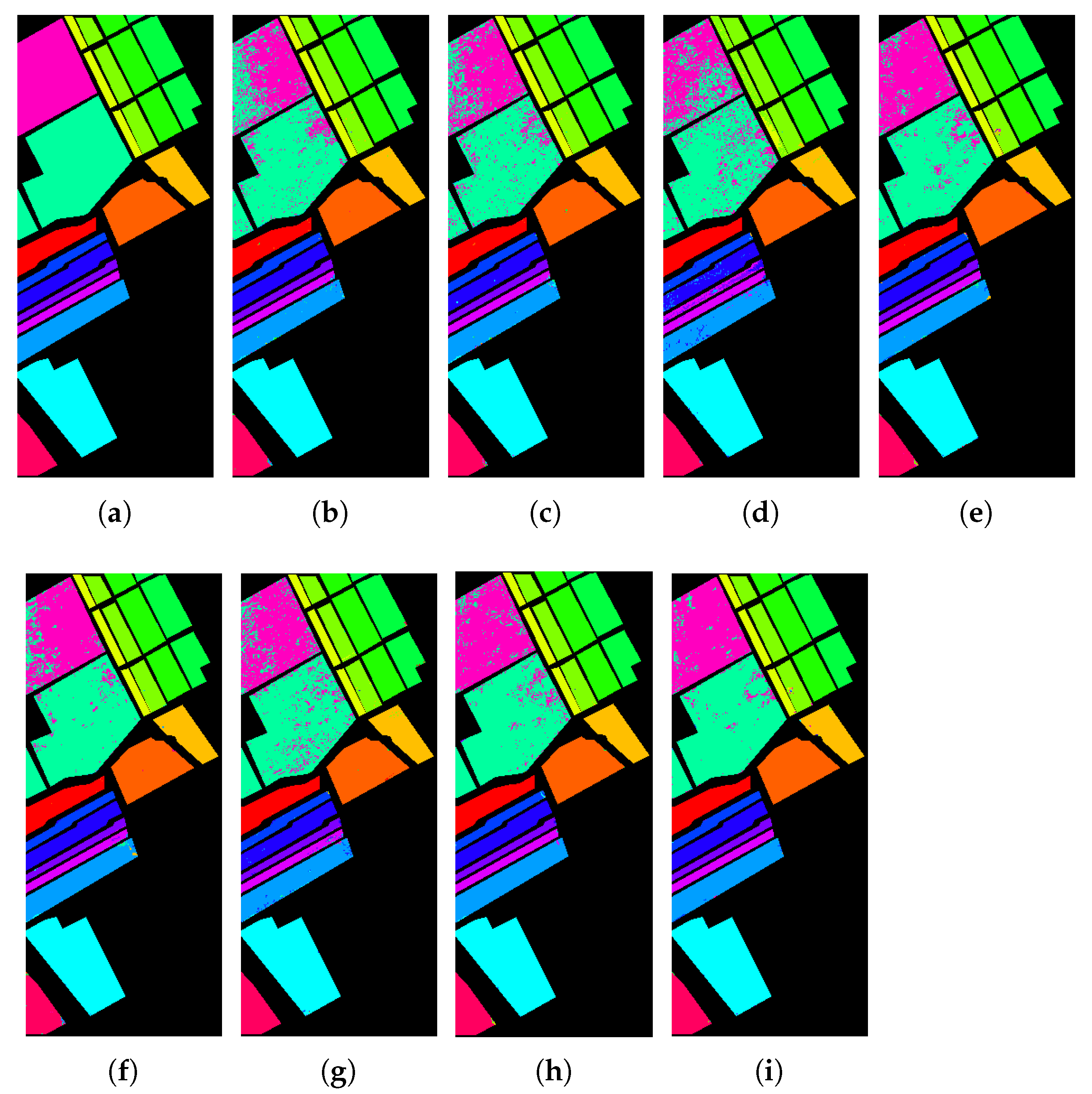
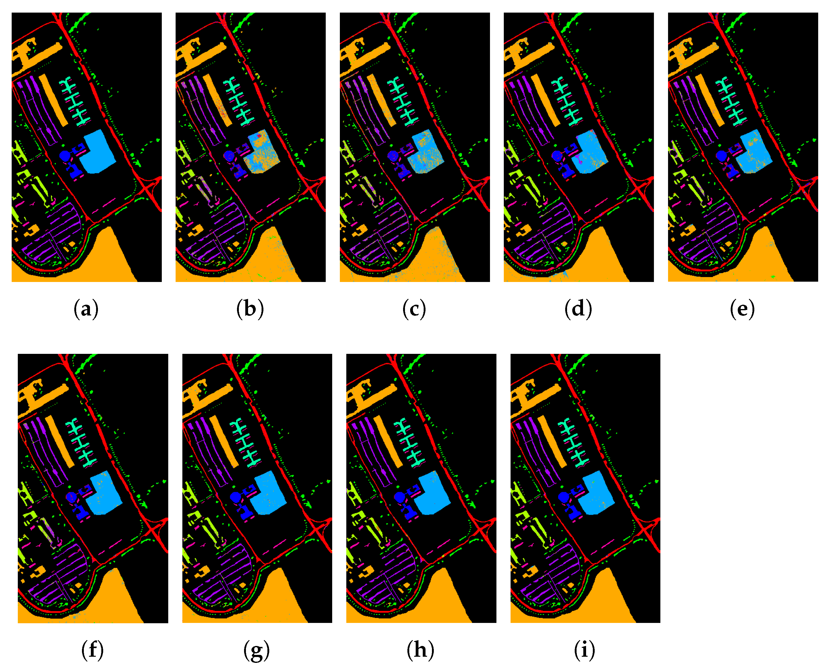
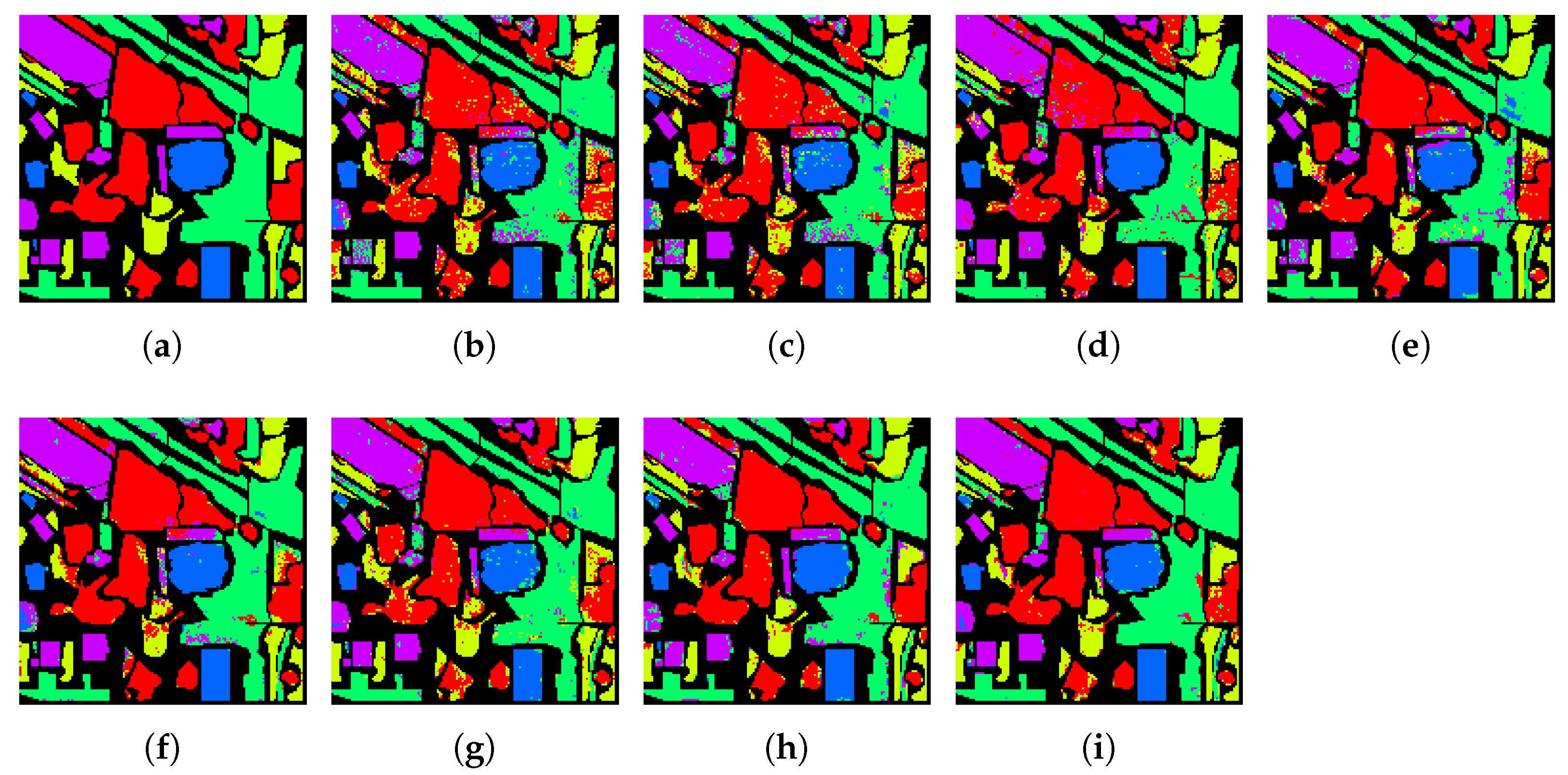
Figure 12, Figure 13 and Figure 14 show the classification maps obtained from our method and the other methods explored in this study. As can be seen from these figures, there are fewer misclassified pixels in our classification maps which is consistent with the results shown in Table 4, Table 5 and Table 6. For instance, according to Figure 12i (and also Table 4), our proposed final spatial feature vector especially improves the classification accuracies of classes 8 and 15 of the Salinas dataset. As Figure 13i shows, our proposed feature vector improves the classification accuracy of class 3 of the University of Pavia dataset significantly compared to other methods.
6. Conclusions
In this paper, we proposed a new method for the HSI classification task. In an HSI, pixels in a same region with a high probability belong to the same category. Therefore, the information of a target pixel’s neighbors may be used as the pixel’s spatial features. However, our conjecture in this work is that not all neighbours should be permitted to contribute to the same extent in forming the spatial feature vector for a target pixel. We hypothesize that pixels farthest from geometric boundaries are most likely to be located near neighbours of the same class, and as a result pixel distance from geometric edges should be used to weight the contribution of neighbouring pixels. Our proposed approach incorporates a new distance transform-based spatial feature vector which augments the spatial feature vector with the distance of pixels from the boundaries of geometric regions. The distance measure is obtained from a distance transform after some morphological processing of the input image. We use the stacked sparse autoencoder as the deep learning framework and train it based on a training data set with known classification. To find the best values for parameters of our method, we performed extensive experiments in the hyperparameter space. We also investigated the impact of geometric information by further augmenting the feature vector with EMAP features. We tested our method on three HSI datasets and based on our experimental results, we obtained the following findings. First, assigning different weights to the target pixel’s adjacent neighbors improved classification accuracies, in accordance with our hypothesis. We also saw an increase in classification accuracy with the inclusion of EMAP features in the spatial feature vector, which provides more support to the importance of spatial information in hyperspectral images. Regardless of the improvements made by our algorithm it has some limitations. First, since training and evaluation of our model should be done on each dataset separately, three different sets of the SAE’s weights and model’s hyperparameters are obtained. Second, since our model introduces several hyeprparameters that need to be tuned, a careful search in the hyperparameter space is needed.
Although the experimental results show that our method outperforms the other traditional and recent HSI classifiers experimented in this study, there is still work to be done in the future. For example, to test the generalization power of our algorithm, it should be tested on more remote sensing hyperspectral scenes acquired with various sensors. Training a unified model that can perform pixel-wise classification of these various remote sensing HSI scenes with a high accuracy is another future research goal. Moreover, with more computational power, we would need less time to explore more combinations of hyperparameter values in order to ensure our classification accuracy is maximized.
Author Contributions
Methodology, H.M. and K.M.; Software, H.M.;Writing—original draft, H.M.; Writing—review and editing, H.M., K.M. All the authors contributed significantly to the research. All authors have read and agreed to the published version of the manuscript.
Funding
This research was funded by NSERC Discovery Grant and CSA FAST 2019.
Institutional Review Board Statement
Not applicable.
Informed Consent Statement
Not applicable.
Data Availability Statement
Not applicable.
Acknowledgments
The authors would like to thank Jinfei Wang and Boyu Feng for providing us the Surrey dataset along with the ground truth image.
Conflicts of Interest
The authors declare no conflict of interest.
Nomenclature
| Average accuracy | |
| Auto encoder | |
| Attribute profile | |
| Airborne visible/infrared imaging spectrometer | |
| Convolutional neural network | |
| Deep belief network | |
| Extended attribute profile | |
| Extended multi-attribute profile | |
| Group-restricted Boltzmann machine | |
| Hyperspectral image | |
| K-nearest neighbor | |
| Principal component | |
| Principal component analysis | |
| Overall accuracy | |
| Restricted Boltzmann machine | |
| Rolling guidance filter | |
| Reflective optics system imaging spectrometer | |
| Stacked auto encoder | |
| Structural element | |
| Support vector machine |
References
- Dumke, I.; Nornes, S.M.; Purser, A.; Marcon, Y.; Ludvigsen, M.; Ellefmo, S.L.; Johnsen, G.; Søreide, F. First hyperspectral imaging survey of the deep seafloor: High-resolution mapping of manganese nodules. Remote Sens. Environ. 2018, 209, 19–30. [Google Scholar] [CrossRef]
- Jiang, M.; Cao, F.; Lu, Y. Extreme learning machine with enhanced composite feature for spectral-spatial hyperspectral image classification. IEEE Access 2018, 6, 22645–22654. [Google Scholar] [CrossRef]
- Li, F.; Zhang, P.; Huchuan, L. Unsupervised band selection of hyperspectral images via multi-dictionary sparse representation. IEEE Access 2018, 6, 71632–71643. [Google Scholar] [CrossRef]
- Guo, Y.; Cao, H.; Han, S.; Sun, Y.; Bai, Y. Spectral–spatial hyperspectralimage classification with k-nearest neighbor and guided filter. IEEE Access 2018, 6, 18582–18591. [Google Scholar] [CrossRef]
- Zhou, K.; Cheng, T.; Deng, X.; Yao, X.; Tian, Y.; Zhu, Y.; Cao, W. Assessment of spectral variation between rice canopy components using spectral feature analysis of near-ground hyperspectral imaging data. In Proceedings of the 2016 8th Workshop on Hyperspectral Image and Signal Processing: Evolution in Remote Sensing (WHISPERS), Los Angeles, CA, USA, 21–24 August 2016; pp. 1–4. [Google Scholar]
- Xie, A.; Sun, D.-W.; Xu, Z.; Zhu, Z. Rapid detection of frozen pork quality without thawing by vis–nir hyperspectral imaging technique. Talanta 2015, 139, 208–215. [Google Scholar] [CrossRef] [PubMed]
- zhang, C.; Guo, C.; Liu, F.; Kong, W.; He, Y.; Lou, B. Hyperspectral imaging analysis for ripeness evaluation of strawberry with support vector machine. J. Food Eng. 2016, 179, 11–18. [Google Scholar] [CrossRef]
- Munera, S.; Besada, C.; Aleixos, N.; Talens, P.; Salvador, A.; Sun, D.-W.; Cubero, S.; Blasco, A.J. Non-destructive assessment of the internal quality of intact persimmon using colour and vis/nir hyperspectral imaging. LWT Food Sci. Technol. 2017, 77, 241–248. [Google Scholar] [CrossRef] [Green Version]
- Di, W.; Zhang, L.; Zhang, D.; Pan, Q. Studies on hyperspectral face recognition in visible spectrum with feature band selection. IEEE Trans. Syst. Man Cybern. Part A Syst. Hum. 2010, 40, 1354–1361. [Google Scholar] [CrossRef] [Green Version]
- Ma, L.; Crawford, M.M.; Tian, J. Local manifold learning-based k-nearest-neighbor for hyperspectral image classification. IEEE Trans. Geosci. Remote Sens. 2010, 48, 4099–4109. [Google Scholar]
- Dalponte, M.; Ørka, H.O.; Gobakken, T.; Gianelle, D.; Næsset, E. Tree species classification in boreal forests with hyperspectral data. IEEE Trans. Geosci. Remote Sens. 2013, 51, 2632–2645. [Google Scholar] [CrossRef]
- Melgani, F.; Bruzzone, L. Classification of hyperspectral remote sensing images with support vector machines. IEEE Trans. Geosci. Remote Sens. 2004, 42, 1778–1790. [Google Scholar] [CrossRef] [Green Version]
- Mura, M.D.; Benediktsson, J.A.; Waske, B.; Bruzzone, L. Extended profiles with morphological attribute filters for the analysis of hyperspectral data. Int. J. Remote Sens. 2010, 31, 5975–5991. [Google Scholar] [CrossRef]
- Chen, Y.; Lin, Z.; Zhao, X.; Wang, G.; Gu, Y. Deep learning-based classification of hyperspectral data. IEEE J. Sel. Top. Appl. Earth Obs. Remote Sens. 2014, 7, 2094–2107. [Google Scholar] [CrossRef]
- Ma, X.; Wang, H.; Geng, J. Spectral-spatial classification of hyperspectral image based on deep auto-encoder. IEEE J. Sel. Top. Appl. Earth Obs. Remote Sens. 2016, 9, 4073–4085. [Google Scholar] [CrossRef]
- Teffahi, H.; Yao, H.; Chaib, S.; Belabid, N. A novel spectral-spatial classification technique for multispectral images using extended multi-attribute profiles and sparse autoencoder. Remote Sens. Lett. 2019, 10, 30–38. [Google Scholar] [CrossRef]
- Chen, Y.; Zhao, X.; Jia, X. Spectral-spatial classification of hyperspectral data based on deep belief network. IEEE J. Sel. Top. Appl. Earth Obs. Remote Sens. 2015, 8, 2381–2392. [Google Scholar] [CrossRef]
- Zhou, X.; Li, S.; Tang, F.; Qin, K.; Hu, S.; Liu, S. Deep learning with grouped features for spatial spectral classification of hyperspectral images. IEEE Geosci. Remote Sens. Lett. 2017, 14, 97–101. [Google Scholar] [CrossRef]
- Shu, L.; McIsaac, K.; Osinski, G.R. Hyperspectral image classification with stacking spectral patches and convolutional neural networks. IEEE Trans. Geosci. Remote Sens. 2018, 56, 5975–5984. [Google Scholar] [CrossRef]
- Li, W.; Wu, G.; Zhang, F.; Du, Q. Hyperspectral image classification using deep pixel-pair features. IEEE Trans. Geosci. Remote 2017, 55, 844–853. [Google Scholar] [CrossRef]
- Pan, B.; Shi, Z.; Xu, X. R-vcanet: A new deep-learning-based hyperspectral image classification method. IEEE J. Sel. Top. Appl. Earth Obs. Remote Sens. 2017, 10, 1975–1986. [Google Scholar] [CrossRef]
- Goodfellow, I.; Bengio, Y.; Courville, A. Deep Learning; MIT Press: Cambridge, MA, USA, 2016; Available online: http://www.deeplearningbook.org (accessed on 30 October 2019).
- Available online: https://www.mathworks.com/help/deeplearning/ref/trainautoencoder.html;jsessionid=4d6dead5aac0b2f61758450f8fc6 (accessed on 20 September 2019).
- Olshausen, B.A.; Field, D.J. Sparse coding with an overcomplete basis set: A strategy employed by v1? Vis. Res. 1997, 37, 3311–3325. [Google Scholar] [CrossRef] [Green Version]
- Mura, M.; Benediktsson, J.A.; Waske, B.; Bruzzone, L. Morphological attribute profiles for the analysis of very high resolution images. IEEE Trans. Geosci. Remote Sens. 2010, 48, 3747–3762. [Google Scholar] [CrossRef]
- Tarabalka, Y.; Fauvel, M.; Chanussot, J.; Benediktsson, J.A. Svm- and mrf-based method for accurate classification of hyperspectral images. IEEE Geosci. Remote Sens. Lett. 2010, 7, 736–740. [Google Scholar] [CrossRef] [Green Version]
- Gonzalez, R.C.; Woods, R.E. Digital Image Processing; Prentice Hall: Upper Saddle River, NJ, USA, 2008. [Google Scholar]
- Maurer, C.R.; Qi, R.; Raghavan, V. A linear time algorithm for computing exact euclidean distance transforms of binary images in arbitrary dimensions. IEEE Trans. Pattern Anal. Mach. 2003, 25, 265–270. [Google Scholar] [CrossRef]
- Available online: https://www.csie.ntu.edu.tw/%7Ecjlin/libsvm/ (accessed on 20 September 2019).
Figure 1.
The workflow diagram of our proposed method.

Figure 2.
Block diagram of (a) a sample autoencoder and (b) stacked autoencoder.

Figure 3.
Schematic of the justification of using the distance transform in the spatial feature vector. (a) Normal pixel case. (b) Border pixel case.
Figure 3.
Schematic of the justification of using the distance transform in the spatial feature vector. (a) Normal pixel case. (b) Border pixel case.

Figure 4.
Steps of our proposed process for obtaining the distance transform image from a hyperspectral dataset (here Salinas dataset is used as an input example).
Figure 4.
Steps of our proposed process for obtaining the distance transform image from a hyperspectral dataset (here Salinas dataset is used as an input example).

Figure 5.
Salinas dataset. (a) False color image. (b) Pseudo ground truth image.

Figure 6.
University of Pavia dataset. (a) True color image. (b) Pseudo ground truth image.

Figure 7.
Surrey dataset. (a) False color image. (b) Pseudo ground truth image.

Figure 8.
Block diagram of extracting the proposed spatial feature vector.

Figure 9.
OA obtained by our proposed primary spatial feature vector (Proposed-P) vs n and s for (a) Salinas, (b) University of Pavia, and (c) Surrey datasets.
Figure 9.
OA obtained by our proposed primary spatial feature vector (Proposed-P) vs n and s for (a) Salinas, (b) University of Pavia, and (c) Surrey datasets.

Figure 10.
OA versus number of hidden units in each layer for the three hyperspectral datasets.

Figure 11.
OA obtained by the Proposed-P feature vector vs parameters and for (a) Salinas, (b) University of Pavia, and (c) Surrey datasets.
Figure 11.
OA obtained by the Proposed-P feature vector vs parameters and for (a) Salinas, (b) University of Pavia, and (c) Surrey datasets.

Figure 12.
Salinas (a) ground truth, (b–i) classification maps resulting from different methods. (b) Linear SVM, (c) kernel SVM, (d) EMAP, (e) DAE, (f) PPF-CNN, (g) EMAP-SAE, (h) Proposed-P, and (i) Proposed-F.
Figure 12.
Salinas (a) ground truth, (b–i) classification maps resulting from different methods. (b) Linear SVM, (c) kernel SVM, (d) EMAP, (e) DAE, (f) PPF-CNN, (g) EMAP-SAE, (h) Proposed-P, and (i) Proposed-F.

Figure 13.
University of Pavia (a) ground truth, (b–i) classification maps resulting from different methods. (b) Linear SVM, (c) kernel SVM, (d) EMAP, (e) DAE, (f) PPF-CNN, (g) EMAP-SAE, (h) Proposed-P, and (i) Proposed-F.
Figure 13.
University of Pavia (a) ground truth, (b–i) classification maps resulting from different methods. (b) Linear SVM, (c) kernel SVM, (d) EMAP, (e) DAE, (f) PPF-CNN, (g) EMAP-SAE, (h) Proposed-P, and (i) Proposed-F.

Figure 14.
Surrey. (a) ground truth, (b–i) classification maps resulting from different methods. (b) Linear SVM, (c) kernel SVM, (d) EMAP, (e) DAE, (f) PPF-CNN, (g) EMAP-SAE, (h) Proposed-P, and (i) Proposed-F.
Figure 14.
Surrey. (a) ground truth, (b–i) classification maps resulting from different methods. (b) Linear SVM, (c) kernel SVM, (d) EMAP, (e) DAE, (f) PPF-CNN, (g) EMAP-SAE, (h) Proposed-P, and (i) Proposed-F.


Table 1.
Values of the thresholds used for obtaining each AP.
| Dataset | |||
|---|---|---|---|
| Salinas | [1000 2000 3000 5000] | [50 75 100 125] | - |
| Pavia University | [100 500 1000 5000] | [10 25 50 100] | - |
| Surrey | [1000 2000 3000 5000] | [50 75 100 125] | [20 30 40 50] |
Table 2.
Characteristics of the HSI datasets used in this study.
| Dataset | Image Size (Pixel) | Image Spatial Resolution (m) | Imaging Sensor | Nnumber of Spectral Bands | Wavelength Range (m) |
|---|---|---|---|---|---|
| Salinas | 512 × 217 | 3.7 | AVIRIS | 204 | 0.36–2.5 |
| Pavia University | 610 × 340 | 1.3 | ROSIS | 103 | 0.43–0.86 |
| Surrey | 150 × 150 | 1 | CASI-1500 | 72 | 0.36–1.05 |
Table 3.
Selected number of retained PCs and the neighborhood size for the three datasets.
| Dataset | n | s |
|---|---|---|
| Salinas | 4 | 7 × 7 |
| Pavia University | 5 | 7 × 7 |
| Surrey | 5 | 7 × 7 |
Table 4.
Class-specific accuracy(%), OA(%), AA(%), Kappa coefficient, and the test time related to the different methods for the Salinas dataset using 10% of the training data.
Table 4.
Class-specific accuracy(%), OA(%), AA(%), Kappa coefficient, and the test time related to the different methods for the Salinas dataset using 10% of the training data.
| No | Train | Test | L-SVM | K-SVM | EMAP | DAE | PPF-CNN | EMAP-SAE | Proposed-P | Proposed-F |
|---|---|---|---|---|---|---|---|---|---|---|
| 1 | 201 | 1808 | 99.39 | 99.60 | 100 | 99.61 | 99.17 | 99.87 | 100 | 99.90 |
| 2 | 373 | 3353 | 99.70 | 99.69 | 99.95 | 99.70 | 99.66 | 99.70 | 99.94 | 99.85 |
| 3 | 198 | 1778 | 99.58 | 99.63 | 99.84 | 98.49 | 98.38 | 99.35 | 100 | 99.30 |
| 4 | 139 | 1255 | 99.44 | 99.39 | 15.68 | 99.02 | 99.28 | 98.88 | 98.88 | 99.58 |
| 5 | 268 | 2410 | 98.87 | 98.93 | 98.40 | 98.01 | 98.56 | 98.76 | 99.46 | 98.68 |
| 6 | 396 | 3563 | 99.88 | 99.74 | 99.84 | 99.75 | 99.83 | 99.72 | 99.99 | 99.94 |
| 7 | 358 | 3221 | 99.75 | 99.58 | 99.86 | 99.24 | 99.81 | 99.47 | 99.86 | 99.63 |
| 8 | 1127 | 10,144 | 88.40 | 88.39 | 87.92 | 91.17 | 94.58 | 89.72 | 93.34 | 95.46 |
| 9 | 620 | 5583 | 99.81 | 99.80 | 99.84 | 99.74 | 99.82 | 99.73 | 99.91 | 99.83 |
| 10 | 328 | 2950 | 97.48 | 97.37 | 96.68 | 97.09 | 96.28 | 96.51 | 98.59 | 98.47 |
| 11 | 107 | 961 | 98.71 | 98.93 | 97.63 | 97.13 | 96.34 | 97.61 | 97.92 | 99.17 |
| 12 | 193 | 1734 | 99.79 | 99.92 | 94.51 | 99.92 | 99.81 | 99.44 | 99.85 | 100 |
| 13 | 92 | 824 | 99.11 | 99.61 | 29.70 | 99.42 | 98.54 | 97.63 | 99.27 | 99.94 |
| 14 | 107 | 963 | 97.32 | 97.79 | 95.12 | 98.68 | 96.36 | 95.53 | 98.18 | 99.47 |
| 15 | 727 | 6541 | 65.03 | 74.94 | 62.74 | 88.17 | 82.12 | 82.87 | 91.25 | 94.00 |
| 16 | 181 | 1626 | 98.73 | 98.71 | 99.83 | 97.79 | 97.79 | 99.25 | 99.75 | 98.86 |
| OA | 5415 | 48,714 | 92.42 ± 0.12 | 93.75 ± 0.13 | 88.45 ± 0.19 | 95.92 ± 0.22 | 95.75 ± 0.69 | 94.90 ± 0.12 | 97.17 ± 0.17 | 97.93 ± 0.15 |
| AA | 96.31 ± 0.11 | 97.00 ± 0.08 | 86.10 ± 0.12 | 97.68 ± 0.22 | 97.27 ± 0.46 | 97.13 ± 0.21 | 98.51 ± 0.11 | 98.88 ± 0.08 | ||
| Kappa | 0.91 ± 0.001 | 0.93 ± 0.001 | 0.87 ± 0.002 | 0.95 ± 0.002 | 0.95 ± 0.008 | 0.94 ± 0.001 | 0.97 ± 0.002 | 0.98 ± 0.002 | ||
| Test time (s) | 14.10 | 12.32 | 7.03 | 0.48 | 10.36 | 0.59 | 0.08 | 0.09 |
Table 5.
Class-specific accuracy(%), OA(%), AA(%), Kappa coefficient, and the test time related to the different methods for the University of Pavia dataset using 10% of the training data.
Table 5.
Class-specific accuracy(%), OA(%), AA(%), Kappa coefficient, and the test time related to the different methods for the University of Pavia dataset using 10% of the training data.
| No | Train | Test | L-SVM | K-SVM | EMAP | DAE | PPF-CNN | EMAP-SAE | Proposed-P | Proposed-F |
|---|---|---|---|---|---|---|---|---|---|---|
| 1 | 663 | 5968 | 85.04 | 89.17 | 90.08 | 94.45 | 98.82 | 98.20 | 97.29 | 99.29 |
| 2 | 1865 | 16,784 | 95.11 | 96.32 | 97.85 | 98.68 | 99.28 | 99.31 | 99.86 | 99.87 |
| 3 | 210 | 1889 | 68.05 | 71.97 | 93.75 | 86.26 | 82.30 | 94.13 | 96.87 | 99.09 |
| 4 | 306 | 2758 | 89.93 | 92.32 | 96.36 | 95.73 | 93.22 | 95.74 | 97.72 | 97.69 |
| 5 | 135 | 1210 | 99.62 | 99.47 | 99.31 | 99.64 | 99.73 | 99.02 | 99.83 | 99.61 |
| 6 | 503 | 4526 | 55.31 | 72.67 | 91.07 | 89.94 | 95.42 | 97.86 | 99.05 | 98.99 |
| 7 | 133 | 1197 | 72.79 | 75.23 | 89.66 | 85.03 | 87.05 | 98.43 | 97.31 | 99.72 |
| 8 | 368 | 3314 | 72.06 | 75.98 | 94.51 | 90.68 | 92.58 | 95.99 | 96.61 | 98.52 |
| 9 | 95 | 852 | 93.84 | 94.84 | 77.89 | 99.21 | 99.42 | 99.35 | 99.39 | 99.17 |
| OA | 4278 | 38,498 | 84.61 ± 0.23 | 88.61 ± 0.17 | 94.60 ± 0.07 | 95.11 ± 0.46 | 96.55 ± 0.32 | 98.13 ± 0.44 | 98.70 ± 0.10 | 99.34 ± 0.11 |
| AA | 81.31 ± 0.35 | 85.33 ± 0.45 | 92.28 ± 0.26 | 93.29 ± 0.62 | 94.20 ± 1.10 | 97.56 ± 0.46 | 98.21 ± 0.12 | 99.11 ± 0.18 | ||
| Kappa | 0.79 ± 0.003 | 0.85 ± 0.002 | 0.93 ± 0.001 | 0.93 ± 0.006 | 0.95 ± 0.004 | 0.97 ± 0.004 | 0.98 ± 0.001 | 0.99 ± 0.001 | ||
| Test time (s) | 8.74 | 6.51 | 4.07 | 0.25 | 7.03 | 0.35 | 0.06 | 0.07 |
Table 6.
Class-specific accuracy(%), OA(%), AA(%), Kappa coefficient, and the test time related to the different methods for the Surrey dataset using 10% of the training data.
Table 6.
Class-specific accuracy(%), OA(%), AA(%), Kappa coefficient, and the test time related to the different methods for the Surrey dataset using 10% of the training data.
| No | Train | Test | L-SVM | K-SVM | EMAP | DAE | PPF-CNN | EMAP-SAE | Proposed-P | Proposed-F |
|---|---|---|---|---|---|---|---|---|---|---|
| 1 | 412 | 3709 | 88.60 | 90.06 | 88.42 | 92.95 | 95.11 | 91.69 | 95.25 | 94.15 |
| 2 | 185 | 1662 | 68.40 | 73.11 | 83.92 | 83.69 | 75.92 | 82.66 | 90.55 | 88.58 |
| 3 | 438 | 3937 | 88.80 | 89.57 | 93.50 | 90.65 | 92.50 | 93.65 | 93.76 | 96.19 |
| 4 | 124 | 1117 | 91.54 | 91.20 | 98.38 | 90.68 | 96.72 | 92.45 | 94.28 | 96.49 |
| 5 | 215 | 1936 | 76.70 | 76.86 | 87.50 | 84.54 | 86.46 | 91.39 | 89.74 | 94.48 |
| OA | 1374 | 12,361 | 84.35 ± 0.43 | 85.66 ± 0.49 | 90.19 ± 0.46 | 89.45 ± 0.54 | 90.49 ± 0.47 | 91.12 ± 0.63 | 93.19 ± 0.27 | 94.31 ± 0.25 |
| AA | 82.81 ± 0.65 | 84.16 ± 0.81 | 90.34 ± 0.52 | 88.51 ± 0.66 | 89.34 ± 0.59 | 90.37 ± 0.75 | 92.72 ± 0.35 | 93.98 ± 0.24 | ||
| Kappa | 0.79 ± 0.006 | 0.81 ± 0.007 | 0.87 ± 0.006 | 0.86 ± 0.007 | 0.87 ± 0.006 | 0.88 ± 0.008 | 0.91 ± 0.003 | 0.92 ± 0.003 | ||
| Test time (s) | 2.31 | 1.02 | 1.5 | 0.18 | 6.91 | 0.24 | 0.05 | 0.06 |
Table 7.
The improvements made by our methods on the accuracy metrics compared to the EMAP-SAE [16] algorithm. The plus sign shows the improvement in the corresponding accuracy metric.
Table 7.
The improvements made by our methods on the accuracy metrics compared to the EMAP-SAE [16] algorithm. The plus sign shows the improvement in the corresponding accuracy metric.
| Proposed-P | Proposed-F | ||
|---|---|---|---|
| Salinas | OA | +2.27 | +3.03 |
| AA | +1.38 | +1.75 | |
| Kappa | +0.03 | +0.04 | |
| Pavia University | OA | +0.57 | +1.21 |
| AA | +0.65 | +1.55 | |
| Kappa | +0.01 | +0.02 | |
| Surrey | OA | +2.07 | +3.19 |
| AA | +2.35 | +3.61 | |
| Kappa | +0.03 | +0.04 | |
Publisher’s Note: MDPI stays neutral with regard to jurisdictional claims in published maps and institutional affiliations. |
© 2021 by the authors. Licensee MDPI, Basel, Switzerland. This article is an open access article distributed under the terms and conditions of the Creative Commons Attribution (CC BY) license (https://creativecommons.org/licenses/by/4.0/).
Share and Cite
MDPI and ACS Style
Madani, H.; McIsaac, K. Distance Transform-Based Spectral-Spatial Feature Vector for Hyperspectral Image Classification with Stacked Autoencoder. Remote Sens. 2021, 13, 1732. https://0-doi-org.brum.beds.ac.uk/10.3390/rs13091732
AMA Style
Madani H, McIsaac K. Distance Transform-Based Spectral-Spatial Feature Vector for Hyperspectral Image Classification with Stacked Autoencoder. Remote Sensing. 2021; 13(9):1732. https://0-doi-org.brum.beds.ac.uk/10.3390/rs13091732
Chicago/Turabian StyleMadani, Hadis, and Kenneth McIsaac. 2021. "Distance Transform-Based Spectral-Spatial Feature Vector for Hyperspectral Image Classification with Stacked Autoencoder" Remote Sensing 13, no. 9: 1732. https://0-doi-org.brum.beds.ac.uk/10.3390/rs13091732
Note that from the first issue of 2016, this journal uses article numbers instead of page numbers. See further details here.